Zero modes and divergence of entanglement entropy

Abstract

We investigate the cause of the divergence of the entanglement entropy for the free scalar fields in $(1+1)$ and $(D+1)$ dimensional space-times. In a canonically equivalent set of variables, we show explicitly that the divergence in the entanglement entropy of the continuum field in $(1+1)-$ dimensions is due to the accumulation of large number of near-zero frequency modes as opposed to the commonly held view of divergence having UV origin. The feature revealing the divergence in zero modes is related to the observation that the entropy is invariant under a hidden scaling transformation even when the Hamiltonian is not. We discuss the role of dispersion relations and the dimensionality of the space-time on the behavior of entanglement entropy.

I Introduction

Entanglement entropy, a popular measure to quantify quantum entanglement, has become a subject of intensive theoretical investigation, especially for systems with many degrees of freedom CardyQFT ; CardyCFT ; WilczekCFT and is being used to characterize properties of a wide spectrum of systems like quantum information processing 13 ; 3 , quantum phase transition sondhi ; sachdev and entropy of black holes Bombelli ; srednicki ; SolodukhinReview ; ShankiReview .

However, the entanglement entropy of free quantized fields is found to be divergent Bombelli ; WilczekGeometricEntropy and some form of regularization has to be used in order to extract useful information from it (also see SoloNestUVmodified ; PaddyZeroPointArea ; SoloNestShortDistReg in this context). Furthermore, in general, it is difficult to get an analytic handle on entanglement entropy except for a few special cases like $(1+1)$ dimensional CFTs CardyCFT .

In this work, with the aim to gain a better understanding of the divergence of entanglement entropy as well as to have better analytic control, we consider in detail the entanglement entropy of free scalar field regularized on a spatial lattice in $(1+1)$-dimensional space-time. With the insights gained in $(1+1)-$ dimensions, we extend the results to higher dimensions.

Specifically, we obtain analytical expression for the entanglement entropy by tracing over a single oscillator of the lattice regularized scalar field. The analytical expression provides two interesting features which, to our knowledge, have not been noted in the literature: (i) entanglement entropy is invariant under a scaling transformation even when the Hamiltonian is not, and (ii) the divergence in entanglement entropy in $(1+1)-$ dimensions in the continuum limit is due to the presence of a large number of near zero modes (and is not of UV origin as commonly believed). In the case of higher dimensions, accumulation of zero modes occur, however, the entropy remains finite (non-divergent).

The work is organized as follows. In the next section we start with the discretized version of free, massive scalar field in $(1+1)$ dimensions and define the covariance matrix for the corresponding Hamiltonian and show its relation to the entanglement entropy. In section (3), after performing a canonical transformation on the phase space of the scalar field theory, we show that the divergence of entanglement entropy in the continuum is due to the presence of near zero frequency modes. It is further shown that the entropy is divergent even when a single oscillator is traced over. Section (4) is devoted to regulating this divergence using a suitable infra-red cut-off. In section (5) we consider the effect of spatial dimensions on entanglement entropy of free fields. We conclude in section (6). We set $c=\hbar=1$.

II Entanglement entropy and covariance matrix in $(1+1)-$ dimensions

The system of interest is the $(1+1)$ dimensional massive, free scalar field theory described by the Lagrangian

$$L^{\rm(1D)}=\frac{1}{2}\int{\mathrm{d}}x\left(\dot{\phi}^{2}-(\nabla\phi)^{2}-m_{f}^{2}\phi^{2}\right),$$ (1)

where $m_{f}$ is the mass of the scalar field. The corresponding Hamiltonian is

$$H^{\rm(1D)}=\frac{1}{2}\int{\mathrm{d}}x\left(\pi^{2}+(\nabla\phi)^{2}+m_{f}^{2}\phi^{2}\right).$$ (2)

As mentioned earlier, the ground state entanglement entropy for such a system is divergent. In order to gain better understanding of the divergence, we place the system on a spatial lattice with lattice spacing $a$. Using the notation $\phi_{n}=\phi(x_{n})$ $(n\in\mathbb{I})$, where $x_{n}=an$ denotes the position of the lattice points, the discretized Hamiltonian is

$$H^{\rm(1D)}=\frac{1}{2}\sum_{n=0}^{N-1}\left(\frac{\pi_{n}^{2}}{a}+\frac{1}{a}(\phi_{n+1}-\phi_{n})^{2}+am_{f}^{2}\phi_{n}^{2}\right),$$ (3)

where $\pi_{n}=a\dot{\phi}_{n}$ is the canonically conjugate momentum of $\phi_{n}$. It is important to note that we have an infinite lattice in mind so that $N\rightarrow\infty$; the continuum limit corresponds to $a\rightarrow 0$. In the following we assume periodic boundary conditions $\phi_{0}=\phi_{N}$ (the final results are, however, independent of the specific choice of boundary conditions).

Our aim is to analytically calculate the entanglement entropy of the ground state wave-function of the above Hamiltonian obtained by tracing over first $m<N$ oscillators. This can be done by finding the ground state wave-function and then performing the partial trace. However, for greater generality, instead of taking this route, we calculate the entanglement entropy by finding the covariance matrix, which for the Hamiltonian (3) is the following $2N\times 2N$ matrix 3

$$\sigma = \frac{1}{2}\left[\begin{array}[]{cc}(aV)^{-1/2}&0\\ 0&(aV)^{1/2}\end{array}\right].$$ (6)

In the above equation $\omega_{k}$ are the normal mode frequencies

$$\omega_{k}^{2}=m_{f}^{2}+\frac{4}{a^{2}}\sin^{2}\left(\frac{\pi k}{N}\right),\,k=0,1,....,N-1$$ (7)

and $V$ is the potential matrix of the Hamiltonian (3). The matrix elements of the ‘position’ correlation $\Delta\phi=\frac{1}{2}(aV^{-\frac{1}{2}})$ and ‘momentum’ correlation $\Delta\pi=\frac{1}{2}(aV^{\frac{1}{2}})$ depend only on the separation $(i-j)$ between the $i$th and the $j$th oscillators.

The reduced state obtained after tracing over $m(<N)$ oscillators can be characterized from its covariance matrix $\sigma_{red}$ by picking appropriate elements from the total matrix. The entanglement entropy is given by 7

$$S_{m}(\rho_{red}) = \sum_{k=1}^{m}\left(\alpha_{k}+\frac{1}{2}\right)\log\left(\alpha_{k}+\frac{1}{2}\right)$$ (8)

$$-\left(\alpha_{k}-\frac{1}{2}\right)\log\left(\alpha_{k}-\frac{1}{2}\right).$$

where $\alpha_{k}$ are the symplectic eigen values of the reduced covariance matrix.

To have better analytic control in order to identify the scaling symmetry, we consider the simplest case of the single oscillator reduced system $(m=1)$, for which the covariance matrix is

$$\sigma_{red}=\frac{1}{2N}\left[\begin{array}[]{cc}\sum_{i}\frac{1}{a\omega_{i}}&0\\ 0&\sum_{j}a\,\omega_{j}\end{array}\right].$$ (9)

Here we would like to note a couple of things regarding the covariance matrix (9). The $1-1$ ($2-2$) element of the covariance matrix, often referred to in the literature as the ‘position’ (momentum) covariance 2012-Olivares-EPJ , is

$$\Delta\phi = \frac{1}{2N}\sum_{i=0}^{N-1}\frac{1}{\sqrt{a^{2}m_{f}^{2}+4\left(\sin^{2}\left(\displaystyle\frac{\pi i}{N}\right)\right)}}$$ (10)

$$\Delta\pi = \frac{1}{2N}\sum_{i=0}^{N-1}\sqrt{a^{2}m_{f}^{2}+4\left(\sin^{2}\left(\displaystyle\frac{\pi i}{N}\right)\right)}$$ (11)

In the continuum limit ($a\rightarrow 0$), the position covariance diverges while the momentum covariance is finite (non-zero value). Hence, the product $\Delta\phi\Delta\pi$, which is the determinant of the covariance matrix, diverges.

This determinant

$${Det(\sigma_{red})}=\frac{1}{4N^{2}}\sum_{i=0}^{N-1}\frac{1}{\sqrt{m_{f}^{2}+\frac{4}{a^{2}}\sin^{2}\left(\frac{\pi i}{N}\right)}}\sum_{j=0}^{N-1}\sqrt{m_{f}^{2}+\frac{4}{a^{2}}\sin^{2}\left(\frac{\pi j}{N}\right)}$$ (12)

is the eigenvalue $(\alpha_{1})^{2}$, from which the entropy can be calculated using (8).

The following points are worth noting regarding the above result: (i) the entropy is invariant under the scaling transformations

$$m_{f} \rightarrow \xi m_{f}$$

$$a \rightarrow \xi^{-1}a,$$ (13)

and (ii) in the continuum limit, $a\rightarrow 0$, $\omega^{2}_{k}\rightarrow\omega^{2}(k)=m_{f}^{2}+k^{2}$ and, with the summations going over to integrals, the entanglement entropy $S(\rho_{red})\rightarrow\infty$ since the numerator in (12) diverges for $k\rightarrow\infty$. This is the familiar UV-divergence of the entanglement entropy in the continuum.

In the next section, we show that the canonical transformation of the variables $(\phi,\pi)$ which accounts for the scaling symmetry will lead to a Hamiltonian that can be separated into a scale invariant and a scale dependent part. The entanglement entropy of the resultant Hamiltonian leads to a new way of identifying the cause of the divergence.

III Zero frequency modes and divergence of entanglement entropy

To take into account the scaling symmetry, we introduce the following canonical rescaling of the Hamiltonian (3)

$$\pi_{n}=\bar{\pi}_{n}(2+a^{2}m_{f}^{2})^{1/4},\quad\text{and}\quad\phi_{n}=\frac{\bar{\phi}_{n}}{(2+a^{2}m_{f}^{2})^{1/4}}.$$ (14)

In terms of these variables the Hamiltonian can be written as

$$H^{\rm(1D)}=\frac{E_{0}}{2}\sum_{n=0}^{N-1}\left(\bar{\pi}_{n}^{2}+\bar{\phi}_{n}^{2}-\beta\bar{\phi}_{n}\bar{\phi}_{n+1}\right).$$ (15)

Here we have defined

$$\beta = \frac{2}{2+a^{2}m_{f}^{2}},$$ (16)

$$E_{0} = \frac{(2+a^{2}m_{f}^{2})^{1/2}}{a}.$$ (17)

It is interesting to note that (i) under the scaling transformation (II), $E_{0}\rightarrow\xi E_{0}$ while $\beta$ is scale invariant. Thus, in writing the Hamiltonian (15), we have separated the scale invariant part of the Hamiltonian from the scale dependent part (which appears solely in the factor $E_{0}$). (ii) The canonical transformations (14) are well-defined for all values of $a$ (including the continuum limit whereby $\beta\to 1$ and $E_{0}\to\infty$). (The above canonical transformations have been discussed by Botero and Reznik 5 in a different context.)

Since the determinant of the covariance matrix and, hence, the entanglement entropy are invariant under the canonical transformations, we can express the determinant of the covariance matrix (12) in terms of $\beta$ by pulling out a factor of $4/a^{2}$ from both the numerator and the denominator leading to

$$\text{Det}(\sigma_{red}) = \frac{1}{4N^{2}}\sum_{i=0}^{N-1}\frac{1}{\sqrt{1-\beta+2\beta\sin^{2}\left(\frac{\pi i}{N}\right)}}$$ (18)

$$\sum_{j=0}^{N-1}\sqrt{1-\beta+2\beta\sin^{2}\left(\frac{\pi j}{N}\right)}.$$

This points to the fact that, for the purpose of evaluation of the entanglement entropy, instead of working with the full Hamiltonian (15), it is sufficient to work with the following ‘effective’ Hamiltonian

$$\bar{H}^{\rm(1D)}=\frac{1}{2}\sum_{n=0}^{N-1}\left(\bar{\pi}_{n}^{2}+\bar{\phi}_{n}^{2}-\beta\bar{\phi}_{n}\bar{\phi}_{n+1}\right),$$ (19)

from which we identify the following normal mode frequencies

$$\bar{\omega}_{i}=\sqrt{1-\beta+2\beta\sin^{2}\left(\frac{\pi i}{N}\right)}.$$ (20)

Note that $\bar{\omega}$ is related to the normal mode frequency $\omega$ defined in (7) by

$$\omega_{i}=\frac{2}{a}\bar{\omega}_{i}.$$ (21)

Thus, the resultant entanglement entropy depends only on the scale-invariant parameter $\beta$. As pointed out earlier, in the continuum limit $\beta$ is finite while $E_{0}$ diverges.

Eq. (18) gives insight into the real cause of the divergence. To understand this, let us first consider the case where $\beta\to 1$. For $i=0$ mode, the effective normal mode frequency is $\bar{\omega}_{0}=\sqrt{1-\beta}$. This implies that in Eq. (18) the discrete sum over $i$ would diverge because of the appearance of (at least) one term with zero in the denominator (the zero mode term). This shows that the divergence is due to the zero mode of $\bar{\omega}$. In fact, in this limit, large number of near-zero modes accumulate leading to the vanishing of the effective normal mode frequencies and hence divergence of the entanglement entropy.

Another (heuristic) way to understand how the innocuous canonical transformation (14) identifies the divergence of the entanglement entropy due to the near-zero modes is to look at the effective Hamiltonian (19). In the continuum limit, the last term on the right becomes

$$\beta\bar{\phi}_{n}\bar{\phi}_{n+1}\quad\rightarrow\quad\bar{\phi}_{n}^{2}$$

and this term cancels the second term in the Hamiltonian (19). Thus, in the continuum limit, there are large number of modes which effectively behave as free particles. In the context of quantum field theory, zero modes are excluded on the grounds that they are not normalizable and that they do not have particle interpretation. Although the zero modes have no physical effects, they carry 1989-Ford.Pathinayake-PRD an undetermined, non-zero energy $\langle{\bar{\pi}}^{2}\rangle/2$. This undetermined non-zero energy indicates the divergence of the entanglement entropy in $(1+1)$–dimensions.

IV Isolating the divergent contribution to entanglement entropy $\Delta S=S_{0}-S_{m}$

Having identified the divergence of the entanglement entropy in the continuum due to the presence of zero frequency modes, we still need to isolate the divergent term from the finite terms. We start by taking $N\rightarrow\infty$ limit in Eq. (18), and replace the summations by integrals (with $\pi i/N\rightarrow\lambda$)

$${Det(\sigma_{red})} = \frac{1}{\pi^{2}}\int_{0}^{\pi/2}\frac{d\lambda}{\sqrt{(1-\beta)+2\beta\sin^{2}(\lambda)}}$$ (22)

$$\times\int_{0}^{\pi/2}\sqrt{(1-\beta)+2\beta\sin^{2}(\lambda)}d\lambda.$$

In the continuum limit $\beta\rightarrow 1$, and as noted earlier, the first integral diverges. To isolate this divergence we introduce a cut-off function $f_{\delta}(\lambda)=e^{-\delta(\pi/2-\lambda)/\lambda}$ which has the desired property

$$f_{\delta}(\lambda)\rightarrow\begin{cases}\ 0&\text{when $\lambda\rightarrow 0$}\\ \ 1&\text{$\lambda\rightarrow\pi/2$}.\end{cases}$$

From the first integral in (22) it is clear that in the continuum ($\beta=1$) the divergent contribution comes only from the region $\lambda\approx 0$ where $\sin\lambda\approx\lambda$ and we get

$$\frac{1}{\pi}\left(\int_{0}^{\pi/2}\frac{1}{\lambda}e^{-\delta\frac{(\pi/2-\lambda)}{\lambda}}d\lambda\right)=e^{\delta}\int_{\delta}^{\infty}t^{-1}e^{-t}dt=\frac{1}{\pi}e^{\delta}\Gamma(0,\delta).$$ (23)

RHS of the above expression, in the limit when the cut-off parameter $\delta\rightarrow 0$, can be approximated by $(-\gamma-\log(\delta))$ where $\gamma\approx 0.57$ is the Euler-Mascheroni constant.

The remaining terms in the series expansion of $\sin\lambda$ in the first integral in (22) give a finite contribution of $\log(4/\pi)/\pi$ while the contribution from the second integral is $1/\pi$ (in evaluating these finite contributions we have put $\delta=0$).

Finally, using (8) for $m=1$, we find the entropy to be the sum of a finite contribution and a divergent contribution

$$S_{1} = \frac{1}{2}\log\left(\left(\frac{1}{\pi}\right)^{2}\left(\log(\frac{4}{\pi})-\gamma-\log(\delta)\right)\right)$$ (24)

$$\approx -\log(\pi)+\frac{1}{2}\log(\log(\frac{1}{\delta})).$$ (25)

It is interesting to note that the divergence in entropy is very slow going only as a double logarithm. Using the Boltzmann definition of entropy as logarithm of number of states, Eq. (24) gives

$$\Omega\sim\left(\frac{1}{\pi}\right)^{4}\left(\log\left(\frac{4}{\pi}\right)-\gamma-\log(\delta)\right)^{2}$$ (26)

The above expression explicitly shows that large number of near-zero modes ($\delta\to 0$) leads to the divergence of the entanglement entropy.

Until now, we have focused on the entanglement in $1:N-1$ partition as entanglement entropy can be evaluated analytically. It is straight forward to extend to a general partition $m:N-m$ using Eq. (8). However, for a general partition it is no longer possible to obtain analytic results and the determinant of the covariance matrix (18), for instance, has to be computed numerically.

Figure 1 shows the plot of entropy as a function of $m$ (the number of oscillators traced over) for different values of $\beta$ and it is seen to be an increasing function of $m$. Since entanglement entropy depends on the correlations across boundary 9 , one would expect that only oscillators near the boundary of the traced out region would contribute which would imply that the entropy should be a constant in $(1+1)$ dimensions even as more and more oscillators away from the boundary get traced out. In one dimensional chains, although this holds for weakly coupled chains as shown by Plenio et.al  6 , it breaks down in the strongly coupled systems srednicki and the entropy grows as $\log(m)$.

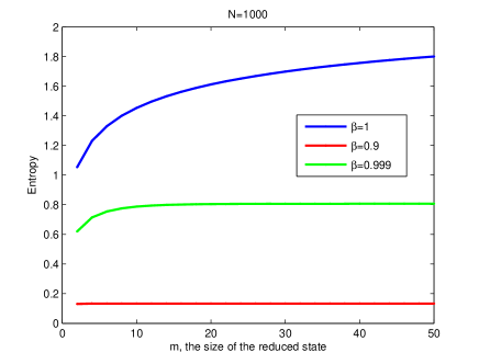
Figure 1: Entropy v/s the size of reduced state, with fixed boundaries. For $\beta=1$, the area law is violated

For the critical case of $\beta=1$, introducing the cut off function $f_{\delta}$ defined earlier, the entropy $(S)$ for $m$ oscillator reduced state gives a numerical fitting (ignoring the terms vanishing in $\delta\rightarrow 0$ limit)

$$S_{m}=C_{0}\log(m)+\frac{1}{2}\log\left(\log\left(\displaystyle\frac{1}{\delta}\right)\right)-\log(\pi),$$ (27)

where $C_{0}$ is a constant.

V Entanglement entropy in higher dimensions

To investigate the effects of dimensionality on the behavior of entanglement entropy, we first consider the scalar field in $(2+1)$ dimensions (discretized on a square lattice). The discretized version of the Hamiltonian for a scalar field in $(2+1)$ dimensions is

$$H^{\rm(2D)} = \sum_{i,j=1}^{N}\frac{P(i,j)^{2}}{2a^{2}}+\frac{1}{2}a^{2}m_{f}^{2}\eta(i,j)^{2}$$

$$+\frac{1}{2}\left[\eta(i+1,j)-\eta(i,j)\right]^{2}+\frac{1}{2}\left[\eta(i,j+1)-\eta(i,j)\right]^{2}.$$

Here $\eta(i,j)$ denotes the oscillator at position labeled by $(i,j)$ on the two dimensional lattice and $P(i,j)$ is the corresponding conjugate momentum. The Hamiltonian can be diagonalized by going to normal coordinates and the corresponding normal mode frequencies are (compare with Eq. (7) for $(1+1)$ dimensions)

$$\omega(i,j)=\sqrt{m_{f}^{2}+\frac{4}{a^{2}}\left(\sin^{2}\left(\displaystyle\frac{\pi i}{N}\right)+\sin^{2}\left(\displaystyle\frac{\pi j}{N}\right)\right)}$$ (29)

where $(i,j=0,1,\dots,N-1)$.

As in $(1+1)-$ dimensional case, the covariance matrix for the single oscillator reduced state is given by

$$\sigma_{red}=\frac{1}{2N^{2}}\left[\begin{array}[]{cc}\sum\limits_{k}\sum\limits_{l}\frac{1}{a^{2}\omega(k,l)}&0\\ 0&\sum\limits_{k}\sum\limits_{l}a^{2}\omega(k,l)\end{array}\right]\,.$$ (30)

The position and momentum covariance corresponding to the ground state of the Hamiltonian (V) are

$$\Delta\eta = \frac{1}{a}\frac{1}{2N^{2}}\sum_{i,j}\frac{1}{\sqrt{a^{2}m_{f}^{2}+4\left[\sin^{2}\left(\displaystyle\frac{\pi i}{N}\right)+\sin^{2}\left(\displaystyle\frac{\pi j}{N}\right)\right]}}~{}~{}~{}$$ (31)

$$\Delta P = \frac{a}{2N^{2}}\sum_{i,j}\sqrt{a^{2}m_{f}^{2}+4\left[\sin^{2}\left(\displaystyle\frac{\pi i}{N}\right)+\sin^{2}\left(\displaystyle\frac{\pi j}{N}\right)\right]}~{}~{}~{}~{}$$ (32)

Comparing the continuum limit of the above expressions with that of Eqs. (10,11) we notice that: (i) the position covariance diverges in both the cases, (ii) the momentum covariance vanishes in $(2+1)-$dimensions while it is a constant in $(1+1)-$dimensions. (iii) the determinant of the covariance matrix, remains finite in $(2+1)-$dimensions while it divergences in $(1+1)-$dimensions.

To explicitly see the finiteness of the determinant, let us replace the summations in (31, 32) with integrals (with $\theta\equiv\pi i/N$)

$$Det(\sigma_{red})=\frac{4}{(\pi)^{4}}\int_{0}^{\pi/2}\int_{0}^{\pi/2}\displaystyle\frac{d\theta_{1}d\theta_{2}}{\displaystyle\sqrt{\left(\sin^{2}\left(\theta_{1}\right)+\sin^{2}\left(\theta_{2}\right)\right)}}$$

$$\times\int_{0}^{\pi/2}\int_{0}^{\pi/2}\sqrt{\sin^{2}\left(\theta_{1}\right)+\sin^{2}\left(\theta_{2}\right)}d\theta_{1}d\theta_{2}.$$ (33)

Notice that, unlike $(1+1)$ dimensions, the result is finite as can easily be seen by replacing $\sin\theta\approx\theta$ (regions away from $\theta=0$ not contributing to the divergence).

The entanglement entropy is given by (8) and as in $(1+1)-$dimensional case, it is invariant under the scaling transformations:

$$m_{f} \rightarrow \xi m_{f}$$

$$a \rightarrow \xi^{-1}a,$$ (34)

and in the continuum limit, the entropy is divergent due to the UV modes.

Taking into account the scaling symmetry, introduce a canonical rescaling (similar to that in $(1+1)-$dimensions (14))

$$\bar{P}(i,j) = \displaystyle\frac{P(i,j)}{\left(a^{2}(4+a^{2}m_{f}^{2})\right)^{\frac{1}{4}}},$$

$$\bar{\eta}(i,j) = \eta(i,j)\left(a^{2}(4+a^{2}m_{f}^{2})\right)^{\frac{1}{4}}.$$ (35)

In terms of the transformed variables the Hamiltonian (V) becomes

$$H^{\rm(2D)} = \frac{E_{0}}{2}\sum_{j=1}^{N}\sum_{i=1}^{N}(\tilde{P}(i,j)^{2}+\tilde{\eta}(i,j)^{2}-\beta\tilde{\eta}(i,j)\tilde{\eta}(i+1,j)$$ (36)

$$-\beta\tilde{\eta}(i,j)\tilde{\eta}(i,j+1)),$$

where

$$E_{0}=\frac{\sqrt{4+a^{2}\,m_{f}^{2}}}{a};\qquad\beta=\frac{2}{(4+a^{2}\,m_{f}^{2})}.$$ (37)

It is important to highlight the differences between $(1+1)-$dimensions and higher dimensions: First, unlike Eqs. (II), canonical transformations (V) in $(2+1)-$ dimensions have an explicit $a$ dependence. This is due to the fact that the field and the canonically conjugate momentum $(\phi({\bf x},t),\pi({\bf x},t))$ have the dimensions $([L]^{-1/2},[L]^{1/2})$. In the case of $(1+1)-$ dimensions $\phi({x},t)$ ($\pi({x},t)$) are dimensionless. Hence, the strict $a=0$ is ill-defined in the case of $(2+1)-$ (or higher) dimensions,

Second, like in $(1+1)-$dimensions, the Hamiltonian (36) is separated into a scale invariant part and a scale dependent part. In the small $a$ limit, $\beta\to 1/2$. Third, the position and the momentum covariance corresponding to the rescaled Hamiltonian (36) are

$$\!\!\!\!\!\!\!\!\!\!\!\!\!\!\Delta\eta=\frac{1}{2N^{2}}\sum_{l,m}\frac{1}{\sqrt{1-2\beta+2\beta\sin^{2}\left(\frac{\pi l}{N}\right)+2\beta\sin^{2}\left(\frac{\pi m}{N}\right)}}$$ (38)

$$\!\!\!\!\!\!\!\!\!\!\!\!\!\!\Delta P=\frac{1}{2N^{2}}\sum_{l,m}\sqrt{1-2\beta+2\beta\sin^{2}\left[\frac{\pi l}{N}\right]+2\beta\sin^{2}\left[\frac{\pi m}{N}\right]}$$ (39)

are finite. This should be contrasted with the $(1+1)$ dimensional case where the canonical rescaling does not change the behavior of the position and momentum covariance.

Finally, like in $(1+1)$ dimensions, the entropy depends only on $\beta$ and, hence, it is sufficient to work with the following effective Hamiltonian

$$\bar{H}^{\rm(2D)} = \sum_{j=1}^{N}\sum_{i=1}^{N}(\bar{P}(i,j)^{2}+\bar{\eta}(i,j)^{2}-\beta\tilde{\eta}(i,j)\tilde{\eta}(i+1,j)$$ (40)

$$-\beta\tilde{\eta}(i,j)\tilde{\eta}(i,j+1)),$$

whose normal mode frequencies are

$$\bar{\omega}(i,j)=\sqrt{1-2\beta+2\beta\bigg{[}\sin^{2}\left(\frac{\pi i}{N}\right)+\sin^{2}\left(\frac{\pi j}{N}\right)\bigg{]}}.$$ (41)

Although the canonical transformations are not well-defined in $a\to 0$ limit, $\beta$ and normal mode frequencies are well-defined in this limit. The above calculation can be extended to any higher space dimensions. The only difference is that the critical value of $\beta=1/D$ where $D$ is the number of space dimensions.

Heuristically, as in the previous case, in $a\to 0$ limit, the last three terms in the RHS of the Hamiltonian (40) cancel giving rise to the free particle Hamiltonian. This shows that there is an accumulation of near-zero modes, however, unlike the previous case the contribution is non-divergent.

It is important to note that in both the cases [$(1+1)-$ and $(2+1)-$dimensional space-time], in the continuum limit, the entanglement entropy behaves differently. One possible explanation for this difference is the following: Entanglement entropy arises due to the correlations across the boundary 9 . In $(1+1)$ dimensions the boundary separating the two regions is the zero dimensional point and a single oscillator, occupying a point in space, is dense in the boundary (in the set-theoretic sense) leading to a divergent entropy. On the other hand, the boundary in $(2+1)$ dimensions is one dimensional and the single traced over oscillator, occupying a point is not dense in the 1-dimensional spatial boundary and, hence, the entropy is finite.

VI Conclusions

Entanglement entropy for free fields is divergent. In this work we revisited the question of the divergence in the light of zero modes. To obtain better analytic control we focused on the case where only a single oscillator (in the discretized version of free scalar field) was traced over. We found that the entanglement entropy has a scaling symmetry which the Hamiltonian does not possess. In terms of the canonically transformed variables, the Hamiltonian can be separated into a scale dependent and scale invariant part. We have shown that the origin of the divergence of the entanglement entropy in $(1+1)-$dimensions in the continuum limit is due the presence of accumulation of large number of (near-)zero frequency modes. In the context of quantum field theory, zero modes are excluded on the grounds that they are not normalizable and that they do not have particle interpretation. Although the zero modes have no physical effects, they carry 1989-Ford.Pathinayake-PRD an undetermined, non-zero energy $\langle{\bar{\pi}}^{2}\rangle/2$. Using an IR cutoff, we have shown that the undetermined non-zero energy leads to the divergence of the entanglement entropy in $(1+1)-$dimensions.

In higher dimensions, although, there is an accumulation of near-zero modes, their contribution to the entanglement entropy is non-divergent. One possible explanation for this difference between $(1+1)$ and higher dimensions is the following: Entanglement entropy arises due to the correlations across the boundary 9 . In $(1+1)$ dimensions the boundary separating the two regions is the zero dimensional point and a single oscillator, occupying a point in space, is dense in the boundary (in the set-theoretic sense) leading to a divergent entropy. On the other hand, the boundary in $(2+1)$ dimensions is one dimensional and the single traced over oscillator, occupying a point is not dense in the 1-dimensional spatial boundary and, hence, the entropy is finite.

References

- (1) P. Calabrese and J. L. Cardy, J. Stat. Mech. 0406, P06002 (2004) [hep-th/0405152].
- (2) P. Calabrese and J. Cardy, J. Phys. A 42, 504005 (2009) [arXiv:0905.4013].
- (3) C. Holzhey, F. Larsen and F. Wilczek, Nucl. Phys. B 424, 443 (1994) [hep-th/9403108].
- (4) R. Horodecki, P. Horodecki, M. Horodecki and K. Horodecki, Rev. Mod. Phys. 81, 865 (2009) [quant-ph/0702225].
- (5) J. Eisert, M. Cramer and M. B. Plenio, Rev. Mod. Phys. 82, 277 (2010) [arXiv:0808.3773].
- (6) S. L. Sondhi, S. M. Girvin, J. P. Carini and D. Shahar, Rev. Mod. Phys. 69, 315 (1997) [cond-mat/9609279].
- (7) S. Sachdev, Quantum Phase Transitions, Cambridge University Press, 2011, ISBN 9780521514682.
- (8) L. Bombelli, R. K. Koul, J. Lee, and R. D. Sorkin, Phys. Rev. D 34, 373 (1986).
- (9) M. Srednicki, Phys. Rev. Lett. 71, 666 (1993) [hep-th/9303048].
- (10) S. N. Solodukhin, Living Rev. Rel. 14, 8 (2011) [arXiv:1104.3712].
- (11) S. Das, S. Shankaranarayanan and S. Sur, Horizons in World Physics, edited by M. Everett and L. Pedroza, 268, 211 (Nova Science Publisheres, New York, 2009) [arXiv:0806.0402].
- (12) C. G. Callan, Jr. and F. Wilczek, Phys. Lett. B 333, 55 (1994) [hep-th/9401072].
- (13) D. Nesterov and S. N. Solodukhin, Nucl. Phys. B 842, 141 (2011) [arXiv:1007.1246].
- (14) T. Padmanabhan, Phys. Rev. D 82, 124025 (2010) [arXiv:1007.5066].
- (15) D. Nesterov and S. N. Solodukhin, JHEP 1009, 041 (2010) [arXiv:1008.0777].
- (16) S. L. Braunstein and P. van Loock, Rev. Mod. Phys. 77, 513 (2005).
- (17) S. Olivares, European Phys. J. Special Topics 203, 3 (2012).
- (18) A. Botero and B. Reznik, Phys. Rev. A 70, 052329 (2004) [quant-ph/0403233].
- (19) S. Das and S. Shankaranarayanan, Class. Quant. Grav. 24, 5299 (2007) [gr-qc/0703082].
- (20) M. B. Plenio, J. Eisert, J. Dreissig and M. Cramer, Phys. Rev. Lett. 94, 060503 (2005) [quant-ph/0405142].
- (21) L. H. Ford and C. Pathinayake, Phys. Rev. D 39, 3642 (1989).