An Efficient Quantum Jump Method for Coherent Energy Transfer Dynamics in Photosynthetic Systems under the Influence of Laser Fields

Abstract

We present a non-Markovian quantum jump approach for simulating coherent energy transfer dynamics in molecular systems in the presence of laser fields. By combining a coherent modified Redfield theory (CMRT) and a non-Markovian quantum jump (NMQJ) method, this new approach inherits the broad-range validity from the CMRT and highly efficient propagation from the NMQJ. To implement NMQJ propagation of CMRT, we show that the CMRT master equation can be casted into a generalized Lindblad form. Moreover, we extend the NMQJ approach to treat time-dependent Hamiltonian, enabling the description of excitonic systems under coherent laser fields. As a benchmark of the validity of this new method, we show that the CMRT-NMQJ method accurately describes the energy transfer dynamics in a prototypical photosynthetic complex. Finally, we apply this new approach to simulate the quantum dynamics of a dimer system coherently excited to coupled single-excitation states under the influence of laser fields, which allows us to investigate the interplay between the photoexcitation process and ultrafast energy transfer dynamics in the system. We demonstrate that laser-field parameters significantly affect coherence dynamics of photoexcitations in excitonic systems, which indicates that the photoexcitation process must be explicitly considered in order to properly describe photon-induced dynamics in photosynthetic systems. This work should provide a valuable tool for efficient simulations of coherent control of energy flow in photosynthetic systems and artificial optoelectronic materials.

1 Introduction

During the past decade, much progress has been achieved in both experimental and theoretical explorations of photosynthetic excitation energy transfer (EET), e.g., EET pathways determined by pump-probe as well as two-dimensional electronic spectroscopy (2DES) [1, 2, 3], coherent EET dynamics revealed by 2DES [4, 5, 6], and theoretical studies to elucidate mechanisms of EET [7, 8, 9, 10]. It is intriguing to consider the possibility of using laser pulse to coherently control energy flow in photosynthetic complexes. Notably, coherent light sources were adopted to control energy transfer pathways in LH2 [11]. The phases of the laser field can efficiently adjust the ratio of energy transfer between intra- and inter-molecule channels in the complex’s donor-acceptor system. In addition, theoretical control schemes were put forward to prepare specified initial states and probe the subsequent dynamics [12], and the optimal control theory has been adopted to optimize the effects of electromagnetic field’s polarization and structural and energetic disorder on localizing excitation energy at a certain chromophore within a Fenna-Matthews-Olson complex of green bacteria [13].

However, although the breakthroughs in experimental techniques have provided much insight into the coherent dynamics in small photosynthetic systems [14, 15], efficient theoretical methods that can describe quantum dynamics in realistic photosynthetic antenna are still lacking, because the typical size of an antenna ($>100$ chromophores) and the warm and wet environment make the accurate description of coherent EET in these systems a formidable task. Methods for simulating coherent EET dynamics in photosynthetic systems have been put forward (see [9] for a comprehensive review). For example, Förster theory directly provides EET rates, however it neglects quantum coherence effects that have been shown to be critical in photosynthetic systems [7]. In contrast, Redfield theory describes coherent EET dynamics, but it is valid only when the system-bath interactions are sufficiently weak [16, 17]. In order to bridge the gap between these two methods, recent advances in theoretical methods have focused on new approaches valid in the intermediate regime. For example, the small-polaron master equation approach [18, 19, 20, 21] should provide a reasonable description of the EET dynamics in the intermediate regime, and the hierarchical equation of motion (HEOM) actually yields a numerically exact means to calculate EET dynamics [22, 23, 24].

Nevertheless, it is still difficult to apply these theoretical methods to a realistic photosynthetic antenna, which often exhibits $>100$ chromophores and static disorder, due to the formidable computational resources required. Moreover, to understand the fundamentals of light-matter interactions in photosynthetic light harvesting and realize laser control of energy flow in photosynthetic systems, explicit treatment of photo-excitation processes would be necessary. Furthermore, it was suggested recently that the photoexcitation condition determined by the nature of the photon source could strongly affect the appearance of EET dynamics in photosynthetic complexes [25, 26, 27, 28, 29]. As a result, the interplay between the photoexcitation process and ultrafast EET dynamics may be highly nontrivial, and it would be important to explicitly consider system-field interactions in a theoretical description of light harvesting. Therefore, an accurate yet numerically efficient method for simulating quantum dynamics in photosynthetic systems in the presence of coherent laser fields is highly desirable.

In this work, we combine a coherent modified Redfield theory (CMRT) [30] and a non-Markovian quantum jump (NMQJ) method [31, 32, 33] to develop an efficient approach for coherent EET dynamics in photosynthetic systems under the influence of light-matter interactions. The modified-Redfield theory [34, 35] yields reliable population dynamics of excitonic systems and has been successfully applied to describe spectra and population dynamics in many photosynthetic complexes.[36, 37, 3] As a generalization of the modified-Redfield theory, the CMRT approach provides a complete description of quantum dynamics of the system’s density matrix. Furthermore, we adopt a quantum jump method to achieve efficient propagation of the CMRT equations of motion. Using quantum jumps or quantum trajectories to unravel a set of equations of motion for the density matrix into a stochastic Schrödinger equation has proven to be a powerful tool for the simulation of quantum dynamics in an open quantum system [38, 39, 40, 41, 31, 32]. In particular, Piilo et al. have developed a non-Markovian quantum jump (NMQJ) method that can be implemented for simulating non-Markovian dynamics in multilevel systems [31, 32]. To make use of the NMQJ method, which has been shown to be efficient for simulating quantum dynamics in EET [33, 42], we recast the CMRT equation into a generalized Lindblad form [43]. In addition, by transforming to a rotating frame, we extend CMRT to describe a time-dependent Hamiltonian, which is necessary to describe systems in the presence of laser fields. To examine the validity of the combined CMRT-NMQJ approach, we simulate the EET dynamics in the FMO complex. Moreover, we investigate a simple dimer system under the influence of laser pulses. We aim to shed light on how the photoexcitation process affects the coherence of EET dynamics in light harvesting.

This paper is organized as follows. In the next section, we briefly describe CMRT for EET in a dimer system with time-independent Hamiltonian. Then, we extend the CMRT to treat time-dependent case by including interactions with a laser pulse applied to the dimer. Furthermore, in order to make the CMRT suitable for time-propagation by the NMQJ method, we show that the CMRT quantum master equation can be rewritten in a generalized Lindblad form. In section 3, we detail the implementation of the NMQJ method to solve the CMRT master equation. To verify the applicability of the new method, in section 4, we apply it to simulate the EET dynamics in FMO and compare the results to those from numerically exact simulations. Furthermore, in section 5, we calculate the dynamics of site populations and entanglement in a dimer system after it has been excited by a laser pulse to investigate the interplay between laser excitation and ultrafast EET in the system. Finally, the main results of this work are summarized in section 6.

2 Coherent Modified Redfield Theory

For the sake of self-consistency, we briefly describe the CMRT method in this section. Note that the focus of this work is the combined CMRT-NMQJ approach. The details in the derivation and validity of the CMRT approach is outside of the scope of this paper and will be published elsewhere [30].

2.1 Time-Independent Hamiltonian

Before proceeding to the case with a time-dependent Hamiltonian, we briefly review the CMRT approach for a time-independent Hamiltonian. The CMRT approach is a generalization of the original modified Redfield theory [34, 35] to treat coherent evolution of the full density matrix of an excitonic system. For simplicity, we investigate the quantum dynamics in a dimer system (figure 1) described by the following excitonic Hamiltonian:

$$H_{S}^{(1)}=\sum_{n=1}^{2}E_{n}\left|n\right\rangle\left\langle n\right|+J\left(\left|1\right\rangle\left\langle 2\right|+\left|2\right\rangle\left\langle 1\right|\right)+E_{0}\left|G\right\rangle\left\langle G\right|,$$ (1)

where $\left|n\right\rangle$ is the product state of the excited state on the $n$th site and the ground state on the other site, i.e., $\left|1\right\rangle=\left|e\right\rangle_{1}\left|g\right\rangle_{2}$, $\left|2\right\rangle=\left|g\right\rangle_{1}\left|e\right\rangle_{2}$, $E_{n}$ is the corresponding site energy, $J$ is the electronic coupling between these two sites. Here, when there is no pulse applied to the system, the ground state $\left|G\right\rangle=\left|g\right\rangle_{1}\left|g\right\rangle_{2}$ with energy $E_{0}$ is decoupled to the single-excitation states $\left|n\right\rangle$. Note that although the Hamiltonian for a dimer system is considered in this work, the results can be straightforwardly generalized to treat multi-site systems, e.g. the FMO with seven sites as shown in section 4.

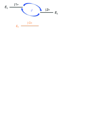
Figure 1: Energy diagram of a dimer for a time-independent case. The site energy for the single-excitation state $\left|n\right\rangle$ is $E_{n}$ and the energy of the ground state $\left|G\right\rangle$ is $E_{0}$. The electronic coupling $J$ between the single-excitation states is also considered.

Furthermore, the environment is modeled as a collection of harmonic oscillators described by the Hamiltonian

$$H_{B}=\sum_{n=1}^{2}\sum_{q}\left[\frac{p_{nq}^{2}}{2m_{q}}+\frac{1}{2}m_{q}\omega_{q}^{2}x_{nq}^{2}\right],$$ (2)

where $p_{nq}$ and $x_{nq}$ are respectively the momentum and position for $q$th harmonic oscillator on the $n$th site with mass $m_{q}$ and frequency $\omega_{q}$. Without loss of generality, we have assumed an independent bath for each site. Nevertheless, the CMRT can deal with a general system with correlated baths, whose effects on EET dynamics have been investigated in detail previously [44, 21, 45].

To describe exciton-bath interactions, we assume linear system-bath couplings described by

$$H_{SB} = \sum_{n=1}^{2}u_{n}\left|n\right\rangle\left\langle n\right|,$$ (3)

where the collective bath-dependent coupling is

$$u_{n} = \sum_{q}m_{q}\omega_{q}^{2}x_{nq}^{(0)}x_{nq},$$ (4)

where $x_{nq}^{(0)}$ denotes the displacement of the $q$th harmonic mode when the $n$th site is excited.For the electronic part, we diagonalize the system Hamiltonian in the exciton basis [7]

$$H_{S}^{(1)}=\sum_{k=0}^{2}\varepsilon_{k}^{\prime}\left|\varepsilon_{k}^{(1)}\right\rangle\left\langle\varepsilon_{k}^{(1)}\right|,$$ (5)

where each exciton basis state is a superposition of site-localized excitations

$$\left|\varepsilon_{k}^{(1)}\right\rangle=\sum_{n=0}^{2}C_{kn}^{(1)}\left|n\right\rangle,$$ (6)

with exciton energy $\varepsilon_{k}^{\prime}$. Since there is no interaction between the ground state and the single-excitation states, we have

$$\left|\varepsilon_{0}^{(1)}\right\rangle=\left|0\right\rangle=\left|G\right\rangle$$ (7)

with

$$\varepsilon_{0}^{\prime}=E_{0}.$$ (8)

In other words,

$$C_{0n}^{(1)}=\delta_{n0}.$$ (9)

Hereafter, for the sake of simplicity, we shall label $|G\rangle$ as $|0\rangle$.

Transforming $H_{SB}$ to the exciton basis, the system-bath interactions contain both diagonal and off-diagonal terms. Following the essence of the modified Redfield theory [34], we include the diagonal term of $H_{SB}$ into the zeroth-order Hamiltonian in the exciton basis to be treated nonperturbatively, and we only treat the off-diagonal term of $H_{SB}$ in the exciton basis as the perturbation. In the case, the unperturbed and perturbation Hamiltonians read respectively

$$H_{0}^{(1)} = \sum_{k=0}^{2}\left[\varepsilon_{k}^{\prime}+H_{B}+\sum_{n=1}^{2}u_{n}a_{kk}^{(1)}(n)\right]\left|\varepsilon_{k}^{(1)}\right\rangle\left\langle\varepsilon_{k}^{(1)}\right|,$$ (10)

$$V^{(1)} = \sum_{k=0}^{2}\sum_{k^{\prime}=0\left(\neq k^{\prime}\right)}^{2}\sum_{n=1}^{2}u_{n}a_{kk^{\prime}}^{(1)}(n)\left|\varepsilon_{k}^{(1)}\right\rangle\left\langle\varepsilon_{k^{\prime}}^{(1)}\right|,$$ (11)

where

$$a_{kk^{\prime}}^{(1)}(n) = C_{kn}^{(1)*}C_{k^{\prime}n}^{(1)}.$$ (12)

Notice that $a_{kk^{\prime}}^{(1)}(n)=0$ as long as $k=0$ or $k^{\prime}=0$ as a result of (9). We then apply the second-order cumulant expansion approach using $V^{(1)}$ as the perturbation followed by secular approximation to derive a quantum master equation for the reduced density matrix of the electronic system[34, 46, 30]:

$$\partial_{t}\rho=-\rmi\sum_{k,k^{\prime}}\left(\varepsilon_{k}^{(1)}-\varepsilon_{k^{\prime}}^{(1)}\right)\rho_{kk^{\prime}}\left|\varepsilon_{k}^{(1)}\right\rangle\left\langle\varepsilon_{k^{\prime}}^{(1)}\right|$$

$$-\frac{1}{2}\sum_{k,k^{\prime}}\left[R_{k^{\prime}k}^{(1)\textrm{dis}}(t)\rho_{kk}\left|\varepsilon_{k}^{(1)}\right\rangle\left\langle\varepsilon_{k}^{(1)}\right|-R_{kk^{\prime}}^{(1)\textrm{dis}}(t)\rho_{k^{\prime}k^{\prime}}\left|\varepsilon_{k^{\prime}}^{(1)}\right\rangle\left\langle\varepsilon_{k^{\prime}}^{(1)}\right|\right]$$

$$-\sum_{k,k^{\prime}}\left\{R_{kk^{\prime}}^{(1)\textrm{pd}}(t)+\frac{1}{2}\sum_{k^{\prime\prime}}\left[R_{k^{\prime\prime}k}^{(1)\textrm{dis}}(t)+R_{k^{\prime\prime}k^{\prime}}^{(1)\textrm{dis}}(t)\right]\right\}\rho_{kk^{\prime}}\left|\varepsilon_{k}^{(1)}\right\rangle\left\langle\varepsilon_{k^{\prime}}^{(1)}\right|,$$ (13)

where

$$\varepsilon_{k}^{(1)} = \varepsilon_{k}^{\prime}-\Lambda_{k}^{(1)},$$ (14)

$$\Lambda_{k}^{(1)} = \sum_{n=1}^{2}\left[a_{kk}^{(1)}(n)\right]^{2}\lambda_{n},$$ (15)

and the reorganization energy is

$$\lambda_{n}=\sum_{q}\frac{1}{2}m_{q}\omega_{q}^{2}x_{nq}^{(0)2}.$$ (16)

Here $\varepsilon_{k}^{(1)}$ can be viewed as the eigen value of the electronic Hamiltonian shifted by bath reorganization.The CMRT master equation (13) describes the coherent dynamics driven by the exciton Hamiltonian, the population transfer dynamics, and dephasing dynamics including pure-dephasing induced by diagonal fluctuations and population-transfer induced dephasing. The dissipation rate $R_{kk^{\prime}}^{(1)\textrm{dis}}(t)$ is defined as

$$R_{kk^{\prime}}^{(1)\textrm{dis}}\left(t\right)=2\textrm{Re}\int_{0}^{t}d\tau\rme^{\rmi\left(\varepsilon_{k^{\prime}}^{(1)}-\varepsilon_{k}^{(1)}\right)\tau}\rme^{-\rmi\left(\Lambda_{k}^{(1)}+\Lambda_{k^{\prime}}^{(1)}-2\lambda_{kk,k^{\prime}k^{\prime}}^{(1)}\right)\tau}\rme^{-g_{kkkk}^{(1)}(\tau)-g_{k^{\prime}k^{\prime}k^{\prime}k^{\prime}}^{(1)}(\tau)+2g_{kk,k^{\prime}k^{\prime}}^{(1)}(\tau)}$$

$$\times\{\ddot{g}_{k^{\prime}k,kk^{\prime}}^{(1)}(\tau)-[\dot{g}_{k^{\prime}k,kk}^{(1)}(\tau)-\dot{g}_{k^{\prime}k,k^{\prime}k^{\prime}}^{(1)}(\tau)-2\rmi\lambda_{k^{\prime}k,k^{\prime}k^{\prime}}^{(1)}]$$

$$\times[\dot{g}_{kk^{\prime},kk}^{(1)}(\tau)-\dot{g}_{kk^{\prime},k^{\prime}k^{\prime}}^{(1)}(\tau)-2\rmi\lambda_{kk^{\prime},k^{\prime}k^{\prime}}^{(1)}]\},$$ (17)

where $g_{k_{1}k_{2}k_{3}k_{4}}^{(1)}(t)$ is the line-broadening function evaluated from the spectral density of the system-bath couplings [46]:

$$g_{k_{1}k_{2}k_{3}k_{4}}^{(1)}(t) = \sum_{n}a_{k_{1}k_{2}}^{(1)}(n)a_{k_{3}k_{4}}^{(1)}(n)g_{n}(t),$$ (18)

$$\lambda_{k_{1}k_{2}k_{3}k_{4}}^{(1)} = \sum_{n}a_{k_{1}k_{2}}^{(1)}(n)a_{k_{3}k_{4}}^{(1)}(n)\lambda_{n},$$ (19)

$$g_{n}(t) = \int d\omega\frac{J_{n}(\omega)}{\omega^{2}}\left[\left(1-\cos\omega t\right)\coth\left(\frac{\beta\omega}{2}\right)+\rmi\left(\sin\omega t-\omega t\right)\right]$$ (20)

In addition, the pure-dephasing rate $R_{kk^{\prime}}^{(1)\textrm{pd}}(t)$ is given by

$$R_{kk^{\prime}}^{(1)\textrm{pd}}(t) = \sum_{n=1}^{2}\left[a_{kk}^{(1)}(n)-a_{k^{\prime}k^{\prime}}^{(1)}(n)\right]^{2}\textrm{Re}\left[\dot{g}_{n}(t)\right].$$ (21)

The CMRT equation (13) can be considered as a generalization of the original modified Redfield theory to treat full coherent dynamics of the excitonic system. By treating the diagonal system-bath coupling in the exciton basis nonperturbatively, the CMRT considers multi-phonon effects and generally interpolates between the strong system-bath coupling and the weak system-bath coupling limits, in contrast to the Redfield theory [35, 3]. Despite this, our method still shows its promising validity as compared to the numerically exact HEOM approach shown in section 4.

Functions required to propagate the CMRT master equation can be readily calculated if the system Hamiltonian $H_{S}$ and the spectral densities $J_{n}(\omega)$ are provided. Generally speaking, the spectral densities used in theoretical investigations of photosynthetic systems are obtained by fitting to available experimental data, e.g., linear absorption lineshape or nonlinear spectra [7, 47]. For self-consistency, the same theoretical method should be used in the fitting process of the parameters and dynamical simulations. Therefore, it is important that a dynamical method can also describe spectroscopy within the same framework. For example, the absorption lineshape defined as the Fourier transform of the dipole-dipole correlation function can be calculated, i.e.,

$$I(\omega)\equiv\textrm{Re}\left[\int_{0}^{\infty}dt\chi(t)\rme^{\rmi\omega t}\right],$$ (22)

where the dipole-dipole correlation function is

$$\chi(t)\equiv\textrm{Tr}\left[\mu(t)\mu(0)\right].$$ (23)

Within the framework of the CMRT under the same second-order approximation, the dipole-dipole correlation function reads [48, 36]

$$\chi\simeq\sum_{k}\left|\mu_{kG}\right|^{2}\exp\left[\rmi\left(\varepsilon_{0}^{(1)}-\varepsilon_{k}^{(1)}\right)t-g_{kkkk}^{(1)}(t)-\frac{1}{2}\sum_{k^{\prime}\neq k}R_{k^{\prime}k}^{(1)\textrm{dis}}\left(\infty\right)t\right].$$ (24)

It corresponds to several peaks around the level spacings between the exciton states and the ground state, i.e., $\varepsilon_{k}^{(1)}-\varepsilon_{0}^{(1)}$. The second term in the exponential $g_{kkkk}^{(1)}(t)$ is the exchange-narrowed line-shape function [48], which is proportional to the participation ratio $\sum_{n}\left|C_{kn}^{(1)}\right|^{4}$. Generally speaking, for a delocalized state $\sum_{n}\left|C_{kn}^{(1)}\right|^{4}$ is much smaller than that for a completely-localized state. Therefore, the widths of the peaks in the absorption line shape are significantly narrowed due to exciton delocalization. The third term in the exponential is the relaxation-induced broadening. It originates from the population relaxation within the single-excitation subspace when the molecule is excited by light, and has been demonstrated to be important in the spectra of molecular assemblies [36].

2.2 Coherent Modified Redfield Theory in the Presence of Laser Fields

To treat system-field interactions in the framework of the CMRT, we need to extend the CMRT equations of motion to include influences of laser fields. As shown in figure 2, during the time-evolution, we consider a dimer system interacting with a monochromatic pulse whose frequency is $\omega$, thus inducing couplings between the ground state $\left|\varepsilon_{0}^{(1)}\right\rangle$ and delocalized exciton states $\left|\varepsilon_{k}^{(1)}\right\rangle$ ($k=1,2$). In this case, the electronic Hamiltonian reads

$$H_{S}^{(2)}=\sum_{k=0}^{2}\varepsilon_{k}^{\prime}\left|\varepsilon_{k}^{(1)}\right\rangle\left\langle\varepsilon_{k}^{(1)}\right|+2\cos\omega t\sum_{k=1}^{2}g_{k}\left(\left|\varepsilon_{k}^{(1)}\right\rangle\left\langle\varepsilon_{0}^{(1)}\right|+\textrm{h.c.}\right),$$ (25)

where $2g_{k}$ is the laser-induced coupling strength between the ground state $\left|\varepsilon_{0}^{(1)}\right\rangle$ and the $k$th delocalized exciton state $\left|\varepsilon_{k}^{(1)}\right\rangle$. Transformed to a rotating frame with

$$U=\exp\left[\rmi\omega t\left|\varepsilon_{0}^{(1)}\right\rangle\left\langle\varepsilon_{0}^{(1)}\right|\right],$$

the effective Hamiltonian $H_{\mathrm{eff}}^{(2)}=U^{\dagger}H_{S}^{(2)}U+\rmi\dot{U}^{\dagger}U$ of the electronic part becomes

$$H_{\mathrm{eff}}^{(2)}\simeq\sum_{k=1}^{2}\varepsilon_{k}^{\prime}\left|\varepsilon_{k}^{(1)}\right\rangle\left\langle\varepsilon_{k}^{(1)}\right|+\left(\varepsilon_{0}^{\prime}+\omega\right)\left|\varepsilon_{0}^{(1)}\right\rangle\left\langle\varepsilon_{0}^{(1)}\right|+\sum_{k=1}^{2}g_{k}\left(\left|\varepsilon_{k}^{(1)}\right\rangle\left\langle\varepsilon_{0}^{(1)}\right|+\textrm{h.c.}\right),$$ (26)

where we have applied the rotating-wave approximation and dropped the fast-oscillating terms with factors $\exp\left(\pm i2\omega t\right)$. The above Hamiltonian can be diagonalized as

$$H_{\mathrm{eff}}^{(2)}=\sum_{k=0}^{2}\varepsilon_{k}^{\prime\prime}\left|\varepsilon_{k}^{(2)}\right\rangle\left\langle\varepsilon_{k}^{(2)}\right|,$$ (27)

where

$$\left|\varepsilon_{k}^{(2)}\right\rangle=\sum_{k^{\prime}=0}^{2}C_{kk^{\prime}}^{(2)}\left|\varepsilon_{k^{\prime}}^{(1)}\right\rangle=\sum_{n=0}^{2}\sum_{k^{\prime}=0}^{2}C_{kk^{\prime}}^{(2)}C_{k^{\prime}n}^{(1)}\left|n\right\rangle$$ (28)

is the electronic eigen state with eigen energy $\varepsilon_{k}^{\prime\prime}$.

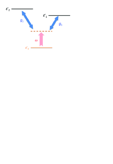
Figure 2: Schematic diagram of a dimer with a laser pulse applied. In the rotating frame, the ground state $\left|\varepsilon_{0}^{(1)}\right\rangle$ is lifted to $\varepsilon_{0}^{\prime}+\omega$. And there are laser-induced transitions between the excited states $\left|\varepsilon_{k}^{(1)}\right\rangle$ and $\left|\varepsilon_{0}^{(1)}\right\rangle$ with coupling strength $g_{k}$.

In the basis of $\left\{\left|\varepsilon_{k}^{(2)}\right\rangle\right\}$ in the rotating frame, the unperturbed and perturbation Hamiltonians read respectively

$$H_{0}^{(2)} = \sum_{k=0}^{2}\left[\varepsilon_{k}^{\prime\prime}+H_{B}+\sum_{n=1}^{2}u_{n}a_{kk}^{(2)}(n)\right]\left|\varepsilon_{k}^{(2)}\right\rangle\left\langle\varepsilon_{k}^{(2)}\right|,$$

$$V^{(2)} = \sum_{k=0}^{2}\sum_{k^{\prime}=0\left(\neq k\right)}^{2}\sum_{n=1}^{2}u_{n}a_{kk^{\prime}}^{(2)}(n)\left|\varepsilon_{k}^{(2)}\right\rangle\left\langle\varepsilon_{k^{\prime}}^{(2)}\right|,$$ (29)

where

$$a_{kk^{\prime}}^{(2)}(n) = \sum_{k_{1}=0}^{2}C_{kk_{1}}^{(2)*}C_{k_{1}n}^{(1)*}\sum_{k_{2}=0}^{2}C_{k^{\prime}k_{2}}^{(2)}C_{k_{2}n}^{(1)}.$$ (30)

Following the CMRT approach, we could obtain the master equation

$$\partial_{t}\rho^{\mathrm{T}}=-\rmi\sum_{k,k^{\prime}}\left(\varepsilon_{k}^{(2)}-\varepsilon_{k^{\prime}}^{(2)}\right)\rho_{kk^{\prime}}^{\mathrm{T}}\left|\varepsilon_{k}^{(2)}\right\rangle\left\langle\varepsilon_{k^{\prime}}^{(2)}\right|$$

$$-\frac{1}{2}\sum_{k,k^{\prime}}\left[R_{k^{\prime}k}^{(2)\textrm{dis}}(t)\rho_{kk}^{\mathrm{T}}\left|\varepsilon_{k}^{(2)}\right\rangle\left\langle\varepsilon_{k}^{(2)}\right|-R_{kk^{\prime}}^{(2)\textrm{dis}}(t)\rho_{k^{\prime}k^{\prime}}^{\mathrm{T}}\left|\varepsilon_{k^{\prime}}^{(2)}\right\rangle\left\langle\varepsilon_{k^{\prime}}^{(2)}\right|\right]$$

$$-\sum_{k,k^{\prime}}\left\{R_{kk^{\prime}}^{(2)\textrm{pd}}(t)+\frac{1}{2}\sum_{k^{\prime\prime}}\left[R_{k^{\prime\prime}k}^{(2)\textrm{dis}}(t)+R_{k^{\prime\prime}k^{\prime}}^{(2)\textrm{dis}}(t)\right]\right\}\rho_{kk^{\prime}}^{\mathrm{T}}\left|\varepsilon_{k}^{(2)}\right\rangle\left\langle\varepsilon_{k^{\prime}}^{(2)}\right|,$$ (31)

where $\rho^{\mathrm{T}}(t)=U^{\dagger}\rho(t)U$ is the density matrix in the rotating frame,

$$\varepsilon_{k}^{(2)} = \varepsilon_{k}^{\prime\prime}-\Lambda_{k}^{(2)},$$ (32)

$$\Lambda_{k}^{(2)} = \sum_{n=1}^{2}\left[a_{kk}^{(2)}(n)\right]^{2}\lambda_{n}.$$ (33)

Here $\varepsilon_{k}^{(2)}$ can be viewed as the eigen value of the electronic Hamiltonian

$$H_{e}^{(2)} = \sum_{k}\varepsilon_{k}^{(2)}\left|\varepsilon_{k}^{(2)}\right\rangle\left\langle\varepsilon_{k^{\prime}}^{(2)}\right|.$$ (34)

In (31), the dissipation rate $R_{kk^{\prime}}^{(2)\textrm{dis}}\left(t\right)$ and pure-dephasing rate $R_{kk^{\prime}}^{(2)\textrm{pd}}(t)$ can be obtained following (17) and (21) by substituting $\varepsilon_{k}^{(1)}$, $\Lambda_{k}^{(1)}$, $g_{k_{1}k_{2}k_{3}k_{4}}^{(1)}(t)$, $\lambda_{k_{1}k_{2}k_{3}k_{4}}^{(1)}$ respectively with $\varepsilon_{k}^{(2)}$, $\Lambda_{k}^{(2)}$,

$$g_{k_{1}k_{2}k_{3}k_{4}}^{(2)}(t) = \sum_{n}a_{k_{1}k_{2}}^{(2)}(n)a_{k_{3}k_{4}}^{(2)}(n)g_{n}(t),$$ (35)

$$\lambda_{k_{1}k_{2}k_{3}k_{4}}^{(2)} = \sum_{n}a_{k_{1}k_{2}}^{(2)}(n)a_{k_{3}k_{4}}^{(2)}(n)\lambda_{n}.$$ (36)

Thus, the influence of the laser field can be considered as modifying the electronic part of the Hamiltonian by pulse induced couplings between ground state and single-excitation states in the rotating frame. Notice that due to the transformation, the density matrix in the original frame $\rho(t)$ is transformed to $\rho^{\mathrm{T}}(t)=U^{\dagger}\rho(t)U$. Hence, after solving the master equation, the obtained density matrix should be transformed back to the original frame as $\rho(t)=U\rho^{\mathrm{T}}(t)U^{\dagger}$. We further remark that (31) enables us to simulate field-induced and dissipative dynamics for an excitonic system due to a step-function pulse. However, this is not a limitation because of the time-local nature of the equations of motion. Within any propagation scheme based on discrete time steps, this formalism can be easily generalized to arbitrary pulse shapes as discussed in A.

2.3 Lindblad-form Coherent Modified Redfield Theory

We have obtained the CMRT master equation that governs the dynamics of an excitonic system in the presence of laser fields. For a system with $M$ chromophores, the CMRT master equation corresponds to a set of $M^{2}$ ordinary differential equations. As a consequence, it would be a formidable task to propagate the dynamics if the system has hundreds of sites, just as in a typical photosynthetic complex, e.g., 96 chlorophylls in PSI. We can apply the NMQJ method [31, 32] to reduce the computational complexity to the order of $M$ to achieve efficient simulation of the CMRT dynamics. The NMQJ method propagates a set of equations of motion in the generalized Lindblad form [49]:

$$\partial_{t}\rho = -\rmi[H_{e}(t),\rho]-\frac{1}{2}\sum_{k,k^{\prime}}R_{kk^{\prime}}(t)\left[\left\{A_{kk^{\prime}}^{\dagger}(t)A_{kk^{\prime}}(t),\rho\right\}-2A_{kk^{\prime}}(t)\rho A_{kk^{\prime}}^{\dagger}(t)\right].$$ (37)

Thus, in order to solve the master equation (cf. (13) and (31)) by means of the NMQJ method, we should rewrite them in the generalized Lindblad form. To this end, we define the following jump operators

$$A_{kk^{\prime}}(t)=\left|\varepsilon_{k}(t)\right\rangle\left\langle\varepsilon_{k^{\prime}}(t)\right|,$$ (38)

where $\left|\varepsilon_{k}(t)\right\rangle$ is $k$th eigen state of the system Hamiltonian $H_{e}(t)$, and the matrix elements of the population transfer and dephasing rates are defined respectively as

$$R_{kk^{\prime}} \equiv \cases{R_{kk^{\prime}}^{\textrm{dis}},&{for} $k\neq k^{\prime}$,\\ \Gamma_{k},&{for} $k=k^{\prime}$,}$$ (39)

where $\Gamma_{k}$s are determined by the pure-dephasing rates in the CMRT master equation:

$$\Gamma=B^{-1}A,$$ (40)

where the matrix elements of $A$ and $B$ are respectively

$$A_{a}=\sum_{k=a+1}^{M}R_{ak}^{\textrm{pd}}+\sum_{k=1}^{M-1}R_{ka}^{\textrm{pd}},$$ (41)

$$B_{jk}=\cases{\frac{1}{2},&{for} $k<j$,\\ \frac{1}{2}(2M-j),&{for} $k=j$,\\ 1,&{for} $j<k<M$,\\ \frac{1}{2},&{for} otherwise.}$$ (42)

Note that since there are $M(M-1)/$2 independent pure-dephasing rates $R_{kk^{\prime}}^{\textrm{pd}}$ in the CMRT master equation and only $M$ Lindblad-form dephasing rates $\Gamma_{k}$, the problem is overdetermined. We found that a least-square fit of $\Gamma_{k}$ to $R_{kk^{\prime}}^{\textrm{pd}}$ preserves the CMRT dynamics extremely well and is also numerically straightforward to implement. The details of the numerical determination of Lindblad-form dephasing rates are presented in B.

3 Non-Markovian Quantum Jump Method

We apply the non-Markovian quantum jump (NMQJ) approach proposed by Piilo et al. to simulate the CMRT equation of motion for multilevel systems [31, 32]. The original implementation of the NMQJ approach only considers a time-independent Hamiltonian. In order to apply the NMQJ method to simulate CMRT dynamics under the influence of laser fields, here we briefly describe the NMQJ method and show how to explicitly implement the method for the time-dependent case to propagate the quantum dynamics of an $M$-level system under the influence of external time-dependent fields.

In our theoretical investigation, we consider the system to be initially in the ground state $\left|\psi_{M}(0)\right\rangle=\left|G\right\rangle$ and thus the initial density matrix is

$$\rho(0)=\left|\psi_{M}(0)\right\rangle\left\langle\psi_{M}(0)\right|.$$ (43)

Then, the laser is turned on and applied to the system for a duration $\tau$ starting at $t=0$. According to the NMQJ method, for an $M$-level system, there are $M+1$ possible states for the system to propagate in, i.e., $\left|\varepsilon_{k}^{(2)}\right\rangle$ for $k=0,1,\cdots M-1$, in addition to the deterministic evolution

$$\left|\psi_{M}^{\mathrm{T}}(t+\delta t)\right\rangle=e^{-\rmi H(t)\delta t}\left|\psi_{M}^{\mathrm{T}}(t)\right\rangle\left\|e^{-\rmi H(t)\delta t}\left|\psi_{M}^{\mathrm{T}}(t)\right\rangle\right\|^{-1},$$ (44)

where the non-Hermitian Hamiltonian is

$$H(t)=H_{e}(t)-\frac{\rmi}{2}\sum_{k,k^{\prime}}R_{kk^{\prime}}(t)A_{kk^{\prime}}^{\dagger}(t)A_{kk^{\prime}}(t).$$ (45)

If $N$ ensemble members are considered in the simulation, the NMQJ method describes the number of ensemble members in each of the individual states at time $t$, $N_{\alpha}^{(\mathrm{I})}(t)$ ($\alpha=0,1,\cdots M$), with the initial value given as

$$N_{\alpha}^{(\mathrm{I})}(0)=\cases{0,&{for} $\alpha=0,1,\cdots M-1$,\\ N,&{for} $\alpha=M$.}$$ (46)

During the pulse duration, the Lindblad-form master equation (31) is solved by the NMQJ method to obtain the distribution of $N_{\alpha}^{(\mathrm{I})}(t)$. Therefore, the density matrix in the rotating frame is straightforwardly given by

$$\rho^{\mathrm{T}}(t)=\frac{1}{N}\left[\sum_{k=0}^{M-1}N_{k}^{(\mathrm{I})}(t)\left|\varepsilon_{k}^{(2)}\right\rangle\left\langle\varepsilon_{k}^{(2)}\right|+N_{M}^{(\mathrm{I})}(t)\left|\psi_{M}^{\mathrm{T}}(t)\right\rangle\left\langle\psi_{M}^{\mathrm{T}}(t)\right|\right].$$ (47)

At the end of the pulse, we transform the density matrix back to the original frame by $\rho(\tau)=U(\tau)\rho^{\mathrm{T}}(\tau)U^{\dagger}(\tau)$ to yield

$$\left|\psi_{M}(\tau)\right\rangle=U(\tau)\left|\psi_{M}^{\mathrm{T}}(\tau)\right\rangle=\beta_{0}e^{\rmi\omega\tau}\left|\varepsilon_{0}^{(1)}\right\rangle+\sum_{k=1}^{M-1}\beta_{k}\left|\varepsilon_{k}^{(1)}\right\rangle,$$ (48)

where $\beta_{k}$s are the expanding coefficients in the basis $\left\{\left|\varepsilon_{k}^{(1)}\right\rangle\right\}$.

Following the end of the pulse, the laser field is switched off and the system then evolves free of laser pulse influence, yet still follows the CMRT master equation describing population relaxation and dephasing in the exciton basis. In this case, since $\left|\varepsilon_{k}^{(2)}\right\rangle$ are not the eigen states of $H_{e}^{(1)}$, we must expand the space of jump states and initialize $M$ new states, i.e., for $k=0,1,\cdots M-1$,

$$\left|\psi_{k+M+1}(\tau)\right\rangle = U(\tau)\left|\varepsilon_{k}^{(2)}\right\rangle=C_{k0}^{(2)}e^{\rmi\omega\tau}\left|\varepsilon_{0}^{(1)}\right\rangle+\sum_{k^{\prime}=1}^{M-1}C_{kk^{\prime}}^{(2)}\left|\varepsilon_{k^{\prime}}^{(1)}\right\rangle,$$ (49)

Thus, to describe both laser-induced dynamics and dissipative dynamics of an excitonic system with $M$ chromophores, we must consider $2M+1$ possible states for the system to propagate in, i.e., $\left|\varepsilon_{k}^{(1)}\right\rangle$ for $k=0,1,\cdots M-1$, and $\left|\psi_{j}(t)\right\rangle$ for $j=M,M+1,\cdots 2M$. The corresponding numbers of ensemble members in the states $N_{\alpha}^{(\mathrm{II})}$ ($\alpha=0,1,\ldots 2M$) are determined by the NMQJ method to solve the CMRT master equation (13) with the initial values given as

$$N_{\alpha}^{(\mathrm{II})}(\tau)=\cases{0,&{for} $\alpha=0,1,\cdots M-1$,\\ N_{M}^{(\mathrm{I})}(\tau),&{for} $\alpha=M$,\\ N_{\alpha-M-1}^{(\mathrm{I})}(\tau),&{for} $\alpha=M+1,M+2,\cdots 2M$.}$$ (50)

Finally, the density matrix can be calculated from the time-dependent distribution of numbers of ensemble members in states $N_{\alpha}^{(\mathrm{II})}(t)$ as

$$\rho(t)=\frac{1}{N}\left[\sum_{k=0}^{M-1}N_{k}^{(\mathrm{II})}(t)\left|\varepsilon_{k}^{(1)}\right\rangle\left\langle\varepsilon_{k}^{(1)}\right|+\sum_{j=M}^{2M}N_{j}^{(\mathrm{II})}(t)\left|\psi_{j}(t)\right\rangle\left\langle\psi_{j}(t)\right|\right].$$ (51)

We remark that the above procedure can be generalized to simulate arbitrary pulse shape as long as the laser pulses only induce transitions between the ground state and single-excitation states. In this case, the eigen states in the rotating frame are always the superpositions of the ground state and single-excitation states. Therefore, once the instantaneous eigen states are changed due to the change in system-field interaction, $M$ new trajectories will be initialized as the previous eigen states are replaced by the eigen states of the new Hamiltonian. In A we present the numerical details for simulating the interaction between an excitonic system and a laser pulse with arbitrary pulse profile.

The generalization of the combined CMRT-NMQJ method for a system in the presence of laser fields can be easily extended to describe multiple pulses to enable the simulation of $N$-wave-mixing optical experiments. For example, the method described in this work can be applied to calculate third-order response functions [46]. Additionally, since the combined CMRT-NMQJ approach describes the full laser-driven dynamics of a dissipative excitonic system, it can be used together with the density matrix based approach for the calculation of photon-echo signals [50, 51] to evaluate nonlinear spectra, including 2D electronic spectra and photon-echo peakshift signals. Although 2D electronic spectra can not be calculated without 2-exciton manifold, it would be straightforward to generalize the results presented in this work to include dynamics in the two-exciton manifold [34, 50]. As a result, nonlinear spectra for coupled systems, which are often difficult to calculate due to the need to average over static disorder, can be calculated by using the combined CMRT-NMQJ approach. We emphasize that in addition to the favorable system-size scaling due to dynamical propagation in the wavefunction space, this approach benefits from the fact that the average over static disorder can be performed simultaneously with the average over quantum trajectories. Therefore, the combined CMRT-NMQJ method should provide a much more numerically efficient means for the evaluation of nonlinear spectra in large condensed-phase systems.

Note that in addition to the NMQJ method, quantum trajectory methods such as the non-Markovian quantum state diffusion approach [39, 40] offer alternatives to the unraveling of quantum dynamics in light-harvesting systems [33, 52]. In that approach, an integration of memory kernel and a functional derivative of the wavefunction with respect to the noise are required to obtain the stochastic Schrödinger equation. Recently, de Vega has applied the quantum state diffusion approach within the so-called post-Markov approximation to describe non-Markovian dissipative dynamics of a network mimicking a photosynthetic system [52]. However, generally speaking it is not straightforward to unravel a non-Markovian quantum master equation using the quantum state diffusion approach. In this work we aim to focus on the CMRT method, which is a time-local quantum master equation with a generalized Lindblad form. As a result the quantum jump approach proposed by Piilo and coworkers seems to be a natural way to implement the propagation of the time-local CMRT equation. A detailed comparison of the numerical efficiency and domains of applicability of the various quantum jump and quantum trajectory based methods is given in Refs. [41] and [32]. We believe these methods could provide superior numerical performance as well as useful physical insights for EET dynamics in complex and large systems.

4 EET Dynamics of FMO

In the previous sections, by combing the CMRT with the NMQJ method, we have proposed an efficient approach to simulate the EET dynamics of photosynthetic systems in the presence of laser fields. In order to implement the NMQJ method, the master equation obtained by the CMRT is revised in the Lindblad form. Since several approximations are made in order to efficiently simulate the quantum dynamics of a large quantum open system for a broad range of parameters, it is necessary to verify the validity of this new approach for photosynthetic systems.

As a numerical demonstration, in figure 3, we compare the population dynamics of EET in FMO simulated by two different approaches, i.e., the combined CMRT-NMQJ approach and the numerically exact HEOM method from Ishizaki and Fleming [24]. Clearly, the results from the two methods are in good agreement. The combined CMRT-NMQJ method does not only reproduce the coherent oscillations in the short-time regime but is also consistent with the HEOM in the long-time limit. In the short-time regime the oscillations are somewhat suppressed in the case of CMRT-NMQJ approach. This is likely due to the simplification of the pure-dephasing process by the direct projection operations. If more realistic dephasing operators as implemented in [53] is applied to simulate the pure-dephasing process, we would expect a better accuracy from the CMRT-NMQJ approach. However, this additional effort may require much more computational time with only marginal improvements for EET dynamics in photosynthetic systems. Therefore, it is a reasonable tradeoff for numerical efficiency that we adopt the Lindblad-form CMRT and make use of the NMQJ method to simulate quantum dynamics of realistic photosynthetic systems

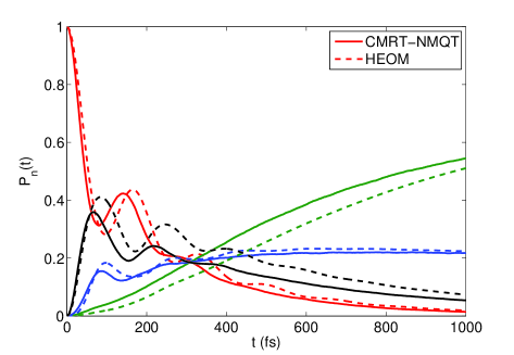
Figure 3: Site population dynamics of FMO with initial excitation on site $6$. The simulation parameters are $T=77$K, $\lambda=35$cm^-1, and the effective Hamiltonian used by Ishizaki and Fleming (cf. [24]) is used in both calculations. Solid curves are obtained by the CMRT-NMQJ approach, and dashed curves depict results from the HEOM method. Red curves are for site $6$, green curves for site $3$, blue curves for site $4$, and black curves for site $5$. In order to make the figure clear, population dynamics for other sites whose populations always stay less than $0.1$ are not shown here.

Note that because the NMQJ is a numerical propagation scheme, the accuracy of the relaxation dynamics calculated by this method actually depends on the Lindblad-form CMRT, which is effectively a generalization to the widely used modified-Redfield theory in terms of population dynamics. Modified-Redfield approach has been proven to provide excellent results for biased-energy systems in photosynthesis [3], therefore we expect the combined CMRT-NMQJ method described in this work to be broadly applicable to EET in photosynthetic systems.

5 Dimer Model

To demonstrate the combined CMRT-NMQJ simulation of laser-driven dynamics, we investigate the behavior of a model dimer system under the influence of laser excitation in this section. Note that in previous simulations of EET dynamics in photosynthetic systems the photoexcitation process was often overlooked and the instantaneous preparation of a given initial condition at zero time is normally assumed. Given that the selective preparation of a specific excitonic state is a highly non-trivial task (in particular the site-localized states often assumed in coherent EET simulations), it is crucial that an experimentally realistic photoexcitation process can be considered in a complete dynamical simulation [27, 28]. Here we show that the combined CMRT-NMQJ approach is capable of describing the excitation process. We further investigate the behavior of a model dimer system (figure 2) under the influence of laser excitation to study the interplay between the laser excitation and ultrafast EET dynamics.

5.1 Absorption Spectrum

Before we examine the laser-induced dynamics we demonstrate that the absorption spectrum can be obtained by the CMRT method (cf. (24)). In figure 4, we show numerically calculated absorption lineshape for dimer system with ground state energy $E_{0}=-12800$cm^-1, site energies $E_{1}=120$cm^-1 and $E_{2}=100$cm^-1, electronic coupling $J=300$cm^-1, and the electronic transition dipole moments in the eigen basis are set to be $\mu_{10}=10$D and $\mu_{20}=5$D, respectively. We further assume identical Ohmic baths described by the spectral density

$$J(\omega)=\lambda\frac{\omega}{\omega_{c}}e^{-\omega/\omega_{c}},$$ (52)

with the reorganization energy $\lambda=35$cm^-1 and the cut-off frequency $\omega_{c}=50$cm^-1, and temperature $T=300$K. The simulated spectrum exhibits two peaks located at $\varepsilon_{2}^{(1)}-\varepsilon_{0}^{(1)}$ and $\varepsilon_{1}^{(1)}-\varepsilon_{0}^{(1)}$, corresponding to the transitions from the ground state $|\varepsilon_{0}^{(1)}\rangle$ to two exciton states $|\varepsilon_{1}^{(1)}\rangle$ and $|\varepsilon_{2}^{(1)}\rangle$.

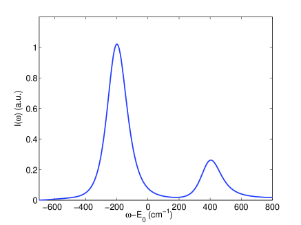
Figure 4: The normalized absorption lineshape for the electronic coupling $J=300$cm^-1, electronic transition dipole moments $\mu_{10}=10$D and $\mu_{20}=5$D, reorganization energy $\lambda=35$cm^-1 and temperature $T=300$K.

Figure 4 shows that the absorption lineshape is well captured by the CMRT approach, which is important if a comparison to experimental data is to be made [36, 47]. The relative peak heights are given by the ratio of $\left|\mu_{k0}\right|^{2}$. Here, the widths of the two peaks are nearly the same as the effect of relaxation-induced broadening is not significant in this particular parameter set. Physically speaking, the pure-dephasing process is much faster than the energy relaxation from the high-energy state $\left|\varepsilon_{2}^{(1)}\right\rangle$ to the low-energy state $\left|\varepsilon_{1}^{(1)}\right\rangle$ when the dimer system is excited. For other cases, the contribution from the relaxation-induced broadening might play a more important role [36].

5.2 Laser-induced Dynamics

In this section, we apply the CMRT-NMQJ approach to investigate the quantum dynamics of a dimer system after laser excitation. As shown in figure 5, the dimer system initially in the ground state is applied with a square laser pulse during the time period $\left[0,t_{1}\right]$. Note that a square pulse is used here for the sake of simplicity (see A). Due to the coupling induced by the laser pulse, the dimer is coherently excited into a superposition between the ground state and the single-excitation states. After the laser is turned off at $t=t_{1}$, the dimer is left alone to evolve under the influence of system-bath couplings. The energy diagrams for the case with and without a laser pulse are depicted in figures 2 and 1, respectively.

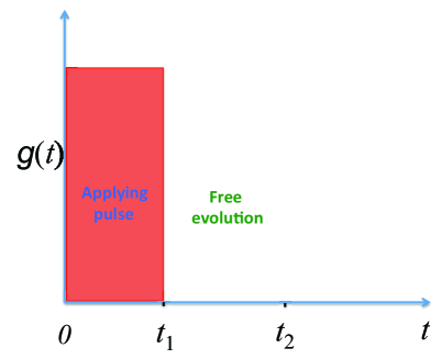
Figure 5: Time sequence of our scheme. The laser is turned on during the period $\left[0,t_{1}\right]$. Afterwards, the laser is turned off and the system is left to evolve free of control.

In our numerical simulation, we adopt the following parameters to model photosynthetic systems: the ground state energy $E_{0}=-12800$cm^-1, the site energies $E_{1}=200$cm^-1 and $E_{2}=100$cm^-1. Moreover, we consider two specific cases $J=120$cm^-1 and $J=20$cm^-1 to explore the electronic coupling’s influence on the dynamics. We further assume identical Ohmic spectral densities (cf. (52)) for each site with a reorganization energy of $\lambda=35$cm^-1, cut-off frequency $\omega_{c}=50$cm^-1, and temperature $T=300$K. In all cases, the laser duration $t_{1}$ is set to $100$fs. In addition, in order to make the results converge within a reasonable computational time, we use a moderate time step $dt=1$fs and average over a sufficiently-large number of trajectories, i.e., $N=10^{5}$.

5.2.1 Laser-induced Population dynamics

Figures 6(a) and 6(b) show the time-evolution of the site populations initialized by a laser pulse for strongly ($J=120$cm^-1) and weakly ($J=20$cm^-1) electronically coupled dimers, respectively. The laser carrier frequency is tuned at $\omega=13000$cm^-1, close to both transition energies. Therefore we expect the laser pulse to induce significant coherence between the two exciton states. As a result, during the pulse duration (from $t=0$fs to $t=100$fs), the populations on both sites oscillate with large amplitudes, for the laser field is nearly on resonance with the transitions between the ground state $|\varepsilon_{0}^{(1)}\rangle$ and two eigen states $|\varepsilon_{1}^{(1)}\rangle$ and $|\varepsilon_{2}^{(1)}\rangle$. After the laser is turned off at $t=100$fs, the population on the ground state remains invariant since there is no relaxation from the single-excitation states to the ground state in our model (cf. (3)), however, dynamics in the single-exciton manifold show strong $J$ dependence. A comparison between figures 6(a) and 6(b) shows that although both systems evolve to reach a thermal equilibrium due to the system-bath couplings, the relaxation dynamics are qualitatively different due to the different electronic coupling strengths. In the case with strong electronic coupling (figure 6(a)) coherent oscillations persist for up to $400$fs, and the system then quickly relaxes to the equilibrium. Clearly, the coherent energy relaxation is extremely efficient in this case and the photoexcitation dynamics and the coherent dynamics are intertwined [54, 42]. We conclude that in strongly coupled systems the nature of the photoexcitation process must be explicitly considered in order to reasonably describe the photon-induced dynamics, as a fictitiously assumed initial condition prepared instantaneously at $t=0$ could not correctly capture the photoexcitation process. In contrast, for the weak electronic coupling case in figure 6(b), the coherent oscillations stop immediately after the pulse is turned off, and the system relaxes incoherently and also slowly. In this case a clear time-scale separation exists and a specific consideration of the photoexcitation process may not be necessary.

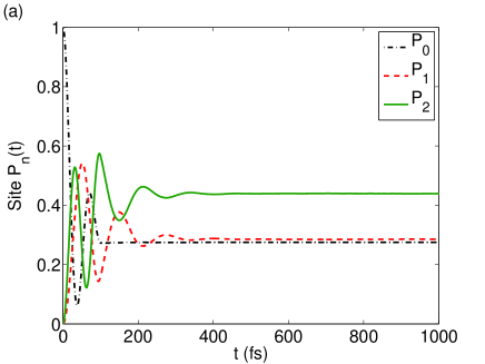
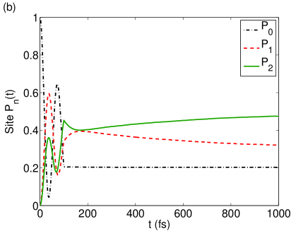
Figure 6: Time evolution of site populations $P_{n}(t)$ for dimer systems interacting with a near-resonant field (a) intradimer electronic coupling $J=120$cm^-1, (b) $J=20$cm^-1. We set the field-induced couplings between the ground state and the two eigen states, $g_{10}=100$cm^-1 and $g_{20}=200$cm^-1.

To investigate the effects of laser excitation condition, we explore the effect of laser detuning on the quantum dynamics in figure 7. In this case, the laser carrier frequency is tuned at $\omega=13400$cm^-1. Because the laser is largely detuned from the transition between $|\varepsilon_{0}^{(1)}\rangle$ and $|\varepsilon_{1}^{(1)}\rangle$ but nearly on resonance with the transition between $|\varepsilon_{0}^{(1)}\rangle$ and $|\varepsilon_{2}^{(1)}\rangle$, i.e., $g_{01}\ll\left|\varepsilon_{1}^{\prime}-\left(\varepsilon_{0}^{\prime}+\omega\right)\right|$ and $g_{02}\sim\left|\varepsilon_{2}^{\prime}-\left(\varepsilon_{0}^{\prime}+\omega\right)\right|$, we expect strong Rabi oscillations for the $|\varepsilon_{0}^{(1)}\rangle\rightleftarrows|\varepsilon_{2}^{(1)}\rangle$ transition, and $|\varepsilon_{1}^{(1)}\rangle$ can not be effectively excited when the pulse is present [55]. Indeed, figure 7(b) shows that in this weak electronic coupling case, site $1$ is selectively excited within the pulse duration, since it is the higher-energy site in our dimer model. Consequently, figure 7(b) indicates that specific initial state, e.g., a specific site being excited, may be prepared if a proper pulse is applied for an appropriate duration. In contrast, figure 7(a) shows that the oscillation amplitudes of site populations, $P_{1}$ and $P_{2}$, are nearly the same in the strong electronic coupling case, as in this case both sites contribute significantly to the delocalized exciton state $|\varepsilon_{2}^{(1)}\rangle$.

Noticeably, the excitation-relaxation dynamics presented in figures 6(a) and 7(a) are markedly different, i.e. no coherent evolution in figure 7(a) after $t=100$fs. Clearly, the dynamical behavior of the strongly coupled dimer depends critically on the excitation conditions. Our results further emphasize the notion that the photoexcitation process must be explicitly considered [27, 28]. Note that we aim to demonstrate the validity of the combined CMRT-NMQJ method developed in this work. It is clear that much more efforts must be paid to elucidate the effects of light source in natural light-harvesting processes. In this regard, the methodology developed in this work appears to be valuable for the study of coherent EET dynamics and quantum coherent control in photosynthetic systems.

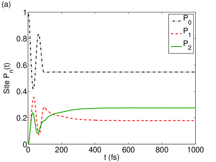
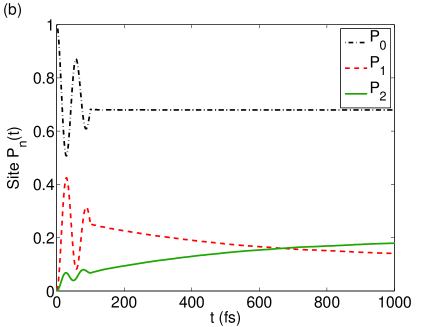
Figure 7: Time evolution of site populations $P_{n}(t)$ for dimer systems interacting with a detuned field with electronic coupling (a) intradimer electronic coupling $J=120$cm^-1, (b) $J=20$cm^-1. We set the field-induced couplings between the ground state and the two eigen states, $g_{10}=40$cm^-1 and $g_{20}=200$cm^-1. The laser frequency is set at $\omega=13400$cm^-1 to be in near resonance with the transition between $|\varepsilon_{0}^{(1)}\rangle$ and $|\varepsilon_{2}^{(1)}\rangle$ but largely-detuned to the transition between $|\varepsilon_{0}^{(1)}\rangle$ and $|\varepsilon_{1}^{(1)}\rangle$.

5.2.2 Entanglement dynamics

In the population dynamics, coherent evolutions are present when the laser excitation or the electronic coupling is strong. To more effectively follow coherent EET dynamics, it has been shown that entanglement is a excellent probe for coherent dynamics in photosynthetic systems [56, 57, 58, 59, 60, 61, 62]. Here, we investigate the time-evolution of entanglement in the dimer system as a demonstration of the combined CMRT-NMQJ method for coherent EET dynamics. Because each pigment in the dimer is a natural qubit, we especially focus on the evolution of concurrence [63]. For a two-qubits system with arbitrary density matrix $\rho$, the concurrence is defined as [63]

$$C\equiv\textrm{max}\left(0,\lambda_{1}-\lambda_{2}-\lambda_{3}-\lambda_{4}\right),$$ (53)

where $\lambda_{j}$s are the square roots of eigen values of the matrix $\rho\tilde{\rho}$ in the descending order. Here,

$$\tilde{\rho}=\left(\sigma_{y}\otimes\sigma_{y}\right)\rho^{*}\left(\sigma_{y}\otimes\sigma_{y}\right)$$ (54)

with $\rho^{*}$ being the complex conjugate of the density matrix $\rho$. For a purely classical system, its concurrence vanishes, while it would be unity for the maximum entangled states, e.g., Bell states. For other states, the concurrence monotonously increases as the state is more quantum-mechanically entangled. An analytical expression that yields $C(t)$ from the matrix elements of $\rho(t)$ can be derived. In our model, since we restrict the evolution of the system within the sub-space without the double-excitation state, the density matrix is of the block type

$$\rho=\left(\begin{array}[]{cccc}0&0&0&0\\ 0&\rho_{22}&\rho_{21}&\rho_{20}\\ 0&\rho_{12}&\rho_{11}&\rho_{10}\\ 0&\rho_{02}&\rho_{01}&\rho_{00}\end{array}\right),$$ (55)

where the basis states are $\left|0\right\rangle=\left|g\right\rangle_{1}\left|g\right\rangle_{2}$, $\left|1\right\rangle=\left|e\right\rangle_{1}\left|g\right\rangle_{2}$, $\left|2\right\rangle=\left|g\right\rangle_{1}\left|e\right\rangle_{2}$, and $\left|3\right\rangle=\left|e\right\rangle_{1}\left|e\right\rangle_{2}$. Thus, the concurrence is simplified as

$$C(\rho) = \max\left\{0,\sqrt{\rho_{11}\rho_{22}}+\left|\rho_{21}\right|-\left(\sqrt{\rho_{11}\rho_{22}}-\left|\rho_{21}\right|\right)\right\}$$ (56)

$$= 2\left|\rho_{21}\right|.$$

Because $\rho_{11}+\rho_{22}\geq 2\left|\rho_{21}\right|$, the more population is excited to the single-excitation states, the larger the concurrence could be. In addition, at some time, when $\rho_{21}$ vanishes, we would expect the system evolves into the disentangled state as the concurrence disappears.

In figure 8, we plot concurrence dynamics for the condition that the excitation pulse is in near resonance with both transitions. For both strong and weak electronic coupling cases, there exists significant entanglement induced by the optical excitation. However, the concurrence dynamics after the laser is switched off at $100$fs are markedly different. Figure 8(a) shows that for the strongly coupled dimer the concurrence quickly evolves to reach a steady state with a considerable value as a result of the large electronic coupling. In contrast, for the weak electronic coupling case shown in figure 8(b), the concurrence rapidly decays to near zero and then follows by a continuous but slow rise. These results are consistent with the characteristics of population dynamics as shown in figure 6, indicating that the concurrence provides an effective tool to describe coherent energy transfer process.

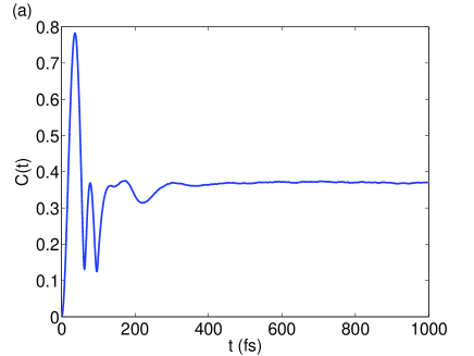
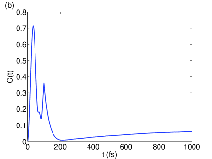
Figure 8: Time evolution of concurrence $C(t)$ for dimer systems interacting with a near-resonant pulse. (a) intradimer electronic coupling $J=120$cm^-1, (b) $J=20$cm^-1. Other parameters are the same as those in figure 6.

Moreover, the evolution of concurrence with only one exciton state selectively excited is shown in figure 9. In the duration of pulse, the maximum entanglement generated by the field is significantly smaller than that by a resonance field. This is because less coherence between the two transitions can be created as a consequence of the laser de-tuning. In addition, because the laser is only in close resonance with one of the transitions, as shown in figure 9(a), the concurrence at the steady state is less than that achieved in figure 8(a), as less population can be excited to the single-excitation states by the weaker pulse. This discovery again emphasizes the importance of the state preparation by photoexcitation.

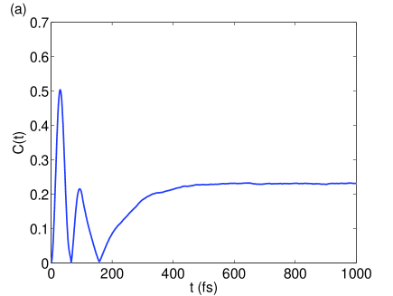
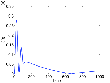
Figure 9: Time evolution of concurrence $C(t)$ for dimer systems interacting with a detuned pulse. (a) intradimer electronic coupling $J=120$cm^-1, (b) $J=20$cm^-1. Other parameters are the same as those in figure 7.

Besides, we notice that for all cases there is an abrupt change at $t=100$fs due to the discontinuity of the system-field interaction, which is an artifact of the step-function pulse shape. We remark that this problem can be solved by using a smooth pulse profile. In a realistic experiment, a gaussian pulse should be applied to the system. The combined CMRT-NMQJ approach can be generalized to consider a gaussian pulse by decomposing it into a series of rectangular sub-pulses with equal width (see details in A). Again, these results indicate that the photoexcitation process plays an important role in the induction of initial coherence in excitonic systems, therefore system-field couplings must be explicitly considered in order to elucidate electronic quantum coherence effects in photosynthesis [28, 14].

6 Conclusions

In this paper, we have combined the CMRT [30] approach and the NMQJ method [31, 32] to develop a formalism that provides efficient simulations of coherent EET dynamics of photosynthetic complexes under the influence of laser fields. In order to implement the NMQJ propagation of the CMRT master equation, the original CMRT master equation is revised in the Lindblad form. In addition, the NMQJ approach is generalized to be suitable for the case with a time-dependent Hamiltonian due to interactions with laser fields. These new developments allow the efficient calculation of quantum dynamics of photosynthetic complexes in the presence of laser fields.

To demonstrate the effectiveness and efficiency of this new approach, we apply the CMRT-NMQJ approach to simulate the coherent energy transfer dynamics in the FMO complex, and compare the result to the one obtained by the numerically exact HEOM method. We show that both results are consistent in the long-time and short-time regimes. Furthermore, we investigate photon-induced dynamics in a dimer system. For strongly coupled dimers, coherent oscillations are observed in the population dynamics during the pulse duration as well as the free evolution as predicted by theory. In addition to the quantum dynamics in the excited states, we also consider coherent effects induced by the laser detuning in the stage of state preparation. We show that the dynamical behavior of a strongly coupled dimer depends critically on the excitation conditions, which further emphasizes the point that the photoexcitation process must be explicitly considered in order to properly describe photon-induced dynamics in photosynthetic systems. In addition, we investigate the evolution of concurrence of a dimer in the presence of laser fields. These results demonstrate the combined CMRT-NMQJ approach is capable of simulation of EET in photosynthetic complexes under the influence of laser control. Note that although the phases of the fields are fixed in our calculations, the combined CMRT-NMQJ method is fully capable of describing quantum coherent control phenomena by shaping phases of the laser fields.

Compared to other numerical simulation methods, this new approach has several key advantages. First of all, because it is based on the CMRT, its validity in a broad range of parameters has been well characterized [3, 30], which is confirmed in simulating the energy transfer dynamics of the FMO complex. Note that the CMRT might fail in the regime where the exciton basis is not a suitable choice [3], e.g., $\lambda>J>\Delta\varepsilon$. In that case, a combined Redfield-Förster picture could be used to provide accurate simulations of EET dynamics [64, 65]. Because the generalized Förster dynamics only add diagonal population transfer terms between block-delocalized exciton states, which directly fit into a Lindblad form, an extension of the methods describe here to simulate EET dynamics in the Redfield-Förster picture will be straightforward. Second, as this approach incorporates the NMQJ method, it effectively reduces the calculation time [31] and therefore is capable of simulating the quantum dynamics in large photosynthetic systems. For an $M$-level system in the absence of laser fields, the effective ensemble size $N_{\mathrm{eff}}=M+1$ in the CMRT-NMQJ approach can be sufficiently smaller than that needed in the non-Markovian quantum state diffusion, e.g. $N=10^{4}$ for a two-level system in Ref. [40]. In addition, the problem of positivity violation, which may be encountered by master equation approaches, can be resolved by turning off the quantum jump once the population of the source state vanishes. Third, it can make use of parallel computation, because the sampling of trajectories can be efficiently parallelized, and it can take the average over static disorder at the same time as the average over trajectories. Finally, since the absorption spectrum [36] and other nonlinear optical signals should be efficiently simulated within the same theoretical framework, all the parameters used in the simulation can be self-consistently obtained by fitting the experimental data using this theoretical approach.

Our motivation to extend the CMRT theory to include time-dependent fields and NMQJ propagation is to provide a tool for the study of quantum control of photoexcitation and energy flow. In order to simulate EET dynamics in a coherent control experiment, it is necessary to consider a time-dependent Hamiltonian that includes the influence of control laser fields. Quantum coherent control lies at the heart of human’s exploration in the microscopic world [66, 67, 68]. Its amazing power manifests in manipulating quantum dynamics by systematic control design methods [69, 70, 71, 72]. The strong motivation to apply quantum coherent control to EET lies in not only the aspiration to knowledge but also the energy need to learn from the highly-efficient photosynthetic systems to improve artificial light harvesting. We believe the methodologies presented in this work would be useful for further investigation of using coherent quantum control methods to direct energy flow in photosynthetic as well as artificial light-harvesting systems. For example, we are currently using the theoretical framework described in this work to investigate how laser pulse-shape and -phase affect EET dynamics in photosynthetic systems.

Appendix A NMQJ Propagation with Arbitrary Pulse Shapes

In Sec. 2.2, we presented the revised CMRT for the case with a step-function pulse. However, in a realistic case, one more often encounters a gaussian pulse. Because the NMQJ approach propagates the dynamics in discrete time intervals, it is trivial to generalize the short-time square pulse propagation scheme given in Sec. 2.2 to treat the influence of a laser pulse with arbitrary pulse profiles.

In figure 10, we schematically demonstrate how to decompose a gaussian pulse with profile $g(t)=g_{0}\exp\left[-2\left(t-t_{0}\right)^{2}/T^{2}\right]$ into $N_{p}$ rectangular sub-pulses with equal width $\Delta T$. The height of each sub-pulse is set to the strength of the gaussian pulse right at the middle of the sub-pulse. The width $\Delta T$ is determined in such a way that by increasing the number of sub-pulses and keeping the duration $[t_{0}-T,t_{0}+T]$ to be fixed, i.e., $N_{p}=2^{n}+1$ ($n=1,2,\cdots$) and $N_{p}\Delta T=2T$, the area difference between the gaussian pulse and the total summation of all sub-pulses does not exceed a pre-determined accuracy threshold. During the time propagation, when the Hamiltonian switches to the case with a different sub-pulse, $M$ new trajectories are added to the propagation. At the end of the sub-pulse sequence, there will be $N_{p}M$ states to propagate in the simulation, which still maintains the linear scaling of the method. For instance, when the gaussian pulse is decomposed into $N_{p}=513$ rectangular sub-pulses, the relative error between the areas of the discretized pulse and the original Gaussian pulse is less than $10^{-6}$, and the total number of states in the propagation only increases linearly to $514M+1$. We remark that the above decomposition procedure holds for arbitrary pulse shapes.

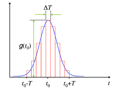
Figure 10: Schematic diagram for decomposing a gaussian pulse centered at $t_{0}$ with width $T$ into $N_{p}$ rectangular sub-pulses with equal width $\Delta T$.

Appendix B Lindblad Form CMRT Mater Equation

In this appendix, we show that (13) can be recast into the generalized Lindblad form. First of all, inspired by the discussion in [31, 32], we shall specifically show that the pure-dephasing term in the CMRT can be rewritten in the Lindblad form:

$$-\sum_{k}\frac{\Gamma_{k}}{2}\left[\left\{A_{kk}^{\dagger}A_{kk},\rho\right\}-2A_{kk}\rho A_{kk}^{\dagger}\right] = -\sum_{k\neq k^{\prime}}\frac{\Gamma_{k}+\Gamma_{k^{\prime}}}{2}\rho_{kk^{\prime}}\left|\varepsilon_{k}\right\rangle\left\langle\varepsilon_{k^{\prime}}\right|$$ (57)

$$= -\sum_{k\neq k^{\prime}}R_{kk^{\prime}}^{\textrm{pd}}\rho_{kk^{\prime}}\left|\varepsilon_{k}\right\rangle\left\langle\varepsilon_{k^{\prime}}\right|,$$

where

$$R_{kk^{\prime}}^{\textrm{pd}}(t)=\frac{1}{2}\left(\Gamma_{k}+\Gamma_{k^{\prime}}\right).$$ (58)

Here, we have made use of the properties of the diagonal jump operators, i.e.,

$$A_{kk}^{\dagger}A_{kk}=A_{kk}^{\dagger}=A_{kk}.$$ (59)

Clearly, the elements of the pure dephasing rate matrix, $R_{kk^{\prime}}^{\textrm{pd}}(t)$, are real and symmetric with respect to the matrix diagonal. In addition, the diagonal terms vanish, i.e.,

$$R_{kk^{\prime}}^{\textrm{pd}}=\cases{\textrm{real},&{for} $k\neq k^{\prime}$,\\ 0,&{for} $k=k^{\prime}$.}$$ (60)

Since there are $M(M-1)/$2 independent pure-dephasing rates $R_{kk^{\prime}}^{\textrm{pd}}$ but $M$ Lindblad-form dephasing rates $\Gamma_{k}$, we need some additional constraints in order to fit $M$ Lindblad-form dephasing rates $\Gamma_{k}$ from $M(M-1)/$2 independent pure-dephasing rates $R_{kk^{\prime}}^{\textrm{pd}}$. In this work, we propose to use a least-square fit to obtain the Lindblad-form dephasing rates. Therefore, we require the mean-square displacement to be minimal with respect to all the Lindblad rates::

$$\frac{\partial}{\partial\Gamma_{a}}\sum_{k=1}^{M-1}\sum_{k^{\prime}=k+1}^{M}\left[R_{kk^{\prime}}^{\textrm{pd}}-\frac{1}{2}\left(\Gamma_{k}+\Gamma_{k^{\prime}}\right)\right]^{2}=0,$$ (61)

where $a=1,2,\ldots M$. After simplification, we obtain a system of linear equations for the Lindblad-form dephasing rates, that is

$$\frac{1}{2}\sum_{k=1}^{a-1}\Gamma_{k}+\frac{1}{2}(2M-a)\Gamma_{a}+\sum_{k=a+1}^{M-1}\Gamma_{k}+\frac{1}{2}\Gamma_{M} = A_{a},$$ (62)

where the coefficient on the right hand side is

$$A_{a}=\sum_{k=a+1}^{M}R_{ak}^{\textrm{pd}}+\sum_{k=1}^{M-1}R_{ka}^{\textrm{pd}}.$$ (63)

Or equivalently, (62) can be written in a matrix form as

$$B\Gamma=A$$ (64)

with the matrix elements of $B$ given by

$$B_{jk}=\cases{\frac{1}{2},&{for} $k<j$,\\ \frac{1}{2}(2M-j),&{for} $k=j$,\\ 1,&{for} $j<k<M$,\\ \frac{1}{2},&{for} otherwise.}$$ (65)

Therefore, by multiplying both sides with the inverse of $B$, we have

$$\Gamma=B^{-1}A.$$ (66)

Therefore, the original CMRT master equation (cf. (13)) can be written in the Lindblad form as

$$\partial_{t}\rho = -\rmi[H_{e}(t),\rho]-\frac{1}{2}\sum_{k\neq k^{\prime}}R_{kk^{\prime}}^{\textrm{dis}}(t)\left[\left\{A_{kk^{\prime}}^{\dagger}A_{kk^{\prime}},\rho\right\}-2A_{kk^{\prime}}\rho A_{kk^{\prime}}^{\dagger}\right]$$ (67)

$$-\frac{1}{2}\sum_{k}\Gamma_{k}(t)\left[\left\{A_{kk}^{\dagger}A_{kk},\rho\right\}-2A_{kk}\rho A_{kk}^{\dagger}\right],$$

as given in (37).

References

References

- [1] Brixner T, Stenger J, Vaswani H M, Cho M, Blankenship R E and Fleming G R 2005 Nature 434 625–628
- [2] Schlau-Cohen G S, Calhoun T R, Ginsberg N S, Read E L, Ballottari M, Bassi R, van Grondelle R and Fleming G R 2009 J. Phys. Chem. B 113 15352–15363
- [3] Novoderezhkin V I and van Grondelle R 2010 Phys. Chem. Chem. Phys. 12 7352–7365
- [4] Engel G S, Calhoun T R, Read E L, Ahn T K, Mancal T, Cheng Y C, Blankenship R E and Fleming G R 2007 Nature 446 782–786
- [5] Collini E, Wong C Y, Wilk K E, Curmi P M G, Brumer P and Scholes G D 2010 Nature 463 644–647
- [6] Panitchayangkoon G, Hayes D, Fransted K A, Caram J R, Harel E, Wen J, Blankenship R E and Engel G S 2010 Proc. Natl. Acad. Sci. U.S.A. 107 12766–12770
- [7] Cheng Y C and Fleming G R 2009 Annu. Rev. Phys. Chem. 60 241–262
- [8] Cao J and Silbey R J 2009 J. Phys. Chem. A 113 13825–13838
- [9] Olaya-Castro A and Scholes G D 2011 Int. Rev. Phys. Chem. 30 49–77
- [10] Jang S and Cheng Y C 2013 WIREs Comput. Mol. Sci. 3 84–104
- [11] Herek J L, Wohlleben W, Cogdell R J, Zeidler D and Motzkus M 2002 Nature 417 533–535
- [12] Caruso F, Montangero S, Calarco T, Huelga S F and Plenio M B 2012 Phys. Rev. A 85 042331
- [13] Brüggemann B, Pullerits T and May V 2006 J. Photochem. Photobiol., A 180 322–327
- [14] Ishizaki A and Fleming G R 2012 Annu. Rev. Phys. Chem. 3 333–361
- [15] Dawlaty J M, Ishizaki A, De A K and Fleming G R 2012 Phil. Trans. R. Soc. A 370 3672–3691
- [16] Cao J 2000 J. Chem. Phys. 112 6719–6724
- [17] Ishizaki A and Fleming G R 2009 J. Chem. Phys. 130 234110
- [18] Jang S, Cheng Y C, Reichman D R and Eaves J D 2008 J. Chem. Phys. 129 101104
- [19] Jang S 2011 J. Chem. Phys. 135 034105
- [20] Kolli A, Nazir A and Olaya-Castro A 2011 J. Chem. Phys. 135 154112
- [21] Chang H T and Cheng Y C 2012 J. Chem. Phys. 137 165103
- [22] Tanimura Y 2006 J. Phys. Soc. Jpn. 75 082001
- [23] Jin J, Zheng X and Yan Y 2008 J. Chem. Phys. 128 234703
- [24] Ishizaki A and Fleming G R 2009 J. Chem. Phys. 130 234111
- [25] Jiang X P and Brumer P 1991 J. Chem. Phys. 94 5833–5843
- [26] Hoki K and Brumer P 2011 Procedia. Chem. 3 122–131
- [27] Mancal T and Valkunas L 2010 New J. Phys. 12 065044
- [28] Brumer P and Shapiro M 2012 Proc. Natl. Acad. Sci. U.S.A. 109 19575–19578
- [29] Fassioli F, Olaya-Castro A and Scholes G D 2012 J. Phys. Chem. Lett. 3 3136–3142
- [30] Hwang-Fu Y H, Chen Y T and Cheng Y C in preparation
- [31] Piilo J, Maniscalco S, Harkonen K and Suominen K A 2008 Phys. Rev. Lett. 100 180402
- [32] Piilo J, Harkonen K, Maniscalco S and Suominen K A 2009 Phys. Rev. A 79 062112
- [33] Rebentrost P, Chakraborty R and Aspuru-Guzik A 2009 J. Chem. Phys. 131 184102
- [34] Zhang W M, Meier T, Chernyak V and Shaul M 1998 J. Chem. Phys. 108 7763–7774
- [35] Yang M and Fleming G R 2002 Chem. Phys. 282 163–180
- [36] Novoderezhkin V I, Rutkauskas D and van Grondelle R 2006 Biophys. J. 90 2890–2902
- [37] Novoderezhkin V I, Doust A B, Curutchet C, Scholes G D and van Grondelle R 2010 Biophys. J. 99 344–352
- [38] Plenio M B and Knight P L 1998 Rev. Mod. Phys. 70 101
- [39] Diósi L, Gisin N and Strunz W T 1998 Phys. Rev. A 58 1699
- [40] Strunz W T, Diósi L and Gisin N 1999 Phys. Rev. Lett. 82 1801
- [41] Brun T A 2002 American Journal Of Physics 70 719–737
- [42] Ai Q, Yen T C, Jin B Y and Cheng Y C 2013 J. Phys. Chem. Lett. 4 2577–2584
- [43] Breuer H P and Petruccione F 2002 The Theory of Open Quantum Systems (New York: Oxford University Press)
- [44] Wu J, Liu F, Shen Y, Cao J and Silbey R J 2010 New J. Phys. 12 105012
- [45] Wu J, Liu F, Ma J, Silbey R J and Cao J 2012 J. Chem. Phys. 137 174111
- [46] Mukamel S 1999 Principles of Nonlinear Optics and Spectroscopy (USA: Oxford University Press)
- [47] Renger T and Mueh F 2013 Phys. Chem. Chem. Phys. 15 3348–3371
- [48] Ohta K, Yang M and Fleming G R 2001 J. Chem. Phys. 115 7609
- [49] Breuer H P 2007 Phys. Rev. A 75 022103
- [50] Cheng Y C, Lee H and Fleming G R 2007 J. Phys. Chem. A 111 9499–9508
- [51] Gelin M F, Egorova D and Domcke W 2009 J. Chem. Phys. 131 194103
- [52] de Vega I 2011 J. Phys. B 44 245501
- [53] Makarov D E and Metiu H 1999 J. Chem. Phys. 111 10126
- [54] Chin A W, Datta A, Caruso F, Huelga S F and Plenio M B 2010 New J. Phys. 12 065002
- [55] Scully M O and Zubairy M S 1997 Quantum Optics (UK: Cambridge University Press)
- [56] Caruso F, Chin A W, Datta A, Huelga S F and Plenio M B 2009 J. Chem. Phys. 131 105106
- [57] Caruso F, Chin A W, Datta A, Huelga S F and Plenio M B 2010 Phys. Rev. A 81 062346
- [58] Fassioli F and Olaya-Castro A 2010 New J. Phys. 12 085006
- [59] Hossein-Nejad H and Scholes G D 2010 New J. Phys. 12 065045
- [60] Ishizaki A and Fleming G R 2010 New J. Phys. 12 055004
- [61] Liao J Q, Huang J F, Kuang L M and Sun C P 2010 Phys. Rev. A 82 052109
- [62] Sarovar M, Ishizaki A, Fleming G R and Whaley K B 2010 Nat. Phys. 6 462–467
- [63] Wootters W K 1998 Phys. Rev. Lett. 80 2245–2248
- [64] Novoderezhkin V I, Marin A and van Grondelle R 2011 Phys. Chem. Chem. Phys. 13 17093–17103
- [65] Bennett D I G, Amarnath K and Fleming G R 2013 J. Am. Chem. Soc. 135 9164–9173
- [66] Brif C, Chakrabarti R and Rabitz H 2010 New J. Phys. 12 075008
- [67] Shapiro M and Brumer P 2003 Principles of the Quantum Control of Molecular Processes (Hoboken: John Wiley & Sons)
- [68] Yan Y A and Kühn O 2012 New J. Phys. 14 105004
- [69] Dong D and Petersen I R 2010 IET Control Theory Appl. 4 2651–2671
- [70] D’Alessandro D 2007 Introduction to Quantum Control and Dynamics (CRC Press)
- [71] Wiseman H M and Milburn G J 2010 Quantum Measurement and Control (Cambridge University Press)
- [72] Mabuchi H and Khaneja N 2005 Int. J. Robust Nonlin. 15 647–667