Idealized computational models for
auditory receptive fields††thanks: The support from the Swedish Research Council (contract 2010-4766) is gratefully acknowledged.
Abstract
This paper presents a theory by which idealized models of auditory receptive fields can be derived in a principled axiomatic manner, from a set of structural properties to (i) enable invariance of receptive field responses under natural sound transformations and (ii) ensure internal consistency between spectro-temporal receptive fields at different temporal and spectral scales.
For defining a time-frequency transformation of a purely temporal sound signal, it is shown that the framework allows for a new way of deriving the Gabor and Gammatone filters as well as a novel family of generalized Gammatone filters, with additional degrees of freedom to obtain different trade-offs between the spectral selectivity and the temporal delay of time-causal temporal window functions.
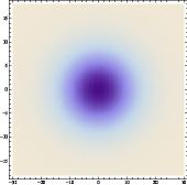
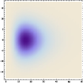
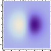
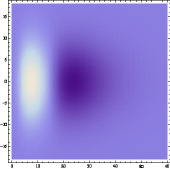
When applied to the definition of a second-layer of receptive fields from a spectrogram, it is shown that the framework leads to two canonical families of spectro-temporal receptive fields, in terms of spectro-temporal derivatives of either spectro-temporal Gaussian kernels for non-causal time or the combination of a time-causal generalized Gammatone filter over the temporal domain and a Gaussian filter over the logspectral domain. For each filter family, the spectro-temporal receptive fields can be either separable over the time-frequency domain or be adapted to local glissando transformations that represent variations in logarithmic frequencies over time. Within each domain of either non-causal or time-causal time, these receptive field families are derived by uniqueness from the assumptions.
It is demonstrated how the presented framework allows for computation of basic auditory features for audio processing and that it leads to predictions about auditory receptive fields with good qualitative similarity to biological receptive fields measured in the inferior colliculus (ICC) and primary auditory cortex (A1) of mammals.
Keywords: receptive field, auditory, temporal, spectro-temporal, scale space, spectrogram, Gabor filter, Gammatone filter, Gaussian derivative, feature detection, onset detection, partial tone detection, glissando, inferior colliculus, primary auditory cortex, auditory perception
Copyright: The Authors
1 Introduction
The information in sound is based on variations in the air pressure over time, which for many sound sources can be modelled as a superposition of sine wave oscillations of different frequencies. To capture this information by auditory perception or signal processing, the sound signal has to be processed over some non-infinitesimal amount of time and in the case of a spectral analysis also over some range of frequencies. Such a region over time or over the spectro-temporal domain is referred to as a temporal or spectro-temporal receptive field [AerJoh81-BICY, TheSenDou-JNeuroSci, MilEscReaSch01-JNeuroPhys, FriShaElhKle03-NatureNeuSci].
If one considers the theoretical or algorithmic problem of designing an auditory system that is going to analyse the variations in air pressure over time, one may ask what types of auditory operations should be performed on the sound signal. Would any operation be reasonable? Specifically, regarding the notion of receptive fields, what types of temporal or spectro-temporal receptive field profiles would be reasonable. Is it possible to derive a theoretical model of how receptive fields “ought to” respond to auditory data?
In vision, the corresponding problem of formulating a theoretical model for visual receptive fields [Lin13-BICY] can be addressed in detail based on a framework developed in the area of computer vision known as scale-space theory [Iij62, Wit83, Koe84, KoeDoo92-PAMI, Lin93-Dis, Lin94-SI, SpoNieFloJoh96-SCSPTH, Flo97-book, Haa04-book, Lin08-EncCompSci, Lin10-JMIV]. A paradigm that has been developed in this field is to impose structural constraints on the first stages of visual processing that reflect symmetry properties of the environment. Interestingly, it turns out to be possible to substantially reduce the class of permissible image operations from such arguments, and it has been shown that biological receptive fields as measured in the lateral geniculate nucleus (LGN) and the primary visual cortex (V1) of higher mammals [HubWie59-Phys, HubWie62-Phys, DeAngOhzFre95-TINS, deAngAnz04-VisNeuroSci, ConLiv06-JNeurSci] can be well modelled by idealized scale-space operations [You87-SV, YouLesMey01-SV, Lin13-BICY, Lin13-PONE].
The subject of this article is to show how a corresponding theory for receptive fields can be developed for auditory stimuli, and how idealized models of auditory receptive fields can be derived by applying scale-space theory to auditory signals. Our aim is to express auditory operations that are well localized over time and frequencies and which allow for well-founded handling of temporal phenomena that occur at different temporal scales as well as receptive fields that operate over different ranges of frequencies in such a way that operations over different ranges of frequencies can be related in a well-defined manner.
It will be shown that when applied to the definition of spectrograms alternatively the formulation of an idealized cochlea model, the scale-space approach can be used for deriving the Gabor [Gab46, WolGodDor01-ASAA, LobLoi03-ICASSP, QiuSchEsc03-JNeuroPhys, WuZhaShi11-ASLP] and Gamma-tone [Joh72-HearTheory, PatNimHolRic87-GammaTone, HewMed94-JASA, PatAllGig95-JASA] approaches for computing local windowed Fourier transforms as specific cases of a complex-valued scale-space transform over different frequencies. In addition, the scale-space approach to defining spectrograms leads to a new family of generalized Gamma-tone filters where the time constants of the individual first-order integrators that are coupled in cascade are not equal as for regular Gamma-tone filters but instead distributed logarithmically over temporal scales and thereby allowing for different trade-offs in terms of e.g. the frequency selectivity of the spectrogram and the temporal delay of time-causal receptive fields.
When applied to a logarithmic transformation of the spectrogram, as motivated from the desire of handling sound signals of different strength (sound pressure) in an invariant manner and with a logarithmic transformation of the frequencies as motivated by the desire of enabling invariance properties under a frequency shift, such as transposing a musical piece by one octave, we will show how this theory also allows for the formulation of spectro-temporal receptive fields at higher levels in the auditory hierarchy in terms of spectro-temporal derivatives of spectro-temporal smoothing operations as obtained from scale-space theory.
It will be demonstrated how such second-layer receptive fields can be used for computing basic auditory features such as onset detection, partial tone enhancement and formants, and specifically how different types of features can be obtained at different temporal scales , spectral scales and how this theory naturally also leads to a glissando parameter that represents how logarithmic frequencies may vary over time according to a local linear approximation .
Compared to the more common approach of computing auditory features in digital signal processing by local windowed fast Fourier transforms (FFT), we argue that proposed theory provides a way to avoid artifacts of performing the computation in temporal blocks that later have to be combined again. Furthermore, by the built-in covariance properties of the model under temporal shifts, variations in sound pressure and frequency shifts, the proposed approach allows for provable invariance properties under such transformations of sound signals.
It will also be shown how idealized models of spectro-temporal receptive fields as obtained from the presented theory in terms of spectro-temporal derivatives of spectro-temporal scale-space kernels can be used for generating predictions of auditory receptive fields that are qualitatively similar to biological receptive fields as measured by cell recordings in the inferior colliculus (ICC) and the primary auditory cortex (A1) [MilEscReaSch01-JNeuroPhys, QiuSchEsc03-JNeuroPhys, MacWehZad04-JNeuroSci, AndLiPol07-JNeuroSci, ElhFriChiSha07-JNeuroSci, AteSch12-PONE].
1.1 Outline of the presentation
The presentation is organized as follows: Section 2 starts by describing basic constraints on temporal receptive fields as motivated by the desire of capturing temporal structures at different temporal scales in a theoretically well-defined manner. Section 3 then describes the temporal scale-space concepts that satisfy these properties, with a distinction on whether the auditory processing operations are required to be time-causal or not. For off-line processing of pre-recorded sound signals, we may take the liberty of accessing the virtual future in relation to any pre-recorded time moment, whereas one in a real-time situation has to take explicit account to the fact that the future cannot be accessed. Thereby, we obtain different theories depending on whether time is treated in a non-causal or a time-causal manner.
In section 4 we apply these temporal scale-space theories to the definition of multi-scale spectrograms by the formulation of local windowed Fourier transforms of different temporal extent to be able to capture temporal phenomena at different temporal scales. Section 5 develops a corresponding theory for spectro-temporal receptive fields applied to the spectrogram, and it is shown how auditory receptive fields over the spectro-temporal domain can be expressed in an analogous way to how visual receptive fields are defined over space-time, with the conceptual difference that the two spatial dimensions in vision are replaced by a logarithmic frequency dimension. Specifically, we demonstrate how basic auditory features can computed in this way from spectro-temporal derivatives of idealized receptive fields as obtained from the auditory scale-space theory.
Section 6 gives examples of how biological auditory receptive fields can be modelled by the proposed theory. Section 7 relates the presented theory to previous approaches in audio processing, and section 8 concludes with a summary and discussion.
Appendix A complements the above treatment by an in-depth analysis of the frequency selectivity properties of the temporal scale-space kernels. Appendix B gives a corresponding analysis of the temporal delays of the time-causal receptive fields. Finally, Appendix C shows how the presented continuous theory can be transferred to a discrete implementation while still preserving the theoretical scale-space properties, and thereby allowing for theoretically well-founded digital implementation.
2 Structural requirements on temporal receptive fields
In the following, we will describe a set of structural requirements that can be stated concerning the temporal receptive fields for a general sensory system that processes a scalar time-dependent signal regarding (i) the measurement of sensory data with its close relationship to the notion of temporal scale, (ii) internal derived representations of the signal that are to be computed by a general sensory system, and (iii) the special nature of time.
If we regard the sensory signal as defined on a one-dimensional continuous temporal axis , then the problem of defining a set of early sensory operations can be formulated as finding a family of operators that are to act on to produce a family of new intermediate representations of the signal111In equation (1), the symbol “” at the position of the first argument of is a place holder to emphasize that in this relation, is regarded as a function and not evaluated with respect to its first argument . The following semi-colon emphasizes the different natures of the temporal coordinate and the filter parameter .
| (1) |
which are also to be defined as functions on , i.e., .
Linearity.
If we want these initial visual processing stages to make as few irreversible decisions as possible, it is natural to initially require to be a linear operator such that
| (2) |
holds for all functions and all scalar constants .
Linearity also implies that a number of special properties of receptive fields (to be developed below) will transfer to temporal derivatives of these and do therefore imply that different types of time-dependent structures in the signal will be treated in a similar manner irrespective of what types of linear filters they are captured by.
Concerning the assumption of linearity, it should be noted that there is an implicit degree of freedom in this formulation concerning the parameterization of the units by which the input signal is measured. Given an underlying measurement signal in units of energy from a sensor, one could for a positive signal also consider defining the input signal in terms of a reparameterization of the sensor signal according to a self-similar power law
| (3) |
for some or using a self-similar logarithmic transformation
| (4) |
defined relative to some reference level . Both of these transformations are self-similar in the sense that (i) they are well-behaved under rescalings of the measurement domain for and (ii) the local magnification/compression around any measurement value as defined from the derivative will also follow a self-similar power law.
Temporal shift invariance.
Let us require to be a shift-invariant operator in the sense that it commutes with the temporal shift operator defined by , such that
| (5) |
holds for all . The motivation behind this assumption is the basic requirement that the representation of a sensory event should be similar irrespective of the time at which it occurs.
Convolution structure.
Together, the assumptions of linearity and shift-invariance imply that the internal representations are given by convolution transformations [HirWid55]
| (6) |
where denotes some family of convolution kernels. These convolution kernels and their temporal derivatives can also be referred to as temporal receptive fields.
Regularity.
To be able to use tools from functional analysis, we will initially assume that both the original signal and the family of convolution kernels are in the Banach space , i.e. that and with the norm
| (7) |
Then also the intermediate representations will be in the same Banach space, and the operators can be regarded as well-defined.
Positivity (non-negativity).
Concerning the convolution kernels , one may require these to be non-negative to constitute smoothing transformations
| (8) |
Normalization.
Furthermore, it is natural to require the convolution kernels to be normalized to unit mass
| (9) |
to leave a constant signal unaffected by the temporal smoothing transformation.
Quantitative measurement of the temporal extent and the temporal offset of non-negative scale-space kernels.
For a non-negative convolution kernel, we can measure the temporal offset by the mean operator
| (10) |
and the temporal extent by the temporal variance
| (11) |
Using the additive properties of mean values and variances under convolution, which hold for non-negative distributions, it follows that
| (12) | |||
| (13) |
Identity operation with continuity.
To guarantee that the limit case of the internal scale-space representations when the scale parameter tends to zero should correspond to the original image data , we will assume that
| (14) |
Hence, the intermediate signal representations can be regarded as a family of derived representations parameterized by a temporal scale parameter .
Semi-group alternatively Markov structure over scale.
For such sensory measurements to be properly related between different temporal scales, it is natural to require the operators with their associated convolution kernels to form a semi-group over
| (15) |
which means that the composition of two convolution kernels from the semi-group should also be a member of the same family of kernels and with added parameters values
| (16) |
Then, the transformation between any different and ordered scale levels and with will obey the cascade property
| (17) |
implying that we can compute the representation at a coarser scale from the representation at any finer scale using a similar type of transformation as when computing the representation at any scale from the original data .
For a temporal scale-space representation based on a discrete set of temporal scale levels with , we can alternatively require a Markov property of the form
| (18) |
where represents the transformation between the adjacent scale levels and . Then, the representation between any pair of temporal scale levels
| (19) |
will be given by convolution with the kernel
| (20) |
The reason for relaxing the semi-group structure to a Markov structure is to make it possible to take larger temporal scale steps at coarser temporal scales, and thereby not requiring the transformations between adjacent temporal scale levels to be equal.
A representation of a signal that possesses these properties is referred to as a temporal multi-scale representation.
Self-similarity over scale.
Regarding the family of convolution kernels used for computing a multi-scale representation, one may require them to self-similar over temporal scales, such that all the kernels correspond to rescaled copies
| (21) |
of some prototype kernel for some transformation222The reason for introducing a function for transforming the scale parameter into a scaling factor over time, is that the requirement of a semi-group structure (15) does not imply any restriction on how the parameter should be related to sound measurements in dimensions of time — the semi-group structure only implies an abstract ordering relation between coarser and finer scales that could also be satisfied for any monotonously increasing transformation of the parameter . For the Gaussian temporal scale-space concept according to equations (27)–(28) this transformation is given by . of of the temporal scale parameter .
Temporal covariance.
If the same sensory stimulus is recorded by two sensors that sample the variations in the signal with different temporal sampling rates, or if similar temporal events occur at a somewhat different speed, it seems natural that the auditory system should be able to relate the temporal scale-space representations that are computed from the data. Therefore, one may require that if the temporal dimension is rescaled by a uniform scaling factor
| (22) |
then there should exist some transformation of the temporal scale parameter such that the corresponding temporal scale-space representations are equal:
| (23) |
In the case of a discrete set of temporal scale levels, we cannot however require self-similarity or temporal covariance to hold exactly. At best, we can aim at approximate transformation properties e.g. in terms of the temporal variance of the temporal scale-space kernels.
Non-creation of new structures with increasing scale.
A necessary requirement on a scale-space representation is that convolution with the scale-space kernel should correspond to smoothing transformation in the sense that coarser scale representations should be guaranteed to constitute simplifications of corresponding finer scale representations.
Non-creation of local extrema (zero-crossings).
One way of formalizing such a requirement for a one-dimensional signal , is by the requirement that the number of local extrema in the data must not increase with scale for any signal and is referred to as non-creation of local extrema. Formally, a one-dimensional kernel is a scale-space kernel if for any signal , the number of local extrema in is guaranteed to not exceed the number of local extrema in [Lin90-PAMI]. It can be shown that for a one-dimensional signal, this condition can also be equivalently expressed in terms of zero-crossings.
For one-dimensional signals, it can be shown that the requirement of non-creation of local extrema implies that a scale-space kernel must be positive and unimodal (having one peak only) both in the spatial domain and the Fourier domain [Lin90-PAMI].
2.1 Specific scale-space axioms for a non-causal temporal domain
Depending on the conditions under which the sensory data is processed, we can consider two types of cases. For pre-recorded signals, we may in principle assume access to the data at all temporal moments simultaneously and thereby apply operations to the signal that would correspond to access to virtual future. For real-time signal processing or when modelling biological perception, there is, however, no way of having access to the future, which imposes fundamental additional structural requirements on a temporal visual front-end. For pre-recorded temporal signals, we require the following:
Non-enhancement of local extrema.
In the case of a continuous scale parameter, one way of formalizing the requirement of non-creation of new image structures with increasing scale is that local extrema must not be enhanced with increasing scale. In other words, if a point is a local (spatial) maximum of the mapping then the value must not increase with scale. Similarly, if a point is a local (spatial) minimum of the mapping , then the value must not decrease with scale. Given the above mentioned differentiability property with respect to scale, we say that the multi-scale representation constitutes a scale-space representation if it for a scalar scale parameter satisfies the following conditions [Lin96-ScSp]:
| (24) | |||
| (25) |
By considering the response to a constant signal, it follows from the requirement of non-enhancement of local extrema that a scale-space kernel should be normalized to unit -norm, corresponding to the normalization requirement in equation (9).
2.2 Special scale-space axioms for a time-causal temporal domain
When processing sensory data in a real-time scenario, the following additional temporal requirements are instead needed:
Temporal causality.
For a sensory system that interacts in with the environment in a real-time setting, a fundamental constraint on the convolution kernels (the temporal receptive fields) is that there is no way of having access to future information, which implies that the temporal smoothing kernels must be time-causal in the sense that the convolution kernel must be zero for any relative time moment that would imply access to the future:
| (26) |
Note that the possibly pragmatic solution of using a truncated symmetric filter of finite support in combination with a temporal delay may not be appropriate for a time-critical real-time system, since it would need to unnecessarily long time delays in particular at coarser temporal scales. Therefore, a dedicated theory for truly time-causal spatio-temporal scale-space concepts is needed.
Time-recursivity.
Another fundamental constraint on a real-time system is that it cannot be expected to keep a full record of everything that has happened in the past. To keep down memory requirements it is therefore desirable that the computations can be based on a limited internal temporal buffer , which should provide:
-
•
a sufficient record of past information and
-
•
sufficient information to update its internal state in a recursive manner over time as new information arrives.
A particularly useful solution in this context is to use the internal temporal representations at different temporal scales as a sufficient memory buffer of the past.
Non-creation of structure in the context of discrete temporal scale levels.
For a temporal scale-space representation involving a discrete set of scale levels only, we build on the requirement of non-creation of local extrema as expressed for a one-dimensional temporal signal depending on time only. Let us therefore regard a one-dimensional temporal smoothing kernel as a temporal scale-space kernel if and only if the kernel is (i) time-causal and in addition (ii) for any purely temporal signal , the number of local extrema in is guaranteed to not exceed the number of local extrema in [LF96-ECCV].
3 Scale-space concepts for purely temporal domains
In this section we will describe how the structural requirements listed in section 2 delimit the class of temporal scale-space kernels and thus the class of possible temporal receptive fields.
3.1 Non-causal Gaussian temporal scale-space
If we for the purpose of analyzing pre-recorded auditory data allow for unlimited freedom of accessing the sensory data at all temporal moments simultaneously, we can apply a similar way of reasoning as has been used for deriving scale-space concepts for image data over a spatial domain [Iij62, Wit83, Koe84, Lin93-Dis, Lin96-ScSp, Flo97-book, WeiIshImi99-JMIV, Haa04-book, Lin08-EncCompSci, Lin10-JMIV].
Given time-dependent sensory data defined over a one-dimensional temporal domain, let us assume that the first stage of sensory processing as represented by the operator should satisfy the following structural requirements: (i) linearity, (ii) shift invariance and (iii) obey a semi-group structure over temporal scales , where we also have to assume (iv) certain regularity properties of the semi-group over scale to guarantee sufficient differentiability properties with respect to time and temporal scales . Let us furthermore require (iv) non-enhancement of local extrema to hold for any smooth function and for any positive scale direction .
Then, it follows from [Lin10-JMIV, theorem 5, page 42] that these conditions together imply that the scale-space family must satisfy a diffusion equation of the form
| (27) |
with initial condition for some positive constant and some constant . Equivalently, this spatio-temporal scale-space representation at scale can be obtained by convolution with temporal Gaussian kernels of the form
| (28) |
with and time and . Since the parameter only corresponds to an unessential rescaling of the temporal scale parameter , we will in the following set .
 |
 |
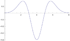 |
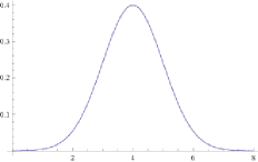
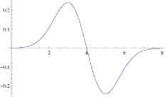
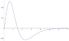
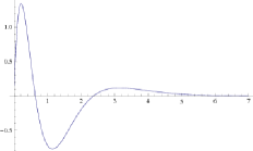
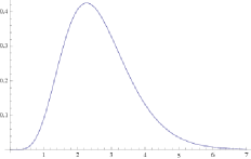
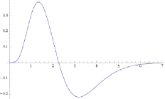
Graphs of these kernels are shown in figure 1. Notably, these kernels are not strictly time causal. To arbitrary degree of accuracy, however, they can be approximated by truncated time-causal kernels, provided that the time delay is chosen sufficiently long in relation to the temporal scale . Hence, the choice of leads to a trade-off between the computational accuracy of the implementation and the temporal response properties as delimited by a non-zero time delay. This problem, however, arises only for real-time analysis. For off-line computations, the time delay can in many cases be set to zero, corresponding to kernels that are mirror symmetric through the origin. In this respect, the truncated and time-shifted Gaussian kernels may serve as a simplest possible model for a temporal scale-space representation, provided that the requirements of temporal causality and temporal recursivity can be relaxed.
Derived receptive fields in terms of temporal derivatives.
In addition to the zero-order smoothing kernel , we have in figure 1 also shown its first- and second-order temporal derivatives and . The reason for this is that derivatives of scale-space kernels do also obey desirable structural properties in terms of linearity, shift invariance and nice properties over scale in terms of non-enhancement of local extrema, with the semi-group property replaced by a cascade property over scale
| (29) |
and with the limit case when the temporal scale goes to zero (14) replaced by
| (30) |
provided that the corresponding derivative of exists. Regarding temporal receptive fields that are expressed in terms of derivatives of scale-space kernels, the normalization condition (9) is replaced by the integral of the receptive field being zero
| (31) |
In all other major respects, such receptive fields satisfy essential scale-space properties in terms of non-creation of new structures with increasing scale in the sense that local extrema in the receptive field response are not enhanced from a fine to a coarser scale or that the number of local extrema or zero-crossings in the signal is guaranteed to not increase from any fine to any coarser scale.
In addition, receptive fields that are expressed in terms of temporal derivatives are invariant under additive transformations of the signal
| (32) |
and thereby providing a mechanism for capturing local variations in the signal under variabilities of its magnitude.
3.2 Time-causal temporal scale-space
When constructing a system for real-time processing of sensory data, a fundamental constraint on the temporal smoothing kernels is that they have to be time-causal. As previously mentioned, the ad hoc solution of using a truncated symmetric filter of finite temporal extent in combination with a temporal delay is not appropriate in a time-critical context. Because of computational and memory efficiency, the computations should furthermore be based on a compact temporal buffer that contains sufficient information for representing sensory information at multiple temporal scales and computing features therefrom. Corresponding requirements are also necessary in computational modelling of biological perception.
Time-causal scale-space kernels for a purely temporal domain.
Given the requirement on a temporal scale-space kernel in terms of non-creation of local extrema over a purely temporal domain, truncated exponential kernels
| (33) |
can be shown to constitute the only class of time-causal scale-space kernels over a continuous domain [Lin90-PAMI, LF96-ECCV]. The Laplace transform of such a kernel is given by
| (34) |
and by coupling such kernels in cascade, we obtain a composed filter
| (35) |
having a Laplace transform of the form
| (36) |
The composed filter has temporal mean value
| (37) |
and temporal variance
| (38) |
In terms of physical models, repeated convolution with this set of truncated exponential kernels corresponds to coupling a series of first-order integrators with time constants in cascade:
| (39) |
with . These temporal smoothing kernels satisfy scale-space properties in the sense that the number of local extrema or the number of zero-crossings in the temporal signal are guaranteed to not increase with the temporal scale. In this respect, these kernels have a desirable and well-founded smoothing property that can be used for defining multi-scale observations over time. A limitation of this type of temporal scale-space representation, however, is that the scale levels are required to be discrete and that the scale-space representation does hence not admit a continuous scale parameter. Computationally, however, the scale-space representation based on truncated exponential kernels can be highly efficient and admits for direct implementation in terms of hardware (or wetware) that emulates first-order integration over time (see figure 2 for illustration of a corresponding electric wiring diagram).

 |
 |
 |
 |
 |
 |
 |
 |
 |
 |
 |
 |
 |
 |
 |
 |
 |
 |
When implementing this temporal scale-space concept, a set of intermediate scale levels has to be distributed between some minimum scale level and some maximum scale level . Assuming that a total number of scale levels is to be used, it is natural to distribute the temporal scale levels according to a geometric series, corresponding to a uniform distribution in units of effective temporal scale [Lin92-PAMI]. Using such a logarithmic distribution of the temporal scale levels, the different levels in the temporal scale-space representation at increasing temporal scales will serve as a logarithmic memory of the past, with qualitative similarity similarity to the mapping of the past onto a logarithmic time axis in the scale-time model by [Koe88-BC]. If we have the freedom of choosing freely, a natural way of parameterizing these temporal scale levels is by using a distribution parameter such that
| (40) |
which by equation (38) implies that time constants of the individual first-order integrators will be given by
| (41) | |||
| (42) |
If the temporal signal is on the other hand given at some minimum temporal scale level , we can instead determine in (40) such that
| (43) |
and add temporal scale levels with according to (42). Alternatively, if one chooses a uniform distribution of the intermediate temporal scale levels
| (44) |
implying
| (45) |
then it becomes straightforward to compute the explicit expression for the composed kernel
| (46) |
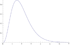
which has temporal mean value and variance . Note that in contrast to the primitive truncated exponentials, which are discontinuous at the origin, these kernels are continuous of order , thus allowing for differentiation up to order . The corresponding expressions for the first- and second-order derivatives are
| (47) | |||
| (48) |
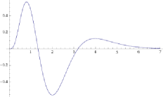
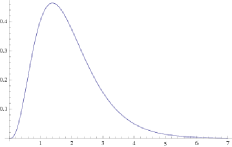
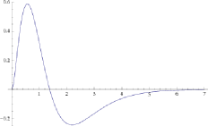
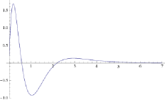
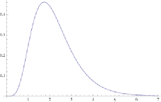
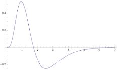
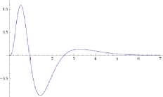
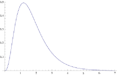
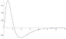
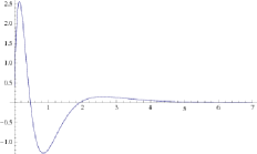
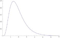
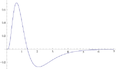
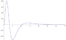
Figure 4 shows graphs of these kernels for two combinations of and that correspond to the same value of the composed variance . As can be seen from the graphs, the kernels are highly asymmetric for small values of , whereas they become gradually more symmetric as increases. Figures 4–5 show corresponding compositions of truncated exponential kernels for self-similar distributions of the intermediate time constants according to equations (40), (41) and (42) for and . As can be seen from a comparison between figure 4 and figures 4–5, the use of a self-similar distribution of the time constants (in figures 4–5) allows for smoother behaviour near the origin with increasing while not increasing the temporal delay as much as for the kernels corresponding to a uniform distribution of the intermediate temporal scale levels (in figure 4).
Time-recursive computation of temporal derivatives.
Temporal scale-space derivatives of order can be defined from this scale-space model according to
| (49) |
where the Laplace transform of the composed (equivalent) derivative kernel is
| (50) |
For this kernel to have a net integration effect, and to enable well-posed derivative operators, an obvious requirement is that the total order of differentiation should not exceed the total order of integration. Thereby, is a necessary requirement. As a consequence, the composed transfer function must have finite -norm.
A very useful observation that can be made concerning derivative computations is that temporal derivatives can equivalently be computed from differences between different temporal channels. Let us first assume that all time constants are different in (50). Then, a partial fraction division gives
| (51) |
where
| (52) |
showing that each temporal derivative can be computed as a linear combination of the representations at the different time-scales.
More realistically, however, the channels that we can regard as available at a certain temporal scale with index will not be the results of direct filtering with different time constants . Rather, we would like to use the intermediate outputs from the cascade coupled recursive filters for . Decomposition of into a sum of such transfer functions
| (53) |
shows that the weights are given as the solution of a triangular system of equations provided that the necessary condition is satisfied
| (54) |
After a few more calculations it can be shown that the Laplace transforms of the equivalent derivative computation kernels satisfy the recurrence relation [LF96-ECCV]
| (55) |
implying that higher-order temporal derivatives can be computed from small-support finite differences of lower-order derivatives (analogous to pure finite differences in the spatial domain) where the temporal scale-space representations at different temporal scales serve as a sufficient temporal buffer of what has occurred in the past. Derivative computations will therefore be highly efficient. Specifically, it follows that both the temporal smoothing operation and the computation of temporal derivatives are time-recursive.
4 Multi-scale spectrograms for auditory signals
The above treatment concerning temporal receptive fields is general and can be used for modelling desirable properties of receptive fields for a variety of time-dependent sensory signals. For auditory signals, an additional structural requirement arises from the fact that the auditory information is transferred in terms of sound waves that travel from the transmitter to the receiver and the auditory information can be encoded in terms of oscillation frequencies of the air pressure that generates the sensory signal. For this reason and from our knowledge that the variations due to the geometry and other properties of the cochlea leads to physical resonances whose effect can be modelled by as a physical Fourier transform, spectrograms are a common tool for analyzing auditory information.
Note that our primary aim is not to specifically model, for example, the measured response of the nerves coming from the cochlea as typically done in previous auditory models [PatAllGig95-JASA]. Instead we are following the scale-space theory using the principle of invariance as outlined in section 2 and section 3.
 |
 |
 |
 |
 |
 |
 |
 |
 |
 |
 |
 |
 |
 |
 |
 |
 |
 |
 |
 |
 |
 |
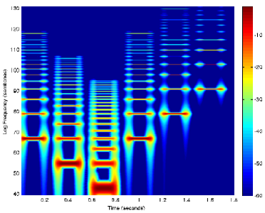
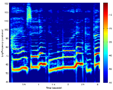
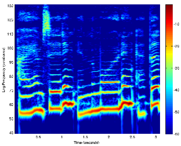
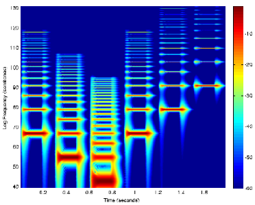
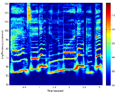
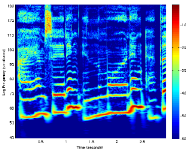
Based on the two models for temporal receptive fields (non-casual in section 3.1 and time-casual in section 3.2), we can use the temporal smoothing functions in these two temporal scale-space models as scale-dependent window functions for defining two types of complex-valued multi-scale spectrograms according to
| (56) | |||
| (57) |
where
-
•
is a temporal Gaussian kernel of the form (28),
-
•
with is the equivalent convolution kernel corresponding to a cascade of truncated exponential filters of the form (35).
These definitions imply that the convolution kernels used for defining temporal scale-space for a general time-varying signal are here used as scale-dependent window functions for defining windowed Fourier transforms of different temporal extent.
For a given value of , the spectrogram becomes a 2-D function. With the definition extended to all values of , the spectrogram based on Gaussian window functions instead becomes a 3-D volume over all temporal extents of the window function or alternatively a set of discrete 2-D slices for the window functions based on truncated exponential functions coupled in cascade for vectors of different length .
Note that a priori there may be no principled reason for preferring a particular duration of the temporal window function for the windowed Fourier transform over some other temporal duration. Specifically, different temporal durations may be appropriate for different auditory tasks, such as a preference for a short temporal duration for onset detection and a preference for a longer temporal duration to separate sounds with nearby frequencies. In this context, the scale-space approach allows for the definition of windowed Fourier transforms for all temporal extents in such a way that any windowed Fourier transforms at a coarse temporal scale can be related to a windowed Fourier transform at any finer scale using the cascade property (17) derived from the semi-group structure (15) or the Markov property (18) of the underlying scale-space kernels. In combination with the additional scale-space properties of non-creation of new structures with increasing scale, this guarantees well-founded theoretical properties between corresponding windowed Fourier transforms computed at different temporal scales.
In most other work on auditory signal processing, there is often an implicit assumption that one chooses a scale for computing the auditory features that seems to work and on which later stage analysis is then based. By the presented formulation of multi-scale spectrograms, we aim at making the consequences of such assumptions explicit, and emphasizing the possibility of computing auditory features at multiple temporal scales as an integrated part of the analysis. Compared to the more traditional approach of computing spectrograms from local fast Fourier transforms combined with local windowing operations, this formulation of multi-scale spectrograms avoids the concatenation of such windowing operations altogether and thereby the artifacts caused by these.
The scale-space approach for defining multi-scale auditory spectrograms implies that instead of computing a scale-space representation of the original auditory signal, the auditory signal is first projected onto the two orthogonal dimensions and of a complex sine wave
| (58) |
for which temporal scale-space representations are then defined, implying that the multi-scale spectrogram can be interpreted as a complex-valued scale-space transform.
Invariance and covariance properties.
Concerning the symmetry requirements of a general temporal sensory front-end described in section 2, the linearity of the scale-space operations is transferred to a linearity in the complex multi-scale spectrograms (56)–(57). This implies that multiple sources of sound will combined in an additive manner in terms of their complex-valued responses and that sound sources of different strength (sound pressure) will be handled in a similar manner up to a multiplication of the strength of the signal.
Regarding temporal shift invariance, the magnitude maps of are invariant under a shift of the temporal axis, whereas the phase of the truly complex spectrograms and will be transformed in a predictable manner between similar sound signals that occur at different time moments or at different distances to the observer.
Under a local rescaling of the temporal axis, the temporal receptive fields obtained from the Gaussian scale-space model are fully scale covariant. Under a rescaling of the temporal axis
| (59) |
the corresponding complex-valued multi-scale spectrograms are transformed according to
| (60) |
If we let the window scale for any angular frequency be proportional to the wavelength corresponding to that frequency, then the corresponding spectrograms within the same 2-D slice of the extended 3-D multi-scale spectrogram can therefore be perfectly matched under a rescaling of the temporal axis corresponding to a frequency shift
| (61) |
If the temporal window functions on the other hand do not have the temporal extent proportional to the wavelength, then temporal covariance does not hold within the same 2-D slice but still holds within the 3-D multi-scale spectrogram based on Gaussian window functions because of their self-similarity over scale, whereas the corresponding scaling relations can only be approximate for the truncated exponential functions coupled in cascade, because of the temporal scale levels being restricted to a discrete set of values.
Again there may not be any principled reason for preferring a particular temporal scale over another. The multi-scale nature of the corresponding spectrogram makes this aspect explicit and opens up for using different temporal scales for different auditory tasks, where different temporal scales may have complementary advantages.
Relations to Gabor functions.
By rewriting the expression (56) for the complex-valued spectrogram based on the Gaussian temporal scale-space concept as
| (62) |
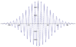
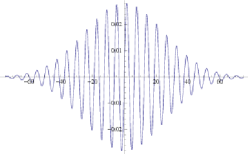
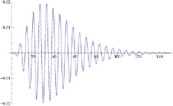
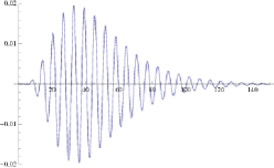
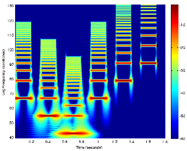
it can be seen that up to a phase shift by this multi-scale spectrogram can equivalently be interpreted as the convolution of the original auditory signal by Gabor functions [Gab46] of the form (see figure 6, top row)
| (63) |
Such Gabor functions have been previously used for analyzing auditory signals by several authors, including [WolGodDor01-ASAA, Kle02-ActAcust, KleGel02-InterSpeech, LobLoi03-ICASSP, QiuSchEsc03-JNeuroPhys, BooLie06-ICASSP, EzzBouPog07-InterSpeech, DomHecJouGoe08-ICASSP, HeLecMadAll09-AffComp, HecDomJouGoe11-SpeechComm, WuZhaShi11-ASLP, SchMeyKol12-JASA, SamLac12-SpeechTech]. Our theory provides a new way of deriving this form of representation with special emphasis on the multi-scale nature of the Gaussian window functions and their resulting cascade properties between spectrograms at different temporal scales.
Relations to Gammatone filters.
In the special case when the time constants of all the truncated exponential filters that are coupled in cascade are all equal , it follows from combination of equations (57) and (46) that the multi -scale spectrogram is given by
| (64) |
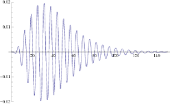
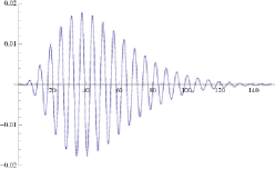
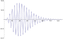
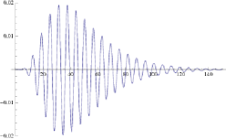
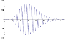
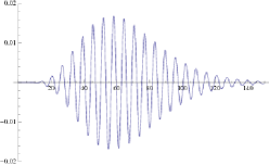
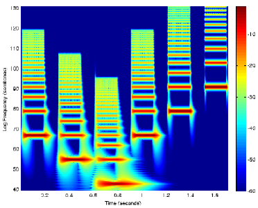
corresponds to convolution of the input signal by filters of the form (see figure 6, third and fifth rows)
| (65) | |||
| (66) |
For comparison, the Gammatone filter with parameters and and frequency is defined according to
| (67) |
By identification of the parameters
| (68) |
and using it follows that we can derive the Gammatone filter as a special case of applying a time-causal scale-space representation with discrete scale levels to the projections and of an auditory signal onto a complex sine wave .
Gammatone filter banks are also commonly used in audio processing [Joh72-HearTheory, PatNimHolRic87-GammaTone, HewMed94-JASA, PatAllGig95-JASA, IriPat97-JASA, AmbEppLin01-ICASSP, Hoh02-GammaTone, ImmPee03-AcResLettOnLine, SchBezWagNey07-ICASSP, NgaSawHisSer10-ISCAS]. The present treatment provides a new way of deriving them in a principled and conceptually similar way as the Gabor filters can be derived, with the differences that the temporal filtering operations are required to be truly time-causal and that only a discrete set of temporal scale levels is to be used.
Generalization of Gammatone filters.
In addition, by allowing for different time constants in the primitive truncated exponential filters, this scale-space concept leads to a generalized family of such kernels
| (69) | |||
| (70) |
with according to (36). As can be seen from a comparison between the two classes of time-causal window functions in figure 6, which are shown for the same temporal extent as measured in terms of the variance of the underlying filter without the complex sine wave, the frequency selective filters based on truncated exponential filters having a logarithmic distribution of the intermediate temporal scale levels allow for a faster response compared to the corresponding filters based on a uniform distribution. Thereby, this family of generalized Gammatone filters allows for additional degrees of freedom to obtain different trade-offs between e.g. the frequency selectivity and the temporal delay of time-causal window functions by varying the number of levels and the distribution parameter — see appendix A and appendix B for in-depth analysis of the frequency selectivity and the temporal delay of such kernels.
Frequency-dependent window scale.
To guarantee basic covariance properties of the spectrogram under a frequency shift
| (71) |
it is as earlier mentioned natural to let the temporal window scale vary with the frequency in such a a way that the temporal window scale in units of is proportional to the wavelength
| (72) |
where is a parameter. Thereby, it follows that e.g. a shift by one octave of a musical piece implies that the corresponding spectrogram will also appear similar while shifted by one octave if the frequency axis of the spectrogram is parameterized on a logarithmic scale.
To prevent the temporal window scale from being too short for high frequency sounds, we have additionally chosen to add a soft lower threshold such that the temporal extent is instead chosen according to
| (73) |
where denotes a lower bound on the temporal window scale. Thereby, frequency covariance of a 2-D spectrogram will only be approximate, while being a good approximation if . If we quantify as , then the soft threshold corresponds to
| (74) |
which with , and corresponds to a frequency of about 4 600 Hz. By varying the parameters and , we can move the frequency where deviations from true invariance begin to occur for a given value of the tolerance parameter .
In human hearing, there is different evidence that the resolution of pitch perception decreases in the area around 2-5 kHz (see e.g. [Har96-JASA]). The frequency difference limen for sine tones decreases [Moo73-JASA]; the synchrony in the neural firing in the auditory nerve decreases [Joh80-JASA], and the ability to identify the pitch of a mistuned harmonic decreases [HarMcAdaSmi90-JASA]. All three effects occur within the same frequency range. Therefore, there should presumable be an upper limit above which self-similarity will not hold.
To prevent the temporal delay from being too long at low frequencies, one can also introduce a soft upper bound on the temporal scale
| (75) |
for suitable values of the parameters and . Then, approximate frequency covariance will hold over some subset of frequencies as defined by the parameters , , and .
5 Receptive fields defined over the spectrogram
Given that a spectrogram has been computed by a first layer of auditory receptive fields, we will define a second layer of receptive fields by operating on the spectrogram with 2-D spectro-temporal filters as illustrated in figure 9, in a structurally similar way as visual receptive fields are applied to time-varying visual input [Lin13-BICY, Lin13-PONE].
| Auditory features |
| Second layer of spectro-temporal receptive fields |
| Transformed spectrogram |
| Self-similar transformations and |
| Multi-scale spectrogram |
| First layer of frequency selective temporal receptive fields |
| Auditory signal |
5.1 Logarithmic transformations of the spectrogram
Prior to the definition of receptive fields from the spectrogram, it is natural to allow for a self-similar transformation of the magnitude values of the spectrogram
| (76) |
A logarithmic transformation of the magnitude values of the spectrogram implies that a multiplicative transformation of the sound pressure , corresponding to , or an inversely proportional reduction in the sound pressure of the signal from a single auditory point source as function of distance , corresponding to , are both transformed into a subtraction of the logarithmic magnitude values by a constant
| (77) |
If we operate on the logarithmically transformed spectrogram by a receptive field that is based on a combination of a spectro-temporal smoothing operation with spectral and temporal scale parameters as determined by a spectro-temporal covariance matrix , spectral and/or temporal derivatives of orders and with at least one of or
| (78) |
then it follows that the influence on the receptive field responses of the constants and
| (79) |
will be eliminated by the derivative operation if the constants and do not depend on time or logarithmic frequency , implying invariance of the second-layer receptive field responses to variations in the sound pressure or the distance to a sound source.
A logarithmic transformation of the magnitude values is also compatible with the Weber-Fechner law, which states that the ratio of an increment threshold of a stimulus for a just noticeable different in relation to the background intensity is constant over large ranges of magnitude variations, which approximately holds in both visual and auditory perception [Pal99-Book, KanSchJes00-PrincNeurSci].
Furthermore, since logarithmic frequencies constitutes a natural metric for relating frequencies of sound [Fle34-JASA, KanSchJes00-PrincNeurSci, You05-JASA] and there is an approximately logarithmic distribution of frequencies both on the basilar membrane [Gre90-JASA] and in the organization of the auditory cortex [RomWilKau82-Science], it is natural to express these derived receptive fields in terms of logarithmic frequencies parameterized by
| (80) |
for some constants and , where specifically and corresponds to logarithmic frequencies according to the MIDI standard.
5.2 Structural requirements on second-layer spectro-temporal receptive fields
Given a transformed spectrogram defined in this way, let us define a family of second layer spectro-temporal receptive fields that are to operate on the transformed spectrogram and be parameterized by some multi-dimensional spectro-temporal scale parameter that includes smoothing over time and logarithmic frequencies , and for which the corresponding operator is required to obey:
-
(i)
linearity over the logarithmic spectrogram
(81) to ensure that (a) the multiplicative relations of the magnitude of the spectrogram (77) that are mapped to linear relations by the logarithmic transformation (76) are preserved as linear relations over the receptive field responses and (b) that scale-space properties that are imposed to ensure non-creation of new structures in smoothed spectrograms as defined by spectro-temporal smoothing kernels do also transfer to spectro-temporal derivatives of these,
-
(ii)
shift-invariance with respect to translations over time and logarithmic frequencies
(82) such that all temporal moments and all logarithmic frequencies are treated in a similar manner. Temporal shift invariance implies that an auditory stimulus should be perceived in a similar manner irrespective of when it occurs. Shift-invariance in the logarithmic frequency domain implies that, for example, a piece of music should be perceived in a similar manner if it is transposed by e.g one octave.
These conditions together imply that the spectro-temporal receptive fields should be given by convolution with some two-dimensional kernel over the spectro-temporal domain [HirWid55]
| (83) |
To characterize what types of receptive fields are compatible with scale-space properties, we will next impose additional structural requirements, which will take different forms depending on time is treated in a time-causal or non-causal manner.
Relations between receptive fields at different spectro-temporal scales.
For pre-recorded sound signals, for which we can take the freedom of accessing data from the virtual future in relation to any time moment, we impose a
-
(iii.a)
continuous semi-group structure over spectro-temporal scales on the second layer of receptive fields
(84) corresponding to an additive structure over the multi-dimensional scale parameter .
For time-causal causal signals, we require:
-
(iii.b)
a continuous semi-group structure over spectral scales
(85) and a Markov property between adjacent temporal scales:
(86)
These requirements are analogous to previous treatment in section 2, with extensions from a purely temporal domain to a spectro-temporal domain.
Non-creation of new spectro-temporal structures with increasing scale.
When processing the spectrogram at different spectro-temporal scales, we want to ensure that the spectro-temporal receptive fields do not create new structures at coarser scales that do not correspond to simplifications of corresponding structures at finer scales. Depending on whether time is treated in a time-causal or non-causal manner, we formalize this conditions in different manners:
-
(iv.a)
For the non-causal Gaussian spectrogram (56), for which temporal causality of the temporal smoothing kernels is disregarded, we require non-enhancement of local extrema in the sense that if for some scale the point is a local maximum (minimum) for the mapping then the value at this point must not increase (decrease) with increasing scale .
-
(iv.b)
For the time-causal spectrogram (57) based on truncated exponential filters coupled in cascade (35), we require: (iv.b1) the smoothing operation over the log-spectral domain to satisfy non-enhancement of local extrema in the sense that if at some log-spectral scale a point is a local maximum (minimum) of the mapping obtained by disregarding the temporal variations, then the value at this point must not increase (decrease) with increasing log-spectral scale , and (iv.b2) the smoothing operation over time to be a time-causal scale-space kernel in the sense that it is guaranteed to not create new local extrema under an increase of the temporal scale parameter .
Glissando covariance.
In musical performance, the frequencies may vary continuously over time in such a way that the fundamental frequency and the harmonics (overtones) are all multiplied by the same time-varying factor . This is in particular prominent in singing, but may occur in all instruments with continuous pitch control. In terms of logarithmic frequencies, we can model a local linearization of this temporal variability as a glissando transformation of the form
| (87) |
analogous to the way spatial image data may be subject to local Galilean transformations over time. Comparing two spectrograms, one with constant frequencies over time and one with linearily varying logarithmic frequencies, the glissando transformation can in operator form be expressed as
| (88) |
for . Specifically, in relation to receptive field responses that are computed over the two domains with spectro-temporal scale parameters and , we may require:
-
(v)
If two local patches of two spectrograms are related by a local glissando transformation, then it should be possible to relate the local spectro-temporal receptive field responses such that
(89) for some transformation of the spectro-temporal scale parameters .
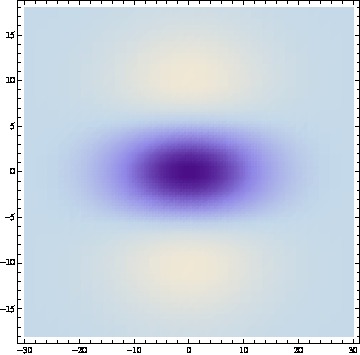
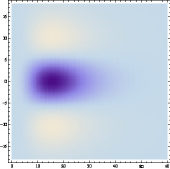
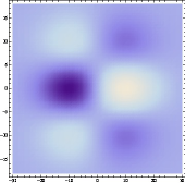
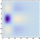
| Gaussian | Time-causal |
| Separable | Separable |
 |
 |
 |
 |
 |
 |
 |
 |
| Glissando-adapted | Glissando-adapted |
 |
 |
5.3 Idealized models for spectro-temporal receptive fields
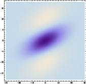
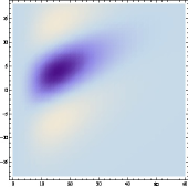
Given the structural requirements above, it can from derivations333The proofs concerning spectro-temporal receptive fields are similar to those regarding spatio-temporal receptive fields over a 1+1-D spatio-temporal domain with the spatial dimension replaced by a spectral dimension. similar to those that are used for constraining visual receptive fields given structural requirements on a visual front-end [Lin13-BICY] be shown that the second layer of auditory receptive fields should be based on spectro-temporal receptive fields of the form
| (90) |
where
-
•
represents a temporal derivative of order with respect to time which could alternatively be replaced by a glissando-adapted temporal derivatives of the form ,
-
•
represents a derivative operator of order with respect to logarithmic frequency ,
- •
-
•
represents a Gaussian smoothing kernel over logarithmic frequencies with spectral scale parameter and representing a glissando parameter that makes it possible to adapt the receptive fields to variations in frequency over time.
Thereby, the spectro-temporal receptive fields according to (90) constitute a combination of the purely temporal receptive fields according to the theory in section 2 and section 3 with a Gaussian scale-space concept over the log-spectral dimension.
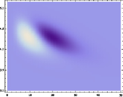
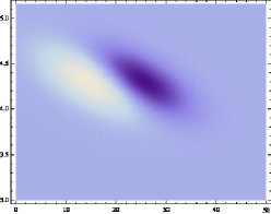
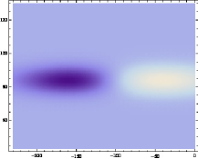
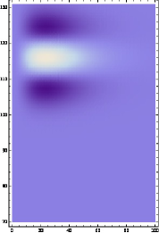
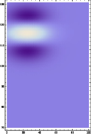
Figure 10 shows examples of spectro-temporal receptive fields obtained in this way for the two different types of underlying temporal scale-space concepts. For , the resulting receptive fields are separable over the spectro-temporal domain, whereas leads to non-separable glissando-adapted spectro-temporal receptive fields.
Filter parameters of auditory receptive fields.
The auditory features that are computed from these types of receptive fields depend on three different scale parameters:
-
•
a temporal window scale parameter defining the temporal extent of the windows over which the windowed Fourier transforms in the spectrograms are defined,
-
•
a secondary temporal integration scale parameter defining the temporal extent over which the magnitude values in the spectogram are integrated over time and
-
•
a spectral scale parameter defining the extent over which smoothing is performed over logarithmic frequencies .
In addition, this class of spectro-temporal receptive fields comprises:
-
•
a glissando parameter that makes it possible to adapt the receptive fields to variations on the logarithmic frequencies over time ,
and each parameterized spectro-temporal receptive field may occur for different orders of differentiation and with respect to time and logarithmic frequencies, respectively.
| Spectrogram: | Spectral smoothing: |
 |
 |
| Transient enhancement: | Onset detection: |
 |
 |
| Spectral band detection: | Spectral band detection: |
 |
 |
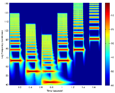
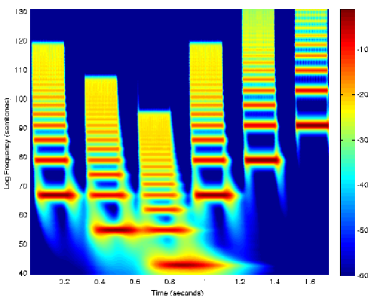
| Spectrogram: | Spectral smoothing: |
 |
 |
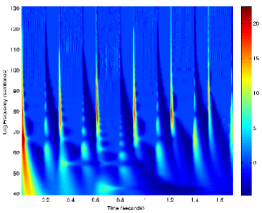
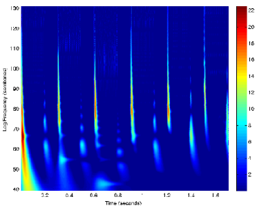
| Transient enhancement: | Onset detection: |
 |
 |
| Spectral band detection: | Spectral band detection: |
 |
 |
 |
 |
 |
| Glissando | Glissando |
 |
 |
| Glissando | Glissando |
 |
 |
| Glissando | Glissando |
 |
 |
5.4 Auditory features from second layer spectro-temporal receptive fields
In the following, we will show examples of auditory features that can be defined from a second layer of auditory receptive fields of this form.
Spectro-temporal smoothing.
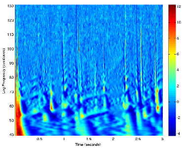
Auditory receptive fields that correspond to convolution with a spectro-temporal smoothing kernel over the spectro-temporal domain (see figure 11, top right)
| (91) |
Onset and offset detection.
Computation of first-order temporal derivatives (see figure 11, middle left)
| (92) |
where is a scale normalization factor to approximate scale-normalized derivatives [Lin97-IJCV] by variance normalization [LinBre03-ScSp].
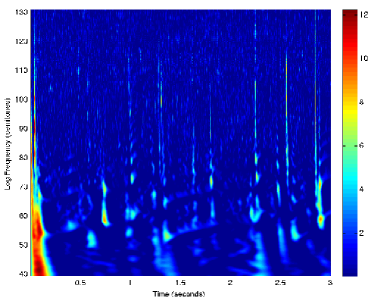
This operation is similar to edge detection in image processing and computer vision [Can86-PAMI, Lin98-IJCV] with the differences that (i) the underlying derivatives are computed in a fixed direction and that (ii) in the case of a time-causal treatment of time, the onset detection will also be associated with a temporal delay. The signed derivative operator responds to an increase in the magnitude of the signal by a positive response and to a decrease in the magnitude by a negative response. To select receptive field responses that correspond to onsets only, this operation is naturally combined with the (non-linear) logical operation: such that (see figure 11, middle right)
| (93) |
In a corresponding manner, offset detection can be performed using
| (94) |
Spectral sharpening.
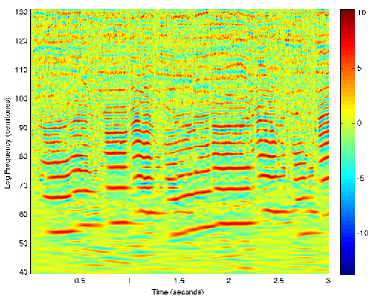
Computation of second-order Gaussian derivatives over the log-spectral domain (see figure 11, bottom left)
| (95) |
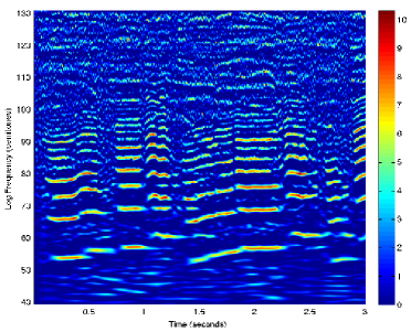
where the factor is a scale normalization factor for scale-normalized derivatives based on the Gaussian scale-space concept [Lin97-IJCV]. Depending on the value of the log-spectral scale parameter, this operation may either enhance partial tones or formants. This operation is naturally combined with the (non-linear) logical operation such that
| (96) |
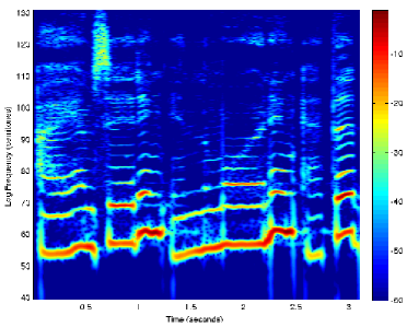
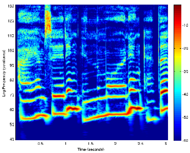
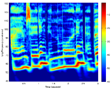
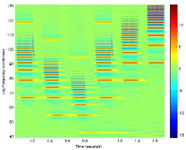
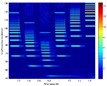
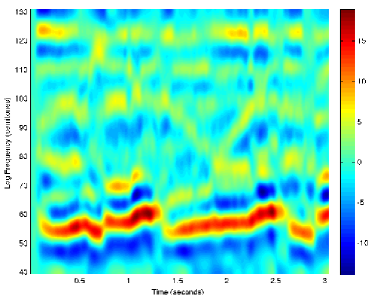
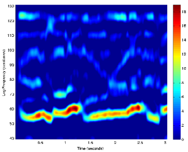
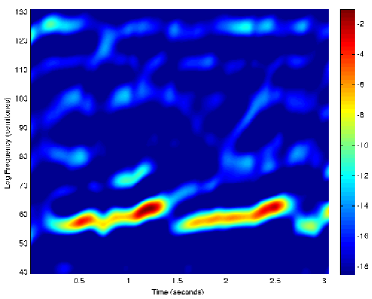
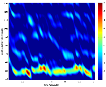
When applied at a fine log-spectral scale, this operation can be used for enhancing spectral bands corresponding to the fundamental frequency and its overtones (see figure 11, bottom right). When applied at a coarser log-spectral scale, corresponding spectral sharpening can be used for enhancing the formants of vowels (see figure 13). A similar approach involving a combination of Gaussian functions was used by [BaeMooGat93-RehabResDevel] for enhancing spectral contrast for listeners with hearing impairment and by [HecDomJouGoe11-SpeechComm] as a part of feature extraction for automatic speech recognition.
By comparing the responses to the partial tones in the second-order log-spectral derivatives to the partial tones in the raw logarithmic spectrogram, we can note that the responses to the partial tones are far more similar between different partial tones in the log-spectral derivatives compared to the raw spectrogram. This property can be understood from the invariance of spectro-temporal derivatives to local multiplications of the magnitude of a signal pointed out in section 5.1. If we model the partial tones as self-similar copies of each other at different frequencies while having different relative strength (sound pressure), then by combination of the invariance under multiplications of the magnitude in section 5.1 with the invariance of the relative bandwidth under multiplicative frequency transformations in appendix A, it follows that the spectro-temporal derivative responses to different overtones can be expected to have a similar appearance.
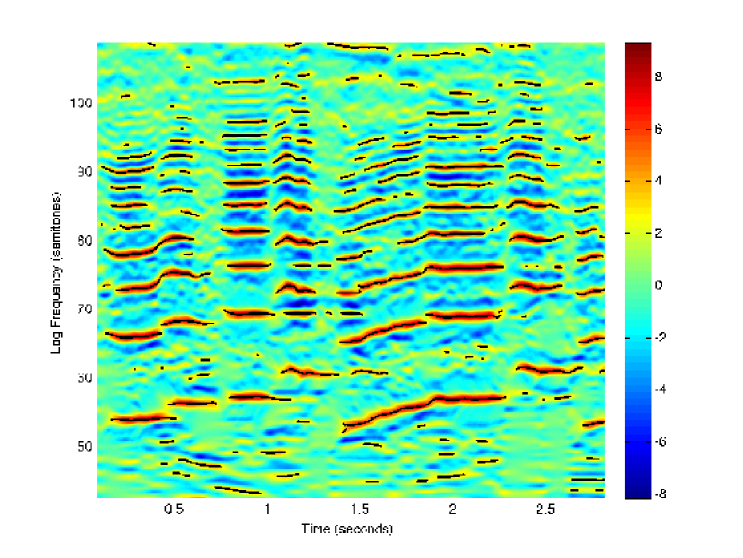
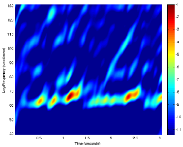
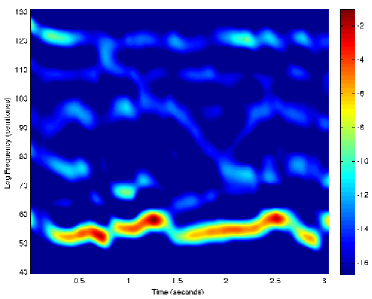
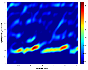
Figure 15 shows an extension of this approach, where formant enhancement is performed using glissando-adapted receptive fields, demonstrating how how formant variations for different amounts of glissando are enhanced by glissando-adapted receptive fields for corresponding values of the glissando parameter.
Capturing frequency variations over time.
Given that local spectral bands have been enhanced by second-order derivatives over logarithmic frequencies (95), we can compute local extrema over frequencies by differentiating this response
| (97) | |||
| (98) |
By interpolating for the zero-crossings of (97) that satisfy the sign constraint (98) we can obtain subresolution curves of how the frequency of partials vary over time (see figure 14).
Glissando estimation.
One way of estimating explicitly how the frequencies vary over time, is by estimating the temporal variation in the above curves, corresponding to feature tracking in the area of computer vision.
An alternative more receptive field based approach is by computing the receptive field responses for a filter bank of different glissando-receptive fields for different amounts of glissando (e.g. using second-order spectral derivatives ) analogous to the way ridge detection methods in computer vision can be expressed in terms of second-order derivatives of image intensity [Lin97-IJCV]) and then selecting the maximum response over this filter bank as the glissando estimate
| (99) |
preferably complemented by interpolation to estimate the amount of glissando by higher accuracy than the actual sampling, compare with [LapLin03-IVC, Lin13-PONE] for corresponding filter-based approaches for estimating image velocities in computer vision using a filter bank approach over different Galilean transformations.
Yet a more direct approach can be obtained by computing a spectro-temporal second-moment matrix
| (100) |
by a third layer of spectro-temporal smoothing applied to the products , and of the spectro-temporal derivatives and and then computing the glissando estimate as the value
| (101) |
that transforms the spectro-temporal moment matrix to diagonal form with the mixed being zero and corresponding to the estimation of optic flow and Galilean invariant image descriptors in the area of computer vision [LukKan81-IU, LapCapSchLin07-CVIU, Lin13-PONE]. Specifically, by computing receptive field responses using a glissando estimate according to (99) alternatively for a glissando value that corresponds to a fixed-point of (101), it can be shown that the resulting spectro-temporal receptive field responses will be invariant under glissando transformations, which would not be fully possibly based on separable spectro-temporal receptive fields only (see also [Lin13-BICY, Lin13-PONE] for analogous results regarding Galilean invariance in vision).
 |
| Time-causal model | Gaussian model |
|
 |
| Time-causal model | Gaussian model | |
|---|---|---|
|
|
 |
| Time-causal model | Gaussian model | |
|---|---|---|
|
|
 |
| Time-causal model | Gaussian model | |
|---|---|---|
|
 |
 |
|
 |
 |
| Time-causal model | Gaussian model | |
|---|---|---|
|
 |
 |
 |
| Time-causal model | Time-causal model |
 |
|
| Gaussian model | Gaussian model |
 |
|
6 Relations to biological receptive fields
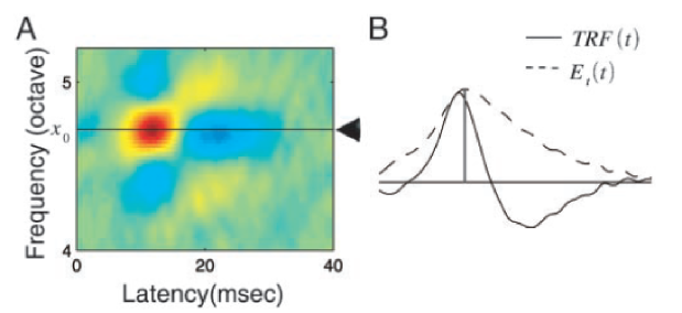
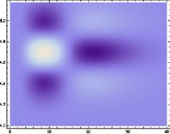
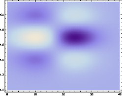
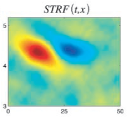
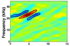
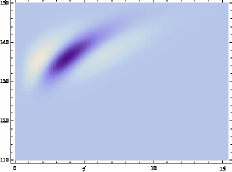
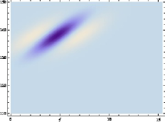
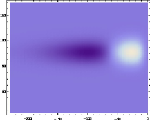
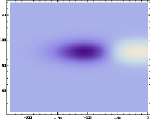
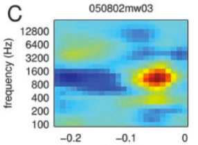
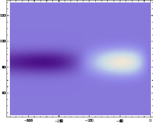
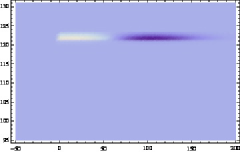
In the central nucleus of the inferior colliculus of cats, [QiuSchEsc03-JNeuroPhys] report that about 60 % of the neurons can be described as separable in the time-frequency domain (see figure 16), whereas the remaining neurons are either obliquely oriented (see figure 17) or contain multiple excitatory/inhibitory subfields. This overall structure is nicely compatible with the treatment in section 5.3, where the second-layer receptive fields are expressed in terms of spectro-temporal derivatives of either time-frequency separable spectro-temporal smoothing operations or corresponding glissando-adapted features as motivated by the structural requirements in section 5.2.
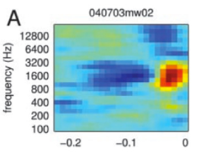
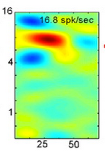
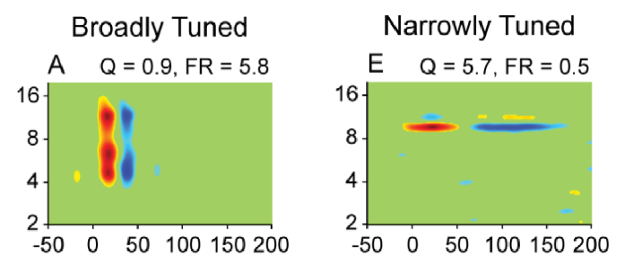
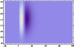
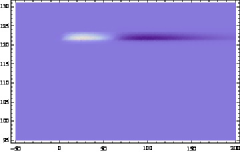
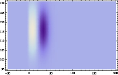
Qualitiatively similar shapes of receptive fields can also be measured from neurons in the primary auditory cortex (see figure 21 and figure 19) and for binaural receptive fields [MilEscReaSch01-JNeuroPhys]. Specifically, the use of multiple temporal and spectral scales as a main component in the theoretical model is good agreement with biological receptive fields having different degrees of spectral tuning ranging from narrow to broad (see figure 21) and different temporal extent (see figure 19). Corresponding tradeoffs between spectral and temporal tuning occur in the inferior colliculus [RodReaEsc10-JNeuroPhys]. The distribution of latencies is, however, towards somewhat shorter latencies in the thalamus than in the auditory cortex [MilEscReaSch01-JNeuroPhys], consistent with larger temporal scales in the auditory cortex than in the inferior colliculus.
Whereas spatio-temporal receptive fields estimated from neurons in the auditory cortex have been reported to reasonably well predict the neural responses for subsets of natural stimuli, [MacWehZad04-JNeuroSci] report that for many natural stimuli the responses of the auditory neurons in the primary auditory cortex cannot be predicted by the estimated linear receptive fields. [AteShaSch12-JNeuroPhys] have also reported that the dimensionality and thereby the variability of the receptive fields in the auditory cortex is significantly richer compared to the receptive fields in the inferior colliculus in the midbrain. Thus, the neurons in the primary auditory cortex appear to contain non-linearities whose functionality remains to be understood. In the inferior colliculus in the midbrain, [EscSch02-JNeuroSci] do on the other hand report that about 60 % of the receptive fields can be well described in terms of linearily integrating neurons.
In the work by [QiuSchEsc03-JNeuroPhys], the measured biological receptive fields were fitted to Gabor functions as motivated by previous use of Gabor functions for modeling visual receptive fields [Mar80-JOSA, JonPal87a, JonPal87b]. In vision, the use of Gabor functions for modelling visual receptive fields can, however, be questioned both on theoretical and empirical grounds [StoWil90-JOSA, Lin13-BICY, Lin13-PONE].444 [StoWil90-JOSA] argue that (i) only complex-valued Gabor functions that cannot describe single receptive field minimize the uncertainty relation, (ii) the real functions that minimize this relation are Gaussian derivatives rather than Gabor functions and (iii) comparisons among Gabor and alternative fits to both psychophysical and physiological data have shown that in many cases other functions (including Gaussian derivatives) provide better fits than Gabor functions do. [Lin13-BICY, Lin13-PONE] argues that in relation to invariance properties, the family of affine Gaussian kernels is closed under affine image deformations, whereas the family of Gabor functions obtained by multiplying rotationally symmetric Gaussians with sine and cosine waves is not closed under affine image deformations. This means that it is not possibly to compute truly affine invariant image representations from such Gabor functions. Instead, given a pair of images that are related by a non-uniform image deformation, the lack of affine covariance implies that there will be a systematic bias in image representations derived from such Gabor functions, corresponding to the difference between the backprojected Gabor functions in the two image domains. If using receptive profiles defined from directional derivatives of affine Gaussian kernels, it will on the other hand be possible to compute affine invariant image representations. Similar arguments about Galilean invariance hold regarding theoretical modelling of spatio-temporal receptive fields. In addition, the zero-order Gaussian receptive as well as the derivative based receptive fields can be modelled by diffusion equations, and can therefore be implemented by computations between neighbouring computational units. Specifically, biological spectro-temporal receptive fields show a marked temporal asymmetry that cannot be captured by Gabor functions for which the locations of excitatory and inhibitory subregions are uniformly spaced. Therefore, [QiuSchEsc03-JNeuroPhys] performed additional non-linear time warping to be able to fit the model to the data. Then, they modelled oblique receptive fields over the time-frequency domain using singular value decomposition to express any oblique receptive field as a sum of separable receptive fields defined from Gabor functions.
By modeling the spatio-temporal receptive fields by a combination of time-causal scale-space kernels over time and Gaussian receptive fields over logarithmic frequencies according to (90), the temporal asymmetry of the kernels constitutes an integrated part of the theory. Furthermore, oblique receptive fields in the time-frequency domain do also constitute an integrated part of the theory in terms of glissando transformations, and there is no need to decompose a glissando-receptive field as a sum of a possibly rather large number of spectro-temporal receptive fields, to be able to model the spectro-temporal receptive in a quantitiative manner. In addition, the model has been derived in a mathematically principled way from a set of structural requirements and the idealized receptive fields can be computed by a combination of diffusion equations and first-order integrators, and therefore by a biologically plausible neural architecture.
7 Relations to previous work in audio processing
Previous auditory models of human hearing have to a large extent focused on the first stages of processing including the acoustical response of the cochlea and the following neurological responses in the auditory nerve. The auditory periphery is also the stage at which it was possible to collect the first physiological and neurological data. Recently, partly due to the fast technological progress in measurement techniques, models of more high-level functions in the auditory cortex begin to emerge [MedLopFayPop10-book]. Thus the purpose has been to convert the incoming audio into a frequency-time representation in a similar way as is done in the physical-neural system in the cochlea. This is typically done in several stages taking into account both biological measurements and psychoacoustic listening test data.
The main stage is to simulate the physical resonance system in the cochlea. It is often implemented as filter bank in which the bandwidth and frequency position of each band is separated in a similar way as the cochlear nerves. A gammatone filter is often used since it has been show to be a reasonable approximation of the acoustic properties in the cochlea leading to the first neural input [PatMoo86-FreqSel, PatRobHolMcKeoZhaAll92-AudPhysPerc]. Many other types of filters have been proposed, such as the gammachirp providing better fit to non-linearities with regard to the asymmetric frequency response at loud sound pressures [IriPat97-JASA] (see also [CheHuGlaMoo11-HearRes, LopMedd01-JASA]). In a secondary stage the response of the auditory nerves arriving from the inner hair cells in the cochlea are modeled. A common version is to make a half-wave rectification, compression (square-root or logarithmic) and low-pass filtering [PatAllGig95-JASA]. In addition the local contrast can be enhanced both in time and frequency using an adaptive procedure [PatHol96-AdvSpeechHear].
Previous computational toolboxes include the auditory image model (Aim-mat) by [BleIvePat04-ActaAcust] see also [PatUnoIri03-JASA], which include all of the different parts above as well as some additional parts, and the auditory model by [Sla98-TR].
Thus, for example the auditory image model above is quite advanced and takes into account a number of biological and perceptual phenomena. However, the biological data supporting these stages seems rather scarce in particular for complex sound signals such as music. For example, the nerve responses have often been measured in animals rather than humans and with rather simple stimuli such as stationary sinusoids [Rug92-CurrOpNeuroBiol]. Many of the parts are modeled after psychoacoustic data again with simple stimuli and thus involving the whole auditory cortex and brain. A limitation is that advanced perceptual models work can be adapted to closely model a certain type of perceptual data but will typically not extrapolate to other perceptual conditions. For example, the recent loudness model by [CheHuGlaMoo11-HearRes] closely approximates perceptual data concerning several aspects of loudness but applies only to steady-state sounds. This is an indication that the formulation of the underlying model(s) is still potentially open to alternative solutions. This is not surprising giving the complexity of the task and difficulties in obtaining biological data.
The traditional auditory models are not necessarily the best choice as a front-end for modeling more high-level perceptual aspects of music and speech. These models are often very demanding in terms of computer power and memory. In addition, the resulting data may not be suitable for further processing. Therefore, in practical applications, a front-end used for analyzing perceptual phenomena is often a simplification of the complete model. Recently, alternative models have been suggested which apply general principles of auditory perception but leaving out the detailed aspects. Such a model can be a good compromise between biological/perceptual reality and computational clarity and efficiency. For example, [ChiGaoCuyMatRuSha99-JASA] used for the first stage 128 overlapping constant-Q bandpass filters with 24 filters/octave, an hair cell model with a high-pass filter, a non-linear compression, a membrane leakage low-pass filter, and a simplification of a lateral inhibitory network. In addition, they also modeled a second stage of cortical processing using spectro-temporal receptive fields (STRFs) applied on the spectrogram derived in the first stage [ChiGaoCuyMatRuSha99-JASA]. Another example of such a simplified two-stage model including an auditory spectrogram with STRFs applied to speech recognition was presented by [HecDomJouGoe11-SpeechComm].
Traditionally, the short-time Fourier transform (STFT) has been used extensively for converting the signal to a time-frequency representation, presumably due to its efficient computer implementation, the fast Fourier transform (FFT). One of the major drawbacks with the STFT is the frequency resolution, which is constant in terms of Hertz. Since the ear is approximately logarithmic with regard to the frequency band distribution, a major part of the frequency data in the upper treble region is less relevant for a perceptual analysis. Similarily the resolution in the bass range is not enough for example for determining the musical pitch using a time window that can capture the onsets of fast notes [MulEllKlaRic-SelTopSignProc].
One possibility to achieve a log-frequency spectrum is to use a bank of individual bandpass filters as discussed above and also in line with the currently proposed model. This can, however, be rather time consuming. An interesting computationally efficient compromise is therefore the constant-Q transform which uses traditional STFTs applied in a combination of downsampling and different time resolutions for different octaves [BroPuc92-JASA]. A computational toolbox was recently presented by [SchKla10-SoundMusicComp]. Using the constant-Q method, the frequency resolution will be the same across the spectrum. The time resolution will, however, vary significantly across the spectrum and still exhibit poor time resolution in the bass region.
Similar approaches using a second layer of receptive fields applied on the spectrogram have been used in particular in speech research using Gabor functions [Kle02-ActAcust, EzzBouPog07-InterSpeech, MeyKol08-InterSpeech, HecDomJouGoe11-SpeechComm, WuZhaShi11-ASLP]. For example, [HecDomJouGoe11-SpeechComm] used Gabor-based receptive fields of different orientations in the time-frequency plane of the spectrogram in combination with different transformations inspired by visual object recognition in order to capture the formant trajectories over time. The resulting features were shown to improve the performance of a speech recognition system in combination with traditional features such as mel frequency cepstral components (MFCC). In this article, we show how such and related auditory operations can be derived in principled manner.
8 Summary and discussion
We have presented a theory for how idealized models of auditory receptive fields can be formulated based on structural constraints on the first stages of auditory processing. The theory includes (i) the definition of multi-scale spectrograms at different temporal scales in such a way that a spectrogram at any coarser temporal scale can be related to a corresponding spectrogram any finer temporal scale using theoretically well-defined scale-space operations, and additionally (ii) how a second-layer of spectro-temporal receptive fields can be defined over a logarithmically transformed spectrogram in such a way that the resulting spectro-temporal receptive fields obey invariance or covariance properties under natural sound transformations including temporal shifts, variations in the sound pressure, the distance between the sound source and the observer, or a shift in the frequencies of auditory stimuli. Specifically, theoretical arguments have been presented showing how these idealized receptive fields are constrained to the presented forms from symmetry properties of the environment in combination with assumptions about the internal structure of auditory operations as motivated from requirements of handling different temporal and spectral scales in a theoretically well-founded manner.
By combining the scale-space approach with a local frequency analysis, we obtain a new way of deriving the Gabor filters as a complex-valued scale-space transform resulting from the Gaussian scale-space concept being applied to a temporal signal multiplied by a complex sine wave. We can also derive the Gamma-tone filters in a corresponding manner, as a time-causal complex scale-space transform obtained by applying a set of time-causal scale-space kernels based on first-order integrators with equal time constants coupled in cascade and applied to a temporal signal multiplied by a complex sine wave. In addition, the scale-space approach to multi-scale spectrograms leads to a new family of generalized Gamma-tone filters obtained by instead using a logarithmic distribution of the intermediate temporal scales, and which allow for different trade-offs between filter characteristics such as frequency selectivity and temporal delay.
Then, given that a multi-scale spectrogram has been defined and been transformed by taking the logarithm of the magnitude values and expressing the frequencies on a logarithmic frequency scale, to ensure natural covariance properties under variations of the sound pressure or a frequency shift in the stimulus, the theory provides a second layer of receptive fields applied to the spectrogram, based on spectro-temporal derivatives of spectro-temporal scale-space kernels. We have shown how that the derived models of idealized spectro-temporal receptive fields are uniquely determined given natural symmetry properties (scale-space axioms) and we have shown examples of how basic auditory features can be computed in this way.
Thus, the presented scale-space theory for auditory signals can be both related to existing models for auditory analysis and additionally leads to the formulation of a set of new models. Specifically, the presented theory provides a coherent framework by which auditory receptive fields at the first levels of processing in the auditory hierarchy can be expressed within the same theoretical framework. Moreover, the theory allows for provable invariance properties under temporal shifts, variations in sound pressure and logarithmic frequency shifts.
Concerning limitations of the approach, we have in the present treatment defined the second layer of receptive fields from the magnitude values of the spectrogram only, thus ignoring the local phase information. A natural extension would be to extend the formulation of the second layer of receptive fields to include the local phase of the spectrogram, which for example may provide important cues to judge if partial tones may constitute components of a harmonic spectrum belonging to the same physical source, and to formulate binaural receptive fields that are sensitive to the volumes in auditory space where a stimulus occurs.
It should also be stressed that the present approach constitutes a linear and pure feed-forward model for local receptive fields, corresponding to constant values of the filter parameters in the local diffusion equations and recurrence relations that determine the formation of the receptive fields. An interesting extension would be to adapt these filter parameters to the local input data or using top-down information, which could then provide computational mechanisms to express stimulus- and/or task-dependent receptive fields as reported by [FriShaElhKle03-NatureNeuSci, MacWehZad04-JNeuroSci, ElhFriChiSha07-JNeuroSci, Egg11-HearRes, DavFriSha12-PNAS, LauEdeHue12-PONE] and furthermore to extend the use of local receptive fields that are centered around a single frequency to multi-local operations that combine information from several distinct frequencies [PieHar05-JNeuroPhys].
In relation to such more complex non-linear mechanisms, the presented linear theory can be seen as a first principled starting point that (i) enables the computation of basic auditory features for audio processing and (ii) generates predictions about basic receptive field profiles that are qualitatively similar to biological receptive fields as measured by cell recordings in the inferior colliculus (ICC) and the primary auditory cortex (A1).
Appendix A Frequency selectivity of the spectrograms
Consider a sine wave signal with angular frequency :
| (102) |
When computing the windowed spectrogram, we multiply this signal by sine and cosine waves of different angular frequencies and integrate by a window function with temporal extent :
| (103) | |||
| (104) |
By the use of basic rules for trigonometric functions, we have
| (105) | |||
| (106) |
and the result of convolving these components with the window function can be expressed by multiplication with the Fourier transform :
| (107) | |||
| (108) |
Concerning the magnitude of the spectrogram
| (109) |
it follows that
| (110) |
If we assume that the window function should be a low-pass filter, then for close to it seems reasonable to assume that
| (111) |
Thereby, the dominant component of the spectrogram near will be given by
| (112) |
By normalizing this entity such that the maximum value at is equal to one, we can quantify the frequency selectivity for a frequency dependent window scale as
| (113) |
which on a logarithmic dB scale assumes the form
| (114) |
where we would ideally choose the temporal extent of the kernel in units of proportional to the wavelength for any angular frequency :
| (115) |
Gaussian window functions.
For a Gaussian window function we have
| (116) |
With the temporal extent of the window function proportional to the wavelength for any frequency according to (115), the frequency selectivity is given by
| (117) |
or in dB
| (118) |
Window functions defined from cascade of truncated exponential functions.
For the truncated exponential filters coupled in cascade, the Laplace transform is
| (119) |
implying that the Fourier transform is given by
| (120) |
In the special case when all the time constants are equal, we have
| (121) |
With the temporal extent of the window function proportional to the wavelength according to (115), the frequency selectivity is given by
| (122) |
or in dB
| (123) |
In the special case when all the intermediate temporal scale levels are instead distributed according to a logarithmic distribution with and according to (41) and (42), and with the temporal extent of the window function proportional to the wavelength according to (115), we obtain
| (124) |
or in dB
| (125) | |||
| (126) |
Figure 22 shows graphs of the frequency selectivity of the different types of temporal window functions for a few combinations of the underlying filter parameters. As can be seen from these graphs, the non-causal Gaussian kernel has sharper frequency selectivity compared to the time-causal kernels. Within the class of time-causal kernels, the frequency selectivity increases with the number of truncated exponential kernels that are coupled in cascade. For the logarithmic distribution of the intermediate temporal scale levels, the frequency selectivity also increases with decreasing values of the distribution parameter .
| () | (, ) | (, ) | |
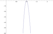 |
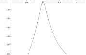 |
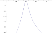 |
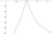 |
| () | (, ) | (, ) | |
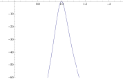 |
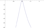 |
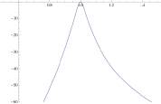 |
Dependency of the relative bandwidth on .
Notably all these expressions are functions of the ratio
| (127) |
By solving for and assuming
| (128) |
we get explicit expressions for how the relative bandwidth of the spectrogram
| (129) |
alternatively in logarithmic MIDI units
| (130) |
depends on for any , implying that the relative bandwidth increases approximately linearily with the proportionality constant , where is related to the dB level according to
| (131) |
for the Gaussian window functions and according to
| (132) |
for the time-causal kernels having a uniform distribution of the intermediate temporal scale levels. For the time-causal kernels having a logarithmic distribution of the intermediate scale levels, the parameter can be determined by solving the following equation
| (133) |
numerically given specific values of and . Table 1 shows such values for and for and as well as corresponding values for a uniform distribution of the intermediate scale levels and for a Gaussian window function.
| Relative bandwidth of temporal window functions | ||||
|---|---|---|---|---|
| -3 dB | -10 dB | -20 dB | -30 dB | |
| 0.132 | 0.242 | 0.342 | 0.418 | |
| () | 0.138 | 0.281 | 0.468 | 0.684 |
| () | 0.140 | 0.292 | 0.498 | 0.736 |
| () | 0.143 | 0.312 | 0.553 | 0.838 |
| () | 0.146 | 0.332 | 0.619 | 0.971 |
| () | 0.136 | 0.263 | 0.406 | 0.546 |
| () | 0.140 | 0.289 | 0.478 | 0.678 |
| () | 0.143 | 0.311 | 0.547 | 0.816 |
| () | 0.146 | 0.332 | 0.617 | 0.963 |
Frequency invariance.
From the invariance of the expressions (117), (122) and (124) under frequency transformations of the form
| (134) | |||
| (135) |
for any , it follows that the spectral sensitivity of the spectrogram will be independent of the angular frequency . Thereby, over the range of frequencies for which the temporal extent of the window function is proportional to the wavelength, it follows that the spectral sensitivity is invariant under a shift in frequency of the form , thus providing a foundation frequency covariant receptive fields at higher levels in the auditory hierachy.
Appendix B Temporal dynamics of the time-causal scale-space kernels
For the time-causal filters obtained by coupling truncated exponential kernels in cascade, there will be an inevitable temporal delay depending on the time constants of the individual filters.
A most straightforward way of estimating this delay is by using the additive property of mean values under convolution
| (136) |
In the special case of all the time constants being equal , this measure is given by
| (137) |
showing that the temporal increases if the temporal smoothing operation is divided into a lower number individual smoothing steps.
In the special case when the intermediate temporal scale levels are instead distributed logarithmically according to (40), with the corresponding time constants given by (41) and (42), this measure for the temporal delay does instead assume the form
| (138) |
with the limit value
| (139) |
when the number of filters tends to infinity.
By comparing equations (137), (LABEL:eq-delta-recfilt-log) and (139), we can specifically note that with increasing number of intermediate temporal scale levels, a logarithmic distribution of the intermediate scale levels implies shorter temporal delays than a uniform distribution of the intermediate scale levels.
Table 2 shows numerical values of these measures for different values of and three values of . Notably, the logarithmic distribution of the intermediate scale levels allows for significantly faster temporal dynamics than a uniform distribution.
| Temporal mean values of time-causal kernels | ||||
|---|---|---|---|---|
| () | () | () | ||
| 2 | 1.414 | 1.414 | 1.399 | 1.366 |
| 3 | 1.732 | 1.707 | 1.636 | 1.549 |
| 4 | 2.000 | 1.914 | 1.777 | 1.641 |
| 5 | 2.236 | 2.061 | 1.860 | 1.686 |
| 6 | 2.449 | 2.164 | 1.910 | 1.709 |
| 7 | 2.646 | 2.237 | 1.940 | 1.721 |
| 8 | 2.828 | 2.289 | 1.957 | 1.732 |
Additional temporal characteristics.
Because of the asymmetric tails of the time-causal temporal smoothing kernels, temporal delay estimation by the mean value may however lead to substantial overestimates compared to e.g. the position of the local maximum. To provide more precise characteristics in the case of a uniform distribution of the intermediate temporal scale levels, for which a compact closed form expression is available for the composed kernel
| (140) |
let us differentiate this function
| (141) | |||
| (142) |
and solve for the positions of the local maximum and the inflection points
| (143) | |||
| (144) | |||
| (145) |
Table 3 shows numerical values for the position of the local maximum for both types of time-causal kernels. As can be seen from the table, the temporal response properties are significantly faster for a logarithmic distribution of the intermediate scale levels compared to a uniform distribution, and the difference increases rapidly with . These temporal delay estimates are also significantly shorter than the temporal mean values, in particular for the logarithmic distribution of the intermediate scale levels.
| Temporal delays from the maxima of time-causal kernels | ||||
|---|---|---|---|---|
| () | () | () | ||
| 2 | 0.707 | 0.707 | 0.688 | 0.640 |
| 3 | 1.154 | 1.122 | 1.027 | 0.909 |
| 4 | 1.500 | 1.385 | 1.199 | 1.014 |
| 5 | 1.789 | 1.556 | 1.289 | 1.060 |
| 6 | 2.041 | 1.669 | 1.340 | 1.083 |
| 7 | 2.268 | 1.745 | 1.370 | 1.095 |
| 8 | 2.475 | 1.797 | 1.388 | 1.100 |
If we consider a temporal event that occurs as a step function over time (e.g. as an onset in the magnitude of the spectrogram which is then processed by a second layer of spectro-temporal receptive fields) and if the temporal position of this onset is estimated from a the local maximum over time in the first-order temporal derivative response, then the temporal variation in the response over time will be given by shape of the temporal smoothing kernel and the local maximum over time will occur at a time delay equal to the time at which the temporal kernel has its maximum over time. Thus, the position over time of the local maximum of the temporal smoothing kernel is highly relevant for quantifying the temporal responses characteristics of time-causal filtering operations.
Appendix C Computational implementation
The computational model for auditory receptive fields presented in this paper is based on auditory signals that are assumed to be continuous over time and with frequencies that are also assumed to take values over a continuous frequency domain. When implementing this model computationally on sampled sound signals, the continuous theory must be transferred to a discrete temporal domain where also a finite set of discrete frequencies are being used.
In this appendix we describe how the temporal and spectro-temporal receptive fields can be implemented in terms of corresponding discrete scale-space kernels that possess scale-space properties over discrete temporal and spectro-temporal domains.
C.1 Discrete temporal scale-space kernels based on recursive filters
Given a temporal signal that has been sampled for some temporal sampling density , the temporal scale in the continous model in units of seconds is first transferred to a temporal scale relative to a unit time sampling according to
| (146) |
where we have usually used sound signals with in the experiments. Then, a discrete set of intermediate temporal scale levels is defined according to (40)
| (147) |
or (44)
| (148) |
with the difference between successive scale levels according to (with )
| (149) |
For implementing the temporal smoothing operation between two such adjacent scale levels, we make use of a first-order recursive filter
| (150) |
with generating function
| (151) |
which is a time-causal kernel and can be shown to satisfy discrete scale-space properties in the sense of guaranteeing that the number of local extrema or zero-crossings in the signal will not increase [Lin90-PAMI, LF96-ECCV]. Each such filter has temporal mean value and temporal variance , and we compute from according to
| (152) |
By the additive property of variances under convolution with a positive kernel it follows that the discrete variances of the discrete temporal scale-space kernels will perfectly match those of the continuous model, whereas the mean values and the temporal delays will be somewhat different. If the temporal scale is large relative to the temporal sampling density, the discrete model can however also be seen as a good approximation in this respect.
By the time-recursive formulation of this temporal scale-space concept, it follows that the computations can be performed based on a compact temporal buffer over time which contains the temporal scale-space representations at temporal scales , and there is therefore no need for storing any additional temporal buffer of what has occured in the past to perform the corresponding temporal operations.
C.2 Discrete implementation of Gaussian smoothing
In our model, Gaussian smoothing is used both for smoothing over the spectral domain and as a non-causal model for smoothing over the temporal domain. To implement this operation on discrete sampled data, we do first (i) in the case of purely temporal smoothing transform a temporal variance in units of seconds to a temporal variance relative to a unit sampling density according to
| (153) |
or (ii) in the case of purely spectral smoothing transform a spectral smoothing scale in units of semitones to a spectral smoothing scale relative to the logspectral sampling distance and in units of variance according to
| (154) |
Then, we perform convolution with the discrete analogue of the Gaussian kernel [Lin90-PAMI]
| (155) |
where denotes the modified Bessel functions of integer order and which corresponds to the solution of the semi-discrete diffusion equation
| (156) |
where denotes the variable over the dimension of the domain, which can either be time or logarithmic frequency .
It can be shown that these kernels constitute the natural way to define a scale-space concept for discrete signals corresponding to the Gaussian scale-space over a symmetric domain in the sense of guaranteeing that the number of local extrema or zero-crossings must not increase with scale, while also ensuring a semi-group property
| (157) |
over the discrete domain which implies that representations at coarser scales can be computed from representations at finer scales using the cascade property (17).
In practice, we do based on the (exact) relation truncate the infinite discrete kernel at the tails such that
| (158) |
for some small value of of the order to . A coarse estimate of this bound can be obtained by estimating the corresponding tails of the continuous Gaussian kernel
| (159) |
using the error function and then adjusting this estimate to match (158).
For points where some part of the kernel would stretch outside the domain of available data, we mirror the data at the boundaries which has the equivalent effect of solving the diffusion equation with adiabatic boundary conditions corresponding to no heat transfer across the boundaries of the domain where data are available.
C.3 Discrete implementation of spectro-temporal receptive fields
For separable spectro-temporal receptive fields, we implement the spectro-temporal smoothing operation by separable combination of the temporal and spectral scale-space concepts in sections C.1 and C.2. From this representation, separable spectro-temporal derivative approximations are then computed from difference operators of the following types:
| (160) | |||
| (161) | |||
| (162) | |||
| (163) |
with the difference operators expressed over the appropriate dimensions, here with the implicit convention that time corresponds to the horizontal dimension in an auditory signal or a spectrogram and logarithmic frequency to the vertical (transposed) dimension.
From the general theory in [Lin93-JMIV, Lin93-Dis] it follows that computation of discrete derivative approximation in this way implies that the scale-space properties for the original zero-order signal will be transferred to the derivative approximations, thereby implying theoretically well-founded implementation of receptive fields in terms of derivatives.
For non-separable spectro-temporal receptive fields corresponding to logarithmic frequencies that vary with time by glissando , we implement the spectro-temporal smoothing operation by first warping the spectro-temporal data locally
| (164) |
using spline interpolation. Then, we apply separable spectro-temporal smoothing in the transformed domain and unwarp the result back to the original domain. Over a continuous domain, such an operation is equivalent to convolution with corresponding glissando-adapted spectro-temporal receptive fields, while being significantly faster in a discrete implementation than corresponding explicit convolution with non-separable receptive fields over two dimensions.
In addition to a transfer of the scale-space properties from the continuous model to the discrete implementation, all the components in this discretization, the discrete Gaussian kernel, the time-recursive filters and the discrete derivative approximations, can be seen as mathematical approximations of the corresponding continuous counterparts.T Thereby, if follows that the behaviour of the discrete implementation will approach the behaviour of the corresponding continuous model as the temporal sampling rate and the sampling rate in the logarithmic frequency domain increase. Choosing appropriate sampling rates in an actual implementation is a trade-off between computational accuracy and computational efficiency.
References
- [1] \harvarditemAertsen \harvardand Johannesma1981AerJoh81-BICY Aertsen, A. M. H. J. \harvardand Johannesma, P. I. M. \harvardyearleft1981\harvardyearright, ‘The spectro-temporal receptive field: A functional characterization of auditory neurons’, Biological Cybernetics 42(2), 133–143.
- [2] \harvarditem[Ambikairajah et al.]Ambikairajah, Epps \harvardand Lin2001AmbEppLin01-ICASSP Ambikairajah, E., Epps, J. \harvardand Lin, L. \harvardyearleft2001\harvardyearright, Wideband speech and audio coding using gammatone filter banks, in ‘IEEE International Conference on Acoustics, Speech, and Signal Processing (ICASSP’01)’, Vol. 2, pp. 773–776.
- [3] \harvarditem[Andoni et al.]Andoni, Li \harvardand Pollack2007AndLiPol07-JNeuroSci Andoni, S., Li, N. \harvardand Pollack, G. D. \harvardyearleft2007\harvardyearright, ‘Spectrotemporal receptive fields in the inferior colliculus revealing selectivity for spectral motion in conspecific vocalizations’, Journal of Neuroscience 27(18), 4882–4893.
- [4] \harvarditemAtencio \harvardand Schreiner2012AteSch12-PONE Atencio, C. A. \harvardand Schreiner, C. E. \harvardyearleft2012\harvardyearright, ‘Spectrotemporal processing in spectral tuning modules of cat primary auditory cortex’, PLOS ONE 7(2), e31537.
- [5] \harvarditem[Atencio et al.]Atencio, Sharpee \harvardand Schreiner2012AteShaSch12-JNeuroPhys Atencio, C. A., Sharpee, T. O. \harvardand Schreiner, C. E. \harvardyearleft2012\harvardyearright, ‘Receptive field dimensionality increases from the auditory midbrain to cortex’, Journal of Neurophysiology 107(10), 2594–2603.
- [6] \harvarditem[Baer et al.]Baer, Moore \harvardand Gatehouse1993BaeMooGat93-RehabResDevel Baer, T., Moore, B. C. J. \harvardand Gatehouse, S. \harvardyearleft1993\harvardyearright, ‘Spectral contrast enhancement of speech in noise for listeners with sensorineural hearing impairment: Effects on intelligibility, quality, and response times’, Journal of Rehabilitation Research and Development 30, 49–49.
- [7] \harvarditem[Bleeck et al.]Bleeck, Ives \harvardand Patterson2004BleIvePat04-ActaAcust Bleeck, S., Ives, T. \harvardand Patterson, R. D. \harvardyearleft2004\harvardyearright, ‘Aim-mat: the auditory image model in MATLAB’, Acta Acustica United with Acustica 90(4), 781–787.
- [8] \harvarditemBrown \harvardand Puckette1992BroPuc92-JASA Brown, J. C. \harvardand Puckette, M. S. \harvardyearleft1992\harvardyearright, ‘An efficient algorithm for the calculation of a constant Q transform’, The Journal of the Acoustical Society of America 92(5), 2698–2701.
- [9] \harvarditemCanny1986Can86-PAMI Canny, J. \harvardyearleft1986\harvardyearright, ‘A computational approach to edge detection’, IEEE Trans. Pattern Analysis and Machine Intell. 8(6), 679–698.
- [10] \harvarditem[Chen et al.]Chen, Hu, Glasberg \harvardand Moore2011CheHuGlaMoo11-HearRes Chen, Z., Hu, G., Glasberg, B. R. \harvardand Moore, B. C. J. \harvardyearleft2011\harvardyearright, ‘A new method of calculating auditory excitation patterns and loudness for steady sounds’, Hearing Research 282(1), 204–215.
- [11] \harvarditem[Chi et al.]Chi, Gao, Guyton, Ru \harvardand Shamma1999ChiGaoCuyMatRuSha99-JASA Chi, T., Gao, Y., Guyton, M. C., Ru, P. \harvardand Shamma, S. \harvardyearleft1999\harvardyearright, ‘Spectro-temporal modulation transfer functions and speech intelligibility’, The Journal of the Acoustical Society of America 106(5), 2719–2732.
- [12] \harvarditemConway \harvardand Livingstone2006ConLiv06-JNeurSci Conway, B. R. \harvardand Livingstone, M. S. \harvardyearleft2006\harvardyearright, ‘Spatial and temporal properties of cone signals in alert macaque primary visual cortex’, Journal of Neuroscience 26(42), 10826–10846.
- [13] \harvarditem[David et al.]David, Fritz \harvardand Shamma2012DavFriSha12-PNAS David, S. V., Fritz, J. B. \harvardand Shamma, S. A. \harvardyearleft2012\harvardyearright, ‘Task reward structure shapes rapid receptive field plasticity in auditory cortex’, Proceedings of the National Academy of Sciences 109(6), 2144–2149.
- [14] \harvarditemDeAngelis \harvardand Anzai2004deAngAnz04-VisNeuroSci DeAngelis, G. C. \harvardand Anzai, A. \harvardyearleft2004\harvardyearright, A modern view of the classical receptive field: Linear and non-linear spatio-temporal processing by V1 neurons, in L. M. Chalupa \harvardand J. S. Werner, eds, ‘The Visual Neurosciences’, Vol. 1, MIT Press, pp. 704–719.
- [15] \harvarditem[DeAngelis et al.]DeAngelis, Ohzawa \harvardand Freeman1995DeAngOhzFre95-TINS DeAngelis, G. C., Ohzawa, I. \harvardand Freeman, R. D. \harvardyearleft1995\harvardyearright, ‘Receptive field dynamics in the central visual pathways’, Trends in Neuroscience 18(10), 451–457.
- [16] \harvarditem[Domont et al.]Domont, Heckmann, Joublin \harvardand Goerick2008DomHecJouGoe08-ICASSP Domont, X., Heckmann, M., Joublin, F. \harvardand Goerick, C. \harvardyearleft2008\harvardyearright, Hierarchical spectro-temporal features for robust speech recognition, in ‘International Conference on Acoustics, Speech and Signal Processing (ICASSP’08)’, pp. 4417–4420.
- [17] \harvarditemEggermont2011Egg11-HearRes Eggermont, J. J. \harvardyearleft2011\harvardyearright, ‘Context dependence of spectro-temporal receptive fields with implications for neural coding’, Hearing Research 271(1–2), 123–132.
- [18] \harvarditem[Elhilali et al.]Elhilali, Fritz, Chi \harvardand Shamma2007ElhFriChiSha07-JNeuroSci Elhilali, M., Fritz, J., Chi, T.-S. \harvardand Shamma, S. \harvardyearleft2007\harvardyearright, ‘Auditory cortical receptive fields: Stable entities with plastic abilities’, The Journal of Neuroscience 27(39), 10372–10382.
- [19] \harvarditemEscabi \harvardand Schreiner2002EscSch02-JNeuroSci Escabi, M. A. \harvardand Schreiner, C. E. \harvardyearleft2002\harvardyearright, ‘Nonlinear spectrotemporal sound analysis by neurons in the auditory midbrain’, The Journal of Neuroscience 22(10), 4114–4131.
- [20] \harvarditem[Ezzat et al.]Ezzat, Bouvrie \harvardand Poggio2007EzzBouPog07-InterSpeech Ezzat, T., Bouvrie, J. V. \harvardand Poggio, T. \harvardyearleft2007\harvardyearright, Spectro-temporal analysis of speech using 2-D Gabor filters, in ‘INTERSPEECH’, pp. 506–509.
- [21] \harvarditemFletcher1934Fle34-JASA Fletcher, H. \harvardyearleft1934\harvardyearright, ‘Loudness, pitch and the timbre of musical tones and their relation to the intensity, the frequency and the overtone structure’, Journal of the Acoustical Society of America .
- [22] \harvarditemFlorack1997Flo97-book Florack, L. M. J. \harvardyearleft1997\harvardyearright, Image Structure, Series in Mathematical Imaging and Vision, Springer.
- [23] \harvarditem[Fritz et al.]Fritz, Shamma, Elhilali \harvardand Klein2003FriShaElhKle03-NatureNeuSci Fritz, J., Shamma, S., Elhilali, M. \harvardand Klein, D. \harvardyearleft2003\harvardyearright, ‘Rapid task-related plasticity of spectro-temporal receptive fields in primary auditory cortex’, Nature Neuroscience 6(11), 1216–1223.
- [24] \harvarditemGabor1946Gab46 Gabor, D. \harvardyearleft1946\harvardyearright, ‘Theory of communication’, J. of the IEE 93, 429–457.
- [25] \harvarditemGreenwood1990Gre90-JASA Greenwood, D. D. \harvardyearleft1990\harvardyearright, ‘A cochlear frequency-position function for several species — 29 years later’, The Journal of the Acoustical Society of America 87(6), 2592–2605.
- [26] \harvarditemHartmann1996Har96-JASA Hartmann, W. M. \harvardyearleft1996\harvardyearright, ‘Pitch, periodicity, and auditory organization’, The Journal of the Acoustical Society of America 100(6), 3491–3502.
- [27] \harvarditem[Hartmann et al.]Hartmann, McAdams \harvardand Smith1990HarMcAdaSmi90-JASA Hartmann, W. M., McAdams, S. \harvardand Smith, B. K. \harvardyearleft1990\harvardyearright, ‘Hearing a mistuned harmonic in an otherwise periodic complex tone’, The Journal of the Acoustical Society of America 88(4), 1712–1724.
- [28] \harvarditem[He et al.]He, Lech, Maddage \harvardand Allen2009HeLecMadAll09-AffComp He, L., Lech, M., Maddage, N. \harvardand Allen, N. \harvardyearleft2009\harvardyearright, Stress and emotion recognition using log-Gabor filter analysis of speech spectrograms, in ‘Affective Computing and Intelligent Interaction and Workshops (ACII ’09)’, pp. 1–6.
- [29] \harvarditem[Heckmann et al.]Heckmann, Domont, Joublin \harvardand Goerick2011HecDomJouGoe11-SpeechComm Heckmann, M., Domont, X., Joublin, F. \harvardand Goerick, C. \harvardyearleft2011\harvardyearright, ‘A hierarchical framework for spectro-temporal feature extraction’, Speech Communication 53(5), 736–752.
- [30] \harvarditemHewitt \harvardand Meddis1994HewMed94-JASA Hewitt, M. J. \harvardand Meddis, R. \harvardyearleft1994\harvardyearright, ‘A computer model of amplitude-modulation sensitivity of single units in the inferior colliculus’, The Journal of the Acoustical Society of America 95(4), 2145–2159.
- [31] \harvarditemHirschmann \harvardand Widder1955HirWid55 Hirschmann, I. I. \harvardand Widder, D. V. \harvardyearleft1955\harvardyearright, The Convolution Transform, Princeton University Press, Princeton, New Jersey.
- [32] \harvarditemHohmann2002Hoh02-GammaTone Hohmann, V. \harvardyearleft2002\harvardyearright, ‘Frequency analysis and synthesis using a Gammatone filterbank’, Acta Acustica United with Acustica 88(3), 433–442.
- [33] \harvarditemHubel \harvardand Wiesel1959HubWie59-Phys Hubel, D. H. \harvardand Wiesel, T. N. \harvardyearleft1959\harvardyearright, ‘Receptive fields of single neurones in the cat’s striate cortex’, J Physiol 147, 226–238.
- [34] \harvarditemHubel \harvardand Wiesel1962HubWie62-Phys Hubel, D. H. \harvardand Wiesel, T. N. \harvardyearleft1962\harvardyearright, ‘Receptive fields, binocular interaction and functional architecture in the cat’s visual cortex’, J Physiol 160, 106–154.
- [35] \harvarditemIijima1962Iij62 Iijima, T. \harvardyearleft1962\harvardyearright, Observation theory of two-dimensional visual patterns, Technical report, Papers of Technical Group on Automata and Automatic Control, IECE, Japan.
- [36] \harvarditemIrino \harvardand Patterson1997IriPat97-JASA Irino, T. \harvardand Patterson, R. D. \harvardyearleft1997\harvardyearright, ‘A time-domain, level-dependent auditory filter: The gammachirp’, The Journal of the Acoustical Society of America 101(1), 412–419.
- [37] \harvarditemJohannesma1972Joh72-HearTheory Johannesma, P. I. M. \harvardyearleft1972\harvardyearright, The pre-response stimulus ensemble of neurons in the cochlear nucleus, in ‘IPO Symposium on Hearing Theory’, Eindhoven, The Netherlands, pp. 58–69.
- [38] \harvarditemJohnson1980Joh80-JASA Johnson, D. H. \harvardyearleft1980\harvardyearright, ‘The relationship between spike rate and synchrony in responses of auditory-nerve fibers to single tones’, The Journal of the Acoustical Society of America 68(4), 1115–1122.
- [39] \harvarditemJones \harvardand Palmer1987aJonPal87b Jones, J. \harvardand Palmer, L. \harvardyearleft1987a\harvardyearright, ‘An evaluation of the two-dimensional Gabor filter model of simple receptive fields in cat striate cortex’, J. of Neurophysiology 58, 1233–1258.
- [40] \harvarditemJones \harvardand Palmer1987bJonPal87a Jones, J. \harvardand Palmer, L. \harvardyearleft1987b\harvardyearright, ‘The two-dimensional spatial structure of simple receptive fields in cat striate cortex’, J. of Neurophysiology 58, 1187–1211.
- [41] \harvarditem[Kandel et al.]Kandel, Schwartz \harvardand Jessel2000KanSchJes00-PrincNeurSci Kandel, E. R., Schwartz, J. H. \harvardand Jessel, T. M. \harvardyearleft2000\harvardyearright, Principles of Neural Science, 4th edition edn, McGraw-Hill.
- [42] \harvarditemKleinschmidt2002Kle02-ActAcust Kleinschmidt, M. \harvardyearleft2002\harvardyearright, ‘Methods for capturing spectro-temporal modulations in automatic speech recognition’, Acta Acustica united with Acustica 88(3), 416–422.
- [43] \harvarditemKleinschmidt \harvardand Gelbart2002KleGel02-InterSpeech Kleinschmidt, M. \harvardand Gelbart, D. \harvardyearleft2002\harvardyearright, Improving word accuracy with Gabor feature extraction, in ‘INTERSPEECH’.
- [44] \harvarditemKoch1999Koch99-book Koch, C. \harvardyearleft1999\harvardyearright, Biophysics of Computation: Information Processing in Single Neurons, Oxford University Press.
- [45] \harvarditemKoenderink1984Koe84 Koenderink, J. J. \harvardyearleft1984\harvardyearright, ‘The structure of images’, Biological Cybernetics 50, 363–370.
- [46] \harvarditemKoenderink1988Koe88-BC Koenderink, J. J. \harvardyearleft1988\harvardyearright, ‘Scale-time’, Biological Cybernetics 58, 159–162.
- [47] \harvarditemKoenderink \harvardand van Doorn1992KoeDoo92-PAMI Koenderink, J. J. \harvardand van Doorn, A. J. \harvardyearleft1992\harvardyearright, ‘Generic neighborhood operators’, IEEE Trans. Pattern Analysis and Machine Intell. 14(6), 597–605.
- [48] \harvarditem[Laptev et al.]Laptev, Caputo, Schuldt \harvardand Lindeberg2007LapCapSchLin07-CVIU Laptev, I., Caputo, B., Schuldt, C. \harvardand Lindeberg, T. \harvardyearleft2007\harvardyearright, ‘Local velocity-adapted motion events for spatio-temporal recognition’, Computer Vision and Image Understanding 108, 207–229.
- [49] \harvarditemLaptev \harvardand Lindeberg2004LapLin03-IVC Laptev, I. \harvardand Lindeberg, T. \harvardyearleft2004\harvardyearright, ‘Velocity-adapted spatio-temporal receptive fields for direct recognition of activities’, Image and Vision Computing 22(2), 105–116.
- [50] \harvarditem[Laudanski et al.]Laudanski, Edeline \harvardand Huetz2012LauEdeHue12-PONE Laudanski, J., Edeline, J.-M. \harvardand Huetz, C. \harvardyearleft2012\harvardyearright, ‘Differences between spectro-temporal receptive fields derived from artificial and natural stimuli in the auditory cortex’, PLOS ONE 7(11), e50539.
- [51] \harvarditemLindeberg1990Lin90-PAMI Lindeberg, T. \harvardyearleft1990\harvardyearright, ‘Scale-space for discrete signals’, IEEE Trans. Pattern Analysis and Machine Intell. 12(3), 234–254.
- [52] \harvarditemLindeberg1993aLin93-JMIV Lindeberg, T. \harvardyearleft1993a\harvardyearright, ‘Discrete derivative approximations with scale-space properties: A basis for low-level feature extraction’, J. of Mathematical Imaging and Vision 3(4), 349–376.
- [53] \harvarditemLindeberg1993bLin92-PAMI Lindeberg, T. \harvardyearleft1993b\harvardyearright, ‘Effective scale: A natural unit for measuring scale-space lifetime’, IEEE Trans. Pattern Analysis and Machine Intell. 15(10), 1068–1074.
- [54] \harvarditemLindeberg1994aLin94-SI Lindeberg, T. \harvardyearleft1994a\harvardyearright, ‘Scale-space theory: A basic tool for analysing structures at different scales’, Journal of Applied Statistics 21(2), 225–270. Also available from http://www.csc.kth.se/tony/abstracts/Lin94-SI-abstract.html.
- [55] \harvarditemLindeberg1994bLin93-Dis Lindeberg, T. \harvardyearleft1994b\harvardyearright, Scale-Space Theory in Computer Vision, The Springer International Series in Engineering and Computer Science, Springer.
- [56] \harvarditemLindeberg1996Lin96-ScSp Lindeberg, T. \harvardyearleft1996\harvardyearright, On the axiomatic foundations of linear scale-space, in J. Sporring, M. Nielsen, L. Florack \harvardand P. Johansen, eds, ‘Gaussian Scale-Space Theory: Proc. PhD School on Scale-Space Theory’, Springer, Copenhagen, Denmark.
- [57] \harvarditemLindeberg1998aLin98-IJCV Lindeberg, T. \harvardyearleft1998a\harvardyearright, ‘Edge detection and ridge detection with automatic scale selection’, Int. J. of Computer Vision 30(2), 117–154.
- [58] \harvarditemLindeberg1998bLin97-IJCV Lindeberg, T. \harvardyearleft1998b\harvardyearright, ‘Feature detection with automatic scale selection’, Int. J. of Computer Vision 30(2), 77–116.
- [59] \harvarditemLindeberg2008Lin08-EncCompSci Lindeberg, T. \harvardyearleft2008\harvardyearright, Scale-space, in B. Wah, ed., ‘Encyclopedia of Computer Science and Engineering’, John Wiley and Sons, Hoboken, New Jersey, pp. 2495–2504.
- [60] \harvarditemLindeberg2011Lin10-JMIV Lindeberg, T. \harvardyearleft2011\harvardyearright, ‘Generalized Gaussian scale-space axiomatics comprising linear scale-space, affine scale-space and spatio-temporal scale-space’, J. of Mathematical Imaging and Vision 40(1), 36–81.
- [61] \harvarditemLindeberg2013aLin13-BICY Lindeberg, T. \harvardyearleft2013a\harvardyearright, ‘A computational theory of visual receptive fields’, Biological Cybernetics 107(6), 589–635.
- [62] \harvarditemLindeberg2013bLin13-PONE Lindeberg, T. \harvardyearleft2013b\harvardyearright, ‘Invariance of visual operations at the level of receptive fields’, PLOS ONE 8(7), e66990.
- [63] \harvarditemLindeberg \harvardand Bretzner2003LinBre03-ScSp Lindeberg, T. \harvardand Bretzner, L. \harvardyearleft2003\harvardyearright, Real-time scale selection in hybrid multi-scale representations, in L. Griffin \harvardand M. Lillholm, eds, ‘Proc. Scale-Space Methods in Computer Vision: Scale-Space’03’, Vol. 2695 of Lecture Notes in Computer Science, Springer, Isle of Skye, Scotland, pp. 148–163.
- [64] \harvarditemLindeberg \harvardand Fagerström1996LF96-ECCV Lindeberg, T. \harvardand Fagerström, D. \harvardyearleft1996\harvardyearright, Scale-space with causal time direction, in ‘Proc. ECCV’96’, Vol. 1064, Springer, Cambridge, UK, pp. 229–240.
- [65] \harvarditemLobo \harvardand Loizou2003LobLoi03-ICASSP Lobo, A. P. \harvardand Loizou, P. \harvardyearleft2003\harvardyearright, Voiced/unvoiced speech discrimination in noise using Gabor atomic decomposition, in ‘Proc. Acoustics, Speech, and Signal Processing (ICASSP’03)’, Vol. 1, pp. 820–823.
- [66] \harvarditemLopez-Poveda \harvardand Meddis2001LopMedd01-JASA Lopez-Poveda, E. A. \harvardand Meddis, R. \harvardyearleft2001\harvardyearright, ‘A human nonlinear cochlear filterbank’, The Journal of the Acoustical Society of America 110(6), 3107–3118.
- [67] \harvarditemLukas \harvardand Kanade1981LukKan81-IU Lukas, B. D. \harvardand Kanade, T. \harvardyearleft1981\harvardyearright, An iterative image registration technique with an application to stereo vision, in ‘Image Understanding Workshop’.
- [68] \harvarditem[Machens et al.]Machens, Wehr \harvardand Zador2004MacWehZad04-JNeuroSci Machens, C. K., Wehr, M. S. \harvardand Zador, A. M. \harvardyearleft2004\harvardyearright, ‘Linearity of cortical receptive fields measures with natural sounds’, The Journal of Neuroscience 24(5), 1089–1100.
- [69] \harvarditemMarcelja1980Mar80-JOSA Marcelja, S. \harvardyearleft1980\harvardyearright, ‘Mathematical description of the responses of simple cortical cells’, J. of the Optical Society of America 70(11), 1297–1300.
- [70] \harvarditem[Meddis et al.]Meddis, Lopez-Poveda, Fay \harvardand Popper2010MedLopFayPop10-book Meddis, R., Lopez-Poveda, E., Fay, R. R. \harvardand Popper, A. N. \harvardyearleft2010\harvardyearright, Computational models of the auditory system, Vol. 35, Springer.
- [71] \harvarditemMeyer \harvardand Kollmeier2008MeyKol08-InterSpeech Meyer, B. T. \harvardand Kollmeier, B. \harvardyearleft2008\harvardyearright, Optimization and evaluation of Gabor feature sets for ASR, in ‘INTERSPEECH’, pp. 906–909.
- [72] \harvarditem[Miller et al.]Miller, Escabi, Read \harvardand Schreiner2001MilEscReaSch01-JNeuroPhys Miller, L. M., Escabi, N. A., Read, H. L. \harvardand Schreiner, C. \harvardyearleft2001\harvardyearright, ‘Spectrotemporal receptive fields in the lemniscal auditory thalamus and cortex’, Journal of Neurophysiology 87(1), 516–527.
- [73] \harvarditemMoore1973Moo73-JASA Moore, B. C. J. \harvardyearleft1973\harvardyearright, ‘Frequency difference limens for short-duration tones’, The Journal of the Acoustical Society of America 54(3), 610–619.
- [74] \harvarditem[Muller et al.]Muller, Ellis, Klapuri \harvardand Richard2011MulEllKlaRic-SelTopSignProc Muller, M., Ellis, D. P. W., Klapuri, A. \harvardand Richard, G. \harvardyearleft2011\harvardyearright, ‘Signal processing for music analysis’, IEEE Journal of Selected Topics in Signal Processing 5(6), 1088–1110.
- [75] \harvarditem[Ngamkham et al.]Ngamkham, Sawigun, Hiseni \harvardand Serdijn2010NgaSawHisSer10-ISCAS Ngamkham, W., Sawigun, C., Hiseni, S. \harvardand Serdijn, W. A. \harvardyearleft2010\harvardyearright, Analog complex gammatone filter for cochlear implant channels, in ‘Proceedings of 2010 IEEE International Symposium on Circuits and Systems (ISCAS)’, pp. 969–972.
- [76] \harvarditemPalmer1999Pal99-Book Palmer, S. E. \harvardyearleft1999\harvardyearright, Vision Science: Photons to Phenomenology, MIT Press. First Edition.
- [77] \harvarditem[Patterson et al.]Patterson, Allerhand \harvardand Giguere1995PatAllGig95-JASA Patterson, R. D., Allerhand, M. H. \harvardand Giguere, C. \harvardyearleft1995\harvardyearright, ‘Time-domain modeling of peripheral auditory processing: A modular architecture and a software platform’, The Journal of the Acoustical Society of America 98(4), 1890–1894.
- [78] \harvarditemPatterson \harvardand Holdsworth1996PatHol96-AdvSpeechHear Patterson, R. D. \harvardand Holdsworth, J. \harvardyearleft1996\harvardyearright, ‘A functional model of neural activity patterns and auditory images’, Advances in Speech, Hearing and Language Processing 3(Part B), 547–563.
- [79] \harvarditemPatterson \harvardand Moore1986PatMoo86-FreqSel Patterson, R. D. \harvardand Moore, B. C. J. \harvardyearleft1986\harvardyearright, Auditory filters and excitation patterns as representations of frequency resolution, in B. C. J. Moore, ed., ‘Frequency selectivity in hearing’, Academic Press, pp. 123–177.
- [80] \harvarditem[Patterson et al.]Patterson, Nimmo-Smith, Holdsworth \harvardand Rice1987PatNimHolRic87-GammaTone Patterson, R. D., Nimmo-Smith, I., Holdsworth, J. \harvardand Rice, P. \harvardyearleft1987\harvardyearright, An efficient auditory filterbank based on the gammatone function, in ‘A meeting of the IOC Speech Group on Auditory Modelling at RSRE’, Vol. 2:7.
- [81] \harvarditem[Patterson et al.]Patterson, Robinson, Holdsworth, McKeown, Zhang \harvardand Allerhand1992PatRobHolMcKeoZhaAll92-AudPhysPerc Patterson, R. D., Robinson, K., Holdsworth, J., McKeown, D., Zhang, C. \harvardand Allerhand, M. \harvardyearleft1992\harvardyearright, ‘Complex sounds and auditory images’, Auditory Physiology and Perception 83, 429–446.
- [82] \harvarditem[Patterson et al.]Patterson, Unoki \harvardand Irino2003PatUnoIri03-JASA Patterson, R. D., Unoki, M. \harvardand Irino, T. \harvardyearleft2003\harvardyearright, ‘Extending the domain of center frequencies for the compressive gammachirp auditory filter’, The Journal of the Acoustical Society of America 114(3), 1529–1542.
- [83] \harvarditemPienkowski \harvardand Harrison2005PieHar05-JNeuroPhys Pienkowski, M. \harvardand Harrison, R. V. \harvardyearleft2005\harvardyearright, ‘Tone frequency maps and receptive fields in the developing chincilla auditory cortex’, Journal of Neurophysiology 93(1), 454–466.
- [84] \harvarditem[Qiu et al.]Qiu, Schreiner \harvardand Escabi2003QiuSchEsc03-JNeuroPhys Qiu, A., Schreiner, C. E. \harvardand Escabi, M. A. \harvardyearleft2003\harvardyearright, ‘Gabor analysis of auditory midbrain receptive fields: Spectro-temporal and binaural composition’, Journal of Neurophysiology 90(1), 456–476.
- [85] \harvarditem[Rodriguez et al.]Rodriguez, Read \harvardand Escabi2010RodReaEsc10-JNeuroPhys Rodriguez, F. A., Read, H. L. \harvardand Escabi, M. A. \harvardyearleft2010\harvardyearright, ‘Spectral and temporal modulation tradeoff in the inferior colliculus’, Journal of Neurophysiology 103(2), 887–903.
- [86] \harvarditem[Romani et al.]Romani, Williamson \harvardand Kaufman1982RomWilKau82-Science Romani, G. L., Williamson, S. J. \harvardand Kaufman, L. \harvardyearleft1982\harvardyearright, ‘Tonotopic organization of the human auditory cortex’, Science 216(4552), 1339–1340.
- [87] \harvarditemRuggero1992Rug92-CurrOpNeuroBiol Ruggero, M. A. \harvardyearleft1992\harvardyearright, ‘Responses to sound of the basilar membrane of the mammalian cochlea’, Current Opinion in Neurobiology 2(4), 449–456.
- [88] \harvarditemSameh \harvardand Lachiri2013SamLac12-SpeechTech Sameh, S. \harvardand Lachiri, Z. \harvardyearleft2013\harvardyearright, ‘Multiclass support vector machines for environmental sounds classification in visual domain based on log-Gabor filters’, International Journal of Speech Technology 16(2), 203–213.
- [89] \harvarditem[Schädler et al.]Schädler, Meyer \harvardand Kollmeier2012SchMeyKol12-JASA Schädler, M. R., Meyer, B. T. \harvardand Kollmeier, B. \harvardyearleft2012\harvardyearright, ‘Spectro-temporal modulation subspace-spanning filter bank features for robust automatic speech recognition’, The Journal of the Acoustical Society of America 131(5), 4134–4151.
- [90] \harvarditem[Schlute et al.]Schlute, Bezrukov, Wagner \harvardand Ney2007SchBezWagNey07-ICASSP Schlute, R., Bezrukov, L., Wagner, H. \harvardand Ney, H. \harvardyearleft2007\harvardyearright, Gammatone features and feature combination for large vocabulary speech recognition, in ‘IEEE International Conference on Acoustics, Speech and Signal Processing (ICASSP’07)’, Vol. IV, pp. 649–652.
- [91] \harvarditemSchörkhuber \harvardand Klapuri2010SchKla10-SoundMusicComp Schörkhuber, C. \harvardand Klapuri, A. \harvardyearleft2010\harvardyearright, Constant-Q transform toolbox for music processing, in ‘7th Sound and Music Computing Conference’, Barcelona, Spain, pp. 3–64.
- [92] \harvarditemSlaney1998Sla98-TR Slaney, M. \harvardyearleft1998\harvardyearright, ‘Auditory toolbox’, Interval Research Corporation, Tech. Rep. 10.
- [93] \harvarditem[Sporring et al.]Sporring, Nielsen, Florack \harvardand Johansen1996SpoNieFloJoh96-SCSPTH Sporring, J., Nielsen, M., Florack, L. \harvardand Johansen, P., eds \harvardyearleft1996\harvardyearright, Gaussian Scale-Space Theory: Proc. PhD School on Scale-Space Theory, Series in Mathematical Imaging and Vision, Springer, Copenhagen, Denmark.
- [94] \harvarditemStork \harvardand Wilson1990StoWil90-JOSA Stork, D. G. \harvardand Wilson, H. R. \harvardyearleft1990\harvardyearright, ‘Do Gabor functions provide appropriate descriptions of visual cortical receptive fields’, J. of the Optical Society of America 7(8), 1362–1373.
- [95] \harvarditemter Haar Romeny2003Haa04-book ter Haar Romeny, B. \harvardyearleft2003\harvardyearright, Front-End Vision and Multi-Scale Image Analysis, Springer.
- [96] \harvarditem[Theunissen et al.]Theunissen, Sen \harvardand Doupe2000TheSenDou-JNeuroSci Theunissen, F. E., Sen, K. \harvardand Doupe, A. J. \harvardyearleft2000\harvardyearright, ‘Spectro-temporal receptive fields of nonlinearu auditory neurons obtained using natural sounds’, The Journal of Neuroscience 20(6), 2315–2331.
- [97] \harvarditemvan de Boogart \harvardand Lienhart2006BooLie06-ICASSP van de Boogart, C. G. \harvardand Lienhart, R. \harvardyearleft2006\harvardyearright, Fast Gabor transformation for processing high quality audio, in ‘Proc. Acoustics, Speech and Signal Processing (ICASSP’06)’, Vol. III, pp. 161–164.
- [98] \harvarditemvan Immerseel \harvardand Peeters2003ImmPee03-AcResLettOnLine van Immerseel, L. \harvardand Peeters, S. \harvardyearleft2003\harvardyearright, ‘Digital implementation of linear Gammatone filters: Comparison of design methods’, Acoustics Research Letters Online 4(3), 59–64.
- [99] \harvarditem[Weickert et al.]Weickert, Ishikawa \harvardand Imiya1999WeiIshImi99-JMIV Weickert, J., Ishikawa, S. \harvardand Imiya, A. \harvardyearleft1999\harvardyearright, ‘Linear scale-space has first been proposed in Japan’, J. of Mathematical Imaging and Vision 10(3), 237–252.
- [100] \harvarditemWitkin1983Wit83 Witkin, A. P. \harvardyearleft1983\harvardyearright, Scale-space filtering, in ‘Proc. 8th Int. Joint Conf. Art. Intell.’, Karlsruhe, Germany, pp. 1019–1022.
- [101] \harvarditem[Wolfe et al.]Wolfe, Godsill \harvardand Dorfler2001WolGodDor01-ASAA Wolfe, P. J., Godsill, S. J. \harvardand Dorfler, M. \harvardyearleft2001\harvardyearright, Multi-Gabor dictionaries for audio time-frequency analysis, in ‘IEEE Workshop on the Applications of Signal Processing to Audio and Acoustics’, pp. 43–46.
- [102] \harvarditem[Wu et al.]Wu, Zhang \harvardand Shi2011WuZhaShi11-ASLP Wu, Q., Zhang, L. \harvardand Shi, G. \harvardyearleft2011\harvardyearright, ‘Robust multifactor speech feature extraction based on Gabor analysis’, IEEE Transactions on Audio, Speech, and Language Processing 19(4), 927–936.
- [103] \harvarditemYoung1987You87-SV Young, R. A. \harvardyearleft1987\harvardyearright, ‘The Gaussian derivative model for spatial vision: I. Retinal mechanisms’, Spatial Vision 2, 273–293.
- [104] \harvarditem[Young et al.]Young, Lesperance \harvardand Meyer2001YouLesMey01-SV Young, R. A., Lesperance, R. M. \harvardand Meyer, W. W. \harvardyearleft2001\harvardyearright, ‘The Gaussian derivative model for spatio-temporal vision: I. Cortical model’, Spatial Vision 14(3, 4), 261–319.
- [105] \harvarditemYoung2005You05-JASA Young, R. W. \harvardyearleft2005\harvardyearright, ‘Terminology for logarithmic frequency units’, The Journal of the Acoustical Society of America 11(1), 134–139.
- [106]