Slow-light Airy wave packets and their active control via electromagnetically induced transparency

Abstract

We propose a scheme to generate (3+1)-dimensional slow-light Airy wave packets in a resonant $\Lambda$-type three-level atomic gas via electromagnetically induced transparency. We show that in the absence of dispersion the Airy wave packets formed by a probe field consist of two Airy wave packets accelerated in transverse directions and a longitudinal Gaussian pulse with a constant propagating velocity lowered to $10^{-5}\,c$ ($c$ is the light speed in vacuum). We also show that in the presence of dispersion it is possible to generate another type of slow-light Airy wave packets consisting of two Airy beams in transverse directions and an Airy wave packet in the longitudinal direction. In this case, the longitudinal velocity of the Airy wave packet can be further reduced during propagation. Additionally, we further show that the transverse accelerations (or bending) of the both types of slow-light Airy wave packets can be completely eliminated and the motional trajectories of them can be actively manipulated and controlled by using a Stern-Gerlach gradient magnetic field.

I Introduction

In 1979, Berry and Balaze Berry showed that a quantum-mechanical Airy wave packet of free particle can be nondispersive but with constant self-acceleration. Greenberger greenb argued that such wave packet can be used to represent a free nonrelativistic particle falling in a constant gravitational field, and hence the phenomenon obtained is related to Einstein’s equivalence principle.

Based on the similarity between Schrödinger equation and Maxwell equation under paraxial approximation, in recent years much attention has been paid to the study of Airy light beams or wave packets note001 due to their interesting properties and potential applications Siviloglou1 ; Siviloglou2 ; Bandres ; Broky ; Sztul ; bau ; Chong ; Abdollahpour ; Polynkin1 ; Polynkin2 ; Kasparian ; ell ; Jia ; Chen ; Hu ; Lotti ; green ; Kaminer ; Li ; Dolev ; kam ; Panagiotopoulos . In particular, generation of three-dimensional (3D) linear Airy light bullets have also been demonstrated in experiments Chong ; Abdollahpour . However, up to now all Airy beams or wave packets are considered in passive optical media Siviloglou1 ; Siviloglou2 ; Bandres ; Broky ; Sztul ; bau ; Polynkin1 ; Polynkin2 ; Kasparian ; ell ; Chong ; Abdollahpour ; Jia ; Chen ; Hu ; Lotti ; green ; Kaminer ; Li ; Dolev ; kam ; Panagiotopoulos . As a consequence, these light wave packets usually travel with a speed closed to $c$ (i.e. the light speed in vacuum). Moreover, an active control on Airy light beams or wave packets is hard to realize because there is no energy-level structure and selection rule that can be used and manipulated.

Different from previous studies, in this article we propose a scheme to generate (3+1)D note00 slow-light Airy wave packets in a resonant $\Lambda$-type three-level atomic gas via electromagnetically induced transparency (EIT). EIT is a quantum interference effect in multi-level systems induced by a control field, by which the propagation of a probe field can display many striking features, including a significant suppression of optical absorption, a large reduction of group velocity, as well as a giant enhancement of Kerr nonlinearity fle . Based on the EIT technique, an active control of probe-field propagation is easily achievable due to the existence of energy-level structure and selection rules.

It is known that the dispersion of an EIT medium is very sensitive to the time duration $\tau_{0}$ of probe field fle ; Hua ; Hang0 . The dispersion is significant (negligible) if $\tau_{0}$ is small (large). We shall show that when the dispersion is negligible the Airy wave packets form by a probe field in our EIT system consist of two Airy wave packets accelerated in transverse directions and a longitudinal Gaussian pulse with a constant propagating velocity lowered to $10^{-5}\,c$ ($c$ is the light speed in vacuum). We shall also show that when the dispersion is significant it is able to generate another type of slow-light Airy wave packets consisting of two Airy beams in transverse directions and an Airy wave packet in the longitudinal direction. In this case, the longitudinal velocity of the Airy wave packet can be further reduced during propagation. Additionally, we shall further show that the transverse accelerations (or bending) of the both types of slow-light Airy wave packets can be completely eliminated and the motional trajectories of them can be actively manipulated and controlled by using a Stern-Gerlach (SG) gradient magnetic field. The study presented here opens an avenue for the exploration of magneto-optical control on Airy beams and wave packets, and the results obtained may guide interesting experimental findings of novel Airy light wave packets and have potential applications in the field of optical information processing and transmission.

The rest of this article is arranged as follows. In Sec. II, the physical model and equations of motion under study are given. In Sec. III, an envelope equation governing the evolution of probe field for the case of negligible dispersion is derived. The slow-light Airy wave packet solutions and their acceleration control by the SG gradient magnetic field are also described. In Sec. IV, the slow-light Airy wave packets and their active control for the case of significant dispersion ia studied. Finally, the last section summarizes the main results obtained in this work.

II Model

We consider a cold, lifetime-broadened atomic gas with a $\Lambda$-type level configuration,

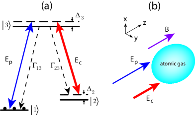
Figure 1: (Color online) (a): Energy-level diagram and excitation scheme of $\Lambda$-type three-level atoms interacting with a weak, pulsed probe field $E_{p}$ and a strong, continuous-wave control field $E_{c}$. $\Delta_{2}$ and $\Delta_{3}$ are the two- and one-photon detunings, respectively. $\Gamma_{13}$ ($\Gamma_{23}$) is the decay rate from $|3\rangle$ to $|1\rangle$ ($|3\rangle$ to $|2\rangle$). The initially populated atoms are indicated by black dots. (b): The coordinate frame and geometrical arrangement of the system. $B$ is the SG gradient magnetic field applied to the atomic gas.

interacting resonantly with a strong, continuous-wave control field of angular frequency $\omega_{c}$ that drives the transition $|2\rangle\leftrightarrow|3\rangle$ and a weak, pulsed probe field (with the time duration $\tau_{0}$ and beam radius $R$ at the entrance of the medium) of center angular frequency $\omega_{p}$ that drives the transition $|1\rangle\leftrightarrow|3\rangle$, respectively; see Fig. 1(a). The electric-field vector of the system can be written as $\mathbf{E}=\mathbf{E}_{p}+\mathbf{E}_{c}=\sum_{l=c,p}{\mathbf{e}_{l}\mathcal{E}}_{l}\exp[i(k_{l}z-\omega_{l}t)]+{\rm c.c}.$, where $\mathbf{e}_{c}$ and $\mathbf{e}_{p}$ ($\mathcal{E}_{c}$ and $\mathcal{E}_{p}$) are, respectively, the polarization unit vectors (envelopes) of the control and probe fields. For simplicity, both the probe and control fields are assumed to propagate along $z$ direction.

Meanwhile, a SG gradient magnetic field with the form

$${\bf B}(x,y)=\hat{\bf z}B(x,y)=\hat{\bf z}(B_{1}x+B_{2}y),$$ (1)

is applied to the system. Here $\hat{\bf z}$ is the unit vector in the $z$ direction, $B_{1}$ and $B_{2}$ are constants characterizing the magnitudes of the gradient in $x$ and $y$ directions, respectively. Due to the presence of ${\bf B}$, Zeeman level shift $\Delta E_{j,\rm Zeeman}=\mu_{B}g_{F}^{j}m_{F}^{j}B$ occurs for all levels. Here $\mu_{B}$, $g_{F}^{j}$, and $m_{F}^{j}$ are Bohr magneton, gyromagnetic factor, and magnetic quantum number of level $|j\rangle$, respectively. The aim of introducing the SG gradient magnetic field (1) is to provide an external potential to control the accelerating motion of Airy optical bullets formed in the probe field (see Sec. III.3 and Sec. IV below). Note that this technique was also used in a recent study of SG deflection of slow light and slow-light solitons KW ; hang . A possible geometrical arrangement of the system is shown in Fig. 1(b).

Under electric-dipole and rotating-wave approximations, the equations of motion for the density matrix elements in interaction picture are given by boyd

$$i\frac{\partial}{\partial t}\sigma_{11}-i\Gamma_{13}\sigma_{33}+\Omega_{p}^{\ast}\sigma_{31}-\Omega_{p}\sigma_{31}^{\ast}=0,$$ (2a)

$$i\frac{\partial}{\partial t}\sigma_{22}-i\Gamma_{23}\sigma_{33}+\Omega_{c}^{\ast}\sigma_{32}-\Omega_{c}\sigma_{32}^{\ast}=0,$$ (2b)

$$i\frac{\partial}{\partial t}\sigma_{33}+i\Gamma_{3}\sigma_{33}-\Omega_{p}^{\ast}\sigma_{31}+\Omega_{p}\sigma_{31}^{\ast}-\Omega_{c}^{\ast}\sigma_{32}+\Omega_{c}\sigma_{32}^{\ast}=0,$$ (2c)

$$\left(i\frac{\partial}{\partial t}+d_{21}\right)\sigma_{21}-\Omega_{p}\sigma_{32}^{\ast}+\Omega_{c}^{\ast}\sigma_{31}=0,$$ (2d)

$$\left(i\frac{\partial}{\partial t}+d_{31}\right)\sigma_{31}-\Omega_{p}(\sigma_{33}-\sigma_{11})+\Omega_{c}\sigma_{21}=0,$$ (2e)

$$\left(i\frac{\partial}{\partial t}+d_{32}\right)\sigma_{32}-\Omega_{c}(\sigma_{33}-\sigma_{22})+\Omega_{p}\sigma_{21}^{\ast}=0,$$ (2f)

where the Rabi frequencies of the probe and control fields are defined, respectively, by $\Omega_{p}=\mathbf{e}_{p}\cdot\mathbf{p}_{31}\mathcal{E}_{p}/\hbar$ and $\Omega_{c}=\mathbf{e}_{c}\cdot\mathbf{p}_{32}\mathcal{E}_{c}/\hbar$, with $\mathbf{p}_{jl}$ being the electric dipole matrix element associated with the transition from states $|l\rangle$ to $|j\rangle$. In Eq. (2), we have also defined $d_{21}=\Delta_{2}+i\gamma_{21}$, $d_{31}=\Delta_{3}+i\gamma_{31}$, and $d_{32}=(\Delta_{3}-\Delta_{2})+i\gamma_{32}$. Here $\Delta_{2}=(\omega_{p}-\omega_{c}-\omega_{21})+\mu_{21}B$ and $\Delta_{3}=(\omega_{p}-\omega_{31})+\mu_{31}B$ are, respectively, the two- and one-photon detunings, with $\mu_{jl}=\mu_{B}(g_{F}^{j}m_{F}^{j}-g_{F}^{l}m_{F}^{l})/\hbar$ and $\omega_{jl}=(E_{j}-E_{l})/\hbar$ ($E_{j}$ is the eigenenergy of the state $|j\rangle$). The composite decay rate $\gamma_{jl}$ in $d_{jl}$ is given by $\gamma_{jl}=(\Gamma_{j}+\Gamma_{l})/2+\gamma_{jl}^{\rm col}$. Here $\Gamma_{j}=\sum_{j<l}\Gamma_{jl}$, with $\Gamma_{jl}$ being the spontaneous emission decay rate from $|l\rangle$ to $|j\rangle$ and $\gamma_{jl}^{\rm col}$ being the dephasing rate reflecting the loss of phase coherence between $|j\rangle$ and $|l\rangle$ without changing of population boyd .

The equation of motion for $\Omega_{p}$ can be obtained by the Maxwell equation, which under the slowly-varying envelope approximation reads

$$i\left(\frac{\partial}{\partial z}+\frac{1}{c}\frac{\partial}{\partial t}\right)\Omega_{p}+\frac{c}{2\omega_{p}}\left(\frac{\partial^{2}}{\partial x^{2}}+\frac{\partial^{2}}{\partial y^{2}}\right)\Omega_{p}+\kappa_{13}\sigma_{31}=0,$$ (3)

where $\kappa_{13}=N_{a}\omega_{p}|\mathbf{p}_{13}|^{2}/(2\varepsilon_{0}c\hbar)$ with $N_{a}$ being atomic concentration.

The above model can be easily realized in realistic physical systems. One of candidates is a cold ⁸⁵Rb atomic gas with energy-levels assigned as $|1\rangle=|5^{2}S_{1/2},F=2,m_{F}=0\rangle$ ($g_{F}=-1/3$), $|2\rangle=|5^{2}S_{1/2},F=3,m_{F}=2\rangle$ ($g_{F}=1/3$), and $|3\rangle=|5^{2}P_{1/2},F=3,m_{F}=1\rangle$ ($g_{F}=1/9$). Then the probe field is $\sigma^{+}$-polarized while the control field is $\sigma^{-}$-polarized. The decay rates are given by $\Gamma_{13}\approx\Gamma_{23}\approx\pi\times 5.75$ MHz, $\gamma_{13}^{\rm col}\approx\gamma_{23}^{\rm col}\approx 1$ kHz, and $|{\bf p}_{13}|=2.54\times 10^{-27}$ C cm Steck . The atomic concentration is taken as $N_{a}=3.67\times 10^{10}$ cm^-3, and hence $\kappa_{13}$ takes the value of $1.0\times 10^{9}$ cm^-1s^-1. All calculations given below will be based on these physical parameters.

III Slow-light Airy wave packets in the absence of dispersion

III.1 Envelope equation

One of the main aims of the present work is to obtain shape-preserving Airy light wave packets without using any external potential note01 . To this end, we first derive an envelope equation in the absence of dispersion based on the Maxwell-Bloch (MB) Eqs. (2) and (3).

We take the following asymptotic expansions $\sigma_{jk}=\delta_{j1}\delta_{k1}+\epsilon\sigma_{jk}^{(l)}+\epsilon^{2}\sigma_{jk}^{(2)}$ ($j,\,k=1,\,2,\,3$; both $\delta_{j1}$ and $\delta_{k1}$ are Kronecker delta symbols), $\Omega_{p}=\epsilon\Omega_{p}^{(1)}+\epsilon^{2}\Omega_{p}^{(2)}$, $d_{j1}=d_{j1}^{(0)}+\epsilon d_{j1}^{(1)}$ ($j=2,\,3$), and $d_{32}=d_{32}^{(0)}+\epsilon d_{32}^{(1)}$, where $\epsilon$ is a dimensionless small parameter characterizing the amplitude of the probe field. All quantities on the right hand side of the expansions are assumed as functions of the multi-scale variables $z_{2j}=\epsilon^{j}z$, $t_{2j}=\epsilon^{j}t$ ($j=0,1$), $x_{1}=\epsilon^{1/2}x$, and $y_{1}=\epsilon^{1/2}y$. Additionally, we assume the gradient of the SG magnetic field is of $\epsilon^{3/2}$ order, and hence $B(x,y)=\epsilon(B_{1}^{(1)}x_{1}+B_{2}^{(1)}y_{1})$. Thus we have $d_{21}^{(0)}=(\omega_{p}-\omega_{c}-\omega_{21})+i\gamma_{21}$, $d_{31}^{(0)}=(\omega_{p}-\omega_{31})+i\gamma_{31}$, $d_{32}^{(0)}=(\omega_{c}-\omega_{32})+i\gamma_{32}$, $d_{21}^{(1)}=\mu_{21}(B_{1}^{(1)}x_{1}+B_{2}^{(1)}y_{1})$, $d_{31}^{(1)}=\mu_{31}(B_{1}^{(1)}x_{1}+B_{2}^{(1)}y_{1})$, and $d_{32}^{(1)}=\mu_{32}(B_{1}^{(1)}x_{1}+B_{2}^{(1)}y_{1})$.

Substituting the expansions into the MB Eqs. (2) and (3), and comparing the coefficients of $\epsilon^{l}$ ($l=1,2\cdots$), we obtain a set of linear but inhomogeneous equations which can be solved order by order.

At leading order ($l=1$, i.e. the terms of order of $\epsilon$), we get the solution

$$\Omega_{p}=Fe^{i[K(\omega)z-\omega t]},$$ (4a)

$$\sigma_{j1}=\frac{\delta_{j3}(\omega+d_{21}^{(0)})-\delta_{j2}\Omega_{c}^{\ast}}{D(\omega)}Fe^{i[K(\omega)z-\omega t]}\quad(j=2,3),$$ (4b)

where $D(\omega)=|\Omega_{c}|^{2}-(\omega+d_{21}^{(0)})(\omega+d_{31}^{(0)})$ and $F$ is a yet to be determined envelope function of the slow variables $t_{2}$, $x_{1}$, $y_{1}$, and $z_{2}$. The dependence of $K$ on $\omega$ note1 obeys the linear dispersion relation

$$K(\omega)=\frac{\omega}{c}+\kappa_{13}\frac{\omega+d_{21}^{(0)}}{D(\omega)}.$$ (5)

In Fig. 2(a)

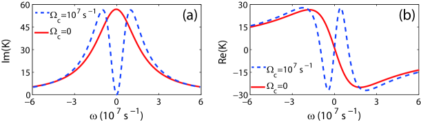
Figure 2: (Color online) Im$(K)$ (a) and Re$(K)$ (b) as functions of $\omega$, respectively. The dashed and solid lines in each panel correspond to the presence ($\Omega_{c}=1.0\times 10^{7}$ ${\rm s}^{-1}$) and the absence ($\Omega_{c}=0$) of the control field, respectively.

and Fig. 2(b) we have plotted the real and imaginary parts of $K$, i.e. Re$(K)$ and Im$(K)$, as functions of $\omega$ for the exact one- and two-photon resonances ($\omega_{p}-\omega_{c}-\omega_{21}=\omega_{p}-\omega_{31}=0$). The solid and dashed lines in the figure correspond, respectively, to the absence ($\Omega_{c}=0$) and the presence ($\Omega_{c}=1.0\times 10^{7}$ ${\rm s}^{-1}$) of the control field. One sees that when $\Omega_{c}=0$, the probe field suffers maximum absorption at $\omega=0$ (the solid line of Fig. 2(a) ). However, when $\Omega_{c}\neq 0$ and satisfies the condition $|\Omega_{c}|^{2}\gg\gamma_{21}\gamma_{31}$, a transparency window is opened in the probe-field absorption spectrum nearly $\omega=0$ (the dashed line of Fig. 2(a) ), and hence the probe field can propagate in the system with nearly vanishing absorption, which is a typical character of EIT. In addition, for the large control field the slope of Re$(K)$ is drastically changed and steepened around $\omega=0$ (see the dashed line of Fig. 2(b) ) which results in a significant reduction of the group velocity of the probe field, $V_{g}\equiv{\rm Re}[(\partial K/\partial\omega)^{-1}]\approx|\Omega_{c}|^{2}/\kappa_{13}$, and hence slow light (see Eq. (9) below). These interesting characters are due to the quantum destructive interference (EIT) effect induced by the control field fle .

At next order ($l=2$, i.e. the terms of order of $\epsilon^{2}$), a divergence-free condition requires the equation for the envelope function $F$:

$$i\left(\frac{\partial}{\partial z_{2}}+\frac{1}{V_{g}}\frac{\partial}{\partial t_{2}}\right)F+\frac{c}{2\omega_{p}}\left(\frac{\partial^{2}}{\partial x_{1}^{2}}+\frac{\partial^{2}}{\partial y_{1}^{2}}\right)F+P(x_{1},y_{1})F=0.$$ (6)

where $V_{g}\equiv{\rm Re}[(\partial K/\partial\omega)^{-1}]$ is the group velocity of the envelope $F$, and

$$P(x_{1},y_{1})=\kappa_{13}\frac{|\Omega_{c}|^{2}\mu_{21}+(\omega+d_{21}^{(0)})^{2}\mu_{31}}{D^{2}(\omega)}(B_{1}^{(1)}x_{1}+B_{2}^{(1)}y_{1})$$

provides an external potential for $F$, resulted from the SG gradient magnetic field (1).

Equation (6) can be written into the dimensionless form

$$i\left(\frac{\partial}{\partial s}+\lambda\frac{\partial}{\partial\tau}\right)U+\frac{1}{2}\left(\frac{\partial^{2}}{\partial\xi^{2}}+\frac{\partial^{2}}{\partial\eta^{2}}\right)U+Q(\xi,\eta)U=0,$$ (7)

with

$$\lambda=L_{\rm Diff}/(V_{g}\tau_{0}),$$ (8)

where $s=z/L_{\rm Diff}$ ($L_{\rm Diff}=\omega_{p}R^{2}/c$ being the characteristic diffraction length), $\tau=t/\tau_{0}$ ($\tau_{0}$ being the typical duration of the probe filed), $(\xi,\eta)=(x,y)/R$ ($R$ being the typical transverse radius of the probe filed), $U=\Omega_{p}/U_{0}$ ($U_{0}$ being the typical Rabi frequency of the probe filed), and $Q(\xi,\eta)=P(x_{1},y_{1})L_{\rm Diff}$. We have also assumed that the imaginary part of the coefficients in the equation is much smaller than the corresponding real part. This assumption is allowed because of the existence of the EIT effect induced by the control field (also see the example given below).

For the convenience of following discussions, we focus on a particular example under a set of realistic parameters: $\Omega_{c}=1.6\times 10^{7}$ s^-1, $\omega_{p}-\omega_{c}-\omega_{21}=8.0\times 10^{5}$ s^-1, $\omega_{p}-\omega_{31}=-4.0\times 10^{7}$ s^-1, and $R=4.78\times 10^{-3}$ cm with other parameters being the same with those used in the last paragraph of Sec. II. Then we obtain $K|_{\omega=0}=2.77+i0.14$ cm^-1 and $\partial K/\partial\omega|_{\omega=0}=(3.07+i0.31)\times 10^{-6}$ cm^-1 s. We see that the imaginary part of these quantities is indeed much smaller than their corresponding real part. Furthermore, the dispersion length $L_{\rm Diff}=1.81$ cm and the group velocity

$$V_{g}\approx 1.07\times 10^{-5}c.$$ (9)

Thus the probe filed indeed propagates with a very low group velocity in $z$ direction which is due to the EIT effect contributed by the control field.

Note that group-velocity dispersion term (i.e. the term proportional to $\partial^{2}U/\partial\tau^{2}$) does not appears in Eq. (7). Thus such equation is valid only for the probe filed with a large $\tau_{0}$. To estimate the order of magnitude of $\tau_{0}$ for which the dispersion is negligible, we compare the characteristic dispersion length (defined by $L_{\rm Disp}={\rm Re}(\tau_{0}^{2}/|\partial^{2}K/\partial\omega^{2}|_{\omega=0}$) and the diffraction length $L_{\rm Diff}$ defined above. By setting $L_{\rm Disp}=L_{\rm Diff}=1.81$ cm we obtain $\tau_{0}=1.28\times 10^{-6}$ s. Consequently, if $\tau_{0}$ is much larger than $1.28\times 10^{-6}$ s, $L_{\rm Disp}$ will be much longer than $L_{\rm Diff}$ and the dispersion effect of the system can be neglected safely.

III.2 Slow-light Airy wave packet solutions

We now seek slow-light Airy wave packet solutions of Eq. (7) for the absence of the SG gradient magnetic field note01 , i.e. $B_{1}=B_{2}=0$ and hence $Q=0$.

Since Eq. (7) is a linear one, we can solve it by taking guo

$$U(\tau,\xi,\eta,s)=\psi(\tau,s)\phi(\tau,\xi,\eta),$$ (10)

with

$$\psi(\tau,s)=\frac{1}{\sqrt[4]{2\pi\rho^{2}}}e^{-(s-\tau/\lambda)^{2}/(4\rho^{2})}=\frac{1}{\sqrt[4]{2\pi\rho^{2}}}e^{-(z-V_{g}t)^{2}/(4\rho^{2}L_{\rm Diff}^{2})},$$ (11)

where $\rho$ is a free real parameter. When writing Eq. (11) we have assumed that the probe-field envelope is a Gaussian pulse propagating in $z$ direction with velocity $V_{g}$.

In this way, $\phi(\tau,\xi,\eta)$ satisfies the following equation

$$i\lambda\frac{\partial}{\partial\tau}\phi+\frac{1}{2}\left(\frac{\partial^{2}}{\partial\xi^{2}}+\frac{\partial^{2}}{\partial\eta^{2}}\right)\phi=0.$$ (12)

Taking $\phi(\tau,\xi,\eta)=\phi_{1}(\tau,\xi)\phi_{2}(\tau,\eta)$, Eq. (12) can be further decomposed into

$$i\lambda\frac{\partial\phi_{1}}{\partial\tau}+\frac{1}{2}\frac{\partial^{2}\phi_{1}}{\partial\xi^{2}}=0,$$ (13a)

$$i\lambda\frac{\partial\phi_{2}}{\partial\tau}+\frac{1}{2}\frac{\partial^{2}\phi_{2}}{\partial\eta^{2}}=0,$$ (13b)

which admit the Airy function solutions $\phi_{1}(\tau,\xi)={\rm Ai}[\xi-\tau^{2}/(4\lambda^{2})]e^{i[\xi/2-\tau^{2}/(12\lambda^{2})]\tau/\lambda}$ and $\phi_{2}(\tau,\eta)={\rm Ai}[\eta-\tau^{2}/(4\lambda^{2})]e^{i[\eta/2-\tau^{2}/(12\lambda^{2})]\tau/\lambda}$, respectively. Here ${\rm Ai}$ is the Airy function Berry . Thus, we have $\phi(\tau,\xi,\eta)={\rm Ai}[\xi-\tau^{2}/(4\lambda^{2})]{\rm Ai}[\eta-\tau^{2}/(4\lambda^{2})]e^{i[\xi/2+\eta/2-\tau^{2}/(6\lambda^{2})]\tau/\lambda}$. The Airy wave packet has the property that its intensity profile remains invariant but experiences a constant acceleration in both $x$ and $y$ directions during propagation Berry ; greenb ; Siviloglou1 .

An ideal Airy wave packet, however, is not square integrable, i.e. $\int{\rm Ai}^{2}(x)dx\rightarrow\infty$, which means that it has infinite energy. The reason comes from the fact that the tail of the Airy function decays very slowly. Thus, it is not possible to generate an ideal Airy wave packet experimentally. One suitable way to solve this problem is to use a finite-energy Airy wave packet by introducing an additional exponential aperture function, i.e. by taking the initial condition as the form of $\phi(0,\xi,\eta)={\rm Ai}(\xi){\rm Ai}(\eta)e^{a_{1}\xi+a_{2}\eta}$. Here $a_{j}$ ($j=1,\,2$) are positive parameters so as to ensure containment of the infinite Airy tail. Typically, $a_{j}\ll 1$ so the resulting profile of the function closely resembles that of the intended Airy function Siviloglou1 . Such finite-energy Airy wave packets have been recently demonstrated in experiment Siviloglou2 . By directly integrating Eq. (12) we have

$$\phi(\tau,\xi,\eta) = {\rm Ai}[\xi-\tau^{2}/(4\lambda^{2})+ia_{1}\xi]{\rm Ai}[\eta-\tau^{2}/(4\lambda^{2})+ia_{2}\eta]e^{i[\xi/2+\eta/2-\tau^{2}/(6\lambda^{2})]\tau/\lambda}$$ (14)

$$\times e^{a_{1}\xi-a_{1}\xi^{2}/2+ia_{1}^{2}\xi/2}e^{a_{2}\eta-a_{2}\eta^{2}/2+ia_{2}^{2}\eta/2}.$$

The center of the wave packet (14) moves along the trajectory $\xi=\eta=\tau^{2}/(4\lambda^{2})$ and hence tend to freely accelerate during propagation even without any action by external force.

Consequently, the solution of Eq. (7) without the external potential reads

$$U(\tau,\xi,\eta,s) = \frac{1}{\sqrt[4]{2\pi\rho^{2}}}e^{-(s-\tau/\lambda)^{2}/(4\rho^{2})}\,{\rm Ai}[\xi-\tau^{2}/(4\lambda^{2})+ia_{1}\xi]{\rm Ai}[\eta-\tau^{2}/(4\lambda^{2})+ia_{2}\eta]$$ (15)

$$\times e^{i[\xi/2+\eta/2-\tau^{2}/(6\lambda^{2})]\tau/\lambda}e^{a_{1}\xi-a_{1}\xi^{2}/2+ia_{1}^{2}\xi/2}e^{a_{2}\eta-a_{2}\eta^{2}/2+ia_{2}^{2}\eta/2},$$

which consists of two Airy wave packets in $x$ and $y$ directions and a Gaussian pulse in $z$ direction. The center of the probe filed (15) moves along with the trajectory

$$(x(t),y(t),z(t)\,)=\left(\frac{R}{4\lambda^{2}\tau_{0}^{2}}t^{2},\frac{R}{4\lambda^{2}\tau_{0}^{2}}t^{2},V_{g}t\right).$$ (16)

Notice that the solution (15) is localized in all three spatial dimensions and in time, thus it can be considered as a (3+1)D (linear) Airy light bullet realized in the coherent atomic system via EIT, which has an ultraslow propagating velocity in $z$ direction.

The Airy light wave packet obtained above is quite stable. Fig. 3 shows the result of numerical simulation on its

Figure 3: (Color online) (a)-(c) Spatial intensity distributions of the slow-light Airy wave packet in $xy$ plane for $t/\tau_{0}=0$, $2$, and $4$, respectively. (d)-(f) Numerical (dots) and theoretical (solid lines) results of the center positions $x=x(t)$, $y=y(t)$, $z=z(t)$ of the slow-light Airy wave packet. (g)-(i) Intensity isosurfaces of the Airy wave packet for $t/\tau_{0}=0$, $2$, and $4$, respectively.

stability by using split-step Fourier method. In doing this, we have added small random perturbations less than 10% to both amplitude and phase to the solution Eq. (15) and then evolve it according to Eq. (7) with $Q=0$. The values of parameters are given in Sec. III.1 with $\tau_{0}=L_{\rm Diff}/V_{g}=0.56\times 10^{-5}$ s (i.e. $\lambda=1$). Fig. 3(a)-(c) show the spatial distribution of the Airy wave packet in the $xy$ plane for $t/\tau_{0}=0$, $2$, and $4$, respectively. Fig. 3(d)-(f) show the numerical (dots) and theoretical (lines) shifts of the Airy wave packet in the $x$, $y$, and $z$ directions. The accelerating behavior of wave packets in $x$ and $y$ directions is clearly observed. In Fig. 3(g)-(i) we show the intensity isosurfaces of the Airy wave packet for $t/\tau_{0}=0$, $2$, and $4$ in $xyz$ space, respectively. These results clearly demonstrate that the slow-light Airy wave packet obtained in the present system is rather robust up to the propagation time $t=4\tau_{0}\approx 2.24\times 10^{-5}$ s even without any trapping potential. This stability can be explained by the low absorption of the system and the capability of Airy wave packets in $x$ and $y$ directions for withstanding diffraction.

III.3 Acceleration control of the slow-light Airy wave packets

In the paper by Berry and Balazs Berry , motion of an Airy wave packet obeying a (1+1)D Schrödinger equation with a time dependent but spatially uniform force was investigated. Here we extend their study to (3+1)D case and realize an active control of the acceleration by using the SG gradient magnetic field.

The explicit form of the potential in Eq. (7) reads

$$Q(\xi,\eta)=\kappa_{13}\frac{|\Omega_{c}|^{2}\mu_{21}+d_{21}^{(0)\,2}\mu_{31}}{(|\Omega_{c}|^{2}-d_{21}^{(0)}d_{31}^{(0)})^{2}}L_{\rm Disp}R(B_{1}\xi+B_{2}\eta)\equiv Q_{1}\xi+Q_{2}\eta.$$ (17)

We see that the coefficients $Q_{1}$ and $Q_{2}$ are proportional to the gradient of the SG magnetic field in $x$ and $y$ directions, respectively. With such potential, Eq. (13) are replaced by

$$i\lambda\frac{\partial\phi_{1}}{\partial\tau}+\frac{1}{2}\frac{\partial^{2}\phi_{1}}{\partial\xi^{2}}+Q_{1}\xi\phi_{1}=0,$$ (18a)

$$i\lambda\frac{\partial\phi_{2}}{\partial\tau}+\frac{1}{2}\frac{\partial^{2}\phi_{2}}{\partial\eta^{2}}+Q_{2}\eta\phi_{2}=0.$$ (18b)

Using the transformation $\phi_{1}=\phi_{1}^{\prime}e^{i[Q_{1}\xi^{\prime}+Q_{1}^{2}\tau^{2}/(3\lambda^{2})]\tau/\lambda}$ and $\phi_{2}=\phi_{2}^{\prime}e^{i[Q_{2}\eta^{\prime}+Q_{2}^{2}\tau^{2}/(3\lambda^{2})]\tau/\lambda}$ with $\xi^{\prime}=\xi-Q_{1}\tau^{2}/(2\lambda^{2})$ and $\eta^{\prime}=\eta-Q_{2}\tau^{2}/(2\lambda^{2})$, Eq. (18) is converted into $i\lambda\partial\phi_{1}^{\prime}/\partial\tau+(1/2)\partial^{2}\phi_{1}^{\prime}/\partial\xi^{\prime 2}=0$ and $i\lambda\partial\phi_{2}^{\prime}/\partial\tau+(1/2)\partial^{2}\phi_{2}^{\prime}/\partial\eta^{\prime 2}=0$. Thus we can obtain the Airy function solutions of Eq. (18) as $\phi_{1}(\tau,\xi^{\prime})={\rm Ai}[\xi^{\prime}-\tau^{2}/(4\lambda^{2})]e^{i[\xi^{\prime}/2-\tau^{2}/(12\lambda^{2})]\tau/\lambda}e^{i[Q_{1}\xi^{\prime}+Q_{1}^{2}\tau^{2}/(3\lambda^{2})]\tau/\lambda}$ and $\phi_{2}(\tau,\eta^{\prime})={\rm Ai}[\eta^{\prime}-\tau^{2}/(4\lambda^{2})]e^{i[\eta^{\prime}/2-\tau^{2}/(12\lambda^{2})]\tau/\lambda}e^{i[Q_{2}\eta^{\prime}+Q_{2}^{2}\tau^{2}/(3\lambda^{2})]\tau/\lambda}$, and hence $\phi(\tau,\xi^{\prime},\eta^{\prime})=\phi_{1}(\tau,\xi^{\prime})\phi_{2}(\tau,\eta^{\prime})={\rm Ai}[\xi^{\prime}-\tau^{2}/(4\lambda^{2})]{\rm Ai}[\eta^{\prime}-\tau^{2}/(4\lambda^{2})]e^{i[\xi^{\prime}/2+\eta^{\prime}/2-\tau^{2}/(6\lambda^{2})]\tau/\lambda}e^{i[Q_{1}\xi^{\prime}+Q_{2}\eta^{\prime}+Q_{1}^{2}\tau^{2}/(3\lambda^{2})+Q_{2}^{2}\tau^{2}/(3\lambda^{2})]\tau/\lambda}$. A finite-energy Airy function solution reads

$$\phi(\tau,\xi^{\prime},\eta^{\prime}) = {\rm Ai}[\xi^{\prime}-\tau^{2}/(4\lambda^{2})+ia_{1}\xi^{\prime}]{\rm Ai}[\eta^{\prime}-\tau^{2}/(4\lambda^{2})+ia_{2}\eta^{\prime}]e^{i[\xi^{\prime}/2+\eta^{\prime}/2-\tau^{2}/(6\lambda^{2})]\tau/\lambda}$$ (19)

$$\times e^{a_{1}\xi^{\prime}-a_{1}\xi^{\prime 2}/2+ia_{1}^{2}\xi^{\prime}/2}e^{a_{2}\eta^{\prime}-a_{2}\eta^{\prime 2}/2+ia_{2}^{2}\eta^{\prime}/2}e^{i[Q_{1}\xi^{\prime}+Q_{2}\eta^{\prime}+Q_{1}^{2}\tau^{2}/(3\lambda^{2})+Q_{2}^{2}\tau^{2}/(3\lambda^{2})]\tau/\lambda}.$$

Consequently, the Airy light wave packet solution of Eq. (7) with the potential (17) is given by

$$U(\tau,\xi^{\prime},\eta^{\prime},s) = \frac{1}{\sqrt[4]{2\pi\rho^{2}}}e^{-(s-\tau/\lambda)^{2}/(4\rho^{2})}\,{\rm Ai}[\xi^{\prime}-\tau^{2}/(4\lambda^{2})+ia_{1}\xi^{\prime}]{\rm Ai}[\eta^{\prime}-\tau^{2}/(4\lambda^{2})+ia_{2}\eta^{\prime}]$$ (20)

$$\times e^{i[\xi^{\prime}/2+\eta^{\prime}/2-\tau^{2}/(6\lambda^{2})]\tau/\lambda}e^{a_{1}\xi^{\prime}-a_{1}\xi^{\prime 2}/2+ia_{1}^{2}\xi^{\prime}/2}e^{a_{2}\eta^{\prime}-a_{2}\eta^{\prime 2}/2+ia_{2}^{2}\eta^{\prime}/2}$$

$$\times e^{i[Q_{1}\xi^{\prime}+Q_{2}\eta^{\prime}+Q_{1}^{2}\tau^{2}/(3\lambda^{2})+Q_{2}^{2}\tau^{2}/(3\lambda^{2})]\tau/\lambda}.$$

It is clear that the motional trajectory of the Airy wave packet (20) in the presence of the SG gradient magnetic field is given by $\xi=[\tau^{2}/(2\lambda^{2})](1/2+Q_{1})$, $\eta=[\tau^{2}/(2\lambda^{2})](1/2+Q_{2})$, and $s=\tau/\lambda$, i.e.

$$(x(t),y(t),z(t)\,)=\left(\frac{R}{2\lambda^{2}\tau_{0}^{2}}\left(\frac{1}{2}+Q_{1}\right)t^{2},\frac{R}{2\lambda^{2}\tau_{0}^{2}}\left(\frac{1}{2}+Q_{2}\right)t^{2},V_{g}t\right).$$ (21)

Obviously, the magnitude and direction of the acceleration of the slow-light Airy wave packet in the $xy$ plane can be easily controlled by changing the gradient of the SG magnetic field, i.e. by changing the magnitude of $Q_{1}$ and $Q_{2}$. Particularly, when taking $Q_{1}=Q_{2}=-1/2$ corresponding to the magnetic gradients $B_{1}=B_{2}\approx-3.19$ G cm^-1 (the minus sign here means the SG magnetic field should be applied along $-z$ direction), the trajectory of the Airy wave packet becomes $(\xi,\eta)=(0,0)$. This means that the force provided by the SG magnetic field in each transverse direction is sufficient to overcome the acceleration in this direction, i.e. the transverse motion of the wave packet can be completely stopped. As a result, the Airy wave packet moves along $z$ direction with the ultraslow velocity $V_{g}$.

Additional control of the transverse motion of the Airy wave packet is also possible. In fact, if the SG gradient magnetic field is chosen to be time-dependent, i.e. $Q_{1}=Q_{1}(\tau)$ and $Q_{2}=Q_{2}(\tau)$, the transverse trajectory of the Airy wave packet becomes

$$\xi=\frac{1}{\lambda^{2}}\left[\frac{\tau^{2}}{4}+\int_{0}^{\tau}Q_{1}(\tau^{\prime})(\tau-\tau^{\prime})d\tau^{\prime}\right],$$ (22a)

$$\eta=\frac{1}{\lambda^{2}}\left[\frac{\tau^{2}}{4}+\int_{0}^{\tau}Q_{2}(\tau^{\prime})(\tau-\tau^{\prime})d\tau^{\prime}\right].$$ (22b)

Particularly, when taking $Q_{1}=-1/2+V_{1}\delta(\tau)$ and $Q_{2}=-1/2$, the trajectory of the Airy wave packet is given by $(\xi,\eta,s)=(V_{1}\tau/\lambda^{2},0,\tau/\lambda)$. This means that the wave packet propagates with a constant velocity $V_{1}R/(\lambda^{2}\tau_{0})$ in the $x$ direction and locates at zero in the $y$ direction. Furthermore, if taking $Q_{1}=-1/2+V_{1}\delta(\tau)$ and $Q_{2}=-1/2+V_{2}\delta(\tau)$, the trajectory of the wave packet turns to $(\xi,\eta,s)=(V_{1}\tau/\lambda^{2},V_{2}\tau/\lambda^{2},\tau/\lambda)$, i.e. it propagates with constant velocities $V_{1}R/(\lambda^{2}\tau_{0})$ and $V_{2}R/(\lambda^{2}\tau_{0})$ in $x$ and $y$ directions, respectively.

Shown in Fig. 4 is the trajectory control of the slow-light Airy wave packets by changing the values of $V_{1}$ and $V_{2}$. The values of parameters are the same with those used in Fig. 3. In Fig. 4(a)-(c) we show spatial distributions of the Airy wave packet in the $xy$ plane at $t/\tau_{0}=4$ for $(V_{1},V_{2})=(0,0)$, $(V_{1},V_{2})=(1,0)$, and $(V_{1},V_{2})=(1,1)$, respectively. Fig. 4(c) shows the corresponding 3D trajectory plots of Airy wave packets respectively for $(V_{1},V_{2})=(0,0)$ (dotted line), $(V_{1},V_{2})=(1,0)$ (dashed line), and $(V_{1},V_{2})=(1,1)$ (solid line) with the fixed atomic medium length $4L_{\rm Diff}\approx 7.24$ cm. The center positions of Airy wave packets when exiting the medium are $(0,0)$, $(4,0)$, and $(4,4)$, respectively.

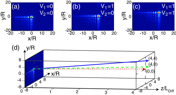
Figure 4: (Color online) (a)-(c): Spatial intensity distributions of the slow-light Airy wave packet in $xy$ plane at $t/\tau_{0}=4$ for $(V_{1},V_{2})=(0,0)$, $(V_{1},V_{2})=(1,0)$, and $(V_{1},V_{2})=(1,1)$, respectively. (d): The 3D trajectory plots of Airy wave packets for $(V_{1},V_{2})=(0,0)$ (dotted line), $(V_{1},V_{2})=(1,0)$ (dashed line), and $(V_{1},V_{2})=(1,1)$ (solid line). The medium length is fixed to be $4L_{\rm Diff}\approx 7.24$ cm. The center positions of Airy wave packets when exiting the medium are $(0,0)$, $(4,0)$, and $(4,4)$, respectively.

One can also obtain easily other different motional trajectories of the slow-light Airy wave packet by using different SG gradient magnetic field, which are not shown here.

IV Slow-light Airy wave packets in the presence of dispersion

The results presented in the last section are valid only for large time duration of the probe filed, i.e for large $\tau_{0}$. If $\tau_{0}$ becomes smaller, the dispersion effect of the system is significant and hence must be taken into account. In this case, the envelope equation (7) is not valid. To get an envelope equation valid for the presence of dispersion, the multi-scale variables used in Sec. III.1 should be replaced by $z_{j}=\epsilon^{j/2}z$ ($j=0,1,2$), $t_{j}=\epsilon^{j/2}t$ ($j=0,1$), $x_{1}=\epsilon^{1/2}x$, and $y_{1}=\epsilon^{1/2}y$. Then, at the leading order ($l=1$, i.e. the terms of order of $\epsilon$), we have the same solutions with those given in Eqs. (4) and (5) in Sec III.1. At next order ($l=2$, i.e. the terms of order of $\epsilon^{3/2}$), a divergence-free condition requires $\partial F/\partial z_{1}+(1/V_{g})\partial F/\partial t_{1}=0$. The divergence-free condition at the third order ($l=3$, i.e. the terms of order of $\epsilon^{2}$) yields the equation for the envelope function $F$:

$$i\frac{\partial}{\partial z_{2}}F-\frac{1}{2}\frac{\partial^{2}K}{\partial\omega^{2}}\frac{\partial^{2}}{\partial t_{1}^{2}}F+\frac{c}{2\omega_{p}}\left(\frac{\partial^{2}}{\partial x_{1}^{2}}+\frac{\partial^{2}}{\partial y_{1}^{2}}\right)F+P(x_{1},y_{1})F=0.$$ (23)

Combining the equations of all orders and returning to original variables, we obtain the equation in the dimensionless form

$$i\frac{\partial}{\partial s}U+\frac{1}{2}\left(\mu\frac{\partial^{2}}{\partial\sigma^{2}}+\frac{\partial^{2}}{\partial\xi^{2}}+\frac{\partial^{2}}{\partial\eta^{2}}\right)U+Q(\xi,\eta)U=0,$$ (24)

with $\sigma=(t-z/V_{g})/\tau_{0}$ and $\mu=-{\rm sign}[{\rm Re}(\partial^{2}K/\partial\omega^{2}|_{\omega=0})]L_{\rm Diff}/L_{\rm Disp}$. The quantities $s$, $\xi$, $\eta$, $U$, and $Q$ have the same definitions as those in given Eq. (7).

With the parameters given in Sec. III.1 and by taking $\tau_{0}=1.28\times 10^{-6}$ s (which is the critical value for which the dispersion effect must be considered; see the last paragraph of Sec. III.1), we obtain $K_{2}=(-0.87+i0.26)\times 10^{-12}$ cm^-1 s² which leads to $L_{\rm Disp}=L_{\rm Diff}=1.81$ cm, and hence $\mu=1$.

In the absence of the SG gradient magnetic field (i.e. $Q=0$), by using a similar method in Sec. III.2 we obtain the Airy wave packet solution of Eq. (24)

$$U(\sigma,\xi,\eta,s) = {\rm Ai}(\sigma-s^{2}/4+ia_{0}\sigma)\,{\rm Ai}(\xi-s^{2}/4+ia_{1}\xi)\,{\rm Ai}(\eta-s^{2}/4+ia_{2}\eta)$$ (25)

$$\times e^{i(\sigma/2+\xi/2+\eta/2-s^{2}/4)s}e^{a_{0}\sigma-a_{0}\sigma^{2}/2+ia_{0}^{2}\sigma/2}e^{a_{1}\xi-a_{1}\xi^{2}/2+ia_{1}^{2}\xi/2}$$

$$\times e^{a_{2}\eta-a_{2}\eta^{2}/2+ia_{2}^{2}\eta/2},$$

which consists of two Airy beams in $x$ and $y$ directions and a longitudinal Airy wave packet propagating in $z$ direction note2 . Different from the solution (15), the center of the Airy wave packet given by (25) moves along the trajectory $\xi=\eta=\sigma=s^{2}/4$. That is, in $x$ and $y$ directions

$$(x(z),y(z)\,)=\left(\frac{R}{4L_{\rm Diff}^{2}}z^{2},\frac{R}{4L_{\rm Diff}^{2}}z^{2}\right),$$ (26)

and in $z$ direction

$$z(t)=2L_{\rm Diff}\left(\sqrt{\frac{t}{\tau_{0}}+\lambda^{2}}-\lambda\right),$$ (27)

where $\lambda$ is defined by Eq. (8). Thus the propagating velocity of the Airy wave packet in $z$ direction is

$$V_{z}=\frac{V_{g}}{z/(2\lambda L_{\rm Diff})+1}.$$ (28)

From Eq. (26), we see that the Airy light wave packet (25) has stationary, but bent beam intensity distributions in the transverse $x$ and $y$ directions; in the longitudinal $z$ direction it however is a Airy spatial-temporal wave packet with the propagating velocity $V_{z}$, which is proportional to $V_{g}$ (Eq. (28) ). Interestingly, $V_{z}$ can be further reduced when the propagating distance $z$ becomes large. For instance, with the given parameters we have $\lambda=4.38$, and hence we obtain $V_{z}=0.68V_{g}$ when $z=4L_{\rm Diff}$.

Shown in Fig. 5 is the result of a numerical simulation of the slow-light Airy wave packet in the presence of dispersion. In the simulation,

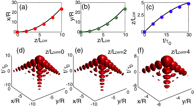
Figure 5: (Color online) (a)-(c) The numerical (dots) and theoretical (lines) results of the center positions $x=x(z)$, $y=y(z)$, $z=z(t)$ of the show-light Airy wave packet in the presence of dispersion. (d)-(f) Intensity isosurfaces of the show-light Airy wave packet for $z/L_{\rm Diff}=0$, $2$, and $4$, respectively.

to test the stability of the Airy wave packet we have added small random perturbations less than 10% to both amplitude and phase to the solution Eq. (25) and then evolve it according to Eq. (24) with $Q=0$. Plotted in Fig. 5(a)-(c) are the numerical (dots) and theoretical (lines) results on the evolution of the center position $x=x(z)$, $y=y(z)$, $z=z(t)$ of the Airy wave packet. The bending (in $x$ and $y$ directions) and decelerating (in $z$ direction) behavior is clearly observed. In Fig. 5(d)-(f) we show the intensity isosurfaces of the Airy wave packet for $z/L_{\rm Diff}=0$, $2$, and $4$ in $xyt$ space, respectively. These results demonstrate that the slow-light Airy wave packet obtained in the present system is rather robust up to the propagation distance $z=4L_{\rm Diff}\approx 7.24$ cm even without any trapping potential. This stability can be explained by the low absorption and the capability of the Airy wave packet for withstanding both dispersion and diffraction.

In the presence of the SG magnetic field, the slow-light Airy wave packet solution of Eq. (24) with the potential (17) can also be obtained, which reads

$$U(\sigma,\xi^{\prime},\eta^{\prime},s) = {\rm Ai}(\sigma-s^{2}/4+ia_{0}\sigma){\rm Ai}(\xi^{\prime}-s^{2}/4+ia_{1}\xi^{\prime}){\rm Ai}(\eta^{\prime}-s^{2}/4+ia_{2}\eta^{\prime})$$ (29)

$$\times e^{i(\sigma/2+\xi^{\prime}/2+\eta^{\prime}/2-s^{2}/4)s}e^{a_{0}\sigma-a_{0}\sigma^{2}/2+ia_{0}^{2}\sigma/2}e^{a_{1}\xi^{\prime}-a_{1}\xi^{\prime 2}/2+ia_{1}^{2}\xi^{\prime}/2}e^{a_{2}\eta^{\prime}-a_{2}\eta^{\prime 2}/2+ia_{2}^{2}\eta^{\prime}/2}$$

$$\times e^{i(Q_{1}\xi^{\prime}+Q_{2}\eta^{\prime}+Q_{1}^{2}s^{2}/3+Q_{2}^{2}s^{2}/3)s},$$

where $\xi^{\prime}=\xi-Q_{1}s^{2}/2$ and $\eta^{\prime}=\eta-Q_{2}s^{2}/2$. We see that, as in the case without the SG magnetic field (see Eq. (25) ), the Airy wave packet propagates in $z$ direction with the same ultraslow, decreased velocity $V_{z}$ given in Eq. (28). In addition, it has also a stationary intensity distribution bent in $x$ and $y$ directions, but now with a different bending trajectory $\xi=(s^{2}/2)(1/2+Q_{1})$, $\eta=(s^{2}/2)(1/2+Q_{2})$, i.e.

$$(x(z),y(z)\,)=\left(\frac{R}{2L_{\rm Diff}^{2}}\left(\frac{1}{2}+Q_{1}\right)z^{2},\frac{R}{2L_{\rm Diff}^{2}}\left(\frac{1}{2}+Q_{2}\right)z^{2}\,\right).$$ (30)

Obviously, the trajectory bending in the transverse directions of the Airy wave packet can be completely eliminated by using the SG gradient magnetic field. For example, taking $Q_{1}=Q_{2}=-1/2$ one has $(x(z),y(z)\,)=(0,0)$. Similarly, other kinds of active control on the trajectory of Airy wave packets can also be implemented easily by manipulating the SG gradient magnetic field.

V Summary

In this article, we have proposed a scheme to create (3+1)-dimensional slow-light Airy wave packets in a resonant $\Lambda$-type three-level atomic gas via EIT induced by the control field. We have shown that in the absence of dispersion the Airy wave packets obtained consist of two Airy wave packets accelerated in transverse directions and a longitudinal Gaussian pulse with a constant propagating velocity lowered to $10^{-5}\,c$. We have also shown that in the presence of dispersion one is able to create another type of slow-light Airy wave packets consisting of two Airy beams in transverse directions and an Airy wave packet in the longitudinal direction. In this situation, the longitudinal velocity of the Airy wave packets can be further reduced during propagation. In addition, we have demonstrated that the transverse accelerations (or bending) of the both types of slow-light Airy wave packets can be completely eliminated and the motional trajectories of them can be actively manipulated and controlled by using a Stern-Gerlach gradient magnetic field. The research presented here opens an avenue for the exploration of magneto-optical control on Airy beams and wave packets, and the results obtained in this work may guide new experimental findings of slow-light Airy wave packets and have potential applications in optical information processing and transmission.

References

• (1) M. V. Berry and N. L. Balazs, Am. J. Phys. 47, 264 (1979).
• (2) D. M. Greenberger, Am. J. Phys. 48, 256 (1980).
• (3) Here beam means that the intensity distribution of the light field is stationary, wave packet (pulse) means that the intensity is localized in both space and time with larger (smaller) spatial-temporal width.
• (4) G. A. Siviloglou and D. N. Christodoulides, Opt. Lett. 32, 979 (2007).
• (5) G. A. Siviloglou, J. Broky, A. Dogariu, and D. N. Christodoulides, Phys. Rev. Lett. 99, 213901 (2007).
• (6) M. A. Bandres and J. C. Gutierrez-Vega, Opt. Express 15, 16719 (2007).
• (7) J. Broky, G. A. Siviloglou, A. Dogariu, and D. N. Christodoulides, Opt. Express 16, 12880 (2008).
• (8) H. I. Sztul and R. R. Alfano, Opt. Express 16, 9411 (2008).
• (9) J. Baumgart, M. Mazilu, and K. Dholakia, Nat. Photon. 2, 675 (2008).
• (10) A. Chong, W. H. Renninger, D. N. Christodoulides, and F. W. Wise, Nat. Photon. 4, 103 (2010).
• (11) D. Abdollahpour, S. Suntsov, D. G. Papazoglou, and S. Tzortzakis, Phys. Rev. Lett. 105, 253901 (2010).
• (12) P. Polynkin, M. Kolesik, J. V. Moloney, G. A. Siviloglou, D. N. Christodoulides, Science 324, 229 (2009).
• (13) P. Polynkin, M. Kolesik, and J. V. Moloney, Phys. Rev. Lett. 103, 123902 (2009).
• (14) J. Kasparian and J. P. Wolf, Science 324, 194 (2009).
• (15) T. Ellenbogen, N. Voloch-Bloch, A. Ganany-Padowicz, and A. Arie, Nat. Photon. 3, 395 (2009).
• (16) S. Jia, J. Lee, J. W. Fleischer, G. A. Siviloglou, and D. N. Christodoulides, Phys. Rev. Lett 104, 253904 (2010).
• (17) L. Li, T. Li, S. M. Wang, C. Zhang, and S. N. Zhu, Phys. Rev. Lett. 107, 126804 (2011).
• (18) I. Dolev, I. Kaminer, A. Shapira, M. Segev, and A. Arie, Phys. Rev. Lett. 108, 113903 (2012).
• (19) R.-P. Chen, C.-F. Yin, X.-X. Chu, and H. Wang, Phys. Rev. A 82, 043832 (2010).
• (20) Y. Hu, S. Huang, P. Zhang, C. Lou, J. Xu, and Z. Chen, Opt. Lett. 35, 3952 (2010).
• (21) A. Lotti, D. Faccio, A. Couairon, D. G. Papazoglou, P. Panagiotopoulos, D. Abdollahpour, and S. Tzortzakis, Phys. Rev. A 84, 021807(R) (2011).
• (22) E. Greenfield, M. Segev, W. Walasik, and O. Raz, Phys. Rev. Lett. 106, 213902 (2011).
• (23) I. Kaminer, M. Segev, and D. N. Christodoulides, Phys. Rev. Lett 106, 213903 (2011).
• (24) I. Kaminer, R. Bekenstein, J. Nemirovsky, and M. Segev, Phys. Rev. Lett. 108, 163901(2012).
• (25) P. Panagiotopoulos, D. Abdollahpour, A. Lotti, A. Couairon, D. Faccio, D. G. Papazoglou, and S. Tzortzakis, Phys. Rev. A 86, 013842 (2012).
• (26) Here the ‘3’ refers to three spatial dimensions and ‘1’ refers one time dimension.
• (27) M. Fleischhauer, A. Imamoglu, and J. P. Marangos, Rev. Mod. Phys. 77, 633 (2005).
• (28) G. Huang, L. Deng, and M. G. Payne, Phys. Rev. E 72, 016617 (2005).
• (29) C. Hang, G. Huang, and L. Deng, Phys. Rev. E 73, 036607 (2006).
• (30) L. Karpa and M. Weitz, Nat. Phys. 2, 332 (2006).
• (31) C. Hang and G. Huang, Phys. Rev. A 86, 043809 (2012).
• (32) R. W. Boyd, Nonlinear Optics (Third edition) (Academic, Elsevier, 2008).
• (33) D. Steck, 85Rb D Line Data, http://steck.us/alkalidata.
• (34) In our model, the potential contributed by the SG gradient magnetic field is not for stability but for providing an acceleration control of the Airy light bullets.
• (35) The frequency and wave number of the probe field are given by $\omega_{p}+\omega$ and $k_{p}+K(\omega),$ respectively. Thus $\omega=0$ corresponds to the center frequency of the probe field.
• (36) Y. Guo, L. Zhou, L.-M. Kuang, and C. P. Sun, Phys. Rev. A 78, 013833 (2008).
• (37) This solution is named as the Airy-Airy-Airy (Airy3) light bullet in Ref. Abdollahpour .