Cost-Oblivious Storage Reallocation

Abstract

Databases allocate and free blocks of storage on disk. Freed blocks introduce holes where no data is stored. Allocation systems attempt to reuse such deallocated regions in order to minimize the footprint on disk. When previously allocated blocks cannot be moved, this problem is called the memory allocation problem. The competitive ratio for this problem has matching upper and lower bounds that are logarithmic in the number of requests and in the ratio of the largest to smallest requests.

This paper defines the storage reallocation problem, where previously allocated blocks can be moved, or reallocated, but at some cost. This cost is determined by the allocation/reallocation cost function.

The objective is to minimize the storage footprint, that is, the largest memory address containing an allocated object, while simultaneously minimizing the reallocation costs. This paper gives asymptotically optimal algorithms for storage reallocation, in which the storage footprint is at most $(1+\varepsilon)$ times optimal, and the reallocation cost is $O((1/\varepsilon)\log(1/\varepsilon))$ times the original allocation cost, that is, it is within a constant factor of optimal when $\varepsilon$ is a constant. The algorithms are cost oblivious, which means they achieve these bounds with no knowledge of the allocation/reallocation cost function, as long as the cost function is subadditive.

A previous extended abstract version appears in the Proceedings of the 33rd ACM SIGMOD-SIGACT-SIGART Symposium on Principles of Database Systems, PODS ’14 [Bender et al. (2014)]. This research was supported in part by NSF grants IIS 1247726, CCF 1217708, CCF 1114809, CCF 0937822, and CCF 1617618, and Sandia National Laboratories (Michael A. Bender), NSF grants IIS 1247750 and CCF 1114930 (Martín Farach-Colton), by DFG grant FE407/17-1 and 17-2, as part of the Research Group FOR 1800, “Controlling Concurrent Change” (Sándor P. Fekete), by NSF grant CCF 1218188 (Jeremy T. Fineman), by MOE Tier 2 Grant MOE2014-T2-1-157 (Seth Gilbert).

Author’s addresses:

Michael A. Bender, Department of Computer Science, Stony Brook University,Stony Brook, NY 11794-2424, USA. bender@cs.stonybrook.edu. Martín Farach-Colton, Department of Computer Science, Rutgers University, Piscataway, NJ 08854, USA. farach@cs.rutgers.edu. Sándor P. Fekete, Department of Computer Science, TU Braunschweig, 38106 Braunschweig, Germany. s.fekete@tu-bs.de. Jeremy T. Fineman, Department of Computer Science, Georgetown University, Washington, DC 20057, USA. jfineman@cs.georgetown.edu. Seth Gilbert, Department of Computer Science, National University of Singapore, Singapore 117417, Singapore. seth.gilbert@comp.nus.edu.sg.

1 Introduction

Databases, and more generally storage systems, need to allocate and free blocks of storage on disk. Freed data introduces holes where no data is stored. Allocation systems attempt to reuse such deallocated regions in order to minimize the footprint on disk.

The problem of allocating and freeing storage is well studied as the memory allocation problem. In that formulation, allocated objects cannot be moved. The competitive ratio is defined to be the maximum possible ratio of the allocated memory (largest allocated memory address) to the sum of the sizes of allocated segments [Knuth (1997), Luby et al. (1996), Naor et al. (2000)]. The lower bound on the competitive ratio is logarithmic in the number of requests and in the ratio of the largest to smallest request [Luby et al. (1996)].

The logarithmic lower bound renders traditional memory allocation too blunt a theoretical tool for understanding storage in many settings. Furthermore, as we show, this lower bound is a consequence of the requirement that allocated storage cannot be moved. But many actual systems have no such restriction.

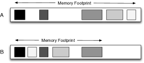
Figure 1: Moving previously allocated blocks into holes left by deallocations can reduce the footprint of the data in storage.

Storage reallocation

This paper generalizes memory allocation by allowing the allocator to move previously allocated objects. We call this generalization storage reallocation. Storage reallocation can take place on any physical medium for allocating objects, e.g., main memory, rotating disks, or flash memory. See Figure 1.

Thus, garbage collection [Jones et al. (2011)] is a type of in-core storage reallocation. More generally, systems that introduce a layer of indirection between logical addresses and physical addresses, such as virtual memory, make reallocation transparent to processes that request storage.

Our own interest in memory reallocation stems from our experience in building the TokuDB [Percona, Inc. (2016a)] and TokuMX [Percona, Inc. (2016b)] databases, in which memory segments are accessed via a so-called “block translation layer,” which translates between the block name, which is immutable, and the block address in storage, which may change. (While TokuDB often reallocates storage, its reallocator does not enjoy the extra property of cost-oblivousness addressed in this paper.)

Cost-oblivious storage reallocation

An algorithm for storage reallocation must contend with the tradeoff between storage footprint size and the amount (and cost) of reallocation. It should come as no surprise that a storage reallocator that is designed for main memory is unlikely to work well if the objects are allocated on a rotating device instead—and vice versa. This is because the cost model depends on where the objects are stored.

The question is therefore how to model the cost of reallocating memory objects. Faithful cost models are hard to come by, in part because the memory hierarchy has a hard-to-quantify impact on run time. In RAM, moving an object is roughly proportional to the object size. On disk, moving a small object may be dominated by the seek time, while moving a large object may be dominated by the disk bandwidth. In both cases, there are cache effects, both in memory and in storage and in their interaction. The performance characteristics for each aspect of memory vary by brand and model.

Rather than model these complex interactions, this paper specifies a class of cost functions that subsumes them. We give universal reallocators, independent of the particulars of the reallocation cost. We say that a universal reallocator is cost oblivious with respect to a class of cost functions if its execution does not depend on the specific choice of cost function from the class. Our reallocation algorithms are cost oblivious with respect to the class of cost functions that are subadditive, monotonically increasing functions of the object size. (A (monotonically increasing) function $f(x)$ is subadditive, if $f(x+y)\leq f(x)+f(y)$ for any positive $x$ and $y$. Note that all monotonically increasing concave functions are subadditive.) The restriction to subadditivity is not severe. While there exist corner cases where a storage system is temporarily superadditive, most mechanisms employed by operating systems, such as prefetching for latency hiding, rely on the subadditivity of costs.

To summarize, in storage reallocation, there is an online sequence of insert (memory allocation, i.e., function malloc) and delete (memory release, i.e., function free) requests. Objects are allocated to locations in an arbitrarily large array (address space). The cost of allocating or moving (reallocating) a size-$w$ object is some unknown (monotonically increasing) subadditive function $f(w)$.

Storage reallocation is thus a bicriteria optimization problem. The first objective is to store objects in an array so that the largest allocated memory address—which we call the footprint—is approximately minimized. The second objective is to minimize the amortized reallocation cost per new request. In this paper, we consider the problem of minimizing the amortized reallocation cost, while using a memory footprint that is at most a constant factor larger than optimal.

Storage reallocation in a database

Databases have many moving parts, and any system that changes the way that storage is allocated needs to interact gracefully with the other requirements of the storage system.

A common constraint in storage (re)allocation is that updates be nonoverlapping, i.e., when an object is moved, its new location must be disjoint from its old location. In databases, object writes are not atomic, so nonoverlapping reallocation is necessary for durability. This is also relevant in other contexts: In SSDs, the nonoverlapping constraint is enforced by the hardware, because memory locations must be erased between writes. In FPGAs, satisfying this constraint allows interruption-free reallocations of modules [Fekete et al. (2012)].

The nonoverlapping constraint is only part of the mechanism for durability. Another consideration is that when an object is moved, the translation table between logical and physical addresses needs to be updated. It is then written to disk during a checkpoint. Only then are blocks that have been freed since the last checkpoint available for reuse. Therefore, the allocator may not write to a location that has been freed after the last checkpoint.

Finally, new memory requests arrive at unpredictable times. It is undesirable for an allocation request to block on a long sequence of reallocations, even if the average throughput is high. A good reallocation algorithm should provide some guarantee on the worst-case cost of individual operations, while still maintaining (near) optimal throughput.

Formalization

An online execution is a sequence of requests of the form ${\left\langle\mbox{{InsertObject}},\mbox{{name}},\mbox{{length}}\right\rangle}$ and ${\left\langle\mbox{{DeleteObject}},\mbox{{name}}\right\rangle}$. After each request, the reallocator outputs an allocation for the objects in the system. We say that an object is active at time $t$ if it has been inserted by one of the first $t$ requests, but not deleted by the end of request $t$. (Note that an object being deleted remains active until the reallocator completes the delete request.)

If $\cal S$ and $\cal S^{\prime}$ are the allocations immediately before and after request $p$, then the reallocation cost of $p$ is the sum of the reallocation costs of all objects moved between $\cal S$ and $\cal S^{\prime}$.

A reallocator $A$ is $(f,a,b)$-competitive for cost function $f()$, if (1) the footprint size is always optimized to within an $a$-factor of optimal, and (2) the reallocation cost is at most $b$ times the sum of the allocation costs of every object inserted so far (including those that have subsequently been deleted). Since every object must be allocated at least once, the cost of such a reallocator is within a factor of $b$ of optimal.

Let $\cal C$ be a set of cost functions. A reallocation algorithm $A$ is cost oblivious if it does not depend on $f()$. This means not only that $f()$ is not a parameter to algorithm $A$, but also $A$ learns nothing about $f()$ as $A$ executes. A cost-oblivious reallocator $A$ is $({\cal C},a,b)$-competitive if it is $(f,a,b)$-competitive for every $f\in{\cal C}$; we abbreviate to $(a,b)$-competitive if the set $\cal C$ is unambiguous. In the remainder of this paper, we take ${\cal C}=\mbox{${\cal F}_{sa}$}$, the class of monotonically increasing, subadditive functions.

Results

Our reallocation algorithms are tunable to achieve an arbitrarily good competitive ratio $1+\varepsilon$ ($0<\varepsilon\leq 1/2$) with respect to the footprint size. All objects have integral length, and $\Delta$ denotes the length of the longest object. We establish the following:

• We give a cost-oblivious algorithm for storage reallocation that is $(\mbox{${\cal F}_{sa}$},1+\varepsilon,O((1/\varepsilon)\log(1/\varepsilon))$-competitive. This allocator is amortized in the sense that it might reallocate every existing object between servicing two requests.

• As a corollary, we give a defragmenter that is cost oblivious with respect to ${\cal F}_{sa}$. The defragmenter takes as input a comparison function, a set of objects having total length $V$ and consuming space $(1+\varepsilon)V$. The defragmenter sorts the objects using $(1+\varepsilon)V+\Delta$ working space, moving each object $O((1/\varepsilon)\log(1/\varepsilon))$ times, amortized.

• We extend the storage reallocator to support checkpointing. With an additional $O(\Delta)$ space, we guarantee that each operation completes within $O(1/\varepsilon)$ checkpoints.

• We also partially deamortize the storage reallocator so that the worst-case reallocation cost (and therefore the worst-case time blocking for a new size-$w$ allocation) is reduced to $O((1/\varepsilon)wf(1)+f(\Delta))$.

There is a variety of possible extensions to this concept. One such direction is to consider the sum of allocation costs; we address this in a related followup paper [Bender et al. (2015)].

Related work

We now review the related work.

Dynamic memory allocation. There is an extensive literature on memory allocation [Knuth (1997), Robson (1971), Robson (1974), Robson (1977), Luby et al. (1996), Naor et al. (2000), Woodall (1974)] where object reallocation is disallowed. There are upper and lower bounds on the competitive ratio of the memory footprint that are roughly logarithmic in the number of requests and in the ratio of the largest to smallest request. These papers generally analyze traditional strategies such as Best Fit, First Fit, and the Buddy System [Knowlton (1965)], but also propose alternatives. Traditional memory-allocation strategies often have analogs in bin-packing [Coffman, Jr. et al. (1983), Coffman, Jr. et al. (1993), Coffman, Jr. et al. (1997), Coffman, Jr. et al. (1997), Galambos and Woeginger (1995)], but an enumeration of such results lies beyond the scope of this paper.

Memory allocation where reallocation is allowed appears often in the literature on garbage collection [Jones et al. (2011)]. There is a long and important line of literature studying dynamic memory allocation with differing compaction mechanisms, exploring the time/space trade-off between the amount of compaction performed and the total memory used. Ting [Ting (1976)] develops a mathematical model for examining this trade-off for different compaction algorithms; Błażewicz et al. [Błażewicz and Nawrocki (1985)] develop a “partial” compaction algorithm for segments of two different sizes that reallocates only a limited number of segments per compaction. More recently Bendersky and Petrank [Bendersky and Petrank (2012)] and Cohen and Petrank [Cohen and Petrank (2013)] have more fully explored the trade-offs inherent in partial compaction.

These papers on dynamic memory allocation with compaction are instances of storage reallocation, as addressed in this paper, where the reallocation cost is (typically) linear: the cost of compaction is directly proportional to the amount of memory that is moved. (These papers often address other problems that arise in garbage collection, such as how to update pointers to memory that has moved.) For example, Bendersky and Petrank [Bendersky and Petrank (2012)] show that when the cost function is linear, one can achieve constant amortized reallocation cost with memory size that is within a constant-factor of optimal.

In this paper, by contrast, we focus on cost-oblivious algorithms that tolerate the range of cost functions found in external storage systems. Cost obliviousness bears a passing resemblance to similar notions in the memory hierarchy, particularly the cache-oblivious/ideal-cache [Frigo et al. (1999), Prokop (1999)], hierarchical memory [Aggarwal et al. (1987)], and cache-adaptive [Bender et al. (2014), Bender et al. (2016)] models. With the exception of the underlying paging [Sleator and Tarjan (1985)], work in these models is about writing algorithms that are memory-hierarchy universal rather than analyzing resource allocation. Although we consider an online setting, even finding optimal offline algorithms seems nontrivial.

Other related work. Storage reallocation has other applications besides databases. For example, Fekete et al. [Fekete et al. (2012)] address the storage reallocation problem in the context of FPGAs, and Bender et al. [Bender et al. (2009)] give (not cost-oblivious) algorithms for constant reallocation cost.

Sparse table data structures [Itai et al. (1981), Willard (1982), Willard (1986), Willard (1992), Katriel (2002), Bender et al. (2005), Itai and Katriel (2007), Bender et al. (2002), Bulánek et al. (2012), Bender and Hu (2007), Bender and Hu (2006), Bender et al. (2016), Bender et al. (2016), Bender et al. (2006), Bender et al. (2017)] also solve the storage reallocation problem and are easily adapted to deal with different-sized objects and linear reallocation cost. But they do so while maintaining the constraint that the object order does not change, which makes the problem harder and the reallocation cost correspondingly larger.

Scheduling/planning interpretation. The storage reallocation problem can be viewed as a reallocation problem in scheduling/planning. In this interpretation, we have an online sequence of requests to insert a new job $j$ into the schedule or to delete an exiting job $j$. Each job has a length $w_{j}$ and the rescheduling cost is $f(w_{j})$. The goal is to maintain a uniprocessor schedule that (approximately) minimizes the makespan (latest completion time of any job), while simultaneously guaranteeing the overall reallocation cost is approximately minimized. We can abbreviate this scheduling problem as $1|f(w)\mbox{\it~{}realloc }|C_{\rm max}$, generalizing standard scheduling notation [Graham et al. (1979)]. The goal is actually not to run the schedule, but rather to plan a schedule subject to an online sequence of changes to the scheduling instance.

We thus review related work in scheduling and combinatorial optimization. Several papers explore related notions of scheduling reallocation (although to the best of our knowledge, not cost-universal scheduling reallocation). Bender et al. [Bender et al. (2013)] study reallocation scheduling with unit-length jobs having release times and deadlines. Their reallocator maintains a feasible multiprocessor schedule while servicing inserts and deletes.

In the area of robust optimization, the goal is to develop solutions for combinatorial optimization problems that are (near) optimal, and that can be readily updated if the instance changes. In this context, many papers have looked at the problem of minimizing reallocation costs for specific optimization problems (e.g., [Hall and Potts (2004), Tamer Unal et al. (1997), Fekete et al. (2012)]). For example, Davis et al. [Davis et al. (2006)] study a reallocation problem, where an allocator divides resources among a set of users, updating the allocation as the users’ constraints change. The goal is to minimize the number of changes to the allocation. As another example, Sanders et al. [Sanders et al. (2009)] look at the problem of assigning jobs to processors, minimizing the reallocation as new jobs arrive. Jansen et al. [Jansen and Klein (2013)] look at robust algorithms for online bin packing that minimize migration costs. See Verschae [Verschae (2012)] for more details on robust optimization.

Shachnai et al. [Shachnai et al. (2012)] explore a slightly different notion of reallocation for combinatorial problems. Given an input, an optimal solution for that input, and a modified version of the input, they develop algorithms that find the minimum-cost modification of the optimal solution to the modified input. A difference between their setting and ours is that we measure the ratio of reallocation cost to allocation cost, whereas they measure the ratio of the actual transition cost to the optimal transition cost resulting in a good solution. Also, we focus on a sequence of changes, which means we amortize the expensive changes against a sequence of updates.

There also exist reoptimization problems, which address the goal of minimizing the computational cost for incrementally updating the schedule [Ausiello et al. (2011), Archetti et al. (2010), Ausiello et al. (2009), Archetti et al. (2003), Böckenhauer et al. (2006)]. By contrast, in reallocation, we focus on the cost of reallocating resources rather than the computational cost of generating the allocation.

2 Footprint Minimization

In this section we give a cost-oblivious algorithm for footprint minimization in storage reallocation. The footprint always has size at most $(1+\varepsilon)V_{t}$, where $V_{t}$ denotes the volume, or total size, of all allocated objects at time $t$, i.e., of the active objects after the $t$th operation completes. A size-$w$ object has an amortized reallocation cost of $O\left(f(w)\cdot(1/\varepsilon)\log(1/\varepsilon)\right)$, where $f(w)$ is the (unknown) cost for allocating an object of size $w$.

Theorem 2.1.

For any constant $\varepsilon$ with $0<\varepsilon\leq 1/2$, there exists a cost-oblivious storage-reallocation algorithm that is $\left(1+\varepsilon,\,O\left((1/\varepsilon)\log(1/\varepsilon)\right)\right)$-competitive with respect to ${\cal F}_{sa}$, the class of monotonically increasing, subadditive cost functions.

Thus, the storage reallocation algorithm is within a constant factor of optimal for any constant $\varepsilon<1/2$.

Intuition and cost-function-specific algorithms

We begin by considering some simple cases where the cost function is known in advance. First suppose that the reallocation cost is linear in the object size, i.e., $f(w)=w$. A simple logging-and-compressing strategy attains a $(2,2)$-competitive algorithm for linear cost functions. Specifically, allocate objects from left to right. Upon a deletion, leave a hole where the object used to be. Whenever a deallocation causes the footprint to reach $2V_{t}$, remove all holes by compacting. The cost to reallocate the entire volume $V_{t}$ is paid for by the $V_{t}$’s worth of elements that were deallocated since the last compaction.

Logging and compressing does not work well for constant reallocation cost, i.e., $f(w)=1$. To see why, suppose the deleted objects have size $\Delta$, and the reallocated elements have size $1$. We may need to spend amortized $\Theta(\Delta)$ reallocation cost per deletion.

There do exist good reallocators for constant reallocation cost [Bender et al. (2009)]. Conceptually, round the object sizes up to the next power of $2$ to form

Definition 1.

size classes, where objects have size $2^{i}$ for $i=0,\ldots,\log{\Delta}$. Now group the objects by increasing size. Between the $i$th and $(i+1)$st size class, there is either a gap of size $2^{i}$ or no gap. To insert an object of size $2^{i}$, put the object into the gap after the $i$th size class, if one exists, or displace a larger object to make space, otherwise. Then recursively reinsert the larger object. The amortized reallocation cost is $O(1)$, because the costs per unit volume to displace the recursively larger objects form a geometric series.

It can be shown, however, that with linear reallocation cost this strategy is only $(2,{\color[rgb]{0,0,0}{\Theta}}(\log\Delta))$-competitive.

This section gives a single algorithm that works for $f(w)=w$, $f(w)=1$, and all other subadditive cost functions. The algorithm keeps the objects partially sorted by size. Since the cost function is subadditive, small objects are the most expensive to move per unit size. We therefore want to guarantee that when an object is inserted or deleted, it can only trigger the movement of larger (less expensive per unit size) objects. Specifically, small objects with total volume $W$ will be able to cause the movements of big objects with total volume $O(W)$, but not the other way around. At the same time, we need to avoid cascading reinserts, which can happen with the algorithm for unit cost described above.

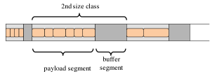
Figure 2: The layout of the data structure when the buffer segments are empty, with $\varepsilon^{\prime}=1/2$. The light-gray are the payload segments, and the dark-gray areas are the buffer segments. The orange rectangles are objects currently in the data structure.

Overview and invariants

Objects are categorized into

Definition 2.

size classes; the $i$th size class contains objects of size $w$, where $2^{i-1}\leq w<2^{i}$. Thus, there are $\left\lfloor\log\Delta\right\rfloor+1$

Definition 3.

size classes. The value of $\Delta$ need not be known in advance. For size class $i$, $V_{t}(i)$ denotes the

Definition 4.

volume (total size) of all objects active at time $t$ in size class $i$. If $t$ is understood, we use $V(i)$.

Intuitively, these size classes allow us to order objects by approximate size, which helps make efficient deletes possible. To maintain our target makespan, we need to reallocate an object when too many objects to its left are deleted. If objects to the right are small and objects to the left are large, then reallocations are too expensive for most cost functions. Within a size class, the ordering does not matter, since it only affects the reallocation cost by a constant factor. We next explain that, in fact, we can even further relax our ordering.

The array (address space) is divided into $\left\lfloor\log\Delta\right\rfloor+1$ regions, as illustrated in Figure 2. The $i$th region is dedicated to the $i$th size class and comprises two subregions, a

Definition 5.

payload segment followed by a

Definition 6.

buffer segment. The $i$th payload segment contains only objects belonging to the $i$th size class, whereas the $i$th buffer segment may contain objects that are in the $i$th size class or smaller size classes.

Whenever (potentially large) reallocations are taking place, an

Definition 7.

overflow segment is used for temporarily rearranging the objects, as described later. The overflow segment is placed at the end of the array.

Invariant 2.2

The following properties are maintained throughout the execution of the algorithm:

1. The $i$th region ($i=1,\ldots,\left\lfloor\log\Delta\right\rfloor+1$) comprises the $i$th payload and $i$th buffer segment.

2. The $(\left\lfloor\log\Delta\right\rfloor+2)$nd region, the overflow segment, stores elements temporarily during reallocation.

3. The $i$th payload segment only stores elements from the $i$th size class.

4. The $i$th buffer segment only stores elements from size classes $\ell\leq i$.

Allocating and deallocating

When a new size-$w$ object that belongs to a size class $i$ is allocated, it is stored at the end of the earliest buffer $j\geq i$ that has sufficient unoccupied space. (Recall that this object cannot be inserted into any buffer in a segment less than $i$.)

When there is not enough available space in any of these buffers, a

Definition 8.

buffer flush operation is triggered (see Figure 3), after which the object is inserted. During a buffer flush, all objects in some suffix of buffers get moved to their proper payload segments and the segment and region boundaries get redefined.

If the new size-$w$ object belongs to a larger size class than any other active object, then we instead create a new payload segment and buffer segment for the new size class located immediately after the last size class’s segment, increasing the total space used by at most an additive $w+\varepsilon^{\prime}w$, for some constant $\varepsilon^{\prime}$. (The overflow segment is empty, because it is only used during a buffer flush, and hence implicitly resides after the new size class.)

When a size-$w$ object is deleted, it leaves a hole until the next buffer flush occurs. A dummy deletion request is added to the buffer and forced to consume $w$ space. This buffered dummy request is not freed until the next buffer flush. Since both inserting and deleting a job of size $w$ reduces the space in the buffer by $w$, we can analyze insertions and deletions together.

Invariant 2.3

The overflow segment is empty except during buffer flush operations.

Invariant 2.4

When a flush of the $i$th buffer segment occurs at time $t$, the object and segment boundaries move so that:

1. the space occupied by the $i$th payload segment after the buffer flush completes is exactly $V_{t}(i)$, and

2. the space occupied by the $i$th buffer segment after the buffer flush completes is $\left\lfloor\varepsilon^{\prime}V_{t}(i)\right\rfloor$, for $\varepsilon^{\prime}=\Theta(\varepsilon)$.

Immediately following this flush, the size-$\left\lfloor\varepsilon^{\prime}V_{t}(i)\right\rfloor$ buffer contains no objects.

As described in this section, $V_{t}(i)$ immediately increases to count the new object, but the object is not yet placed in the array. Next, the flush occurs, and finally the new object is placed in the array. Our extension in Section 3 places the object before performing the flush; this extension requires an additive $\Delta$ working space during the flush procedure.

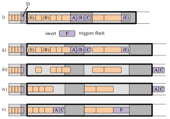
Figure 3: Example of a flush, starting from Figure 2. The lavender rectangles are updates to the data structure, with parentheses and light shading denoting a delete or delete record. (i) The state after insert A, delete B, insert C, insert D, and delete E in that order. (ii)–(v) show a flush that occurs when inserting F. The heavy outline shows the region affected by the flush, i.e., size classes 2 and 3. (ii) The new boundaries for the 2nd and 3rd size class. (iii) The state after moving buffered objects out of the way and dropping deleted objects. (iv) The state after rearranging the payload segments. (v) The state after putting all buffered objects to their proper locations. Observe that for the flushed classes, the buffers are now empty.

Buffer flush

A buffer flush updates the segment boundaries in a suffix of regions, moving all objects to their proper payload segments, and leaving all buffer segments empty to accommodate future insertions.

To execute a buffer flush, first determine the

Definition 9.

boundary size class $b$ and then flush all buffers for size classes $i\geq b$. The value $b$ is defined as the maximum value such that all objects in buffers $i\geq b$ and the object being inserted/deleted belong to size classes at least $b$. To determine $b$, iterate from the largest to the smallest region, examining every object in the region’s buffer. If any object belongs to a size class $s<b$, then update $b$ with the size class $s$. This continues until reaching a size class $b$, where no object from a smaller size class has been encountered.

To flush the size classes $i\geq b$ at time $t$, first calculate $V_{t}(i)$ for all $i\geq b$. The goal is to redistribute these size classes to take space at most $S=(1+\varepsilon^{\prime})\sum_{i\geq b}V_{t}(i)$, i.e., space $V_{t}(i)$ for the $i$th payload segment and $\left\lfloor\varepsilon^{\prime}V_{t}(i)\right\rfloor$ for the $i$th buffer, while moving all objects from buffers into payload segments.

A flush can be implemented to include at most two moves per object in the flushed size classes.

1. First, identify the new array suffix of size $S$ to accommodate payload and buffer segments. Temporarily move all objects from buffer segments to empty space immediately after this suffix (or after the current suffix, if the current suffix is longer due to deletes), removing any dummy delete records from buffers. These objects make up the overflow segment. This first step increases space usage by at most $\sum_{i\geq b}\varepsilon^{\prime}V_{t}(i)$.

2. Next, iterate over payload segments from smallest to largest, moving objects as early as possible, thus removing any gaps left by deleted objects or emptied buffers. At the end of this step, all the objects are packed as far left as possible with no gaps, beginning at the start of region $b$.

3. Then, iterate over payload segments from largest to smallest, moving each object to its final destination in the redistributed array (which is no earlier than its current location). The final destination can be determined by looking at the values $\left\{V_{t}(i)\right\}$; this step reintroduces gaps to accommodate any not-yet-placed objects in the overflow segment and the empty size-$\left\lfloor\varepsilon^{\prime}V_{t}(i)\right\rfloor$ buffers.

4. Finally, iterate over all objects in the overflow segment, placing them in their final destinations at the end of the appropriate payload segments.

Analysis

The proof of Theorem 2.1 follows from Lemmas 2.5 and 2.7 given below, by fixing $\varepsilon^{\prime}=\Theta(\varepsilon)$ appropriately. Lemma 2.5 states that the space used is $1+O(\varepsilon^{\prime})$ times the optimal space usage. Lemma 2.7 states that the reallocation cost is no worse than $O((1/\varepsilon^{\prime})\log(1/\varepsilon^{\prime}))$ times the optimal reallocation cost.

Lemma 2.5.

After processing the first $t$ allocation/deallocation requests, the space used by the storage-reallocation algorithm is $(1+O(\varepsilon^{\prime}))V$, where $V=\sum_{i}V_{t}(i)$.

Proof 2.6.

Let $f_{i}\leq t$ be the previous time the $i$th buffer was flushed. The space used by the buffers and payload segments is at most $(1+\varepsilon^{\prime})\sum_{i}V_{f_{i}}(i)$ by construction, and it may grow to $(1+O(\varepsilon^{\prime}))\sum_{i}V_{f_{i}}(i)$ during the present buffer flush.

To prove the lemma, we need only bound the difference between $\sum_{i}V_{f_{i}}(i)$ and $\sum_{i}V_{t}(i)$. The difference is accounted for by those objects in buffers (including delete records), which amount to at most an $\varepsilon^{\prime}\sum_{i}V_{f_{i}}(i)$ total volume of objects. Thus, we have $\left|\sum_{i}V_{t}(i)-\sum_{i}V_{f_{i}}(i)\right|\leq\varepsilon^{\prime}\sum_{i}V_{f_{i}}(i)$.

The worst-case-ratio overhead occurs when all buffered objects are deletions, in which case $\sum_{i}V_{t}(i)\geq(1-\varepsilon^{\prime})\sum_{i}V_{f_{i}}(i)$.

Thus, at most $(1+O(\varepsilon^{\prime}))\sum_{i}V_{f_{i}}(i)$ space stores at least $(1-\varepsilon^{\prime})\sum_{i}V_{f_{i}}(i)$ active objects. Observing that $(1+O(\varepsilon^{\prime}))/(1-\varepsilon^{\prime})=1+O(\varepsilon^{\prime})$ for $\varepsilon^{\prime}\leq 1/2$ completes the proof.

Lemma 2.7.

For monotonically increasing, subadditive cost functions $f$, the amortized cost of inserting or deleting an object of size $w$ is $O\left(f(w)\cdot(1/\varepsilon)\log(1/\varepsilon)\right)$.

Proof 2.8.

Consider a buffer-flush operation, and let $b$ be the boundary size class (i.e., all size classes $i\geq b$ have their buffers flushed). There are two cases:

Case 1: The $i$th buffer contains $\Omega(\varepsilon^{\prime}V(i))$ volume of objects, for concreteness, say at least $\varepsilon^{\prime}V(i)/2$ volume.

Case 2: The $i$th buffer is

Corollary: Defragmenting/Sorting

A corollary of cost-oblivious storage reallocation is a cost-oblivious defragmentation algorithm, i.e., a cost-oblivious algorithm for sorting the objects while simultaneously respecting constraints on the space usage.

We first compare with naïve defragmentation. If $2V$ working space is allowed, then defragmentation is trivial with two movements per object. First pack the objects into the rightmost $V$ space, using one move per object. Then place each object directly in its final destination within the leftmost $V$ region of space.

The following theorem shows that defragmentation is possible even using $(1+\varepsilon)V+\Delta$ space by applying cost-oblivious storage reallocation as a black box.

Theorem 2.9.

For any $0<\varepsilon\leq 1/2$ there exists a cost-oblivious defragmentation algorithm that takes as input (1) an arbitrary comparison function, (2) a set of objects with volume $V$, and (3) a current allocation of the objects using space at most $(1+\varepsilon)V$. The algorithm sorts the objects according to the comparison function, subject to:

• the total space usage at any time never exceeds $(1+\varepsilon)V+\Delta$ space, and

• the total cost is at most $O((1/\varepsilon)\log(1/\varepsilon))$ times the cost to allocate all of the objects.

Proof 2.10.

First crunch the objects into the rightmost $V$ space, leaving a size-$\left\lfloor\varepsilon V\right\rfloor$ prefix of the array empty. We reserve this prefix to run the cost-universal storage-reallocation algorithm. Starting with the leftmost object in the suffix, remove it from the suffix, store it temporarily in the $\Delta$ additional space, and then insert it into the prefix using cost-universal storage reallocation. Since the storage reallocation guarantees at most $(1+\varepsilon)W$ space usage, for $W$ total volume of objects in the prefix, at no point does the prefix of size at most $(1+\varepsilon)W$ overlap the suffix of size $(V-W)$. When this process completes, the suffix is empty and all objects are in the cost-universal-storage data structure.

Next, move elements back to the suffix in reverse sorted order. Specifically, delete each object from the prefix (using the cost-universal storage-reallocation algorithm), which compacts the space used, and place the object just before its successor in the suffix. Again, at any time, if $W$ is the remaining volume of objects in the prefix, the prefix uses at most $(1+\varepsilon)W$ space, and the suffix uses exactly $V-W$ space, so the prefix does not overlap the suffix.

Note that the additional $\Delta$ working space is unavoidable when reallocating large objects. To see this, consider a single size-$\Delta$ object. This object cannot be moved unless the target location is not overlapping with the original location. That is, if we have less than $2\Delta$ space to work with, the object can never be moved as every target location overlaps its current location.

3 Footprint Minimization in a Database Context

This section extends the storage-reallocation algorithm to take into account issues that arrise in databases: durability and blocking. To provide durability, we extend the algorithm to work with a checkpointing mechanism. Specifically, we show how to complete a buffer flush in $O(1/\varepsilon)$ checkpoints. During a flush, the memory footprint increases by an additive $\Delta$ term, up to $(1+\varepsilon)V+\Delta$, where $V$ is the total length of all active objects, and $\Delta$ is the length of the longest object. The additive $\Delta$ is unavoidable due to the fact that when a large object is moved, its new location cannot overlap its old location.

To prevent updates from blocking for too long, we present a (partially) deamortized version. The deamortized data structure has the same amortized reallocation cost and memory footprint as the original, but it also has a worst-case reallocation cost of $O((1/\varepsilon)wf(1)+f(\Delta))$ for inserting/deleting a size-$w$ object. That is, on each update, the total length of jobs reallocated is roughly proportional to the size of the object being inserted/deleted. Viewed differently, the deamortized bound shows that the desired footprint bound can be maintained with nonblocking updates, as long as the updates arrive infrequently enough that the previous update has been handled, that is, as long as the previous update of size $w$ is followed by a gap of size $\Omega((1/\varepsilon)wf(1)+f(\Delta))$.

3.1 Overview of the Checkpointing Model

Recall that moving an object updates the map that is maintained between logical and physical addresses. From time to time, and specifically during a checkpoint, this map is written to disk, so that a database that is recovering from a crash has access to the updated map. Suppose an object is reallocated. Then the map must be updated. But if a crash occurs before the next checkpoint, the updated map will not be available to the database on recovery. Therefore, we must maintain two copies of the data—at the old and new locations—until the next checkpoint has completed. Only then is it safe to assume that the database knows, in a durable fashion, the new location of the data.

The consequence for designing a reallocator is that from time to time, the database will perform a checkpoint, and all the space that was freed since the last checkpoint will become available. The requirement that moved data reside in two locations until the next checkpoint means that the system needs an enforcement mechanism. This mechanism guarantees that if our algorithm would like to write to a freed but not checkpointed location it will block. Therefore, a reallocation algorithm is better if it requires fewer checkpoints to compete. For example, if we were to write the data to completely new locations, the algorithm would not block on any checkpoints, because we would not be reusing any space. However, the competitive ratio of the footprint would be at least two. We show below that we can achieve our bound of $(1+\varepsilon)$ competitive ratio while blocking on at most $O(1/\varepsilon)$ checkpoints.

The timing of checkpoints is dependent on many considerations beyond the needs for reallocation, so we assume that checkpoints are initiated by the system, rather than our algorithm. There are other models of checkpointing, such as log-trimming through incremental checkpointing. A complete treatment of checkpointing is beyond the scope of this paper, though it would be interesting to see how different types of checkpointing interact with reallocation.

3.2 Flushing with Checkpoints

The goal of the flush here is identical to that in Section 2, but the implementation details differ to accommodate the checkpointing model. Namely, the space used increases by an additive $\Delta$, and the flush itself proceeds in several rounds with checkpoints in between. Another improvement here is that an inserted element gets inserted before the flush completes, whereas in Section 2 we assumed for simplicity that the insert blocks until the flush completes. The memory footprint at the end of the flush is identical to that of the previous algorithm.

Inserting (allocating) and deleting (deallocating)

Since objects only move during a buffer flush, the insert and delete procedure is almost identical to Section 2. The only difference here is that we insert the object before triggering a flush.

To insert an object, place it in the appropriate buffer segment as before. If there is insufficient space to place the object in any following buffer segment, place it at the end of the last buffer segment (filling and exceeding the buffer capacity) and trigger a flush. When deleting an object, insert a dummy delete request as in Section 2. If this delete request would overflow the last buffer, then trigger the flush without using space for the dummy delete request.

Buffer flush

A flush proceeds as follows. First identify the boundary size class $b$ as before. Recall that the flush proceeds on size classes $i\geq b$. Let $L$ denote the endpoint of the last object before the insert/delete that triggers the flush, i.e., if the total space is $S$ including a newly inserted size-$w$ object, then $L=S-w$. (Note that this detail of subtracting off the newly inserted object is important to obtain a space usage of $(1+\varepsilon)V+\Delta$ throughout the flush rather than $(1+\varepsilon)V+O(\Delta)$.) Let $L^{\prime}$ be the desired memory footprint after the flush, but subtracting off the size of any flush-triggering insert; similar to the procedure for “$S$” discussed in Section 2, $L^{\prime}$ can be calculated by first computing $\sum_{i\geq b}(V_{t}(i)+\left\lfloor\varepsilon^{\prime}V_{t}(i)\right\rfloor)$. That is, if the final data structure should take $S^{\prime}$ space after the flush, then $L^{\prime}=S^{\prime}-w$, where $w$ is the size of the last insert if the flush was triggered by an insert. Let $B$ be the total space occupied by the buffers involved in the flush. Move all objects from buffer segments $i\geq b$ to the end of the array, starting from location $(\max\left\{L,L^{\prime}\right\}+B+\Delta)$. The important observation here is that $L+\Delta$ exceeds the location of the newly inserted object, so none of the target locations overlap any of the current objects. Hence all of these movements can be performed within a single checkpoint. The order in which the buffered objects are moved does not matter. This step of the flush is similar to Section 2, except the starting location is up to $B+\Delta$ slots later in the array.

Next, iterate over payload segments from largest to smallest, moving objects as late as possible in the array ending at location $(\max\left\{L,L^{\prime}\right\}+B+\Delta)$. After this step, flushed payload segments are packed as late as possible before location $(\max\left\{L,L^{\prime}\right\}+B+\Delta)$, and flushed buffer segments (including the newly inserted object) are packed as early as possible after $(\max\left\{L,L^{\prime}\right\}+B+\Delta)$.

This payload-packing step, however, moves objects to locations in the array that may have previously been occupied, which would violate the checkpointing model. Instead, break these movements into phases with checkpoints between each phase. Move as many objects as possible before exceeding $B+\Delta$ volume in each phase. Since the largest object has size $\Delta$, the minimum amount moved is $B+1$. As we shall prove, the movements within a phase do not overlap, and the total number of phases is $O(1/\varepsilon^{\prime})$. Aside from checkpointing, this step differs from the version in Section 2 in that objects are packed later in the array rather than earlier, and hence the movements iterate from largest-to-smallest size class rather than smallest-to-largest. The reason for this change is to take advantage of the $B+\Delta$ working space available at the end of the region.

Next, iterate over payload segments from smallest to largest, moving the objects exactly where they should go in the array. This step, again, may move objects to space that was previously occupied, so we again break it into phases consisting of the next $B+1$ to $B+\Delta$ target locations with a checkpoint following each phase.

Finally, move the buffered elements to their target locations. Since all buffered elements are currently located after $(\max\left\{L,L^{\prime}\right\}+B+\Delta)$, and all target locations are before $L^{\prime}+\Delta$, none of these movements overlap, and they can be performed within a single checkpoint.

Analysis

Note that the number of reallocations is similar to that in Section 2, with the only difference being one reallocation for the flush-triggering item. Hence the reallocation cost of Lemma 2.7 holds for this version of the algorithm. The space used after a flush completes is also identical to Section 2. It remains to prove three facts: 1) the space used during a flush is $(1+O(\varepsilon^{\prime}))V+\Delta$ where $V$ is the total volume of active jobs, 2) the object movements between checkpoints only move objects to nonoverlapping locations, and 3) the number of checkpoints is $O(1/\varepsilon^{\prime})$ per flush.

Lemma 3.1.

While processing any allocation/deallocation request, the total footprint used by the algorithm is at most $(1+O(\varepsilon^{\prime}))V+\Delta$, where $V$ denotes the total volume of all currently active objects.

Proof 3.2.

Let $V_{\scriptsize\mbox{{\rm before}}}$ and $V_{\scriptsize\mbox{{\rm after}}}$ denote the total volume of objects before and after the operation, respectively. Let $S_{\scriptsize\mbox{{\rm before}}}$ and $S_{\scriptsize\mbox{{\rm after}}}$ denote the total space of the data structure before and after the operation, respectively. According to Lemma 2.5, we have $S_{\scriptsize\mbox{{\rm before}}}\leq(1+O(\varepsilon^{\prime}))V_{\scriptsize\mbox{{\rm before}}}$, and $S_{\scriptsize\mbox{{\rm after}}}\leq(1+O(\varepsilon^{\prime}))V_{\scriptsize\mbox{{\rm after}}}$. The question is what happens during the operation, notably during a flush operation.

Suppose the flush is triggered by a size-$w$ insertion. The volume during the flush is thus $V=V_{\scriptsize\mbox{{\rm before}}}+w=V_{\scriptsize\mbox{{\rm after}}}$. The space used to store all buffered objects, including the newly inserted object, is at most $w+B$, where $B$ is the total amount of space devoted to buffers before the flush. Note that since the buffers are sized to less than an $\varepsilon^{\prime}$ fraction of the total space, we have $B\leq\varepsilon^{\prime}S_{\scriptsize\mbox{{\rm before}}}$.
Case 1: $S_{\scriptsize\mbox{{\rm before}}}\geq S_{\scriptsize\mbox{{\rm after}}}$. Then these objects are written at an offset of $(S_{\scriptsize\mbox{{\rm before}}}+B+\Delta)$, meaning that the total space during the flush is at most

Case 2: $S_{\scriptsize\mbox{{\rm before}}}<S_{\scriptsize\mbox{{\rm after}}}$. Then these objects are written at an offset of $(S_{\scriptsize\mbox{{\rm after}}}-w)+B+\Delta$. And the total space during the flush is at most $S_{\scriptsize\mbox{{\rm after}}}+2B+\Delta\leq(1+O(\varepsilon^{\prime}))V_{\scriptsize\mbox{{\rm after}}}+\Delta=(1+O(\varepsilon^{\prime}))V+\Delta$, where the steps follow from analogous steps in Case 1.

In the case of a deletion, the argument is similar, except $w$ becomes 0 in all the expressions, and $V=V_{\scriptsize\mbox{{\rm before}}}$ throughout the flush. That is, the deleted object is considered active until the flush completes.

Lemma 3.3.

During a single phase of object movements between two checkpoints, all object starting locations are disjoint from all object ending locations.

Proof 3.4.

First, consider the payload-packing step, where payload segments are packed to the right. At the start of the $j$th phase, let $\ell_{j}$ denote the last cell occupied by the payload segments that have yet to be packed, and let $r_{j}$ denote the first occupied cell later than $\ell_{j}$. We claim that at the start of each phase $r_{j}\geq\ell_{j}+B+\Delta$, which we shall prove by induction. If true, the claim implies disjointness: if the space between $r_{j}$ and $\ell_{j}$ is at least $B+\Delta$, then we can pack up to $B+\Delta$ volume of jobs in front of $r_{j}$ during the $j$th phase before overlapping the ending position of jobs at $\ell_{j}$.

We prove the claim by induction. The claim holds initially because $\ell_{0}\leq L$, and $r_{0}\geq L+B+\Delta$. For the inductive step, observe that if $X$ volume of objects are moved in phase $j$, then $\ell_{j+1}\leq\ell_{j}-X$, and $r_{j+1}=r_{j}-X$. Combined with the inductive assumption that $r_{j}\geq\ell_{j}+B+\Delta$, we get $r_{j+1}\geq(\ell_{j}+B+\Delta)-X\geq((\ell_{j+1}+X)+B+\Delta)-X=\ell_{j+1}+B+\Delta$.

We next consider the unpacking step, where the payload segments are moved to their final positions. Let $\ell_{j}$ denote the last cell occupied by unpacked payload segments at the start of the $j$th phase of movements, and let $r_{j}$ denote the first cell occupied by the yet-to-be unpacked payload objects. We claim that $\ell_{j}+B+\Delta\leq r_{j}$ (but this time we shall prove it by contradiction). If the claim holds, then we can afford to increase $\ell_{j}$ by $B+\Delta$ in each phase without violating the disjointness.

To prove the claim, suppose for the sake of contradiction that $\ell_{j}>r_{j}-B-\Delta$, and let $X$ be the total volume remaining in the packed region. Then the final position of the last payload segment can end no earlier than $\ell_{j}+X>r_{j}+X-B-\Delta$ after the unpacking, and hence the space desired by these payload segments is at least $L^{\prime}>(r_{j}+X)-B-\Delta$. We also have $r_{j}+X=\max\left\{L^{\prime},L\right\}+B+\Delta$ is the offset at which the buffered objects were moved, which we simplify to $r_{j}+X\geq L^{\prime}+B+\Delta$. Combining these two facts, we get $L^{\prime}>(r_{j}+X)-B-\Delta\geq(L^{\prime}+B+\Delta)-B-\Delta=L^{\prime}$, i.e., $L^{\prime}>L^{\prime}$, which is a contradiction.

Lemma 3.5.

The number of checkpoints occurring during a flush is $O(1/\varepsilon^{\prime})$.

Proof 3.6.

The checkpoints are dominated by the packing and unpacking steps. Let $P(i)$ denote the total space of the $i$th payload segment at the time of the flush, i.e., the volume of jobs that were in this size class the last time a flush occurred. Then the total size of flushed buffers is $B=\sum_{i\geq b}\left\lfloor\varepsilon^{\prime}P(i)\right\rfloor$, and the total space of the region being flushed is $S=\sum_{i\geq b}(P(i)+\left\lfloor\varepsilon^{\prime}P(i)\right\rfloor)$. Since each movement phase does more than $B$ work, showing that $B=\Omega(\varepsilon^{\prime}S)$ would be sufficient. The only difficulty is the floor in the expression, so we shall consider the case of large $P(i)$ and small $P(i)$ separately.

Case 1: sufficiently large $P$. More precisely, suppose $B=\sum_{i\geq b}\left\lfloor\varepsilon^{\prime}P(i)\right\rfloor\geq\sum_{i\geq b}\varepsilon^{\prime}P(i)/2$. Then $B=\Omega(\varepsilon^{\prime}S)$, since $\sum_{i\geq b}P(i)\geq S/2$ for $\varepsilon<1$.

Case 2: small $P$. Suppose $B<\sum_{i\geq b}\varepsilon^{\prime}P(i)/2$. Note that $B=\sum_{i\geq b}\left\lfloor\varepsilon^{\prime}P(i)\right\rfloor\geq\sum_{i\geq b}\varepsilon^{\prime}P(i)-\Theta(\log\Delta)$, since there are only $\Theta(\log\Delta)$ size classes. It follows that $B<\sum_{i\geq b}\varepsilon^{\prime}P(i)/2$ implies $\sum_{i\geq b}\varepsilon^{\prime}P(i)=O(\log\Delta)$, and hence $S=O((1/\varepsilon^{\prime})\log\Delta)$. The algorithm tries to move as many objects as it can until exceeding $B+\Delta$ volume, and hence every consecutive pair of phases moves at least $\Delta/2=\Omega(\log\Delta)=\Omega(\varepsilon^{\prime}S)$ volume.

3.3 Deamortizing the Data Structure

As described so far, the data structure is amortized—the average reallocation cost per update is low, but on some updates every active object may need to be reallocated (i.e., when all size classes are involved in a flush). This section improves the worst-case reallocation cost of a size-$w$ update to $O((1/\varepsilon)wf(1)+f(\Delta))$, without hurting the amortized update cost or the maximum footprint.

Note that the deamortization described here builds on the checkpointing modification, yielding a worst-case $O(1/\varepsilon)$ checkpoints per operation.

Modifications to the algorithm

The main idea of our deamortization is that if a buffer flush performs a total of $X$ reallocations by volume, then this work is spread across the subsequent $\varepsilon^{\prime}X$ updates by volume. The question, however, is where to place new objects that are inserted during a flush. If, for example, an insert could trigger a smaller flush while a larger flush is still ongoing, that would present even more challenges. We tackle these problems by adding two more buffers to the data structure and modifying the flush, which serve to avoid the issue of nested flushes.

Augment the data structure to include one size-$\left\lfloor\varepsilon^{\prime}V_{f}\right\rfloor$ buffer, called the

Definition 11.

tail buffer, following all the size-class segments, where $V_{f}$ is the total volume of all jobs active at the start of the previous buffer flush. The tail buffer is like any other buffer: objects are only placed in the tail buffer if all earlier buffers are too full, and a buffer flush is only triggered once the tail buffer becomes full. The point of the large tail buffer is to enable the flush to complete before triggering another flush.

When a flush is triggered, calculate the desired space and the temporary working space as before; however, the space is slightly larger now due to the $\left\lfloor\varepsilon^{\prime}V\right\rfloor$ space necessary for the tail buffer. We treat all space immediately following the temporary working space as another buffer called the

Case 1: some small-object insertion causes the large object to be reallocated. Then that insert has a reallocation cost of at least $f(\Delta)$. Case 2: the large object does not get reallocated. Then the large object must end before position $(3/2)\Delta$ to achieve the footprint bound, and hence there must be at least $\Delta/2$ small objects appearing after the large one. When deleting the large object, those small objects must move in order to restore the $(3/2)\Delta$ footprint bound. Hence the cost of deleting the large objects is $\Omega(\Delta\cdot f(1))\subset\Omega(f(\Delta))$ for subadditive $f$.

References

- [1]
- Aggarwal et al. (1987) Alok Aggarwal, Bowen Alpern, Ashok K. Chandra, and Marc Snir. 1987. A Model for Hierarchical Memory. In Proc. 19th Annual ACM Symposium on Theory of Computing (STOC). 305–314.
- Archetti et al. (2003) Claudia Archetti, Luca Bertazzi, and Maria Grazia Speranza. 2003. Reoptimizing the Traveling Salesman Problem. Networks 42, 3 (2003), 154–159.
- Archetti et al. (2010) Claudia Archetti, Luca Bertazzi, and M. Grazia Speranza. 2010. Reoptimizing the 0-1 knapsack problem. Disc. Appl. Math. 158, 17 (2010), 1879–1887.
- Ausiello et al. (2011) Giorgio Ausiello, Vincenzo Bonifaci, and Bruno Escoffier. 2011. Complexity and Approximation in Reoptimization. In Computability in Context: Computation and Logic in the Real World, S. Barry Cooper and Andrea Sorbi (Eds.). World Scientific, 101–129.
- Ausiello et al. (2009) Giorgio Ausiello, Bruno Escoffier, Jérôme Monnot, and Vangelis Th. Paschos. 2009. Reoptimization of minimum and maximum traveling salesman’s tours. J. Disc. Alg. 7, 4 (2009), 453–463.
- Bender et al. (2016) Michael A. Bender, Jon Berry, Rob Johnson, Thomas M. Kroeger, Samuel McCauley, Cynthia A. Phillips, Bertrand Simon, Shikha Singh, and David Zage. 2016. Anti-Persistence on Persistent Storage: History-Independent Sparse Tables and Dictionaries. In Proc. 35th ACM Symposium on Principles of Database Systems (PODS). 289–302.
- Bender et al. (2002) Michael A. Bender, Richard Cole, Erik D. Demaine, and Martin Farach-Colton. 2002. Scanning and Traversing: Maintaining Data for Traversals in a Memory Hierarchy. In Proc. 10th European Symposium on Algorithms (ESA). 139–151.
- Bender et al. (2016) Michael A. Bender, Erik D. Demaine, Roozbeh Ebrahimi, Jeremy T. Fineman, Rob Johnson, Andrea Lincoln, Jayson Lynch, and Samuel McCauley. 2016. Cache-Adaptive Analysis. In Proc. 28th ACM Symposium on Parallelism in Algorithms and Architectures (SPAA). 135–144.
- Bender et al. (2005) Michael A. Bender, Erik D. Demaine, and Martin Farach-Colton. 2005. Cache-Oblivious B-Trees. SIAM J. Comp. 35, 2 (2005), 341–358.
- Bender et al. (2014) Michael A. Bender, Roozbeh Ebrahimi, Jeremy T. Fineman, Golnaz Ghasemiesfeh, Rob Johnson, and Samuel McCauley. 2014. Cache-Adaptive Algorithms. In Proc. 25th ACM-SIAM Symposium on Discrete Algorithms (SODA). 958–971.
- Bender et al. (2013) Michael A. Bender, Martin Farach-Colton, Sándor P. Fekete, Jeremy T. Fineman, and Seth Gilbert. 2013. Reallocation Problems in Scheduling. In Proc. 25th ACM Symposium on Parallelism in Algorithms and Architectures (SPAA). 271–279.
- Bender et al. (2014) Michael A. Bender, Martin Farach-Colton, Sándor P. Fekete, Jeremy T. Fineman, and Seth Gilbert. 2014. Cost-oblivious Storage Reallocation. In Proc. 33rd ACM SIGMOD-SIGACT-SIGART Symposium on Principles of Database Systems (PODS). 278–288.
- Bender et al. (2006) Michael A. Bender, Martin Farach-Colton, and Miguel A. Mosteiro. 2006. Insertion Sort is O(n log n). Th. Comp. Syst. 39, 3 (2006), 391–397. Special Issue on FUN ’04.
- Bender et al. (2009) Michael A. Bender, Sándor P. Fekete, Tom Kamphans, and Nils Schweer. 2009. Maintaining Arrays of Contiguous Objects. In Proc. 17th International Symposium on Fundamentals of Computation Theory (FCT). 14–25.
- Bender et al. (2017) Michael A. Bender, Jeremy T. Fineman, Seth Gilbert, Tsvi Kopelowitz, and Pablo Montes. 2017. File Maintenance: When in Doubt, Change the Layout!. In Proc. 28th Annual ACM-SIAM Symposium on Discrete Algorithms (SODA). 1503–1522.
- Bender and Hu (2006) Michael A. Bender and Haodong Hu. 2006. An Adaptive Packed-Memory Array. In Proc. 25th ACM SIGMOD-SIGACT-SIGART Symposium on Principles of Database Systems (PODS). 20–29.
- Bender and Hu (2007) Michael A. Bender and Haodong Hu. 2007. An adaptive packed-memory array. ACM Trans. Database Syst. 32, 4 (Nov. 2007), 26:1–26:43.
- Bender et al. (2015) Michael E. Bender, M. Farach-Colton, Sándor P. Fekete, J. Fineman, and S. Gilbert. 2015. Cost-Oblivious Reallocation for Sum of Completion Times. In 27th ACM Symposium on Parallelism in Algorithms and Architectures (SPAA 2015). 143–154.
- Bendersky and Petrank (2012) Anna Bendersky and Erez Petrank. 2012. Space overhead bounds for dynamic memory management with partial compaction. ACM Trans. Program. Lang. Syst. 34, 3 (2012), 13.
- Błażewicz and Nawrocki (1985) Jacek Błażewicz and Jerzy R. Nawrocki. 1985. Dynamic storage allocation with limited compaction - complexity and some practical implications. Discrete Applied Mathematics 10, 3 (1985), 241 – 253.
- Böckenhauer et al. (2006) Hans-Joachim Böckenhauer, Luca Forlizzi, Juraj Hromkovic, Joachim Kneis, Joachim Kupke, Guido Proietti, and Peter Widmayer. 2006. Reusing Optimal TSP Solutions for Locally Modified Input Instances. In Proc. Fourth IFIP International Conference on Theoretical Computer Science (TCS). 251–270.
- Bulánek et al. (2012) Jan Bulánek, Michal Koucký, and Michael Saks. 2012. Tight lower bounds for the online labeling problem. In Proc. 44th Symposium on Theory of Computing (STOC). 1185–1198.
- Coffman, Jr. et al. (1983) Edward G. Coffman, Jr., M. R. Garey, and David S. Johnson. 1983. Dynamic Bin Packing. SIAM J. Comput. 12, 2 (1983), 227–258.
- Coffman, Jr. et al. (1997) Edward G. Coffman, Jr., M. R. Garey, and D. S. Johnson. 1997. Approximation Algorithms for NP-hard Problems. PWS Publishing Co., Chapter Approximation Algorithms for Bin Packing: A Survey, 46–93.
- Coffman, Jr. et al. (1993) Edward G. Coffman, Jr., David S. Johnson, Peter W. Shor, and Richard R. Weber. 1993. Markov chains, computer proofs, and average-case analysis of best fit bin packing. In Proc. Twenty-Fifth Annual ACM Symposium on Theory of Computing (STOC). 412–421.
- Coffman, Jr. et al. (1997) Edward G. Coffman, Jr., David S. Johnson, Peter W. Shor, and Richard R. Weber. 1997. Bin packing with discrete item sizes, part II: Tight bounds on First Fit. Random Struct. Algorithms 10, 1-2 (1997), 69–101.
- Cohen and Petrank (2013) Nachshon Cohen and Erez Petrank. 2013. Limitations of partial compaction: towards practical bounds. In Proc. ACM SIGPLAN Conference on Programming Language Design and Implementation (PLDI). 309–320.
- Davis et al. (2006) Sashka Davis, Jeff Edmonds, and Russell Impagliazzo. 2006. Online Algorithms to Minimize Resource Reallocations and Network Communication. In Proc. APPROX-RANDOM. 104–115.
- Fekete et al. (2012) Sándor P. Fekete, Tom Kamphans, Nils Schweer, Christopher Tessars, Jan C. van der Veen, Josef Angermeier, Dirk Koch, and Jürgen Teich. 2012. Dynamic Defragmentation of Reconfigurable Devices. ACM Trans. Reconf. Technol. Syst. 5, 2, Article 8 (June 2012), 20 pages.
- Frigo et al. (1999) Matteo Frigo, Charles E. Leiserson, Harald Prokop, and Sridhar Ramachandran. 1999. Cache-Oblivious Algorithms. In Proc. 40th Annual Symposium on Foundations of Computer Science (FOCS). 285–297.
- Galambos and Woeginger (1995) Gábor Galambos and Gerhard J. Woeginger. 1995. On-line bin packing - A restricted survey. Math. Meth. of OR 42, 1 (1995), 25–45.
- Graham et al. (1979) Ronald L. Graham, Eugene L. Lawler, Jan Karel Lenstra, and Alexander H.G. Rinnooy Kan. 1979. Optimization and Approximation in Deterministic Sequencing and Scheduling: a Survey. Ann. Disc. Math. 5 (1979), 287 – 326.
- Hall and Potts (2004) Nicholas G. Hall and Chris N. Potts. 2004. Rescheduling for new orders. Operations Research 52, 3 (2004), 440–453.
- Itai and Katriel (2007) Alon Itai and Irit Katriel. 2007. Canonical density control. Inf. Process. Lett. 104, 6 (2007), 200–204.
- Itai et al. (1981) Alon Itai, Alan G. Konheim, and Michael Rodeh. 1981. A Sparse Table Implementation of Priority Queues. In Proc. International Colloquium on Automata, Languages, and Programming (ICALP). 417–431.
- Jansen and Klein (2013) Klaus Jansen and Kim-Manuel Klein. 2013. A Robust AFPTAS for Online Bin Packing with Polynomial Migration,. In Proc. 40th International Colloquium on Automata, Languages, and Programming (ICALP). 589–600.
- Jones et al. (2011) Richard Jones, Antony Hosking, and Eliot Moss. 2011. The Garbage Collection Handbook: The Art of Automatic Memory Management. Chapman and Hall/CRC.
- Katriel (2002) Irit Katriel. 2002. Implicit Data Structures Based on Local Reorganizations. Master’s thesis. Technion – Isreal Inst. of Tech., Haifa.
- Knowlton (1965) Kenneth C. Knowlton. 1965. A Fast Storage Allocator. Commun. ACM 8, 10 (Oct. 1965), 623–624. http://doi.acm.org/10.1145/365628.365655
- Knuth (1997) Donald E. Knuth. 1997. The Art of Computer Programming: Fundamental Algorithms (third ed.). Vol. 1. Addison-Wesley. 435–425 pages.
- Luby et al. (1996) Michael G. Luby, Joseph (Seffi) Naor, and Ariel Orda. 1996. Tight bounds for dynamic storage allocation. SIAM Journal on Discrete Mathematics 9, 1 (1996), 155–166.
- Naor et al. (2000) Joseph (Seffi) Naor, Ariel Orda, and Yael Petruschka. 2000. Dynamic Storage Allocation with Known Durations. Discrete Applied Mathematics 3 (2000), 203–213.
- Percona, Inc. (2016a) Percona, Inc. 2016a. Percona TokuDB. https://www.percona.com/software/mysql-database/percona-tokudb. (2016). viewed August, 2016.
- Percona, Inc. (2016b) Percona, Inc. 2016b. Percona TokuMX. https://www.percona.com/software/mongo-database/percona-tokumx. (2016). viewed August, 2016.
- Prokop (1999) Harald Prokop. 1999. Cache-Oblivious Algorithms. Master’s thesis. Department of Electrical Engineering and Computer Science, Massachusetts Institute of Technology.
- Robson (1971) John M. Robson. 1971. An Estimate of the Store Size Necessary for Dynamic Storage Allocation. J. ACM 18, 3 (July 1971), 416–423.
- Robson (1974) John M. Robson. 1974. Bounds for Some Functions Concerning Dynamic Storage Allocation. J. ACM 21, 3 (July 1974), 491–499.
- Robson (1977) John M. Robson. 1977. Worst Case Fragmentation of First Fit and Best Fit Storage Allocation Strategies. Comput. J. 20, 3 (1977), 242–244.
- Sanders et al. (2009) Peter Sanders, Naveen Sivadasan, and Martin Skutella. 2009. Online Scheduling with Bounded Migration. Math. Oper. Res. 34, 2 (2009), 481–498.
- Shachnai et al. (2012) Hadas Shachnai, Gal Tamir, and Tami Tamir. 2012. A Theory and Algorithms for Combinatorial Reoptimization. In Proc. 10th Latin American Theoretical INformatics Symposium (LATIN). 618–630.
- Sleator and Tarjan (1985) Daniel D. Sleator and Robert E. Tarjan. 1985. Amortized efficiency of list update and paging rules. Commun. ACM 28, 2 (February 1985), 202–208.
- Tamer Unal et al. (1997) Ali Tamer Unal, Reha Uzsoy, and Ali S. Kiran. 1997. Rescheduling on a single machine with part-type dependent setup times and deadlines. Annals of Operations Research 70, 0 (1997), 93–113.
- Ting (1976) Dennis W. Ting. 1976. Allocation and Compaction - a Mathematical Model for Memory Management. In Proc. ACM SIGMETRICS Conference on Computer Performance Modeling Measurement and Evaluation (SIGMETRICS). 311–317.
- Verschae (2012) José C. Verschae. 2012. The Power of Recourse in Online Optimization Robust Solutions for Scheduling, Matroid and MST Problems The Power of Recourse in Online Optimization: Robust Solutions for Scheduling, Matroid and MST Problems. Ph.D. Dissertation. Technischen Universität Berlin.
- Willard (1982) Dan E. Willard. 1982. Maintaining Dense Sequential Files in a Dynamic Environment (Extended Abstract). In Proc. 14th ACM Symposium on Theory of Computing (STOC). 114–121.
- Willard (1986) Dan E. Willard. 1986. Good Worst-Case Algorithms for Inserting and Deleting Records in Dense Sequential Files. In Proc. ACM SIGMOD International Conference on Management of Data. 251–260.
- Willard (1992) Dan E. Willard. 1992. A Density Control Algorithm for Doing Insertions and Deletions in a Sequentially Ordered File in Good Worst-Case Time. Inf. and Comput. 97, 2 (1992), 150–204.
- Woodall (1974) DR Woodall. 1974. The Bay Restaurant–A linear storage problem. The American Mathematical Monthly 81, 3 (1974), 240–246.