Braiding Operator via Quantum Cluster Algebra

Abstract.

We construct a braiding operator in terms of the quantum dilogarithm function based on the quantum cluster algebra. We show that it is a $q$-deformation of the $\mathsf{R}$-operator for which hyperbolic octahedron is assigned. Also shown is that, by taking $q$ to be a root of unity, our braiding operator reduces to the Kashaev $\mathbf{R}^{\text{K}}$-matrix up to a simple gauge-transformation.

1.  Introduction

It is conjectured [27] that the hyperbolic volume of knot complement is given by

$$\lim_{N\to\infty}\frac{2\pi}{N}\log\left|\langle K\rangle_{N}\right|=\operatorname{Vol}(S^{3}\setminus K),$$ (1.1)

where $\langle K\rangle_{N}$ is the Kashaev invariant of knot $K$. Kashaev constructed the quantum invariant $\langle K\rangle_{N}$ based on the finite-dimensional representation of the quantum dilogarithm [25]. It was later realized that the Kashaev invariant $\langle K\rangle_{N}$ coincides with the $N$-colored Jones polynomial at the $N$-th root of unity [32],

$$\langle K\rangle_{N}=J_{N}(K;q=\mathrm{e}^{2\pi\mathrm{i}/N}),$$ (1.2)

where the $N$-colored Jones polynomial is normalized to be $J_{N}(\text{unknot};q)=1$. More precisely it was shown that Kashaev’s braiding matrix  $\mathbf{R}^{\text{K}}$ as a finite-dimensional representation of the Artin braid group with $n$ strands,

$${B}_{n}=\left\langle\sigma_{1},\sigma_{2},\dots,\sigma_{n-1}~{}\middle|~{}\begin{aligned} &\sigma_{i}\,\sigma_{i+1}\,\sigma_{i}=\sigma_{i+1}\,\sigma_{i}\,\sigma_{i+1},\\ &\sigma_{i}\,\sigma_{j}=\sigma_{j}\,\sigma_{i},\quad\text{for $|i-j|>1$}\end{aligned}\right\rangle,$$ (1.3)

is gauge-equivalent to the $\mathbf{R}^{\text{J}}$-matrix for the $N$-colored Jones polynomial at the root of unity. As the colored Jones polynomial is well-understood in the framework of the quantum group $\mathcal{U}_{q}(s\ell_{2})$ (see, e.g., [30]), the Kashaev invariant $\langle K\rangle_{N}$ is regarded as an invariant for $\mathcal{U}_{\mathrm{e}^{\pi\mathrm{i}/N}}(s\ell_{2})$. In [24, 26, 2] (see also [9]) studied is a relationship between $\langle K\rangle_{N}$ and the $6j$-symbol of $\mathcal{U}_{\mathrm{e}^{\pi\mathrm{i}/N}}(s\ell_{2})$, but the mathematical background of the Kashaev $\mathbf{R}^{\text{K}}$-matrix itself still remains unclear, at least, to us.

Meanwhile, studies on the geometrical content of $\langle K\rangle_{N}$ have been much developed. It is now recognized that an ideal hyperbolic octahedron is assigned to each $\mathbf{R}^{\text{K}}$-matrix [37], and proposed [8, 41] was a method to construct from a set of such octahedra the Neumann–Zagier potential function [34] which give the complex volume of knot complement. This observation is based on a fact that the hyperbolic volume of ideal tetrahedron is given in terms of the dilogarithm function (see, e.g., [38]), and that the $\mathbf{R}^{\text{K}}$-matrix asymptotically consists of four dilogarithm functions [37].

In our previous paper [23], we constructed the $\mathsf{R}$-operator from the viewpoint of the cluster algebra. We showed that the $\mathsf{R}$-operator is geometrically interpreted as a hyperbolic octahedron which is the same assigned to the Kashaev $\mathbf{R}^{\text{K}}$-matrix. The cluster algebra was originally introduced by S. Fomin and A. Zelevinsky [19] to study the total positivity in semi-simple Lie groups, and it is promising to clarify a deep connection with geometry [18] (see also [33, 22]).

The purpose of this article is to quantize the $\mathsf{R}$-operator in [23]. Basic tool is the quantum cluster algebra [6, 31, 17, 16]. We shall construct the $\mathcal{R}$-operator in terms of the quantum dilogarithm function as a conjugation for the quantum $\mathsf{R}^{q}$-operator, and clarify a relationship with the Kashaev $\mathbf{R}^{\text{K}}$-matrix. We show explicitly that the $\mathcal{R}$-operator reduces to the $\mathbf{R}^{\text{K}}$-matrix up to a gauge-transformation when the quantized parameter $q^{2}$ tends to the $N$-th root of unity.

This paper is organized as follows. In Section 2, we briefly review our previous results [22, 23]. We discuss a relationship between the cluster algebra and the hyperbolic geometry, and we recall a definition of the $\mathsf{R}$-operator (2.9) which is illustrated as a hyperbolic octahedron. In Section 3 we study a $q$-deformation of the $\mathsf{R}$-operator. We construct the braiding $\mathsf{R}^{q}$-operator (3.9) as a conjugation of the $\mathcal{R}$-operator (3.15), which is written in terms of the quantum dilogarithm function. In a limit that $q^{2}$ goes to a root of unity, the $\mathcal{R}$-operator reduces to the Kashaev $\mathbf{R}^{\text{K}}$-matrix.

2.  Cluster Algebra and Hyperbolic Geometry

2.1  Cluster Algebra

We briefly collect a notion of the cluster algebra. See [19] for detail.

Fix a positive integer $N$. Let $(\boldsymbol{x},\mathbf{B})$ be a cluster seed, where $\boldsymbol{x}=(x_{1},x_{2},\dots,x_{N})$ is a cluster variable, and an $N\times N$ skew-symmetric integral matrix $\mathbf{B}=(b_{ij})$ is an exchange matrix. The exchange matrix is depicted as a quiver which has $N$ vertices, by regarding

$$b_{ij}=\#\left\{\text{arrows from $i$ to $j$}\right\}-\#\left\{\text{arrows from $j$ to $i$}\right\}.$$ (2.1)

What is important is an operation on cluster seeds, which is called the mutation. For $k=1,\ldots,N$, the mutation $\mu_{k}$ of $(\boldsymbol{x},\mathbf{B})$ is defined by

$$\mu_{k}(\boldsymbol{x},\mathbf{B})=(\widetilde{\boldsymbol{x}},\widetilde{\mathbf{B}}),$$ (2.2)

where a cluster variable $\widetilde{\boldsymbol{x}}=(\widetilde{x}_{1},\dots,\widetilde{x}_{N})$ and an exchange matrix $\widetilde{\mathbf{B}}=(\widetilde{b}_{ij})$ are respectively given by

$$\widetilde{x}_{i}=\begin{cases}x_{i},&\text{for $i\neq k$,}\\[8.61108pt] \displaystyle\frac{1}{x_{k}}\,\left(\prod_{j:b_{jk}>0}x_{j}^{~{}b_{jk}}+\prod_{j:b_{jk}<0}x_{j}^{~{}-b_{jk}}\right),&\text{for $i=k$,}\end{cases}$$ (2.3)

$$\widetilde{b}_{ij}=\begin{cases}-b_{ij},&\text{for $i=k$ or $j=k$},\\[8.61108pt] \displaystyle b_{ij}+\frac{\bigl{|}b_{ik}\bigr{|}\,b_{kj}+b_{ik}\,\bigl{|}b_{kj}\bigr{|}}{2},&\text{otherwise.}\end{cases}$$ (2.4)

In this article, for each seed $(\boldsymbol{x},\mathbf{B})$ we define the $y$-variable $\boldsymbol{y}=(y_{1},\dots,y_{N})$ as

$$y_{j}=\prod_{k}x_{k}^{~{}b_{kj}}.$$ (2.5)

The mutation of the cluster seed induces the mutation of the $y$-variable,

$$\mu_{k}(\boldsymbol{y},\mathbf{B})=(\widetilde{\boldsymbol{y}},\widetilde{\mathbf{B}}),$$ (2.6)

where the exchange matrix $\widetilde{\mathbf{B}}$ is (2.4), and $\widetilde{y}_{j}=\prod_{k}\widetilde{x}_{k}^{~{}\widetilde{b}_{kj}}$ is given by

$$\widetilde{y}_{i}=\begin{cases}y_{k}^{~{}-1},&\text{for $i=k$,}\\[8.61108pt] y_{i}\,\left(1+y_{k}^{~{}-1}\right)^{-b_{ki}},&\text{for $i\neq k$, $b_{ki}\geq 0$,}\\[8.61108pt] y_{i}\left(1+y_{k}\right)^{-b_{ki}},&\text{for $i\neq k$, $b_{ki}\leq 0$.}\end{cases}$$ (2.7)

Figure 1. Quiver for the exchange matrix $\mathbf{B}$ (2.8).

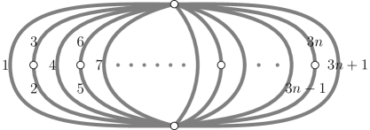
Figure 2. Triangulation of an $(n+2)$-punctured disk. Each edge corresponds to the vertex of the quiver in Fig. 1.

2.2  Braiding Operator

To study the braid group $B_{n}$ (1.3), we set the exchange matrix $\mathbf{B}$ to be a $(3n+1)\times(3n+1)$ skew-symmetric matrix [23]

$$\mathbf{B}=\begin{pmatrix}0&1&-1&0&0&\cdots&\cdots&\cdots&0\\ -1&0&0&1&0&\ddots&\cdots&\cdots&\vdots\\ 1&0&0&-1&0&0&\ddots&\cdots&\vdots\\ 0&-1&1&0&1&-1&0&\ddots&\vdots\\ 0&0&0&-1&0&0&1&\ddots&0\\ \vdots&\ddots&0&1&0&0&-1&\ddots&0\\ \vdots&\vdots&\ddots&0&-1&1&0&\ddots&1\\ \vdots&\vdots&\vdots&\ddots&\ddots&\ddots&\ddots&\ddots&-1\\ 0&\cdots&\cdots&\cdots&0&0&-1&1&0\end{pmatrix}.$$ (2.8)

See Fig. 1 for the associated quiver. We remark that the quiver gives rise to a triangulation of a punctured disk, whose edges correspond to the vertices in the quiver. See Fig. 2. We define the $\mathsf{R}$-operator acting on a cluster seed $(\boldsymbol{x},\mathbf{B})$ by

$$\overset{i}{\mathsf{R}}=s_{3i,3i+2}\,s_{3i-1,3i+2}\,s_{3i,3i+3}\,\mu_{3i+1}\,\mu_{3i-1}\,\mu_{3i+3}\,\mu_{3i+1},$$ (2.9)

for $i=1,\ldots,n-1$, where $s_{i,j}$ is the permutation of subscripts, e.g.,

$$s_{i,j}(\dots,x_{i},\dots,x_{j},\dots)=(\dots,x_{j},\dots,x_{i},\dots).$$

As the exchange matrix $\mathbf{B}$ is invariant under $\overset{i}{\mathsf{R}}$, we write $(\overset{i}{\mathsf{R}}(\boldsymbol{x}),\mathbf{B})$ for $\overset{i}{\mathsf{R}}(\boldsymbol{x},\mathbf{B})$ with

$$\overset{i}{\mathsf{R}}(\boldsymbol{x})=\left(x_{1},\dots,x_{3i-3},\mathsf{R}_{x}(x_{3i-2},\dots,x_{3i+4}),x_{3i+5},\dots,x_{3n+1}\right),$$ (2.10)

where we have from (2.3)

$$\begin{aligned} &\mathsf{R}_{x}(x_{1},x_{2},\dots,x_{7})=\Bigl{(}x_{1},x_{5},\frac{x_{1}\,x_{3}\,x_{5}+x_{3}\,x_{4}\,x_{5}+x_{1}\,x_{2}\,x_{6}}{x_{2}\,x_{4}},\\ &\qquad\frac{x_{1}\,x_{3}\,x_{4}\,x_{5}+x_{3}\,x_{4}^{~{}2}\,x_{5}+x_{1}\ x_{3}\,x_{5}\,x_{7}+x_{3}\,x_{4}\,x_{5}\,x_{7}+x_{1}\,x_{2}\,x_{6}\,x_{7}}{x_{2}\,x_{4}\,x_{6}},\\ &\qquad\qquad\frac{x_{3}\,x_{4}\,x_{5}+x_{3}\,x_{5}\,x_{7}+x_{2}\,x_{6}\,x_{7}}{x_{4}\,x_{6}},x_{3},x_{7}\Bigr{)}.\end{aligned}$$ (2.11)

By definition (2.5), the action on the $y$-variable $\boldsymbol{y}$ is induced as

$$\overset{i}{\mathsf{R}}(\boldsymbol{y})=\left(y_{1},\dots,y_{3i-3},\mathsf{R}_{y}(y_{3i-2},\dots,y_{3i+4}),y_{3i+5},\dots,y_{3n+1}\right),$$ (2.12)

where (2.6) gives

$$\begin{aligned} &\mathsf{R}_{y}(y_{1},y_{2},\dots,y_{7})=\Bigl{(}y_{1}\,\left(1+y_{2}+y_{2}y_{4}\right),\frac{y_{2}\,y_{4}\,y_{5}\,y_{6}}{1+y_{2}+y_{6}+y_{2}\,y_{6}+y_{2}\,y_{4}\,y_{6}},\\ &\qquad\frac{1+y_{2}+y_{6}+y_{2}\,y_{6}+y_{2}\,y_{4}\,y_{6}}{y_{2}\,y_{4}},\frac{y_{4}}{(1+y_{2}+y_{2}\,y_{4})\,(1+y_{6}+y_{4}\,y_{6})},\\ &\qquad\frac{1+y_{2}+y_{6}+y_{2}\,y_{6}+y_{2}\,y_{4}\,y_{6}}{y_{4}\,y_{6}},\frac{y_{2}\,y_{3}\,y_{4}\,y_{6}}{1+y_{2}+y_{6}+y_{2}\,y_{6}+y_{2}\,y_{4}\,y_{6}},\left(1+y_{6}+y_{4}\,y_{6}\right)\,y_{7}\Bigr{)}.\end{aligned}$$ (2.13)

We use $\overset{i}{\mathsf{R}}$ in both (2.10) and (2.12) without confusion.

In [23], it was shown that the $\mathsf{R}$-operator represents the braid group $B_{n}$, and that we have,

$$\overset{i}{\mathsf{R}}\,\overset{i+1}{\mathsf{R}}\,\overset{i}{\mathsf{R}} =\overset{i+1}{\mathsf{R}}\,\overset{i}{\mathsf{R}}\,\overset{i+1}{\mathsf{R}},$$ (2.14)

$$\overset{i}{\mathsf{R}}\,\overset{j}{\mathsf{R}} =\overset{j}{\mathsf{R}}\,\overset{i}{\mathsf{R}},\qquad\text{for $|i-j|>1$.}$$

This can be proved by direct computations using (2.11) and (2.13). We note that the birational Yang–Baxter map in [11] is intrinsically same with (2.11). The braid relation (2.14) could as well be checked from a dual picture as follows. We recall that the mutation is regarded as a “flip” of triangulation of a punctured disk [18]. Here a flip is meant to remove a common edge of two adjacent triangles and to reproduce another different diagonal edge of quadrilateral (see, for example, Fig. 3). This interpretation explains the action of the $\overset{1}{\mathsf{R}}$-operator on a punctured disk as illustrated in Fig. 4. We find that the $\mathsf{R}$-operator on the punctured disk is nothing but a half Dehn twist exchanging two punctures counter-clockwise. This clarification of the braid group is well-known (see, e.g., [7]), and the braid relation (2.14) follows immediately.

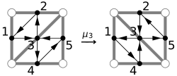
Figure 3. The mutation on a quiver is interpreted as a flip in triangulated punctured surface.

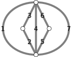
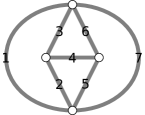
$\xrightarrow[]{\mu_{4}}$	$\xrightarrow[]{\mu_{6}}$
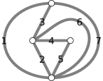
		$\phantom{\mu_{2}}\left\downarrow\rule{0.0pt}{8.53581pt}\right.{\scriptstyle{\mu_{2}}}$
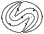
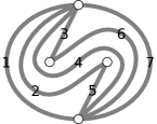
$\xleftarrow[]{s}$	$\xleftarrow[]{\mu_{4}}$

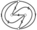
Figure 4. The $\mathsf{R}$-operator as a half Dehn twist. Illustrated is the action of $\overset{1}{\mathsf{R}}=s\,\mu_{4}\mu_{2}\mu_{6}\mu_{4}$ with $s=s_{3,5}s_{2,5}s_{3,6}$ on the punctured disk. One sees that the $\mathsf{R}$-operator is regarded as the half Dehn twist exchanging two punctures counter-clockwise.

A geometrical interpretation of the $\mathsf{R}$-operator is given from the three-dimensional picture of the flip [22]. The mutation in Fig. 3 acts on the $y$-variable as

$$\begin{cases}\widetilde{y}_{1}=y_{1}(1+y_{3}),\\ \widetilde{y}_{2}=y_{2}(1+y_{3}^{-1})^{-1},\\ \widetilde{y}_{3}=y_{3}^{-1},\\ \widetilde{y}_{4}=y_{4}(1+y_{3}^{-1})^{-1},\\ \widetilde{y}_{5}=y_{5}(1+y_{3}).\end{cases}$$

The flip in Fig. 3 is interpreted as a gluing of a hyperbolic ideal tetrahedron to a triangulation of punctured disk as in Fig. 5. Here the ideal hyperbolic tetrahedron has a shape parameter $z$, and a dihedral angle of each edge is parameterized by $z$, $z^{\prime}=1-z^{-1}$, and $z^{\prime\prime}=(1-z)^{-1}$ as in Fig. 6 (see, e.g., [38]). Then each dihedral angle on triangulated surface after the gluing is read as

$$\begin{cases}\widetilde{z}_{1}=z_{1}\,z^{\prime},\\ \widetilde{z}_{2}=z_{2}\,z^{\prime\prime},\\ \widetilde{z}_{3}=z,\\ \widetilde{z}_{4}=z_{4}\,z^{\prime\prime},\\ \widetilde{z}_{5}=z_{5}\,z^{\prime},\end{cases}$$

with a consistency condition $z_{3}\,z=1$. These two sets of equations indicate a correspondence between the $y$-variables and the dihedral angles of triangulated surface, $z_{k}=-y_{k}$, and we conclude that the mutation is regarded as a gluing of an ideal tetrahedron with shape parameter $z=-y_{3}^{-1}$ to punctured surface.

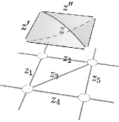
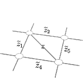
Figure 5. Interpretation of the flip in Fig. 3. A gluing of an ideal tetrahedra to a triangulated surface (left) results in a flipped triangulated surface (right). Here labeled is a dihedral angle of edge. Consistency condition gives $z\,z_{3}=1$, and we have $\widetilde{z}_{1}=z_{1}\,z^{\prime}$ and so on. This transformation is identified with the mutation of $y$-variable in Fig. 3 [22].

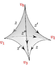
Figure 6. Hyperbolic ideal tetrahedron with a shape parameter $z$. Labeled is a dihedral angle of each edge. Here vertices $v_{a}$ are on the boundary $\partial\mathbb{H}^{3}$, and we mean $z^{\prime}=1-z^{-1}$ and $z^{\prime\prime}=(1-z)^{-1}$. Note that opposite edges have the same dihedral angle.

As a consequence, the cluster $\mathsf{R}$-operator (2.9), which consists of four mutations, can be regarded as an ideal octahedron in Fig. 7. See that every dihedral angle is written in terms of the $y$-variable. Accordingly, the hyperbolic volume of the octahedron for $\widetilde{\boldsymbol{y}}=\overset{i}{\mathsf{R}}(\boldsymbol{y})$ is given by

$$D(-1/y_{3i+1})+D(\widetilde{y}_{3i-2}/y_{3i-2})+D(-\widetilde{y}_{3i+1})+D(\widetilde{y}_{3i+4}/y_{3i+4}),$$ (2.15)

where $D(z)$ is the Bloch–Wigner function (see, e.g., [42]),

$$D(z)=\Im\operatorname{Li_{2}}(z)+\arg(1-z)\,\log|z|.$$

It should be noted that this type of the hyperbolic octahedron is used not only in studies of the Kashaev $\mathbf{R}^{\text{K}}$-matrix [37] but in SnapPea algorithm [39]. Note also that the cluster variable $\boldsymbol{x}$ is identified with Zickert’s edge parameter [43]. See [23] for detail.

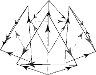
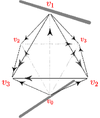
Figure 7. Octahedron assigned to crossing (center). Four oriented tetrahedra (left) are glued together. A dihedral angle of each edge is given in terms of the $y$-variable, and we give dihedral angles around central axis (right). Here we assume $\widetilde{\boldsymbol{y}}=\overset{1}{\mathsf{R}}(\boldsymbol{y})$.

3.  Quantization

3.1  Quantum Cluster Algebra

We recall a quantization of the cluster algebra based on [17, 16]. Fix a parameter $q$. The $y$-variable is quantized to be a $q$-commuting generator $\boldsymbol{Y}=(Y_{1},\ldots,Y_{N})$ satisfying

$$Y_{k}\,Y_{j}=q^{2b_{jk}}Y_{j}\,Y_{k},$$ (3.1)

where $\mathbf{B}=(b_{ij})$ is the skew-symmetric exchange matrix used in the classical cluster algebra. The $q$-commuting relation (3.1) is realized by

$$Y_{k}=\mathrm{e}^{2\pi b\widehat{y}_{k}},$$ (3.2)

where $q=\mathrm{e}^{\pi\mathrm{i}b^{2}}$ and

$$[\widehat{y}_{k}~{},~{}\widehat{y}_{j}]=\frac{\mathrm{i}}{2\pi}b_{jk}.$$ (3.3)

The $q$-deformation of the mutation (2.6) on the $y$-variable is defined by

$$\mu^{q}_{k}(\boldsymbol{Y},\mathbf{B})=(\widetilde{\boldsymbol{Y}},\widetilde{\mathbf{B}}),$$ (3.4)

where the exchange matrix $\widetilde{\mathbf{B}}$ is (2.4), and

$$\widetilde{Y}_{i}=\begin{cases}Y_{k}^{-1},&\text{for $i=k$,}\\[8.61108pt] \displaystyle Y_{i}\,\prod_{m=1}^{b_{ki}}\left(1+q^{2m-1}\,Y_{k}^{-1}\right)^{-1},&\text{for $i\neq k$, $b_{ki}\geq 0$,}\\[8.61108pt] \displaystyle Y_{i}\,\prod_{m=1}^{-b_{ki}}\left(1+q^{2m-1}\,Y_{k}\right),&\text{for $i\neq k$, $b_{ki}\leq 0$.}\end{cases}$$ (3.5)

One sees that this reduces to the classical mutation (2.6) in $q\to 1$.

It is known that the quantum mutation $\mu^{q}_{k}$ (3.4) is decomposed into

$$\mu^{q}_{k}=\mu^{\sharp}_{k}\circ\mu^{\prime}_{k}.$$ (3.6)

Here $\mu^{\prime}_{k}$ is given by

$$Y_{i}\mapsto\begin{cases}Y_{k}^{-1},&\text{for $i=k$,}\\ q^{b_{ik}b_{ki}}\,Y_{i}\,Y_{k}^{b_{ki}},&\text{for $i\neq k$, $b_{ki}\geq 0$,}\\ Y_{i},&\text{for $i\neq k$, $b_{ki}\leq 0$,}\end{cases}$$ (3.7)

and $\mu^{\sharp}_{k}$ is a conjugation by the quantum dilogarithm function

$$\mu^{\sharp}_{k}=\operatorname{Ad}(\Phi(\widehat{y}_{k})):Y_{i}\mapsto\Phi(\widehat{y}_{k})\,Y_{i}\Phi(\widehat{y}_{k})^{-1}.$$ (3.8)

See Appendix A for definition and properties of the quantum dilogarithm function $\Phi(y)$. Note that the quantum mutation $\mu_{k}^{q}$ is not a conjugation in general.

3.2  Braiding Operator

We now consider the quantum cluster algebra for the exchange matrix $\mathbf{B}$ (2.8), whose quiver and dual picture as a triangulation are respectively given in Fig. 1 and Fig. 2.

As a natural quantization of the $\mathsf{R}$-operator (2.9), we define a quantum braiding operator acting on $(\boldsymbol{Y},\mathbf{B})$ by

$$\overset{i\phantom{q}}{\mathsf{R}^{q}}=s_{3i,3i+2}\,s_{3i-1,3i+2}\,s_{3i,3i+3}\,\mu^{q}_{3i+1}\,\mu^{q}_{3i-1}\,\mu^{q}_{3i+3}\,\mu^{q}_{3i+1}.$$ (3.9)

Along with the classical case the exchange matrix $\mathbf{B}$ (2.8) is invariant under the operator $\overset{i\phantom{q}}{\mathsf{R}^{q}}$, and (3.5) gives an action on $\boldsymbol{Y}$ as

$$\overset{i\phantom{q}}{\mathsf{R}^{q}}(\boldsymbol{Y})=\left(Y_{1},\dots,Y_{3i-3},\mathsf{R}_{y}^{q}(Y_{3i-2},\dots,Y_{3i+4}),Y_{3i+5},\dots,Y_{3n+1}\right),$$ (3.10)

where

$$\mathsf{R}_{y}^{q}(Y_{1},\dots,Y_{7})=\begin{pmatrix}Y_{1}(1+qY_{2}^{\prime})\\ Y_{5}(1+qY_{4}^{-1})^{-1}(1+q{Y_{2}^{\prime}}^{-1})^{-1}(1+q{Y_{6}^{\prime}}^{-1})^{-1}(1+q{Y_{4}^{\prime\prime}}^{-1})^{-1}\\ {Y_{2}^{\prime}}^{-1}(1+qY_{4}^{\prime\prime})\\ {Y_{4}^{\prime\prime}}^{-1}\\ {Y_{6}^{\prime}}^{-1}(1+qY_{4}^{\prime\prime})\\ Y_{3}(1+qY_{4}^{-1})^{-1}(1+q{Y_{2}^{\prime}}^{-1})^{-1}(1+q{Y_{6}^{\prime}}^{-1})^{-1}(1+q{Y_{4}^{\prime\prime}}^{-1})^{-1}\\ Y_{7}(1+qY_{6}^{\prime})\end{pmatrix}^{\top}.$$ (3.11)

Here we have used

$$Y_{2}^{\prime}=Y_{2}(1+qY_{4}), Y_{6}^{\prime}=Y_{6}(1+qY_{4}), Y_{4}^{\prime\prime}=Y_{4}^{-1}(1+qY_{2}^{\prime})(1+qY_{6}^{\prime}).$$ (3.12)

Clearly (3.11) reduces to (2.13) when $q\to 1$.

In our noncommutative algebra (3.1) with (2.8), there exist central elements, $Y_{3i-1}Y_{3i}$ ($i=1,\ldots,n$) and $Y_{1}Y_{4}\cdots Y_{3n+1}$. For simplicity we consider a subspace defined by

$$\widehat{y}_{3i-1}+\widehat{y}_{3i}=c,\qquad\text{for }i=1,\ldots,n,$$ (3.13)

where $c\in\mathbb{R}$. In this setting, we find that, in contrast to that $\mu_{k}^{q}$ (3.4) is not an adjoint operator, the $\mathsf{R}^{q}$-operator (3.9) is written as a conjugation

$$\overset{i\phantom{q}}{\mathsf{R}^{q}}(\boldsymbol{Y})=\operatorname{Ad}(\overset{i}{\mathcal{R}})(\boldsymbol{Y})=\overset{i}{\mathcal{R}\vphantom{{}^{-1}}}\,\boldsymbol{Y}\,\overset{i\phantom{-1}}{\mathcal{R}^{-1}},$$ (3.14)

where

$$\overset{i}{\mathcal{R}} =\Phi(\widehat{y}_{3i+1})\,\Phi(\widehat{y}_{3i-1})\,\Phi(\widehat{y}_{3i+3})\,\Phi(\widehat{y}_{3i+1})^{-1}\,\theta(c+\widehat{y}_{3i+1}).$$ (3.15)

See (A.10) for the definition of $\theta(z)$. We can check (3.14) by a direct computation using (A.5). See Appendix B. Furthermore we find that the $\mathcal{R}$-operator (3.15) fulfills the braid relation

$$\overset{i}{\mathcal{R}}\,\overset{i+1}{\mathcal{R}}\,\overset{i}{\mathcal{R}}=\overset{i+1}{\mathcal{R}}\,\overset{i}{\mathcal{R}}\,\overset{i+1}{\mathcal{R}},$$ (3.16)

$$\overset{i}{\mathcal{R}}\,\overset{j}{\mathcal{R}}=\overset{j}{\mathcal{R}}\,\overset{i}{\mathcal{R}},\qquad\text{for $|i-j|>1$.}$$

See Appendix C for the proof. Note that the essentially same solution of the braid relation was studied in [13, 28] .

As we have seen in the previous section that the classical $\mathsf{R}$-operator (2.9) on the $y$-variable is interpreted as an ideal hyperbolic octahedron, the $\mathcal{R}$-operator (3.15) introduced as an adjoint operator for the quantum $\mathsf{R}^{q}$-operator (3.14) should be regarded as a quantum content of the octahedron. It is convincing since the function $\Phi(z)$ reduces, in a classical limit $b\to 0$, to the dilogarithm function (A.6), which is related to the hyperbolic volume of ideal tetrahedron (2.2).

3.3  Braiding Matrix at Generic $q$

We shall give an infinite-dimensional representation of the quantum $\mathcal{R}$-operator (3.15). For this purpose, we set $c=c^{\prime}+c^{\prime\prime}$ and

$$\widehat{y}_{3i-2} =\widehat{x}_{i-1}-\widehat{x}_{i},$$ (3.17)

$$\widehat{y}_{3i-1} =\widehat{p}_{i}+c^{\prime},$$

$$\widehat{y}_{3i} =-\widehat{p}_{i}+c^{\prime\prime},$$

where we mean $\widehat{x}_{0}=\widehat{x}_{n+1}=0$, and $\widehat{x}_{i}$ and $\widehat{p}_{i}$ are generators of the Heisenberg algebra,

$$[\widehat{x}_{i}~{},~{}\widehat{x}_{j}]=[\widehat{p}_{i}~{},~{}\widehat{p}_{j}]=0, [\widehat{x}_{i}~{},~{}\widehat{p}_{j}]=\frac{\mathrm{i}}{2\pi}\delta_{ij}.$$ (3.18)

We define bases in coordinate and momentum spaces, $\left|x\right\rangle$ and $\left|p\right\rangle$, by

$$\widehat{x}_{i}\left|x\right\rangle=x_{i}\left|x\right\rangle, \widehat{p}_{i}\left|p\right\rangle=p_{i}\left|p\right\rangle.$$

These are orthonormal bases satisfying

$$\begin{aligned} &\left\langle x\middle|x^{\prime}\right\rangle=\prod_{i=1}^{n}\delta(x_{i}-x^{\prime}_{i}),&\qquad&\left\langle p\middle|p^{\prime}\right\rangle=\prod_{i=1}^{n}\delta(p_{i}-p^{\prime}_{i}),\end{aligned}$$

$$\left\langle x\middle|p\right\rangle=\overline{\left\langle p\middle|x\right\rangle}=\mathrm{e}^{2\pi\mathrm{i}\sum_{i}x_{i}p_{i}},$$

$$\int\limits_{\mathbb{R}^{n}}\left|x\right\rangle\left\langle x\right|dx=\int\limits_{\mathbb{R}^{n}}\left|p\right\rangle\left\langle p\right|dp=1,$$

A matrix element $\left\langle x\right|\overset{1}{\mathcal{R}}\left|x^{\prime}\right\rangle$ of the $\mathcal{R}$-operator (3.15) is computed as follows. Using (3.17) we get

$$\left\langle x_{1},x_{2}\right|\overset{1}{\mathcal{R}}\left|x_{1}^{\prime},x_{2}^{\prime}\right\rangle$$

$$=\int\limits_{\mathbb{R}^{n}}dp\bra{x}\Phi(\widehat{x}_{1}-\widehat{x}_{2})\,\Phi(\widehat{p}_{1}+c^{\prime})\ket{p}\,\bra{p}\Phi(-\widehat{p}_{2}+c^{\prime\prime})\,\Phi(\widehat{x}_{1}-\widehat{x}_{2})^{-1}\,\theta(c+\widehat{x}_{1}-\widehat{x}_{2})\ket{x^{\prime}}$$

$$=\Phi(x_{1}-x_{2})\,\Phi(x_{1}^{\prime}-x_{2}^{\prime})^{-1}\,\theta(c+x_{1}^{\prime}-x_{2}^{\prime})$$

$$\qquad\times\int\limits_{\mathbb{R}}dp_{1}\,\Phi(p_{1}+c^{\prime})\,\mathrm{e}^{2\pi\mathrm{i}p_{1}(x_{1}-x_{1}^{\prime})}\cdot\int\limits_{\mathbb{R}}dp_{2}\,\Phi(-p_{2}+c^{\prime\prime})\,\mathrm{e}^{2\pi\mathrm{i}p_{2}(x_{2}-x_{2}^{\prime})}.$$

Applying (A.9) and (A.10), we obtain

$$\left\langle x_{1},x_{2}\right|\overset{1}{\mathcal{R}}\left|x_{1}^{\prime},x_{2}^{\prime}\right\rangle=\\ \frac{\Phi(x_{1}-x_{2})\,\Phi(x_{2}^{\prime}-x_{1}^{\prime})}{\Phi(x_{1}-x_{1}^{\prime}+c_{b})\,\Phi(x_{2}^{\prime}-x_{2}+c_{b})}\,\mathrm{e}^{2\pi\mathrm{i}\left(c_{b}(x_{1}^{\prime}-x_{2}^{\prime}-x_{1}+x_{2})+c^{\prime}(x_{2}^{\prime}-x_{1})+c^{\prime\prime}(-x_{1}^{\prime}+x_{2})+\frac{1}{12}(1-4c_{b}^{2})-\frac{1}{2}c^{2}\right)}.$$ (3.19)

3.4  Braiding Matrix at Root of Unity $q^{2N}=1$

In our preceding construction, we have used the quantum dilogarithm function $\Phi(z)$ (A.1) introduced by Faddeev [12]. It is well known that, due to that $\mathrm{e}^{2\pi b\widehat{y}_{j}}$ commute with $\mathrm{e}^{2\pi b^{-1}\widehat{y}_{k}}$ for arbitrary $j$ and $k$, we can replace $\Phi(z)$ by $(-q\,\mathrm{e}^{2\pi bz};q^{2})_{\infty}^{~{}-1}$, i.e., we can drop a $\overline{q}$-dependence in (A.3). For simplicity, we set $c=0$ further, and we pay attention to a finite-dimensional representation of the $\mathcal{R}$-operator

$$\overset{1}{\mathcal{R}}=\frac{1}{(-qY_{4};q^{2})_{\infty}}\cdot\frac{1}{(-qY_{2};q^{2})_{\infty}}\cdot\frac{1}{(-qY_{6};q^{2})_{\infty}}\cdot\frac{1}{(-qY_{4}^{-1};q^{2})_{\infty}},$$ (3.20)

where we have used the $q$-Pochhammer symbol (A.4).

We rely on a method of [5] to construct explicitly a finite-dimensional representation of the $\mathcal{R}$-operator (3.20). We set

$$q=-\mathrm{e}^{-\frac{\varepsilon}{2N^{2}}}\,\zeta^{\frac{1}{2}},$$ (3.21)

and study a limit $q^{2}\to\zeta$ by $\varepsilon\to 0$. Here $\zeta$ is the $N$-th root of unity,

$$\zeta=\mathrm{e}^{-2\pi\mathrm{i}/N}, \zeta^{\frac{1}{2}}=\mathrm{e}^{-\pi\mathrm{i}/N}.$$ (3.22)

In a limit $\varepsilon\to 0$, an asymptotics of the $q$-infinite product is given by [5]

$$(x;q^{2})_{\infty}=\mathrm{e}^{-\frac{\operatorname{Li_{2}}(x^{N})}{\varepsilon}}\,\sqrt{1-x^{N}}\,\prod_{k=1}^{N-1}(1-\zeta^{k}x)^{-\frac{k}{N}}+O(\varepsilon),$$ (3.23)

where $\left|x\right|<1$, and we have used the Euler–Maclaurin formula. We then obtain

$$(-qY;q^{2})_{\infty}=\mathrm{e}^{-\frac{\operatorname{Li_{2}}(-Y^{N})}{\varepsilon}}\,d(\zeta^{\frac{1}{2}}Y)+O(\varepsilon),$$ (3.24)

where $d(x)$ is defined by

$$d(x)=\left(1-x^{N}\right)^{\frac{N-1}{2N}}\,\prod_{k=1}^{N-1}\left(1-\zeta^{k}x\right)^{-\frac{k}{N}}.$$ (3.25)

We recall that for $\widehat{u}\,\widehat{v}=\zeta\,\widehat{v}\,\widehat{u}$ we have [5]

$$\mathrm{e}^{-\operatorname{Li_{2}}(\widehat{u}^{N})}*\widehat{v} =\widehat{v}\,\left(1-\widehat{u}^{N}\right)^{-1/N},$$ (3.26)

$$\mathrm{e}^{-\operatorname{Li_{2}}(\widehat{v}^{N})}*\widehat{u} =\widehat{u}\,\left(1-\widehat{v}^{N}\right)^{1/N},$$

where we mean

$$\mathrm{e}^{\widehat{a}}*\widehat{b}=\lim_{\varepsilon\to 0}\mathrm{e}^{\widehat{a}/\varepsilon}\,\widehat{b}\,\mathrm{e}^{-\widehat{a}/\varepsilon}.$$ (3.27)

Substituting (3.24) for (3.20), we have an asymptotic behavior in $\varepsilon\to 0$

$$\overset{1}{\mathcal{R}}\simeq\mathrm{e}^{\frac{\operatorname{Li_{2}}(-Y_{4}^{N})}{\varepsilon}}\mathrm{e}^{\frac{\operatorname{Li_{2}}(-Y_{2}^{N})}{\varepsilon}}\mathrm{e}^{\frac{\operatorname{Li_{2}}(-Y_{6}^{N})}{\varepsilon}}\mathrm{e}^{\frac{\operatorname{Li_{2}}(-Y_{4}^{-N})}{\varepsilon}}\\ \times\left(\mathrm{e}^{-\operatorname{Li_{2}}(-Y_{4}^{-N})}*\mathrm{e}^{-\operatorname{Li_{2}}(-Y_{6}^{N})}*\mathrm{e}^{-\operatorname{Li_{2}}(-Y_{2}^{N})}*\frac{1}{d(\zeta^{\frac{1}{2}}Y_{4})}\right)\\ \times\left(\mathrm{e}^{-\operatorname{Li_{2}}(-Y_{4}^{-N})}*\frac{1}{d(\zeta^{\frac{1}{2}}Y_{2})}\right)\cdot\left(\mathrm{e}^{-\operatorname{Li_{2}}(-Y_{4}^{-N})}*\frac{1}{d(\zeta^{\frac{1}{2}}Y_{6})}\right)\cdot\frac{1}{d(\zeta^{\frac{1}{2}}/Y_{4})}.$$

With a help of (3.26), we find

$$\overset{1}{\mathcal{R}}\simeq\mathrm{e}^{\frac{\operatorname{Li_{2}}(-Y_{4}^{N})}{\varepsilon}}\mathrm{e}^{\frac{\operatorname{Li_{2}}(-Y_{2}^{N})}{\varepsilon}}\mathrm{e}^{\frac{\operatorname{Li_{2}}(-Y_{6}^{N})}{\varepsilon}}\mathrm{e}^{\frac{\operatorname{Li_{2}}(-Y_{4}^{-N})}{\varepsilon}}\,\mathbf{R}.$$ (3.28)

Here we obtain the dilogarithm factors in the right-hand side as a dominating term in a limit $\varepsilon\to 0$, and $\mathbf{R}$ denotes the second dominating term given by

$$\mathbf{R}=\frac{1}{d(\zeta^{\frac{1}{2}}Y_{4}(1+Y_{2}^{N}(1+Y_{4}^{-N}))^{\frac{1}{N}}(1+Y_{6}^{N}(1+Y_{4}^{-N}))^{\frac{1}{N}})}\\ \times\frac{1}{d(\zeta^{\frac{1}{2}}Y_{2}(1+Y_{4}^{-N})^{\frac{1}{N}})}\cdot\frac{1}{d(\zeta^{\frac{1}{2}}Y_{6}(1+Y_{4}^{-N})^{\frac{1}{N}})}\cdot\frac{1}{d(\zeta^{\frac{1}{2}}/Y_{4})}.$$ (3.29)

We note that we have $q^{2}\to\zeta$ as $\varepsilon\to 0$, and that the quantum $Y$-operator in the above $\mathbf{R}$-matrix fulfills

$$Y_{k}\,Y_{j}=\zeta^{b_{jk}}Y_{j}\,Y_{k},$$ (3.30)

with the root of unity $\zeta$ (3.22).

We study a finite-dimensional matrix representation of the second dominating term $\mathbf{R}$ in (3.28). We use

$$\omega=\zeta^{-1}=\mathrm{e}^{2\pi\mathrm{i}/N},$$ (3.31)

and we define $w(x,y|n)$ for $n\in\mathbb{Z}_{\geq 0}$ and $x,y\in\mathbb{C}$ satisfying $x^{N}+y^{N}=1$ by

$$w(x,y|0)=y^{\frac{1-N}{2}}\,\prod_{j=1}^{N-1}\left(1-\omega^{-j}x\right)^{\frac{j}{N}},$$ (3.32)

$$\frac{w(x,y|n)}{w(x,y|0)}=\prod_{j=1}^{n}\frac{y}{1-\omega^{j}x}.$$ (3.33)

Following a convention [4] we also use a multi-valued function of $x$ by

$$w(x,n)=w(x,\Delta(x)|n),$$ (3.34)

where $\Delta(x)$ is defined by

$$\Delta(x)=(1-x^{N})^{1/N}.$$ (3.35)

Note that

$$w(x,y|n+N)=w(x,y|n),$$ (3.36)

and that the function $w(x,n)$ is related to the function $d(x)$ defined in (3.25)

$$w(x,0)=\frac{1}{d(x)}.$$ (3.37)

The function $w(x,y|n)$ is often used in studies of integrable models in statistical mechanics, and known are the following identities,

$$w(x,y|n)=w(\omega^{n}x,y|0),$$ (3.38)

$$\prod_{k=0}^{N-1}w(x,y|k)=1.$$ (3.39)

Furthermore we have

$$\sum_{k=0}^{N-1}w(x,y|k)\,\omega^{nk}=N\,\frac{(x/y)^{\frac{N-1}{2}}}{\lambda(y,x)}\,\frac{1}{w\left(y,x|n-1\right)}$$ (3.40)

See Appendix D for a definition of $\lambda(y,x)$ (see also [4, 5, 3, 36]).

We introduce an $N^{2}\times N^{2}$ matrix representation of (3.30),

$$Y_{2} =\omega^{\frac{1}{2}}\,\kappa_{2}\,\mathbf{X}\otimes\mathbf{1},$$ (3.41)

$$Y_{4} =\omega^{\frac{1}{2}}\,\kappa_{4}\,\mathbf{Z}\otimes\mathbf{Z}^{-1},$$

$$Y_{6} =\omega^{\frac{1}{2}}\,\kappa_{6}\,\mathbf{1}\otimes\mathbf{X}^{-1}.$$

Here $\kappa_{a}\in\mathbb{C}$, $|\kappa_{a}|<1$, and $N\times N$ matrices $\mathbf{Z}$ and $\mathbf{X}$, satisfying $\mathbf{Z}\,\mathbf{X}=\omega^{-1}\,\mathbf{X}\,\mathbf{Z}$, are defined by

$$\left(\mathbf{Z}\right)_{j,k}=\omega^{j}\delta_{j,k}, \left(\mathbf{X}\right)_{j,k}=\delta_{j,k-1},$$ (3.42)

where the Kronecker delta has a period $N$. By substituting (3.41) for (3.29), we have

$$\mathbf{R}_{ij,k\ell}=\left[\frac{1}{d(\kappa_{4}\,\Delta(\kappa_{2}^{\prime})\,\Delta(\kappa_{6}^{\prime})\,\mathbf{Z}\otimes\mathbf{Z}^{-1})}\right]_{ij,ij}\cdot\left[\frac{1}{d(\kappa_{2}^{\prime}\,\mathbf{X}\otimes\mathbf{1})}\right]_{ij,kj}\\ \times\left[\frac{1}{d(\kappa_{6}^{\prime}\,\mathbf{1}\otimes\mathbf{X}^{-1})}\right]_{kj,k\ell}\cdot\left[\frac{1}{d(\frac{1}{\omega\kappa_{4}}\mathbf{Z}^{-1}\otimes\mathbf{Z})}\right]_{k\ell,k\ell},$$ (3.43)

where we have used $\kappa_{2}^{\prime}=\kappa_{2}\,\Delta(\kappa_{4}^{-1})$ and $\kappa_{6}^{\prime}=\kappa_{6}\,\Delta(\kappa_{4}^{-1})$. By use of (3.37) and (3.40), we get

$$\mathbf{R}_{ij,k\ell}=\frac{\left(\kappa_{2}^{\prime}/\Delta(\kappa_{2}^{\prime})\right)^{\frac{N-1}{2}}}{\lambda\left(\Delta(\kappa_{2}^{\prime}),\kappa_{2}^{\prime}\right)}\,\frac{\left(\kappa_{6}^{\prime}/\Delta(\kappa_{6}^{\prime})\right)^{\frac{N-1}{2}}}{\lambda\left(\Delta(\kappa_{6}^{\prime}),\kappa_{6}^{\prime}\right)}\\ \times\frac{w\left(\kappa_{4}\Delta(\kappa_{2}^{\prime})\Delta(\kappa_{6}^{\prime}),i-j\right)\,w\left(\omega^{-1}\kappa_{4}^{-1},\ell-k\right)}{w\left(\Delta(\kappa_{2}^{\prime}),i-k-1\right)\,w\left(\Delta(\kappa_{6}^{\prime}),\ell-j-1\right)}.$$

We set $\kappa_{4}=1-\delta^{N}$, $0<\delta\ll 1$, and $\kappa_{2},\kappa_{6}>0$. In a limit $\delta\to 0$, we find with a help of (3.33) that a dominating term behaves as

$$\mathbf{R}_{ij,k\ell}\propto\frac{(\omega)_{[i-k-1]}\,(\omega)_{[\ell-j-1]}}{(\omega)_{[i-j]}\,(\omega)_{[\ell-k-1]}}\,\omega^{[\ell-k]}\cdot\delta^{N-1+[i-j]+[\ell-k-1]-[i-k-1]-[\ell-j-1]}.$$ (3.44)

Here $[n]=n\mod N$ satisfying $0\leq[n]<N$, and we mean $(\omega)_{n}=(\omega;\omega)_{n}$. The origin of $\omega^{[\ell-k]}$ is subtle. It is due to that the function $w(x,n)=w(x,\Delta(x)|n)$ is a multi-valued function, $\frac{w(x,\omega y|n)}{w(x,y|n)}\propto\omega^{n}$, and that $w(\omega^{-1}\kappa_{4}^{-1},\ell-k)$ which originates from $d(\omega^{-1}\kappa_{4}^{-1}\mathbf{Z}^{-1}\otimes\mathbf{Z})$ in (3.43) crosses a branch-cut in getting $\Delta(\omega^{-1}\kappa_{4}^{-1})$. In (3.44), we see that

$$\delta^{N-1+[i-j]+[\ell-k-1]-[i-k-1]-[\ell-j-1]}\stackrel{{\scriptstyle\delta\to 0}}{{\to}}\\ \theta^{i,j}_{k,\ell}=\begin{cases}1,&\text{when $[i-j]+[j-\ell]+[\ell-k-1]+[k-i]=N-1$,}\\ 0,&\text{otherwise.}\end{cases}$$

As a result, we get

$$\mathbf{R}_{ij,k\ell}\stackrel{{\scriptstyle\delta\to 0}}{{\to}}\rho\,\frac{\omega^{-k+\ell}\,\theta^{i,j}_{k,\ell}}{(\omega)_{[i-j]}\,\overline{(\omega)}_{[k-i]}\,(\omega)_{[\ell-k-1]}\,\overline{(\omega)}_{[j-\ell]}},$$ (3.45)

where $\rho$ is an irrelevant complex number. Here we mean $\overline{(\omega)}_{n}=(\overline{\omega};\overline{\omega})_{n}$, and we have used an identity

$$(\omega)_{[n]}\,\overline{(\omega)}_{[-n-1]}=N.$$

By construction, the $\mathbf{R}$-matrix fulfills the braid relation

$$(\mathbf{R}\otimes 1)\,(1\otimes\mathbf{R})\,(\mathbf{R}\otimes 1)=(1\otimes\mathbf{R})\,(\mathbf{R}\otimes 1)\,(1\otimes\mathbf{R}).$$ (3.46)

One notices that this is gauge-equivalent with the Kashaev $\mathbf{R}^{\text{K}}$-matrix [25, 32]

$$(\mathbf{R}^{\text{K}})^{i,j}_{k,\ell} =\frac{N\,\omega^{-1+i-k}\,\theta^{i,j}_{k,\ell}}{(\omega)_{[i-j]}\,\overline{(\omega)}_{[j-\ell]}\,(\omega)_{[\ell-k-1]}\,\overline{(\omega)}_{[k-i]}}.$$ (3.47)

To conclude, the Kashaev $\mathbf{R}^{\text{K}}$-matrix corresponds to a finite-dimensional representation of the $\mathcal{R}$-operator (3.15) which is constructed based on the quantum cluster algebra. As we have seen that the classical $\mathsf{R}$-operator (2.9) is regarded as the hyperbolic octahedron in Fig. 7 and that a conjugation of the $\mathcal{R}$-operator (3.15) is the quantum $\mathsf{R}^{q}$-operator which reduces to the $\mathsf{R}$-operator in a limit $q\to 1$, it is natural that both $\mathbf{R}$- and $\mathbf{R}^{\text{K}}$-matrices are realized as the octahedron in a limit $N\to\infty$. Correspondingly a matrix element (3.19) is an infinite-dimensional analogue of the Kashaev $\mathbf{R}^{\text{K}}$-matrix.

Appendix A Quantum Dilogarithm

We use the Faddeev quantum dilogarithm $\Phi(z)$ [12] defined by

$$\Phi(z)=\exp\left(-\frac{1}{4}\int\limits_{\mathbb{R}+\mathrm{i}0}\frac{\mathrm{e}^{-2\mathrm{i}zw}}{\sinh(b\,w)\,\sinh(b^{-1}\,w)}\,\frac{dw}{w}\right).$$ (A.1)

Here we assume $b\in\mathbb{C}$ with $\Im b^{2}>0$, and we use

$$q=\mathrm{e}^{\pi\mathrm{i}b^{2}}, \overline{q}=\mathrm{e}^{-\pi\mathrm{i}b^{-2}}, c_{b}=\frac{\mathrm{i}}{2}(b+b^{-1}).$$ (A.2)

It is well known that we have

$$\Phi(z)=\frac{(-\overline{q}\,\mathrm{e}^{2\pi b^{-1}z};\overline{q}^{2})_{\infty}}{(-q\,\mathrm{e}^{2\pi bz};q^{2})_{\infty}},$$ (A.3)

where we have used the $q$-Pochhammer symbol

$$(x;q)_{n}=\prod_{k=1}^{n}\left(1-x\,q^{k-1}\right).$$ (A.4)

It is easy to see that

$$\Phi(z\pm\mathrm{i}\,b)=(1+\mathrm{e}^{2\pi bz}q^{\pm 1})^{\pm 1}\,\Phi(z).$$ (A.5)

The classical dilogarithm function is given in a limit $b\to 0$

$$\Phi\left(\frac{z}{2\pi b}\right)\sim\exp\left(\frac{\mathrm{i}}{2\pi b^{2}}\,\operatorname{Li_{2}}(-\mathrm{e}^{z})\right).$$ (A.6)

The most important property of $\Phi(z)$ is the pentagon identity [14] (also [42]),

$$\Phi(\widehat{x})\,\Phi(\widehat{p})=\Phi(\widehat{p})\,\Phi(\widehat{x}+\widehat{p})\,\Phi(\widehat{x}),$$ (A.7)

where

$$\left[\widehat{x}~{},~{}\widehat{p}\right]=\frac{\mathrm{i}}{2\pi}.$$ (A.8)

See [29] for a recent development on identities of the quantum dilogarithm functions. Notice that the function $\Phi(z)$ is used to construct the quantum invariant in [21] (see also [10, 1]).

Also known is the Fourier transformation formula for $\Phi(z)$

$$\int\limits_{\mathbb{R}}\Phi(z)\,\mathrm{e}^{2\pi\mathrm{i}wz}\,dz =\Phi(-w-c_{b})\,\mathrm{e}^{\mathrm{i}\pi w^{2}-\mathrm{i}\pi(1-4c_{b}^{2})/12}$$ (A.9)

$$=\frac{1}{\Phi(w+c_{b})}\,\mathrm{e}^{-2\pi iwc_{b}+i\pi(1-4c_{b}^{2})/12}.$$

See [40, 15, 35] for detail.

We define $\theta(z)$ by

$$\theta(z) =\Phi(z)\,\Phi(-z)$$ (A.10)

$$=\mathrm{e}^{-\pi\mathrm{i}z^{2}+\pi\mathrm{i}(1+2c_{b}^{2})/6}.$$

We see that we have for $\widehat{x}$ and $\widehat{p}$ satisfying (A.8)

$$\theta(\widehat{p})\,\mathrm{e}^{2\pi b\widehat{x}}=\mathrm{e}^{2\pi b(\widehat{x}-\widehat{p})}\,\theta(\widehat{p}),$$ (A.11)

$$\theta(\widehat{x})\,\mathrm{e}^{2\pi b\widehat{p}}=\mathrm{e}^{2\pi b(\widehat{x}+\widehat{p})}\,\theta(\widehat{x}).$$ (A.12)

Appendix B Proof of (3.14)

We show that $\overset{1}{\mathcal{R}\vphantom{{}^{-1}}}\,Y_{i}\,\overset{1\phantom{-1}}{\mathcal{R}^{-1}}$ results in (3.11). We only give cases for $i=2,3$ explicitly, and the others are obtained in a similar manner. For a sake of simplicity, we write $\Phi_{\pm i}=\Phi(\pm\widehat{y}_{i})$, $\Phi_{i\pm j}=\Phi(\widehat{y}_{i}\pm\widehat{y}_{j})$, $\theta_{c+i}=\theta(c+\widehat{y}_{i})$, and so on. For $i=2$, we compute as follows:

$$\overset{1}{\mathcal{R}\vphantom{{}^{-1}}}\,Y_{2}\,\overset{1\phantom{-1}}{\mathcal{R}^{-1}}$$

$$=\Phi_{4}\Phi_{2}\Phi_{6}\Phi_{4}^{-1}\underline{\theta_{c+4}Y_{2}\theta_{c+4}^{-1}}\Phi_{4}\Phi_{6}^{-1}\Phi_{2}^{-1}\Phi_{4}^{-1}$$

$$=q\,\Phi_{4}\Phi_{2}\Phi_{6}\underline{\Phi_{4}^{-1}Y_{2}}Y_{5}Y_{6}Y_{4}\underline{\Phi_{4}}\Phi_{6}^{-1}\Phi_{2}^{-1}\Phi_{4}^{-1}$$ by (A.12) and (3.13)

$$=q\,\Phi_{4}\underline{\Phi_{2}\Phi_{6}}Y_{2}Y_{5}Y_{6}\underline{Y_{4}(1+qY_{4})^{-1}\Phi_{6}^{-1}\Phi_{2}^{-1}}\Phi_{4}^{-1}$$ by (A.5)

$$=q\,\Phi_{4}Y_{2}Y_{5}Y_{6}Y_{4}(1+q^{-1}Y_{2})^{-1}(1+q^{-1}Y_{6})^{-1}\left(1+qY_{4}(1+q^{-1}Y_{2})^{-1}(1+q^{-1}Y_{6})^{-1}\right)^{-1}\Phi_{4}^{-1}$$ by (A.5)

$$=q^{-1}\Phi_{4}Y_{5}Y_{4}(1+qY_{2}^{-1})^{-1}(1+qY_{6}^{-1})^{-1}\left(1+qY_{4}(1+q^{-1}Y_{2})^{-1}(1+q^{-1}Y_{6})^{-1}\right)^{-1}\Phi_{4}^{-1}$$

$$=Y_{5}(1+qY_{4}^{-1})^{-1}(1+q{Y_{2}^{\prime}}^{-1})^{-1}(1+q{Y_{6}^{\prime}}^{-1})^{-1}(1+q{Y_{4}^{\prime\prime}}^{-1})^{-1}.$$ by (A.5)

Here we have used $\mathrm{e}^{2\pi bc}=qY_{5}Y_{6}$ at the second equality, and $Y_{2}^{\prime}$, $Y_{6}^{\prime}$ and $Y_{4}^{\prime\prime}$ are given by (3.12). A case of $i=3$ is as follows.

$$\overset{1}{\mathcal{R}\vphantom{{}^{-1}}}\,Y_{3}\,\overset{1\phantom{-1}}{\mathcal{R}^{-1}} =\Phi_{4}\Phi_{2}\Phi_{6}\Phi_{4}^{-1}\underline{\theta_{c+4}Y_{3}\theta_{c+4}^{-1}}\Phi_{4}\Phi_{6}^{-1}\Phi_{2}^{-1}\Phi_{4}^{-1}$$

$$=q\,\Phi_{4}\Phi_{2}\Phi_{6}\underline{\Phi_{4}^{-1}Y_{2}^{-1}Y_{4}^{-1}\Phi_{4}}\Phi_{6}^{-1}\Phi_{2}^{-1}\Phi_{4}^{-1}$$ by (A.11) and (3.13)

$$=\Phi_{4}\underline{\Phi_{2}\Phi_{6}}Y_{2}^{-1}\underline{(1+qY_{4}^{-1})\Phi_{6}^{-1}\Phi_{2}^{-1}}\Phi_{4}^{-1}$$ by (A.5)

$$=\Phi_{4}Y_{2}^{-1}\left(1+qY_{4}^{-1}(1+qY_{2})(1+qY_{6})\right)\Phi_{4}^{-1}$$ by (A.5)

$$={Y_{2}^{\prime}}^{-1}(1+qY_{4}^{\prime\prime}),$$ by (A.5)

where we have used $\mathrm{e}^{-2\pi bc}=qY_{2}^{-1}Y_{3}^{-1}$ at the second equality.

Appendix C Proof of Braid Relation (3.16)

We shall check (3.16) for $i=1$. We employ the notations in Appendix B. The proof is straightforward but tedious by use of (A.7), (A.11), and (A.12). We compute as follows;

$$\overset{2}{\mathcal{R}}\,\overset{1}{\mathcal{R}} =\Phi_{7}\Phi_{5}\Phi_{9}\Phi_{7}^{-1}\underline{\theta_{c+7}}\Phi_{4}\Phi_{2}\underline{\Phi_{6}}\Phi_{4}^{-1}\theta_{c+4}$$

$$=\Phi_{7}\Phi_{5}\Phi_{9}\underline{\Phi_{7}^{-1}}\Phi_{4}\Phi_{2}\underline{\Phi_{6-7-c}}\Phi_{4}^{-1}\theta_{4+c}\theta_{7+c}$$ by (A.11)

$$=\Phi_{7}\Phi_{5}\underline{\Phi_{9}}\Phi_{4}\Phi_{2}\Phi_{-5}\underline{\Phi_{-5-7}}\Phi_{4}^{-1}\theta_{4+c}\Phi_{7}^{-1}\theta_{7+c}$$ by (A.7)

$$=\Phi_{7}\underline{\Phi_{5}\Phi_{4}}\Phi_{2}\Phi_{-5}\Phi_{-5-7}\Phi_{9-7-5}\Phi_{4}^{-1}\theta_{4+c}\Phi_{9}\Phi_{7}^{-1}\theta_{7+c}$$ by (A.7)

$$=\Phi_{7}\Phi_{4}\Phi_{4+5}\Phi_{2}\underline{\Phi_{-5}\Phi_{5}}\,\underline{\Phi_{-5-7}\Phi_{9-7-5}}\Phi_{4}^{-1}\theta_{4+c}\Phi_{9}\Phi_{7}^{-1}\theta_{7+c}$$ by (A.7)

$$=\underline{\Phi_{7}}\Phi_{4}\underline{\Phi_{4+5}}\Phi_{2}\Phi_{-7}\Phi_{9-7}\Phi_{4+5}^{-1}\theta_{4+5+c}\Phi_{-5}\Phi_{5}\Phi_{9}\Phi_{7}^{-1}\theta_{7+c}$$ by (A.12)

$$=\Phi_{4}\Phi_{4+5}\Phi_{4+5+7}\Phi_{2}\underline{\theta_{7}\Phi_{9-7}\Phi_{4+5}^{-1}\theta_{4+5+c}\Phi_{-5}}\Phi_{5}\Phi_{9}\Phi_{7}^{-1}\theta_{7+c}$$ by (A.7)

$$=\Phi_{4}\Phi_{4+5}\Phi_{4+5+7}\Phi_{2}\Phi_{9}\Phi_{4+5+7}^{-1}\theta_{4+5+7+c}\Phi_{-5-7}\Phi_{-7}\overset{2}{\mathcal{R}}$$ by (A.12)

Thus we get

$$\overset{1}{\mathcal{R}}\,\overset{2}{\mathcal{R}}\,\overset{1}{\mathcal{R}} =\Phi_{4}\Phi_{2}\Phi_{6}\Phi_{4}^{-1}\underline{\theta_{4+c}}\Phi_{4}\underline{\Phi_{4+5}\Phi_{4+5+7}\Phi_{2}}\Phi_{9}\underline{\Phi_{4+5+7}^{-1}\theta_{4+5+7+c}\Phi_{-5-7}}\Phi_{-7}\overset{2}{\mathcal{R}}$$

$$=\Phi_{4}\Phi_{2}\underline{\Phi_{6}\Phi_{5-c}}\,\underline{\Phi_{5+7-c}}\Phi_{2+4+c}\Phi_{9}\Phi_{5+7-c}^{-1}\theta_{5+7}\Phi_{-5+4+c-7}\Phi_{-7}\theta_{4+c}\overset{2}{\mathcal{R}}$$ by (A.11)

$$=\Phi_{4}\Phi_{2}\underline{\theta_{6}}\Phi_{7-6}\Phi_{2+4+c}\Phi_{9}\Phi_{5+7-c}^{-1}\theta_{5+7}\Phi_{-5+4+c-7}\Phi_{-7}\theta_{4+c}\overset{2}{\mathcal{R}}$$

$$=\Phi_{4}\Phi_{2}\Phi_{7}\Phi_{2+4+5}\Phi_{9}\Phi_{7}^{-1}\theta_{7+c}\Phi_{4-6-7}\Phi_{-6-7}\Phi_{4-6}\Phi_{-6}\Phi_{6}\Phi_{4}^{-1}\theta_{4+c}\overset{2}{\mathcal{R}}$$ by (A.12)

$$=\Phi_{4}\Phi_{2}\Phi_{7}\Phi_{2+4+5}\Phi_{9}\Phi_{7}^{-1}\theta_{7+c}\Phi_{4-6-7}\Phi_{-6-7}\Phi_{4-6}\Phi_{-6}\Phi_{2}^{-1}\Phi_{4}^{-1}\overset{1}{\mathcal{R}}\overset{2}{\mathcal{R}}$$ by (A.7)

In the last expression we have

$$\Phi_{4}\Phi_{2}\Phi_{7}\Phi_{2+4+5}\Phi_{9}\Phi_{7}^{-1}\theta_{7+c}\Phi_{4-6-7}\Phi_{-6-7}\Phi_{4-6}\Phi_{-6}\underline{\Phi_{2}^{-1}\Phi_{4}^{-1}}$$

$$=\Phi_{4}\Phi_{2}\Phi_{7}\Phi_{2+4+5}\Phi_{9}\Phi_{7}^{-1}\theta_{7+c}\Phi_{4-6-7}\Phi_{-6-7}\underline{\Phi_{4-6}\Phi_{-6}\Phi_{4}^{-1}}\Phi_{2+4}^{-1}\Phi_{2}^{-1}$$ by (A.7)

$$=\Phi_{4}\Phi_{2}\Phi_{7}\Phi_{2+4+5}\Phi_{9}\Phi_{7}^{-1}\underline{\theta_{7+c}}\Phi_{4-6-7}\Phi_{-6-7}\Phi_{4}^{-1}\Phi_{-6}\Phi_{2+4}^{-1}\Phi_{2}^{-1}$$ by (A.7)

$$=\Phi_{4}\Phi_{2}\Phi_{7}\Phi_{2+4+5}\Phi_{9}\Phi_{7}^{-1}\underline{\Phi_{4+5}\Phi_{5}\Phi_{4}^{-1}}\Phi_{5+7}\Phi_{2+4}^{-1}\Phi_{2}^{-1}\theta_{7+c}$$ by (A.11)

$$=\Phi_{4}\Phi_{2}\Phi_{7}\Phi_{2+4+5}\Phi_{9}\Phi_{7}^{-1}\Phi_{4}^{-1}\underline{\Phi_{5}\Phi_{5+7}\Phi_{7}}\Phi_{2+4}^{-1}\Phi_{2}^{-1}\Phi_{7}^{-1}\theta_{7+c}$$

$$=\Phi_{4}\Phi_{2}\Phi_{7}\underline{\Phi_{2+4+5}}\Phi_{4}^{-1}\underline{\Phi_{5}\Phi_{2+4}^{-1}}\Phi_{2}^{-1}\Phi_{9}\Phi_{7}^{-1}\theta_{7+c}$$

$$=\Phi_{4}\Phi_{2}\underline{\Phi_{4}^{-1}\Phi_{2+4}^{-1}\Phi_{2}^{-1}}\Phi_{7}\Phi_{5}\Phi_{9}\Phi_{7}^{-1}\theta_{7+c}$$ by (A.7)

$$=\overset{2}{\mathcal{R}}$$ by (A.7)

This completes the proof.

Appendix D Proof of (3.40)

We recall a transformation of terminating $q$-hypergeometric function [20, (III.6)]

$$\sum_{k=0}^{n}\frac{(q^{-n};q)_{k}\,(b;q)_{k}}{(c;q)_{k}\,(q;q)_{k}}\,z^{k}=\frac{(c/b;q)_{n}}{(c;q)_{n}}\,\left(\frac{b\,z}{q}\right)^{n}\sum_{k=0}^{n}\frac{(q^{-n};q)_{k}(q/z;q)_{k}(q^{1-n}/c;q)_{k}}{(b\,q^{1-n}/c;q)_{k}(q;q)_{k}}\,q^{k},$$

which reduces, in $c\to 0$, to

$$\sum_{k=0}^{n}\frac{(q^{-n};q)_{k}(b;q)_{k}}{(q;q)_{k}}\,z^{k}=\left(\frac{b\,z}{q}\right)^{n}\sum_{k=0}^{n}\frac{(q^{-n};q)_{k}(q/z;q)_{k}}{(q;q)_{k}}\,\left(\frac{q}{b}\right)^{k}.$$ (D.1)

By setting $n=N-1$ and $q=\omega$ where $\omega^{N}=1$, we get

$$\sum_{k=0}^{N-1}(b;\omega)_{k}z^{k}=\left(\frac{b\,z}{\omega}\right)^{N-1}\sum_{k=0}^{N-1}(\omega/z;\omega)_{k}\,\left(\frac{\omega}{b}\right)^{k}.$$ (D.2)

Using this identity, we compute as follows.

$$\sum_{k=0}^{N-1}\frac{\omega^{-nk}}{w(x,y|k)} =\frac{1}{w(x,y|0)}\sum_{k=0}^{N-1}(\omega\,x;\omega)_{k}\left(\frac{1}{y\,\omega^{n}}\right)^{k}$$

$$=\frac{1}{w(x,y|0)}\left(\frac{x}{y}\right)^{N-1}\omega^{n}\sum_{k=0}^{N-1}(y\,\omega^{n+1};\omega)_{k}\,x^{-k}$$ by (D.2)

$$=\frac{w(y\,\omega^{n},x|0)}{w(x,y|0)}\,\left(\frac{x}{y}\right)^{N-1}\omega^{n}\sum_{k=0}^{N-1}\frac{1}{w(y\,\omega^{n},x|k)}.$$

Here we note that $x^{N}+y^{N}=1$. As a result, we get from (3.36) and (3.38)

$$\sum_{k=0}^{N-1}\frac{\omega^{-nk}}{w(x,y|k)}=\omega^{n}\,w(y\,\omega^{n},x|0)\,\left(\frac{x}{y}\right)^{\frac{N-1}{2}}\,\lambda(x,y),$$ (D.3)

where

$$\lambda(x,y)=\frac{(x/y)^{(N-1)/2}}{w(x,y|0)}\sum_{k=0}^{N-1}\frac{1}{w(y,x|k)}.$$ (D.4)

See that

$$\lambda(x,\omega\,y)=\lambda(x,y),$$ (D.5)

$$\lambda(x,y)\stackrel{{\scriptstyle x\to 1}}{{\to}}N\,\prod_{j=1}^{N-1}(1-\omega^{-j})^{-j/N}.$$ (D.6)

The Fourier transform of (D.3) reduces to

$$\sum_{k=0}^{N-1}w(y,x|k)\,\omega^{kn}=N\,\frac{(y/x)^{(N-1)/2}}{\lambda(x,y)}\,\frac{1}{w(x,y|n-1)}.$$ (D.7)

References

- [1] J. E. Andersen and R. Kashaev, A TQFT from quantum Teichmüller theory, Commun. Math. Phys 330, 887–934 (2014), arXiv:1109.6295 [math.QA].
- [2] S. Baseilhac and R. Benedetti, Classical and quantum dilogarithmic invariants of flat PSL()-bundles over 3-manifolds, Geom. Topol. 9, 493–569 (2005), arXiv:math/0306283.
- [3] R. J. Baxter, Hyperelliptic function parametrization for the chiral Potts model, in Proceedings of the International Congress of Mathematicians (Kyoto, 1990), pp. 1305–1317, Math. Soc. Japan, Tokyo, 1991.
- [4] V. V. Bazhanov and R. J. Baxter, Star-triangle relation for a three-dimensional model, J. Stat. Phys. 71, 839–864 (1993), arXiv:hep-th/9212050.
- [5] V. V. Bazhanov and N. Reshetikhin, Remarks on the quantum dilogarithm, J. Phys. A: Math. Gen. 28, 2217–2226 (1995).
- [6] A. Berenstein and A. Zelevinsky, Quantum cluster algebras, Adv. Math. 195, 405–455 (2005), arXiv:math/0404446.
- [7] J. S. Birman, Braids, Links, and Mapping Class Groups, vol. 82 of Annals of Math. Stud., Princeton Univ. Press, Princeton, 1974.
- [8] J. Cho, J. Murakami, and Y. Yokota, The complex volumes of twist knots, Proc. Amer. Math. Soc. 137, 3533–3541 (2009).
- [9] F. Costantino and J. Murakami, On the SL() quantum -symbols and their relation to the hyperbolic volume, Quantum Topology 4, 303–351 (2013), arXiv:1005.4277 [math.GT].
- [10] T. Dimofte, S. Gukov, J. Lenells, and D. Zagier, Exact results for perturbative Chern–Simons theory with complex gauge group, Commun. Number Theory Phys. 3, 363–443 (2009), arXiv:0903.2472 [hep-th].
- [11] I. A. Dynnikov, On a Yang–Baxter map and the Dehornoy ordering, Russ. Math. Surveys 57, 592–594 (2002).
- [12] L. D. Faddeev, Discrete Heisenberg–Weyl group and modular group, Lett. Math. Phys. 34, 249–254 (1995), arXiv:hep-th/9504111.
- [13] ———, Modular double of quantum group, in G. Dito and D. Sternheimer, eds., Conference Mosh Flato 1999 — Vol. I. Quantization, Deformations, and Symmetries, vol. 21 of Math. Phys. Stud., pp. 149–156, Kluwer, Dordrecht, 2000, arXiv:math/9912078.
- [14] L. D. Faddeev and R. M. Kashaev, Quantum dilogarithm, Mod. Phys. Lett. A 9, 427–434 (1994), arXiv:hep-th/9310070.
- [15] L. D. Faddeev, R. M. Kashaev, and A. Y. Volkov, Strongly coupled quantum discrete Liouville theory I: algebraic approach and duality, Commun. Math. Phys. 219, 199–219 (2001), arXiv:hep-th/0006156.
- [16] V. V. Fock and A. B. Goncharov, Cluster ensembles, quantization and the dilogarithm, Ann. Scient. Éc. Norm. Supér. (4) 42, 865–930 (2009), arXiv:math/0311245.
- [17] ———, The quantum dilogarithm and representations of quantum cluster varieties, Invent. math. 175, 223–286 (2009), arXiv:math/0702397.
- [18] S. Fomin, M. Shapiro, and D. Thurston, Cluster algebras and triangulated surfaces I. cluster complexes, Acta Math. 201, 83–146 (2008), arXiv:math/0608367.
- [19] S. Fomin and A. Zelevinsky, Cluster algebras I. foundations, J. Amer. Math. Soc. 15, 497–529 (2002), arXiv:math/0104151.
- [20] G. Gasper and M. Rahman, Basic Hypergeometric Series, vol. 96 of Encyclopedia of Mathematics and Its Applications, Cambridge Univ. Press, Cambridge, 2004, 2nd ed.
- [21] K. Hikami, Generalized volume conjecture and the A-polynomial — the Neumann–Zagier potential function as a classical limit of partition function, J. Geom. Phys. 57, 1895–1940 (2007), arXiv:math/0604094.
- [22] K. Hikami and R. Inoue, Cluster algebra and complex volume of once-punctured torus bundles and two-bridge links, J. Knot Theory Ramifications 23, 1450006 (2014), 33 pages, arXiv:1212.6042 [math.GT].
- [23] ———, Braids, complex volume, and cluster algebra, preprint (2013), arXiv:1304.4776 [math.GT].
- [24] R. M. Kashaev, Quantum dilogarithm as a -symbol, Mod. Phys. Lett. A 9, 3757–3768 (1994), arXiv:hep-th/9411147.
- [25] ———, A link invariant from quantum dilogarithm, Mod. Phys. Lett. A 10, 1409–1418 (1995), arXiv:q-alg/9504020.
- [26] ———, The algebraic nature of quantum dilogarithm, in P. N. Pyatov and S. N. Solodukhn, eds., Geometry and Integrable Models, pp. 32–51, World Scientific, Singapore, 1996.
- [27] ———, The hyperbolic volume of knots from quantum dilogarithm, Lett. Math. Phys. 39, 269–275 (1997), arXiv:q-alg/9601025.
- [28] ———, On the spectrum of Dehn twists in quantum Teichmüller theory, in A. N. Kirillov and N. Liskova, eds., Physics and Combinatorics, pp. 63–81, World Scientific, Singapore, 2001, proceedings of the Nagoya 2000 International Workshop, arXiv:math/0008148.
- [29] R. M. Kashaev and T. Nakanishi, Classical and quantum dilogarithm identities, SIGMA 7, 102 (2011), 29 pages, arXiv:1104.4630 [math.QA].
- [30] C. Kassel, M. Rosso, and V. Turaev, Quantum Groups and Knot Invariants, no. 5 in Panoramas et Synthéses, Société Mathématique de France, Paris, 1997.
- [31] B. Keller, On cluster theory and quantum dilogarithm identities, in A. Skowroński and K. Yamagata, eds., Representations of Algebras and Related Topics, pp. 85–116, EMS, Zürich, 2011, arXiv:1102.4148 [math.RT].
- [32] H. Murakami and J. Murakami, The colored Jones polynomials and the simplicial volume of a knot, Acta Math. 186, 85–104 (2001), arXiv:math/9905075.
- [33] K. Nagao, Y. Terashima, and M. Yamazaki, Hyperbolic geometry and cluster algebra, preprint (2011), arXiv:1112.3106 [math.GT].
- [34] W. D. Neumann and D. Zagier, Volumes of hyperbolic three-manifolds, Topology 24, 307–332 (1985).
- [35] B. Ponsot and J. Teschner, Clebsch–Gordan and Racah–Wigner coefficients for a continuous series of representations of , Commun. Math. Phys. 224, 613–655 (2001), arXiv:math/0007097.
- [36] S. M. Sergeev, V. V. Mangazeev, and Y. G. Stroganov, The vertex formulation of the Bazhanov–Baxter model, J. Stat. Phys. 82, 31–49 (1996), arXiv:hep-th/9504035.
- [37] D. Thurston, Hyperbolic volume and the Jones polynomial, Lecture notes of École d’été de Mathématiques ‘Invariants de nœuds et de variétés de dimension 3’, Institut Fourier (1999).
- [38] W. P. Thurston, The geometry and topology of three-manifolds, Lecture Notes in Princeton University, Princeton (1980).
- [39] J. R. Weeks, Computation of hyperbolic structures in knot theory, in W. Menasco and M. Thistlethwaite, eds., Handbook of Knot Theory, pp. 461–480, Elsevier, Amsterdam, 2005, arXiv:math/0309407.
- [40] S. L. Woronowicz, Quantum exponential function, Rev. Math. Phys. 12, 873–920 (2000).
- [41] Y. Yokota, On the complex volume of hyperbolic knots, J. Knot Theory Ramifications 20, 955–976 (2011).
- [42] D. Zagier, The dilagarithm function, in P. Cartier, B. Julia, P. Moussa, and P. Vanhove, eds., Frontiers in Number Theory, Physics, and Geometry II. On Conformal Field Theories, Discrete Groups and Renormalization, pp. 3–65, Springer, Berlin, 2007.
- [43] C. K. Zickert, The volume and Chern–Simons invariant of a representation, Duke Math. J. 150, 489–532 (2009), arXiv:0710.2049 [math.GT].