Evaluation of Labeling Strategies for Rotating Maps

Abstract

We consider the following problem of labeling points in a dynamic map that allows rotation. We are given a set of points in the plane labeled by a set of mutually disjoint labels, where each label is an axis-aligned rectangle attached with one corner to its respective point. We require that each label remains horizontally aligned during the map rotation and our goal is to find a set of mutually non-overlapping active labels for every rotation angle $\alpha\in[0,2\pi)$ so that the number of active labels over a full map rotation of $2\pi$ is maximized.

We discuss and experimentally evaluate several labeling models that define additional consistency constraints on label activities in order to reduce flickering effects during monotone map rotation. We introduce three heuristic algorithms and compare them experimentally to an existing approximation algorithm and exact solutions obtained from an integer linear program. Our results show that on the one hand low flickering can be achieved at the expense of only a small reduction in the objective value, and that on the other hand the proposed heuristics achieve a high labeling quality significantly faster than the other methods.

1 Introduction

Dynamic digital maps, in which users can navigate by continuously zooming, panning, or rotating their personal map view, opened up a new era in cartography and geographic information science (GIS) from professional applications to personal mapping services on mobile devices. The continuously animated map view adds a temporal dimension to the map layout and thus many traditional algorithms for static maps do not extend easily to dynamic maps. Despite the popularity and widespread use of dynamic maps, relatively little attention has been paid to provably good or experimentally evaluated algorithms for dynamic maps.

In this paper we consider dynamic map labeling for points, i.e., the problem of deciding when and where to show labels for a set of point features on a map in such a way that visually distracting effects during map animation are kept to a minimum. In particular, we study rotating maps, where the mode of interaction is restricted to changing the map orientation, e.g., to be aligned with the travel direction in a car navigation system.

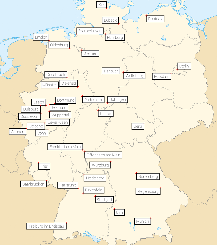
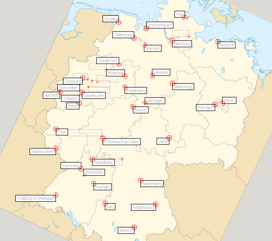
Figure 1: Instance with 43 labeled cities in Germany. Input labeling (left), rotated by $\sim 25^{\circ}$ (right).

Background picture is in public domain. Retrieved from Wikpedia [Link]

Been et al. [2, 3] defined a set of consistency desiderata for labeling zoomable dynamic maps, which include that (i) labels do not pop or flicker during monotone zooming, (ii) labels do not jump during the animation, and (iii) the labeling only depends on the current view and not its history. In our previous paper [8], we adapted the consistency model of Been et al. to rotating maps, showed NP-hardness and other properties of consistent labelings in this model, and provided efficient approximation algorithms.

Similar to the (NP-hard) label number maximization problem in static map labeling [6], the goal in dynamic map labeling is to maximize the number of visible or active labels integrated over one full rotation of $2\pi$. The value of this integral is denoted as the total activity and defines our objective function. Figure 1 shows an example seen from two different angles. Without any consistency restrictions, we can select the active labels for every rotation angle $\alpha\in[0,2\pi)$ independently of any other rotation angles. Clearly, this may produce an arbitrarily high number of flickering effects that occur whenever a label changes from active to inactive or vice versa. Depending on the actual consistency model, the number of flickering events per label is usually restricted to a very small number. Our goal in this paper is to evaluate several possible labeling strategies, where a labeling strategy combines both a consistency model and a labeling algorithm. First, we want to evaluate the loss in total activity caused by using a specific consistent labeling model rather than an unrestricted one. Second, we are interested in evaluating how close to the optimum total activity our proposed algorithms get for real-world instances in a given consistency model.

Related Work.

Most previous work on dynamic map labeling covers maps that allow panning and zooming, e.g., [2, 3, 10, 11, 12]; there is also some work on labeling dynamic points in a static map [5, 4]. As mentioned above, the dynamic map labeling problem for rotating maps has first been considered in our previous paper [8]. We introduced a consistency model, and proved NP-completeness even for unit-square labels. For unit-height labels we described an efficient 1/4-approximation algorithm as well as a PTAS. Yokosuka and Imai [14] considered the label size maximization problem for rotating maps, where the goal is to find the maximum font size for which all labels can be constantly active during rotation. Finally Gemsa et al. [7] studied a trajectory-based labeling model, in which a locally consistent labeling for a viewport moving along a given smooth trajectory needs be computed. Their model combines panning and rotation of the map view.

Our Contribution.

In this paper we take a practical point of view on the dynamic map labeling problem for rotating maps. In Section 2 we formally introduce the algorithmic problem and discuss our original rather strict consistency model [8], as well as two possible relaxations that are interesting in practice. Section 3 summarizes the known 1/4-approximation algorithm [8], introduces three greedy heuristics (one of which is a 1/8-approximation for unit square labels), and presents a formulation as an integer linear program (ILP), which provides us with optimal solutions against which to compare the algorithms. Our main contribution is the experimental evaluation in Section 4. We extracted several real-world labeling instances from OpenStreetMap data and make them available as a benchmark set. Based on these data, we evaluate both the trade-off between the consistency and the total activity, and the performance of the proposed labeling algorithms. The experimental results indicate that a high degree of labeling consistency can be obtained at a very small loss in activity. Moreover, our greedy algorithms achieve a high labeling quality and outperform the running times of the other methods by several orders of magnitude. We conclude with a suggestion of the most promising labeling strategies for typical use cases.

2 Preliminaries

In this section we describe a general labeling model for rotating maps with axis-aligned rectangular labels. This model extends our earlier model [8].

Let $M$ be an (abstract) map, consisting of a set $P=\{p_{1},\dots,p_{n}\}$ of points in the plane together with a set $L=\{\ell_{1},\dots,\ell_{n}\}$ of pairwise disjoint, closed, and axis-aligned rectangular labels in the plane. Each point $p_{i}$ must coincide with a corner of its corresponding label $\ell_{i}$; we denote that corner (and the point $p_{i}$) as the anchor of label $\ell_{i}$. Since each label has four possible positions with respect to $p_{i}$ this widely used model is known in the literature as the 4-position model (4P) [6].

As $M$ rotates, each label $\ell_{i}$ in $L$ must remain horizontally aligned and anchored at $p_{i}$. Thus, new label intersections form and existing ones disappear during the rotation of $M$. We take the following alternative perspective on the rotation of $M$. Rather than rotating the points, say clockwise, and keeping the labels horizontally aligned we may instead rotate each label counterclockwise around its anchor point and keep the set of points fixed. Both rotations are equivalent in the sense that they yield exactly the same intersections of labels and occlusions of points.

We consider all rotation angles modulo $2\pi$. For convenience we introduce the interval notation $[a,b]$ for any two angles $a,b\in[0,2\pi]$. If $a\leq b$, this corresponds to the standard meaning of an interval, otherwise, if $a>b$, we define $[a,b]:=[a,2\pi]\cup[0,b]$. For simplicity, we refer to any set of the form $[a,b]$ as an interval. We define the length of an interval $I=[a,b]$ as $|I|=b-a$ if $a\leq b$ and $|I|=2\pi-a+b$ if $a>b$.

A rotation of $L$ is defined by a rotation angle $\alpha\in[0,2\pi)$. We define $L(\alpha)$ as the set of all labels, each rotated by an angle of $\alpha$ around its anchor point. A rotation labeling of $M$ is a function $\phi\colon L\times[0,2\pi)\rightarrow\{0,1\}$ such that $\phi(\ell,\alpha)=1$ if label $\ell$ is visible or active in the rotation of $L$ by $\alpha$, and $\phi(\ell,\alpha)=0$ otherwise. We call a labeling $\phi$ valid if, for any rotation $\alpha$, the set of labels $L_{\phi}(\alpha)=\{\ell\in L(\alpha)\mid\phi(\ell,\alpha)=1\}$ consists of pairwise disjoint labels. If two labels $\ell$ and $\ell^{\prime}$ in $L(\alpha)$ intersect, we say that they have a (soft) conflict at $\alpha$, i.e., in a valid labeling at most one of them can be active at $\alpha$. We define the set $C(\ell,\ell^{\prime})=\{\alpha\in[0,2\pi)\mid\ell\text{ and }\ell^{\prime}\text{ are in conflict at }\alpha\}$ as the conflict set of $\ell$ and $\ell^{\prime}$. Further, we call a contiguous range in $C(\ell,\ell^{\prime})$ a conflict range. The begin and end of a maximal conflict range are called conflict events.

For a label $\ell$ we call each maximal interval $I\subseteq[0,2\pi)$ with $\phi(\ell,\alpha)=1$ for all $\alpha\in I$ an active range of label $\ell$ and define the set $A_{\phi}(\ell)$ as the set of all active ranges of $\ell$ in $\phi$. We call an active range where both boundaries are conflict events a regular active range. Our optimization goal is to find a valid labeling $\phi$ that shows a maximum number of labels integrated over one full rotation from $0$ to $2\pi$. The value of this integral is called the total activity $t(\phi)$ and can be computed as $t(\phi)=\sum_{\ell\in L}\sum_{I\in A_{\phi}(\ell)}|I|$. The problem of optimizing $t(\phi)$ is called total activity maximization problem (MaxTotal).

A valid labeling is not yet consistent in terms of the definition of Been et al. [2, 3]: while labels clearly do not jump and the labeling is independent of the rotation history, labels may still flicker multiple times during a full rotation from $0$ to $2\pi$, depending on how many active ranges they have in $\phi$. In the most restrictive consistency model, which avoids flickering entirely, each label is either active for the full rotation $[0,2\pi)$ or never at all. We denote this model as 0/1-model. In our previous paper [8] we defined a rotation labeling as consistent if each label has only a single active range, which we denote here as the 1R-model. This immediately generalizes to the $k$R-model that allows at most $k$ active ranges for each label. Analogously, the unrestricted model, i. e., the model without restrictions on the number of active ranges per label, is denoted as the $\infty$R-model.

We may apply another restriction to our consistency models, which is based on the occlusion of anchors. Among the conflicts in set $C(\ell,\ell^{\prime})$ we further distinguish hard conflicts, i.e., conflicts where label $\ell$ intersects the anchor point of label $\ell^{\prime}$. If a labeling $\phi$ sets $\ell$ active during a hard conflict with $\ell^{\prime}$, the anchor of $\ell^{\prime}$ is occluded. This may be undesirable in some situation in practice, e.g., if every point in $P$ carries useful information in the map, even if it is unlabeled. Thus we may optionally require that $\phi(\ell,\alpha)=0$ during any hard conflict of a label $\ell$ with another label $\ell^{\prime}$ at angle $\alpha$. Note that we can include other obstacles (e. g., important landmarks on a map) which must not be occluded by a label in form of hard conflicts. Note that a soft conflict is always a label-label conflict, while a hard conflict is always a label-point conflict (in our definition every label-point conflict induces also a label-label conflict). We showed earlier [8] that MaxTotal is NP-hard in the 1R-model avoiding hard conflicts and presented approximation algorithms.

3 Algorithmic Approaches

In this section we describe five algorithmic approaches for computing consistent active ranges that we evaluate in our experiments. Section 3.1 describes three simple greedy heuristics. Then, we sketch in Section 3.2 our 1/4-approximation algorithm which we described in more detail in [8]. It is based on the shifting technique by Hochbaum and Maass [9], where instances are decomposed into small independent cells that are then solved optimally. Finally, we give an ILP formulation in Section 3.3 that that we use primarily for evaluating the quality of the other solutions.

3.1 Greedy Heuristics

In this section we describe three new greedy algorithms to construct valid and consistent labelings with high total activity. These algorithms are conceptually simple and easy to implement, but in general we cannot give quality guarantees for the solutions computed by these algorithms.

All three greedy algorithms follow the same principle of iteratively assigning active ranges to all labels. The algorithm first initializes a set $L^{\prime}$ with all labels in $L$. Then it computes for each label $\ell$ its maximum active range $I_{\max}(\ell)$, which is the active range of maximum length $|I_{\max}(\ell)|$ such that (i) $\ell$ is not active while in conflict with another active label that was already considered by the algorithm, and (optionally) such that (ii) $\ell$ is not active while it has a hard conflict with another label. Initially the maximum active range of each label is either the full interval $[0,2\pi]$ or the largest range that avoids hard conflicts. Then the algorithm repeats the following steps. It selects and removes a label $\ell$ from $L^{\prime}$, assigns it the active range $I_{\max}(\ell)$, and updates those labels in $L^{\prime}$ whose maximum active range is affected by the assignment of $\ell$’s active range. If we consider the $k$R-model with $k>1$, we keep a counter for the number of selected active ranges and add another copy of $\ell$ with the next largest active range to $L^{\prime}$ if the counter value is less than $k$. The three algorithms differ only in the criterion that determines which label is selected from $L^{\prime}$ in each iteration.

The first algorithm we propose is called GreedyMax. In each step the algorithm selects the label with the largest maximum active range among all labels in $L^{\prime}$. Ties are broken arbitrarily. The second algorithm, GreedyLowCost, determines for the maximum active range of each label the cost of adding it to the solution. This means that for each label $\ell\in L^{\prime}$ with maximum active range $I_{\max}(\ell)$ the algorithm determines for all labels $\ell^{\prime}\in L^{\prime}$ that are in conflict with $\ell$ during $I_{\max}(\ell)$ by how much their maximum active range would shrink. The sum of this is the cost $c(\ell)$ of assigning the active range $I_{\max}(\ell)$ to $\ell$. Among all labels in $L^{\prime}$ GreedyLowCost chooses the one with lowest cost. Finally, the last algorithm, GreedyBestRatio is a combination of the two preceding ones. In each step the algorithm chooses the label $\ell$ whose ratio $|I_{\max}(\ell)|/c(\ell)$ is maximum among all labels in $L^{\prime}$. We conclude with a brief performance analysis of our algorithms.

Theorem 3.1

In the $k$R-model with constant $k$ the algorithm GreedyMax can be implemented to run in time $O(cn\cdot(c+\log n))$ and the algorithms GreedyLowCost and GreedyBestRatio can be implemented to run in time $O(cn\cdot(c^{2}+\log n))$, where $n$ is the number of labels and $c$ is the maximum number of conflicts per label in the input instance. The space consumption of all algorithms is $O(cn)$.

Proof

We begin by describing the time complexity for GreedyMax and sketch how to adapt the proof for GreedyBestRatio and GreedyLowCost.

For the initialization we need to compute the maximum active range for all labels which can be done in $O(cn)$ time. Note that this is only necessary in the hard-conflict model, since in the soft-conflict model the maximum active range is for all labels is the full rotation. To efficiently query for the label with longest maximum active range we maintain a maximum heap $H$ in which we store all labels from the set $L^{\prime}$ with the length of their maximum active range as key. Initially we need to add all labels from $L$ into $H$, which requires $O(n\log n)$ time.

In each step of the algorithm it first selects the label $\ell$ with maximum active range still left in $L^{\prime}$. Then, it needs to update the maximum active range of those labels in $L^{\prime}$ that have a conflict with $\ell$. Since we maintain all labels contained in $L^{\prime}$ in the heap $H$, we can find and remove the label with maximum active range in $L^{\prime}$ in $O(\log n)$ time. To determine the new maximum active ranges for those labels in $L^{\prime}$ that are in conflict with $\ell$, we conduct a simple linear sweep over $[0,2\pi)$. Note that there are at most $O(c)$ conflict events and hence a single sweep requires $O(c)$ time. Finally, we need to update the value of the maximum active ranges in the global heap. This requires $O(c\log n)$ time. Thus, a single step in the algorithm requires $O(c^{2}+c\log n)$ time. Since there are $n$ steps, the claimed running time follows.

For GreedyLowCost and GreedyBestRatio we use the same approach, but we store the labels with their cost and gain-cost ratio as key, respectively. The main difference compared to GreedyMax is the necessity to compute the cost of selecting a maximum active range, which can be done straightforwardly in $O(c^{2})$ time per label. After selecting a label and assigning it its maximum active range, the maximum active ranges of at most $O(c)$ labels still left in $L^{\prime}$ may change. For these labels, the algorithm needs to recompute the cost of selecting their maximum active ranges and update these values in the maximum heap. In total a single step for GreedyLowCost or GreedyBestRatio requires $O(c^{3}+c\log n)$ time. The claimed time complexity follows. The required space is dominated by the storage required to store for each label its relevant conflict events. This takes $O(cn)$ space.

By using a more efficient encoding of the maximal disjoint intervals that can be assigned to label $\ell_{i}$ in a heap, the running time of GreedyMax can be further improved to $O(cn\log n)$.

Theorem 3.2

GreedyMax can be implemented with time complexity $O(cn\log n)$ and space requirement in $O(cn)$.

Proof

Similar to the proof of Theorem 3.1, we maintain a global heap that contains the maximum possible active range for each label. In the following we describe the modified representation of the possible active ranges for the individual labels.

We maintain for each label $\ell_{i}\in L$ a maximum heap $H_{i}$ that maintains all maximal disjoint intervals the label $\ell_{i}$ can be assigned as active range. Further, each label also maintains a balanced binary tree $T_{i}$ on the same set of intervals, i. e., we store the left and right endpoints of the intervals in $T_{i}$. Should one of the intervals span over $2\pi$, we split it into two intervals at $2\pi$. Since there are $O(c)$ conflict events per label, both $T_{i}$ and $H_{i}$ can contain at most $O(c)$ elements.

For the initialization we first need to compute all possible maximal active ranges for each label which can be done in $O(cn)$ time. Initializing the global heap can be done as before in $O(n\log n)$ time, and since each label specific heap $H_{i}$ and binary tree $T_{i}$ can contain at most $O(c)$ elements, their initialization requires $O(cn\log c)$ time in total.

Now, when the algorithm has chosen a label $\ell$ with maximum active range $A(\ell)$ with left and right endpoints $a$ and $b$, respectively, it needs to update the maximum active range of each label $\ell_{i}$ that is in conflict with $\ell$. So, for each label $\ell_{i}$ in conflict with $\ell$, we query $\ell_{i}$’s binary search tree $T_{i}$ with $a$ and $b$. This allows us to obtain all $k$ maximal intervals of $\ell_{i}$ that partly overlap with, or are completely contained in $A(\ell)$. The intervals completely contained in $A(\ell)$ need to be removed from $T_{i}$ and $H_{i}$, while the intervals (at most two) that are only partly contained in $A(\ell)$ are shrunk or split.

The query on the binary search tree requires $O(k+\log c)$ time, where $k$ is the number of reported intervals. Updating both $T_{i}$ and $H_{i}$ requires then $O(\log c)$ time for the intervals that get shrunk (or split). Deleting the elements is more costly, but since in both the binary tree as well as the heap there can be at most $O(c)$ elements, and we insert and remove each element at most once, we can conclude that inserting and deleting requires per binary tree and heap each in total at most $O(c\log c)$ time. Since there are $O(n)$ heaps and trees, this requires in total $O(cn\log c)$ time.

We now summarize these results. The initialization can be done in $O(cn\log n)$ time. In each step we require $O(\log n)$ time to determine and remove the label $\ell$ with maximum active range from the global heap. Then, we shrink or split the intervals of labels that are in conflict with $\ell$ in $O(c\log c)$ time. We need to update the global heap since the maximum active range of the $O(c)$ labels that are in conflict with $\ell$ might have changed. This update requires $O(c\log n)$ time. Finally, we need to repeat this step $O(n)$ times, yielding $O(cn(\log c+\log n))=O(cn\log n)$ time. As stated above, the insertion and deletion into the label’s own binary trees and maximum heaps requires in total $O(cn\log n)$ time, yielding a total time complexity of $O(cn\log n)$. The space consumption is dominated by the $O(n)$ trees, each of size $O(c)$. Thus the algorithm requires $O(cn)$ space.

Approximation for Unit Square Labels.

Although it was stated at the beginning of the Section 3.1 that, in general, we cannot prove any quality criteria for the presented algorithms, for the special case that labels are unit squares, we can show that GreedyMax is an approximation algorithm with approximation ratio $1/8$. This is due to a result by Gemsa et al. [7, Lemma 1 and Lemma 2] in which the authors consider a similar problem. The results of both Lemmas imply the following.

Lemma 1 ([7], Lemmas 1 and 2)

Let $L$ be a set of unit square labels and let $\ell\in L$. For any rotation angle $\alpha\in[0,2\pi)$ there are at most eight pairwise disjoint unit square labels in $L(\alpha)$ that overlap with $\ell$.

Since, in each step of the GreedyMax algorithm, we select the label $\ell$ with maximum active range, we can conclude by Lemma 1 that the cost of choosing $\ell$ is at most eight times its maximum active range. We summarize this in the following.

Corollary 1

GreedyMax is a 1/8-approximation algorithm for MaxTotal in the case that all labels are unit squares.

3.2 1/4-Approximation Algorithm

Our previous 1/4-approximation [8] is based on the line stabbing or shifting technique by Hochbaum and Maass [9], which has been applied before to static labeling problems for (non-rotating) unit-height labels, e. g., [1, 5, 13]. We sketch the idea of the algorithm for unit squares, but note that it applies in a similar way to rectangular labels with bounded aspect ratio and that it can be generalized to a PTAS [8]. The first step of the algorithm is to subdivide the plane into square grid cells with side length $2\sqrt{2}$. Each cell is addressed by a row and column index. We obtain a partition of the initial instance into four different subsets by deleting the points in every other row and every other column. In each subset the cells now have a distance to each other that is at least $2\sqrt{2}$ and thus, labels that are in different cells cannot intersect each other; see Figure 2. Note that for hard conflicts we need to consider the area within distance $\sqrt{2}$ of each cell. If we solve all four subsets optimally, at least one of the solutions is a 1/4-approximation for the entire instance due to the pigeon-hole principle.

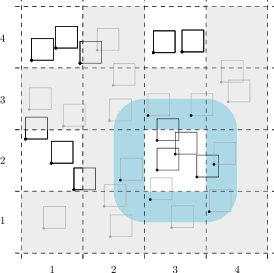
Figure 2: Plane divided into grid cells. Cells of one subinstance are marked white. The blue area has distance at most $\sqrt{2}$ to the cell (3, 2).

To find the optimal solution for a single grid cell we observed that there can only be a constant number of labels in each grid cell [8]. Further, we observed that this implies that also the number of conflict events in each grid cell is constant which int combination with [8, Lemma 4] means that the optimal solution can be obtained by a simple brute force approach in $O(1)$ time per cell, which results in an overall running time of $O(n\log n)$.

3.3 Integer Linear Program

In this section we present an ILP-based approach to find optimal solutions for MaxTotal. This is justified since MaxTotal is NP-hard and we cannot hope for an efficient algorithm unless $P=NP$. We note that the same ILP formulation can also be used in the 1/4-approximation algorithm to compute an optimal solution within each grid cell. The ILP formulation given is similar to that of Gemsa et al. [7].

The key idea of the ILP presented here is to determine regular active ranges induced by the ordered set of all conflict events. Our model contains for each label $\ell$ and each interval $I$ a binary decision variable, which indicates whether or not $\ell$ is active during $I$. We add constraints to ensure that (i) no two conflicting labels are active at the same time within their conflict range and (ii) at most $k$ disjoint contiguous active ranges can be selected for each label as required in the $k$R-model.

Model.

For simplicity we assume in this section that the length of each conflict range is strictly larger than 0. This assumption is not essential for our ILP formulation, but makes the description easier.

Let $E$ be the ordered set of conflict events that also contains 0 and $2\pi$, and let $E[j]$ be the interval between the $j$-th and the $(j+1)$-th element in $E$. We call such an interval $E[j]$ an atomic interval and always consider its index $j$ modulo $|E|-1$. For each label $\ell_{i}\in L$ and for each atomic interval $E[j]$ we introduce two binary variables $x_{i}^{j}$ and $b_{i}^{j}$ to our model. We refer to the variables of the form $x_{i}^{j}$ as activity variables. The intended meaning of $x_{i}^{j}$ is that its value is 1 if and only if the label $\ell_{i}$ is active during the $j$-th atomic interval; otherwise $x_{i}^{j}$ has value 0. We use the binary variables $b_{i}^{j}$ to indicate the start of a new active range and to restrict their total number to $k$. This is achieved by adding the following constraints to our model.

$$x_{i}^{j}-b_{i}^{j} \leq x_{i}^{j-1} \forall\ell_{i}\in L\quad\forall j\in\{0,\dots,|E|-2\}$$ (1)

$$\sum_{0\leq j\leq|E|-2}b_{i}^{j} \leq k \forall\ell_{i}\in L$$ (2)

The effect of constraint (1) is that it is only possible to start a new active range for label $\ell_{i}$ with atomic interval $E[j]$ (i.e., $x_{i}^{j-1}=0$ and $x_{i}^{j}=1$) if we account for that range by setting $b_{i}^{j}=1$. Due to constraint (2) this can happen at most $k$ times per label. We can also allow arbitrarily many active ranges per label as in the $\infty$R-model by completely omitting the variables $b_{i}^{j}$ and the above constraints.

It remains to guarantee that no two labels can be active when they are in conflict. This can be done straightforwardly since we can compute for which atomic intervals two labels are in conflict and we ensure that not both activity variables can be set to 1. More specifically, for every pair of labels $\ell_{i},\ell_{k}$ and for every atomic interval $j$ during which they are in conflict, we add the constraint

$$x_{i}^{j}+x_{k}^{j}\leq 1.$$ (3)

Optionally, incorporating hard conflicts can also be done easily as a hard conflict simply excludes certain atomic intervals from being part of an active range. We determine for each label all such atomic intervals in a preprocessing step and set the corresponding activity variables to 0.

Among all feasible solutions that satisfy the above constraints, we maximize the following objective function: $\sum_{\ell_{i}\in L}\sum_{0\leq j\leq|E|-2}x_{i}^{j}\cdot|E[j]|$, which is equivalent to the total activity $t(\phi)$ of the induced labeling $\phi$.

This ILP considers only regular active ranges, since label activities change states only at conflict events. However, by [8, Lemma 4], there always exists an optimal solution that is regular, and hence we are guaranteed to find a globally optimal solution.

Minimizing the Number of Active Ranges in the ILP.

In Section 2 we explained that, in order to reduce flickering, we require that each label has at most one active range. However, we might be able to reduce flickering even more by finding among all optimal solutions the one that has the fewest active ranges. We can modify our ILP to accommodate for this by modifying the objective function slightly. Let $s>0$ denote the length of a shortest atomic interval (recall that all atomic intervals are assumed to have positive length). Thus, whenever a label is active during an atomic interval, the total activity increases by at least $s$. To minimize the number of active ranges, we substract $s/2$ from the objective function for each active range. In this way, a solution with larger total activity is always preferred over a solution with less total activity, while among two solutions with the same total activity the one with fewer active ranges has the greater objective value. Hence, to minimize the number of active ranges while maintaining optimality, we modify the objective function to $\sum_{\ell_{i}\in L}\sum_{0\leq j\leq|E|-2}\left(x_{i}^{j}\cdot|E[j]|-b_{i}^{j}\cdot s/2\right)$. To ensure that if label $\ell_{i}$ is active at any time, then at least one of the variables $b_{i}^{j}$ is $1$, we also add the following constraints.

$$(|E|-1)\cdot\sum_{j=0}^{|E|-2}b_{i}^{j}\geq\sum_{j=0}^{|E|-2}x_{i}^{j} \forall\ell_{i}\in L$$ (4)

Without this constraint, it would be possible to have a label $\ell_{i}$ active for the whole range $[0,2\pi)$ but with $b_{i}^{j}=0$ for all $j\in\{0,\dots,|E|-2\}$. We note that it follows from the proof of Lemma 4 in [8] that also for the modified problem there always exists an optimal solution that is regular. Hence an optimal solution to the above ILP is indeed a global optimum.

We have now given a complete description of our ILP model, and now turn towards the analysis of the number of variables and constraints necessary for our model. Let $e$ be the number of conflict events and $c$ be the maximum number of conflict events per label in a MaxTotal instance, respectively. In the worst case the number of constraints that ensure that the solution is conflict-free (i. e., constraint (3)) is $O(c\cdot e)$ per label, whereas we require only $O(e)$ constraints of the other types of constraints per label. We conclude the results of this section in the following theorem.

Theorem 3.3

The ILP (1)–(3) solves MaxTotal and has at most $O(e\cdot n)$ variables and $O(c\cdot e\cdot n)$ constraints, where $n$ is the number of labels, $e$ the number of conflict events, and $c$ the maximum number of conflicts per label.

4 Experimental Evaluation

In this section we present the experimental evaluation of different labeling strategies based on the consistency models and algorithms introduced in Sections 2 and 3. We implemented our algorithms in C++ and compiled with GCC 4.7.1 using optimization level -O3. As ILP solver we used Gurobi 5.6. The running time experiments were performed on a single core of an AMD Opteron 2218 processor running Linux 2.6.34.10. The machine is clocked at $2.6\,\mathrm{GHz}$, has $16\,\mathrm{GiB}$ of RAM and $2\times 1\,\mathrm{MiB}$ of L2 cache. Before we discuss our results we introduce the benchmark instances. The reported running times in the following are always measured as wall-clock time (as opposed to pure CPU time).

4.1 Benchmark Instances

Since our labeling problem is immediately motivated by dynamic mapping applications, we focus on gathering real-world data for the evaluation. As data source we used the publicly available data provided by the OpenStreetMap project. We extracted the latitudes, longitudes and names of all cities with a population of at least $50\,000$ for six countries (France, Germany, Italy, Japan, United Kingdom, and the United States of America) and created maps at three different scales.

To obtain a valid labeling instance several additional steps are necessary. First, the width and height of each label need to be chosen. Second, we need to map latitude and longitude to the two-dimensional plane. Third, recall that the input is a statically labeled map, and hence we need to compute such a static input labeling. For the first issue we used the same font that is used in Google Maps, i. e., Roboto Thin. The dimensions of each label were obtained by rendering the label’s corresponding city name in Roboto Thin with font size 13, computing its bounding box, and adding a small additional buffer. For obtaining two-dimensional coordinates from the latitude and longitude of each point, we use the popular Mercator projection. For the map scales we again wanted to be close to Google Maps. Hence, we used the Mercator projection (where we approximate the ellipsoid with a sphere of radius $r=6371$km) for three different scales (65 pixel $\widehat{=}$ 20km, 50km, 100km) for each country. For simplicity we refer to the scale of 65 pixel $\widehat{=}$ 20km only by 20km (and likewise for the remaining scales). The last remaining step was to compute a valid input labeling. For this we used the 4P fixed-position model [6] and solved a simple ILP model to obtain a weighted maximum independent set in the label conflict graph, in which any two conflicting label positions are linked by an edge and weights are proportional to the population. Table 1 shows the characteristics of our benchmark data.

We also obtained much larger instances than the country instances described in Table 1. We chose Berlin, New York, London, and Paris and extracted the names, as well as longitude and latitude, of all restaurants in each of these cities from OpenStreetMap. To obtain valid input data we conducted the same steps as described for the country instances with Roboto Thin but with font size 8 and the three scales 65pixel $\widehat{=}$ 20m, 50m, 100m. We report the number of labels for these instances in Table 2.

Both sets of benchmark data can be downloaded from our website.

Table 1: Number of labels in each country instance, the number of labels in the largest connected component (lcc) and the number of connected components (cc) in the conflict graph.

	countries
	FR	DE	GB	IT	JP	US
scales	#labels (#labels in lcc / #cc)
20km	86 (12/51)	52 (20/26)	99 (73/19)	131 (28/48)	99 (12/34)	403 (26/203)
50km	80 (39/9)	43 (39/4)	68 (66/2)	111 (87/5)	80 (69/7)	359 (88/89)
100km	69 (69/1)	33 (33/1)	37 (37/1)	68 (68/1)	49 (44/3)	288 (213/16)

Table 2: Number of labels in each city instance, the number of labels in the largest connected component (lcc) and the number of connected components (cc) in the conflict graph.

	cities
	Berlin	New York	London	Paris
scales	#labels (#labels in lcc / #cc)
20m	2744 (13/2205)	629 (9/445)	1661 (40/1044)	2367 (39/1560)
50m	2739 (77/1329)	621 (50/279)	1620 (175/569)	2325 (244/703)
100m	2628 (416/634)	602 (88/143)	1457 (371/289)	2141 (952/230)

4.2 Evaluation of the Consistency Models

In this section we evaluate the different consistency models introduced in Section 2. The models differ by the admissible number of active ranges per label and the handling of hard conflicts. We begin by analyzing the effect of limiting the number of active ranges and consider the five models 0/1, 1R, 2R, 3R, and $\infty$R, all taking hard conflicts into account. As discussed in Section 2, the 0/1-model is flicker-free but expected to have a low total activity, especially in dense instances. On the other hand, the $\infty$R-model achieves the maximum possible total activity in any valid labeling, but is likely to produce a large number of flickering effects. Still, it serves as an upper bound on the total activities of the other models. The two most important quality criteria in our evaluation are (i) the total activity of the solution, and (ii) the average length of the active ranges. Unfortunately, it proved too time consuming for our ILP to solve the city instances in a reasonable time frame. Thus, we chose to restrict ourselves in this analysis to the country instances described in Table 1.

Table 3: Average total activity of the optimal solutions for the country instances with respect to the maximum possible objective value with standard deviation in brackets. Instances grouped by scale. Additionally we report the average interval length normalized to one full rotation, and for the $\infty$R-model the average number of intervals per label.

model	0/1		1R			2R			3R			$\infty$R
scale	total act.		total act.	$\sim$len		total act.	$\sim$len		total act.	$\sim$len		$\sim$len	$\sim$intervals
20km	54.04% (12.62)		94.56% (2.85)	0.76		99.36% (0.64)	0.56		99.92% (0.10)	0.47		0.08	19.13
50km	22.42% (11.74)		87.79% (4.44)	0.58		97.69% (1.95)	0.35		99.54% (0.69)	0.26		0.01	79.23
100km	6.19% (5.06)		81.01% (2.15)	0.44		95.83% (1.56)	0.27		99.24% (0.36)	0.19		0.01	128.40

(a) Hard-conflict model.

model	0/1		1R			2R			3R			$\infty$R
scale	total act.		total act.	$\sim$len		total act.	$\sim$len		total act.	$\sim$len		$\sim$len	$\sim$intervals
20km	69.18% (8.14)		98.17% (1.20)	0.83		99.79% (0.19)	0.64		99.98% (0.02)	0.59		0.54	1.80
50km	49.47% (5.54)		94.80% (1.96)	0.69		99.27% (0.69)	0.44		99.86% (0.22)	0.37		0.27	5.09
100km	42.41% (3.12)		91.67% (1.59)	0.58		98.57% (0.40)	0.34		99.76% (0.07)	0.24		0.07	9.55

(b) Soft-conflict model.

In Table 3(a) we report the total activity of the optimal solution for the tested models relative to the solution in the $\infty$R-model. The results of the instances are aggregated by scale. We observe that the total activity of the 0/1-model drops to less than 55% compared to the optimal solution in the $\infty$R-model even for the least dense instance at scale 20km and to only 6% for a scale of 100km. Hence this model is of very little interest in practice.

We see a strong increase in the average total activity values already for the 1R-model compared to the optimal solution in the 0/1-model. For the large-scale instance 20km 1R reaches almost 95% of the $\infty$R-model, which has more than 19 times the number of flickering effects and active ranges of average length shorter by a factor of $1/9$. For map scales of 50km and 100km, the total activities drop to 88% and 81%, respectively, but at the same time the number of flickering effects and the average active range lengths in the $\infty$R model are extremely poor. Thus the 1R-model achieves generally a very good labeling quality by using only one active range per label.

Finally, we take a look at the middle ground between the 1R- and the $\infty$R-models. It turns out that total activity of the 2R-model is off from the $\infty$R-model by less than 1% at scale 20km and less than 5% at scale 100km, but this increase in activity over the 1R model comes at the cost of producing twice as many flickering effects and decreasing the average active range length by 30–40%. If we allow three active ranges per label, the total activity increases to more than 99% of the upper bound in the $\infty$R-model at all three scales, while having significantly fewer flickering effects and longer average active ranges. The activity gain by considering the $k$R-model for $k>3$ is negligible and the disadvantage of increasing the number of flickering effects dominates.

When we conduct the same analysis for the 0/1, 1R, 2R, and $\infty$R model in the soft-conflict model, similar trends can be observed. We report in Table 3(b), analogous to Table 3(a), the total activity of the optimal solution for the tested models relative to the solution in the $\infty$R-model. We observe that the trend in both tables is similar. However, the 0/1-model performs in general significantly better than in the hard-conflict model, but the results are still not suitable from a practical point of view. Already the 1R model produces results which are close to the maximum possible solution in the $\infty$R-model, while the difference in the optimal solutions in the 2R and 3R-model to the $\infty$R-model are negligible.

We conclude that the 1R-model achieves the best compromise between total activity value and low flickering, at least for maps at larger scales with lower feature density. For dense maps the 2R- or even the 3R-models yield near-optimal activity values while still keeping the flickering relatively low. Going beyond three active ranges per label only creates more flickering but does not provide noticeable additional value.

It remains to investigate the impact of hard conflicts. For this we apply the 1R-model and compare the variant where all conflicts are treated equally (soft-conflict model) with the variant where hard conflicts are disallowed (hard-conflict model). For this we consider for each map scale the average relative increase in activity value of the soft-conflict model over the stricter hard-conflict model. For 20km instances the increase is on average $8.51\%$ (standard deviation 2.91), for the intermediate scale 50km it is on average $19.25\%$ (standard deviation 7.86), and for the small-scale map 100km the increase reaches on average $31.9\%$ (standard deviation 4.72). These results indicate that, unsurprisingly, the soft-conflict model improves the total activity at all scales, and in particular for dense configurations of point features, where labels usually have several hard conflicts with nearby features. As discussed before, this improvement comes at the cost of temporarily occluding unlabeled but possibly important points. It is an interesting open usability question to determine user preferences for the two models and the actual effect of temporary point occlusions on the readability of dynamic maps, but such a user study is out of scope of this evaluation and left as an interesting direction for future work.

4.3 Evaluation of the Algorithms

In this section we evaluate the quality (total activity) and running time of the 1/4-approximation algorithm and the three greedy heuristics GreedyMax, GreedyLowCost, and GreedyBestRatio (Section 3.1), which we abbreviate as QAPX, GM, GLC, and GBR, respectively. Additionally, we include the ILP (Section 3.3) as the only exact method in the evaluation. The ILP is also applied to optimally solve the independent subinstances in the grid cells created by QAPX. In our implementation we heuristically improve the running time of the ILP by partitioning the conflict graph of the labels into its connected components and solving each connected component individually; see Table 1 for the number of labels in the largest connected component and the number of connected components in the conflict graph of each instance. For the ILP we set a time limit of 1 hour and restrict the ILP solver to a single thread. The same restrictions are applied to the ILP when solving the small subinstances in algorithm QAPX. By the design of the algorithm, a solution obtained by QAPX will consist of many labels that have no active range, although they could be assigned one (all labels that are discarded to obtain independent cells have active range set to length 0). To overcome this drawback, we propose a combination of QAPX with the greedy algorithms. More specifically, we apply one of our greedy algorithms to each of the four solutions computed by the 1/4-approximation and determine among the four resulting solutions the best one. In the following we refer to the combination of the 1/4-approximation with a greedy algorithm by adding a Q in front of the greedy algorithm’s name (e. g., QGLC). We report the results of the algorithms for both the 1R soft-conflict and the 1R hard-conflict model, which turned out as a reasonable compromise between low flickering and high total activity in Section 4.2.

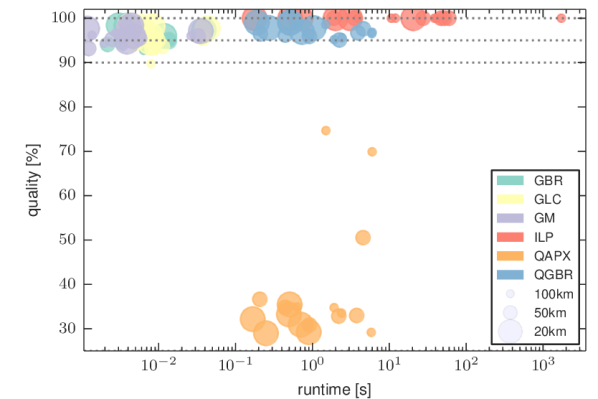
(a) Hard-conflict model.

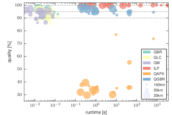
(b) Soft-conflict model.

Figure 3: Plot of the runtime (log scale) and quality results of the algorithm evaluation for the city instances in the 1R hard-conflict and soft-conflict model.

We give a general overview of the performance of all evaluated algorithms as a scatter plot in Figure 3. In this scatter plot each disk represents the result of an algorithm (indicated by color) applied to a single country instance. The size of the circle indicates the scale of the instance (the smaller the circle, the smaller the scale). We omitted the algorithms QGM and QGLC in this plot to increase readability, because the difference in running time and quality of the solutions between the three algorithms QGM, QGLC, and QGBR is negligible and creates extra overplotting.

Soft-conflict model.

In Figure 3(b) we present an overview of the performance of the evaluated algorithms in the 1R soft-conflict model. We observe that the performance of the greedy algorithms is very good with respect to running time as well as quality of the solutions. As expected, the total activity of QAPX is always better than $25\%$, but generally much worse than for the remaining algorithms. It never gets close to the solutions produced by the greedy algorithms while being considerably slower. However, combining QAPX with a greedy algorithm achieves better solutions than greedy algorithms and QAPX alone, while the increase in running time over QAPX is negligible. Finally, we observe that the ILP solves the tested instances in a reasonable time frame. To obtain the optimal solution, the ILP required on average 758s, with a median of only 30.65s. However, we concede that larger instances may require significantly more time to solve, and there may be a threshold for which the use of the ILP is infeasible.

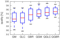
(a) Quality of the solutions as a percentage of the (optimal) ILP solution.

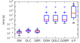
(b) Runtime (log scale) of the algorithms.

Figure 4: Performance of the greedy algorithms and QAPX with greedy postprocessing in the 1R soft-conflict model.

We now turn to a more detailed analysis of the two most promising approaches (i) using the greedy algorithms, and (ii) combining QAPX with the greedy algorithms in the soft-conflict model. For a detailed depiction of the performance of the algorithms with respect to the quality of the solution see the diagrams in Figure 4. We observe that among the three greedy algorithms GBR performs best with respect to quality with an average of $93.7\%$, but the difference to the other greedy algorithms is small. Even the greedy algorithm GM with the lowest total activity produces solution with an average of 91.8% of the optimal solution. Each of the combinations of QAPX with subsequent execution of a greedy algorithm outperforms each of the greedy algorithms alone in terms of quality. However, since the solutions produced by the greedy algorithms are already very close to the optimal solution, we observe only a slight increase in total activity for QGM, QGLC, and QGBR over the greedy algorithms. The difference between both approaches becomes much more visible when considering the running time. While the average running time for the three greedy algorithms is between 2.5ms and 3.9ms, the average running time for the 1/4-approximation algorithms is roughly 46s. However, we note that this large difference is mostly caused by one instance, which required over 664s to find the solution. The median running time for the enriched 1/4-approximation algorithms is about 1.08s.

Hard-conflict model.

In Figure 3(a) we present a general overview of the performance of the evaluated algorithms in the 1R hard-conflict model. Again, we omit QGLC, and QGM in the figure to increase readability.

The performance characteristics of the algorithms in this model resembles those in the soft-conflict model closely. The greedy algorithms perform, again, very well with respect to both running time and total activity. The combination of 1/4-approximation and greedy heuristics outperforms the greedy heuristics in total activity again, but is also significantly slower. Only the performance of ILP differs much from its performance in the soft-conflict model. To obtain an optimal solution the ILP required on average 114s, with a median of only 11.32s (compared to an average of 758s with a median of 30s). This is most likely caused by a decreased size in solution space, since in the hard-conflict model, some of the ILP’s activity variables are already initially required to be set to 0.

We again discuss the two most promising approaches in more detailed, but this time for the hard-conflict model, see Figure 5. Among the three greedy heuristics the simplest algorithm (i. e., GM) performs best with respect to quality with an average of $96\%$, but as a whole the greedy algorithms perform similarly well. Even the worst greedy algorithm GLC produces solutions of high quality (average is 95%). Each of the combinations of the 1/4-approximation with subsequent execution of a greedy algorithm outperforms each of the greedy algorithms alone. However, since the solutions produced by the greedy algorithms are so close to the optimal solution (even closer than in the soft conflict model), we observe only a slight increase in the quality of the solution for QGM, QGLC, and QGBR. Again, the difference is much more noticeable when considering the running time. While the average running time for the three greedy algorithms is between 7ms and 13ms, the average running time for the 1/4-approximation is roughly 1.8s with a median of 0.96s. We note an increase in the running time of the greedy algorithms compared to the soft-conflict model. However, all three algorithms are still very fast and suitable for real-time applications. For the combination of the 1/4-approximation and the greedy algorithms, with the exception of one instance, the running time of the 1/4-approximation in the 1R hard-conflict model is very similar to the running time in the 1R soft-conflict model. This might be surprising since the running time of the 1/4-approximation is dominated by obtaining optimal solutions for all of the subinstances by the ILP, which performs better in the hard-conflict model. We conjecture that this is because the subinstances required for the 1/4-approximation are very small and thus the performance increase is not that noticeable.

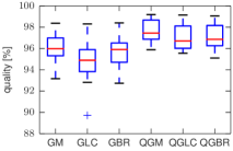
(a) Quality of the solutions as a percentage of the (optimal) ILP solution.

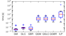
(b) Runtime (log scale) of the algorithms.

Figure 5: Performance of the greedy algorithms and QAPX with greedy postprocessing in the 1R hard-conflict model.

Additional Instances.

Recall that we presented besides the set of country instances also the city instances, which we did not use for evaluation so far. Note that these instances (described in Table 2) are much larger than the country instances. Unfortunately, for almost all of these instances we were not able to obtain optimal solutions in the 1R-model with the ILP in a reasonable time frame. We therefore cannot compare the quality of the obtained solutions by the greedy algorithms, and by the combination of 1/4-approximation and greedy algorithms with the optimal solution. Instead, we chose to compare the results of the algorithms with the optimal solution in the $\infty$R-model, which serves as an upper bound on the optimal solution in the 1R-model; see Table 4.

Table 4: Evaluation of the three greedy algorithms, and the combination of 1/4-approximation with the greedy algorithms for the restaurant instances; see Table 2. We compare the total activity of the solutions with the optimal solution in the $\infty$R-model. Table 4(a) reports the results for the 1R soft-conflict model, and Table 4(b) reports the results for the 1R hard-conflict.

(a) 1R soft-conflict model.

	algorithms
	GM		GLC		GBR		QGM		QGLC		QGBR
scales	time	total act.	time	total act.	time	total act.	time	total act.	time	total act.	time	total act.
20m	0.03s	97.69%	0.03s	98.01%	0.03s	98.58%	1.30s	98.21%	1.30s	98.44%	1.31s	98.70%
50m	0.03s	93.88%	0.04s	94.45%	0.04s	95.52%	238.50s	95.04%	238.52s	95.52%	238.52s	95.82%
100m	0.03s	89.36%	0.05s	89.90%	0.06s	91.39%	1124.23s	91.18%	1124.28s	91.33%	1124.29s	92.02%

(b) 1R hard-conflict model.

	algorithms
	GM		GLC		GBR		QGM		QGLC		QGBR
scales	time	total act.	time	total act.	time	total act.	time	total act.	time	total act.	time	total act.
20m	0.72s	97.23%	0.80s	97.20%	0.80s	97.39%	4.29s	97.53%	4.30s	97.55%	4.29s	97.58%
50m	0.79s	92.45%	0.86s	92.21%	0.87s	92.53%	16.91s	92.99%	16.94s	92.93%	16.94s	92.92%
100m	0.78s	87.05%	0.85s	86.09%	0.86s	86.61%	54.50s	87.56%	54.56s	86.96%	54.58s	87.17%

We observe that the results for all algorithms in both models are very close to the maximal achievable total activity in the $\infty$R model. Even in the most dense instance in the 1R hard-conflict model, the worst greedy algorithm achieves still on average about 86% of the maximal achievable total activity with a running time of about 0.8s. The quality of the greedy algorithms is slightly better in the 1R soft-conflict model and the running time is much smaller (around 30–40ms). The combination of 1/4-approximation and greedy heuristic does perform slightly better, but the difference is minuscule. However, the running time differs drastically. While in the country instances before, the average running time was less than 1s in both the 1R hard-conflict and the 1R soft-conflict model, the running time for the combination of 1/4-approximation and greedy heuristic is much slower. For the most dense instances the running time is on average one minute in the hard-conflict model and for the soft-conflict model about 20 minutes. However, at this point we need to mention that the running times for the instances vary quite significantly and the only conclusion we can draw safely from the detailed data is that this approach is much slower (even for the easiest instance the approach required for the soft-conflict model about 1 minute to compute the solution), but drawing conclusions beyond this is impossible.

The results indicate that the greedy algorithms in the 1R soft-conflict model produce solutions that are very close to the maximum possible total activity while the algorithms require only few milliseconds in running time. This strengthens our conclusion that the 1R model in combination with any of the three greedy algorithms is the best strategy for labeling rotating maps. Whether to use the soft-conflict model or the hard-conflict model is a design choice that should depend on the requirements of the actual application.

In order to give a final recommendation for an algorithm, it is necessary to make a choice on the time-quality trade-off that is acceptable in a particular situation. If running time is not the primary concern, e.g., for offline applications with high computing power available, we can recommend the ILP, which ran reasonably fast in our experiments, at least for the smaller country instances. On the other hand, if computing power is limited, instances are large, or real-time labeling is necessary, e.g., on a mobile device, all three greedy heuristics can be recommended as the methods of choice; a slight advantage of GBR was observed in our experiments. All three algorithms run very fast (a few milliseconds) and empirically produce high activities of more than $90\%$ of the optimum solution. If one wants to invest some extra running time, the combination of QAPX with a greedy algorithm may be of interest as it produces slightly better solutions than the stand-alone greedy algorithms and is much faster than the ILP.

5 Conclusion

In this work, we evaluated different strategies for labeling dynamic maps that allow continuous rotation, where a labeling strategy consists of a consistency model and a labeling algorithm. In the first part of the evaluation, we considered the quality of optimal solutions in different consistency models. It turned out that the restriction to one or two active ranges per label (1R- and 2R-models) yields the best compromise in terms of low flickering and high total activity value of more than 95% of the upper bound obtained from the unrestricted model ($\infty$R). Additionally, treating all pairwise label conflicts as soft conflicts increased the total activity values between 8% and 32% at the cost of occasional occlusion of unlabeled point features.

In the second part of the evaluation, we investigated the performance of three new greedy heuristics and our previous 1/4-approximation algorithm [8] in terms of labeling quality and running time. It turned out that the greedy heuristics performed very well in both total activity (well above 90%) and running time (a few ms). The unmodified 1/4-approximation performs much worse, but the combination of 1/4-approximation and greedy heuristics yields slightly higher total activity than the greedy heuristics alone; the running time, however, can grow to several seconds. In conclusion, we believe that the 1R model in combination with any of the three greedy algorithms is, in most cases, the best labeling strategy for labeling dynamic rotating maps. Whether the soft-conflict or the hard-conflict model is more appropriate depends on requirements of the application.

Acknowledgments

We thank an anonymous reviewer of the SEA 2014 version of this paper for the helpful and detailed comments. This work was partially supported by a Google Research Award.

References

- [1] P. K. Agarwal, M. van Kreveld, and S. Suri. Label Placement by Maximum Independent Set in Rectangles. Comput. Geom. Theory Appl., 11:209–218, 1998.
- [2] K. Been, E. Daiches, and C. Yap. Dynamic map labeling. IEEE Trans. Visualization and Computer Graphics, 12(5):773–780, 2006.
- [3] K. Been, M. Nöllenburg, S.-H. Poon, and A. Wolff. Optimizing active ranges for consistent dynamic map labeling. Comput. Geom. Theory Appl., 43(3):312–328, 2010.
- [4] M. Berg and D. H. Gerrits. Labeling moving points with a trade-off between label speed and label overlap. In H. Bodlaender and G. Italiano, editors, Proc. 21th Annu. European Symp. Algorithms (ESA’13), volume 8125 of Lecture Notes Comput. Sci., pages 373–384. Springer Verlag, 2013.
- [5] M. de Berg and D. H. P. Gerrits. Approximation algorithms for free-label maximization. Comput. Geom. Theory Appl., 45(4):153–168, 2012.
- [6] M. Formann and F. Wagner. A packing problem with applications to lettering of maps. In Proc. 7th Ann. ACM Symp. Comput. Geom. (SoCG’91), pages 281–288, 1991.
- [7] A. Gemsa, B. Niedermann, and M. Nöllenburg. Trajectory-Based Dynamic Map Labeling. In Proc. 24th Ann. Internat. Symp. Alg. and Comput. (ISAAC’13), volume 8283 of Lecture Notes Comput. Sci. Springer Verlag, 2013. Full version available at http://arxiv.org/abs/1309.3963.
- [8] A. Gemsa, M. Nöllenburg, and I. Rutter. Consistent Labeling of Rotating Maps. In F. Dehne, J. Iacono, and J.-R. Sack, editors, Proc. 12th Internat. Workshop on Algorithms and Data Structures (WADS’11), volume 6844 of Lecture Notes Comput. Sci., pages 451–462. Springer Verlag, August 2011. Full version available at http://arxiv.org/abs/1104.5634.
- [9] D. S. Hochbaum and W. Maass. Approximation schemes for covering and packing problems in image processing and VLSI. J. ACM, 32:130–136, 1985.
- [10] M. Nöllenburg, V. Polishchuk, and M. Sysikaski. Dynamic one-sided boundary labeling. In Proc. 18th ACM SIGSPATIAL Internat. Conf. Adv. in Geo. Inf. Sys. (ACM GIS’10), pages 310–319, 2010.
- [11] K. Ooms, W. Kellens, and V. Fack. Dynamic map labeling for users. In Proc. 24th Internat. Cartographic Conf. (ICC’09), 2009.
- [12] M. Vaaraniemi, M. Treib, and R. Westermann. Temporally coherent real-time labeling of dynamic scenes. In Proc. 3rd Internat. Conf. on Computing for Geospatial Research and Applications, COM.Geo ’12, pages 17:1–17:10. ACM, 2012.
- [13] M. van Kreveld, T. Strijk, and A. Wolff. Point labeling with sliding labels. Comput. Geom. Theory Appl., 13:21–47, 1999.
- [14] Y. Yokosuka and K. Imai. Polynomial time algorithms for label size maximization on rotating maps. pages 187–192, 2013.