DCPT-14/09
Hyperbolic monopoles, JNR data and spectral curves

Abstract

A large class of explicit hyperbolic monopole solutions can be obtained from JNR instanton data, if the curvature of hyperbolic space is suitably tuned. Here we provide explicit formulae for both the monopole spectral curve and its rational map in terms of JNR data. Examples with platonic symmetry are presented, together with some one-parameter families with cyclic and dihedral symmetries. These families include hyperbolic analogues of geodesics that describe symmetric monopole scatterings in Euclidean space and we illustrate the results with energy density isosurfaces. There is a metric on the moduli space of hyperbolic monopoles, defined using the abelian connection on the boundary of hyperbolic space, and we provide a simple integral formula for this metric on the space of JNR data.

1 Introduction

The study of hyperbolic monopoles was initiated by Atiyah [1], using an equivalence to circle-invariant Yang-Mills instantons that exists when there is a discrete relationship between the curvature of hyperbolic space and the magnitude of the Higgs field at infinity. As in Euclidean space, twistor methods provide a correspondence between monopole solutions and various holomorphic creatures, including spectral curves and rational maps. However, explicit examples of these holomorphic objects are rare, with even less specimens known than in the Euclidean case. Here we remedy this situation and demonstrate that the hyperbolic setting is more tractable than the Euclidean case, once the curvature of hyperbolic space is suitably tuned.

Very recently it was shown [2] that a large class of explicit hyperbolic monopole solutions can be obtained from JNR instanton data [3], by restricting to the simplest example of Atiyah’s discrete relationship, where the monopole charge is equal to the instanton number of the associated circle-invariant instanton. In this paper we provide simple explicit formulae for the associated spectral curves and rational maps directly in terms of the JNR data. General formulae are presented and illustrated with examples, including some with platonic symmetry that yield new symmetric spectral curves. The simplicity and power of this approach is demonstrated via some one-parameter families with dihedral symmetries, including hyperbolic analogues of geodesics that describe symmetric monopole scatterings in Euclidean space.

The $L^{2}$ metric on the moduli space of hyperbolic monopoles is infinite, but there is a finite metric defined using the abelian connection on the boundary of hyperbolic space [4]. We present an integral formula for this metric on the space of JNR data and confirm that it reproduces the metric of hyperbolic space for the single monopole. Our one-parameter families of dihedral monopoles are geodesics of this metric, because they are obtained as the fixed point set of a group action that is a symmetry of the metric.

2 Hyperbolic monopoles from JNR data

Hyperbolic monopoles are solutions of the Bogomolny equation

$$D\Phi=*F,$$ (2.1)

where $F$ is the field strength of an $SU(2)$ gauge potential $A$, and $D\Phi$ is the covariant derivative of an adjoint Higgs field $\Phi$. This equation, and in particular the Hodge dual $*,$ is defined on hyperbolic space $\mathbb{H}^{3}$ of curvature $-1,$ for which we use the unit ball model with metric

$$ds^{2}(\mathbb{H}^{3})=\frac{4(dX_{1}^{2}+dX_{2}^{2}+dX_{3}^{2})}{(1-R^{2})^{2}}\,,$$ (2.2)

where $R^{2}=X_{1}^{2}+X_{2}^{2}+X_{3}^{2}$ and $R<1$.

The boundary condition is that $|\Phi|^{2}=-\frac{1}{2}\mbox{Tr}\Phi^{2}\to v^{2}$ as $R\to 1,$ and the monopole charge $N\in\mathbb{Z}$ is the degree of the map $\Phi|_{R=1}:S^{2}\mapsto S^{2}.$ If $0<2v\in\mathbb{Z}$ then hyperbolic monopoles correspond to circle-invariant $SU(2)$ Yang-Mills instantons in $\mathbb{R}^{4}$ with instanton number $2vN$ [1]. Increasing $v$ is equivalent, after a rescaling, to decreasing the absolute value of the curvature of hyperbolic space, and in particular, the Euclidean limit corresponds to $v\to\infty.$ In this paper we shall restrict to the simplest situation, $v=\frac{1}{2},$ where the instanton number equals the monopole charge. In the remainder of this section we recall some results from [2] that apply to this tuned value.

To realise the conformal equivalence $\mathbb{R}^{4}-\mathbb{R}^{2}\equiv\mathbb{H}^{3}\times S^{1}$, let $(x_{1},x_{2},x_{3},x_{4})$ be Cartesian coordinates in $\mathbb{R}^{4}$ and select the circle action that rotates the $(x_{3},x_{4})$ components. The coordinates $(x_{1},x_{2},r),$ with $r^{2}=x_{3}^{2}+x_{4}^{2},$ are then upper half space coordinates on $\mathbb{H}^{3},$ that are related to the earlier unit ball coordinates $(X_{1},X_{2},X_{3})$ via

$$x_{1}+ix_{2}=\frac{2X_{1}+2iX_{2}}{1+R^{2}-2X_{3}},\qquad r=\frac{1-R^{2}}{1+R^{2}-2X_{3}}.$$ (2.3)

The $\mathbb{R}^{2}$ that is fixed by the circle action is the plane $r=0$, which, after compactification, maps in the ball model to the boundary $S^{2}$ given by $R=1.$

The JNR ansatz [3] is an extension of the ’t Hooft ansatz [5] and provides a construction of some $N$-instantons in terms of a harmonic function in $\mathbb{R}^{4}$, specified by the location of $N+1$ poles and associated positive real weights. The circle invariance of the instanton is obtained by placing all the poles in the plane $r=0,$ to give the harmonic function

$$\psi=\sum_{j=0}^{N}\frac{\lambda_{j}^{2}}{|x_{1}+ix_{2}-\gamma_{j}|^{2}+r^{2}},$$ (2.4)

specified by the complex constants $\gamma_{j},\ j=0,\ldots N,$ together with their positive real weights $\lambda_{j}^{2}.$ The formulae in [2] provide expressions for the gauge potential and the Higgs field of the hyperbolic monopole in terms of this harmonic function. In particular, these expressions can be used to obtain the following formula for the squared magnitude of the Higgs field in upper half space coordinates

$$|\Phi|^{2}=\frac{r^{2}}{4\psi^{2}}\bigg{(}\bigg{(}\frac{\partial\psi}{\partial x_{1}}\bigg{)}^{2}+\bigg{(}\frac{\partial\psi}{\partial x_{2}}\bigg{)}^{2}+\bigg{(}\frac{\psi}{r}+\frac{\partial\psi}{\partial r}\bigg{)}^{2}\bigg{)}.$$ (2.5)

The monopole energy density is obtained by applying the Laplace-Beltrami operator to $|\Phi|^{2}.$

The symmetries of a hyperbolic monopole are most readily seen in the ball model, where the poles $\gamma_{j}$ correspond to the Riemann sphere coordinates of $N+1$ points on the $S^{2}$ boundary of $\mathbb{H}^{3}.$ If the weights are chosen to be

$$\lambda_{j}^{2}=1+|\gamma_{j}|^{2},$$ (2.6)

then they are all equal after a conformal transformation to the unit ball model. We shall refer to the choice (2.6) as canonical weights. For canonical weights the symmetry of the set of points $\{\gamma_{j}\}$, regarded as points on the Riemann sphere, is inherited as a symmetry of the hyperbolic monopole. This Riemann sphere is the boundary of the unit ball model and spatial rotations act as $SU(2)$ Möbius transformations on the Riemann sphere.

The JNR ansatz (2.4) reduces to the ’t Hooft ansatz [5]

$$\psi=1+\sum_{j=1}^{N}\frac{\lambda_{j}^{2}}{|x_{1}+ix_{2}-\gamma_{j}|^{2}+r^{2}}$$ (2.7)

by taking the limit $\lambda_{0}^{2}=1+|\gamma_{0}|^{2}\to\infty.$ Thus in considering the symmetry of a monopole obtained from the ’t Hooft form one must bear in mind that there is a pole, with canonical weight, at the point $\infty$ on the Riemann sphere.

The $N$-monopole moduli space $\mathbb{M}_{N}$ has dimension $4N-1$ but the JNR ansatz (2.4) has $3N+3\,$ real parameters. The associated monopole fields are unchanged if $\psi$ is multiplied by a constant, so only the relative weights are of relevance in the JNR form, which reduces the JNR parameter count by one to $3N+2.$ If $N\geq 3$ then all these parameters are independent and the JNR construction produces a $(3N+2)$-dimensional subspace ${\mathbb{M}}^{\mbox{\tiny{JNR}}}_{N}$ of the $(4N-1)$-dimensional monopole moduli space $\mathbb{M}_{N}$. Note that for $N=3$ this construction gives the full 11-dimensional moduli space and ${\mathbb{M}}^{\mbox{\tiny{JNR}}}_{3}={\mathbb{M}_{3}}.$ If $N=1$ then the JNR ansatz is equivalent to the ’t Hooft ansatz (2.7), as the two can be related by an action of the conformal group. This reduces the parameter count to 3, which is the correct dimension and ${\mathbb{M}}^{\mbox{\tiny{JNR}}}_{1}={\mathbb{M}_{1}}.$ For $N=2$ there are three poles, which therefore automatically lie on a circle. For poles on a circle there is an action of the conformal group that moves the poles around the circle and acts on their weights [3]. This reduces the number of independent parameters in the JNR ansatz by one, leaving the correct dimension 7 and ${\mathbb{M}}^{\mbox{\tiny{JNR}}}_{2}={\mathbb{M}_{2}}.$

In summary, for the value $v=\frac{1}{2}$ in hyperbolic space of curvature $-1,$ we have the result that for $N\leq 3$ the dimension of the moduli space of JNR generated $N$-monopoles is $\mbox{dim}({\mathbb{M}}^{\mbox{\tiny{JNR}}}_{N})=\mbox{dim}({\mathbb{M}}_{N})=4N-1,$ and all monopoles can be obtained using the JNR construction. However, if $N>3$ then $\mbox{dim}({\mathbb{M}}^{\mbox{\tiny{JNR}}}_{N})=3N+2<4N-1=\mbox{dim}({\mathbb{M}}_{N}),$ so a large class of monopoles can be obtained using the JNR construction, rather than all monopoles. Note that any monopole obtained from the JNR data (2.4) can be acted upon by a spatial rotation to map it to a monopole that is obtained from the ’t Hooft data (2.7). The required spatial rotation is simply one that rotates any of the $N+1$ poles on the Riemann sphere to the point $\infty.$ The fact that this pole has canonical weight in ’t Hooft form is no loss of generality, because in JNR form only the relative weights are relevant.

3 Spectral curves and rational maps from JNR data

The theory of spectral curves for hyperbolic monopoles was introduced by Atiyah [1] and closely parallels the Euclidean case pioneered by Hitchin [6]. The salient features of relevance to the current paper are briefly reviewed below, but for more details consult the papers [7, 8, 9, 10].

The spectral curve of a charge $N$ hyperbolic monopole is a biholomorphic curve, of bidegree $(N,N),$ in $\mathbb{CP}^{1}\times\mathbb{CP}^{1}.$ Let $(\eta,\zeta)\in\mathbb{CP}^{1}\times\mathbb{CP}^{1}$ represent two points on the Riemann sphere, regarded as the boundary of the unit ball model of hyperbolic space. We associate to the pair $(\eta,\zeta)$ the oriented geodesic from $\widehat{\eta}=-1/\bar{\eta}$ (the antipodal point to $\eta$) to $\zeta$. As the start and end points of the geodesic cannot coincide then the anti-diagonal $\widehat{\eta}=\zeta$ must be removed. The pair $(\eta,\zeta)$ is then a point in the space of oriented geodesics, which is the twistor space of $\mathbb{H}^{3}.$

The spectral curve is a complex curve in twistor space that corresponds to the set of all geodesics along which the equation

$$(D_{s}-i\Phi)w=0$$ (3.1)

has a normalisable solution, where $s$ is arc length along the geodesic and $w$ is a complex two-component scalar. The spectral curve takes the form

$$\sum_{i=0,j=0}^{N}c_{ij}\eta^{i}\zeta^{j}=0,$$ (3.2)

where $c_{ij}$ are complex constants. There is a reality condition on the spectral curve, that derives from reversing the orientation of the geodesic, and this produces the conditions

$$\bar{c}_{ij}=(-1)^{N+i+j}c_{N-j,N-i}.$$ (3.3)

In terms of ball coordinates, a single monopole with position $(X_{1},X_{2},X_{3})$ has the spectral curve

$$2\eta\zeta(X_{1}-iX_{2})+\zeta(1+R^{2}-2X_{3})-\eta(1+R^{2}+2X_{3})-2(X_{1}+iX_{2})=0.$$ (3.4)

This spectral curve is known as a star and corresponds to the set of all geodesics through the point $(X_{1},X_{2},X_{3})$. The star is more usually presented in terms of upper half space coordinates $(x_{1},x_{2},r)$ for the position of the monopole, which yields

$$\eta\zeta(x_{1}-ix_{2})+\zeta-\eta(x_{1}^{2}+x_{2}^{2}+r^{2})-(x_{1}+ix_{2})=0.$$ (3.5)

A curve of the form (3.2), with coefficients satisfying (3.3), must obey certain constraints [1, 7, 9] to be a spectral curve. These constraints can be written in terms of conditions for standard line bundles defined on the spectral curve and can be translated into the language of function theory on the spectral curve, which is a Riemann surface of genus $(N-1)^{2}.$ In this setting the conditions become relations that must be satisfied by integrals of certain holomorphic differentials around particular cycles of the Riemann surface. This is a difficult problem in algebraic geometry and the general solution is not available beyond the elliptic case. It is therefore a highly non-trivial task to explicitly enforce these conditions for multi-monopoles and the only known examples are for 2-monopoles (when the spectral curve is elliptic), a tetrahedral 3-monopole and a cubic 4-monopole. The two platonic examples are tractable, even though the genus of the curve is greater than one, because in both cases the curve is the Galois cover of an elliptic curve: although even with this significant simplification the calculation is still quite involved [10].

For the tuned case of $v=\frac{1}{2},$ we now describe how to sidestep the algebraic geometry and obtain an explicit expression for the spectral curve in terms of the free JNR data of poles and weights. The starting point is the identification, mentioned earlier, of a hyperbolic $N$-monopole with $2v\in\mathbb{Z}$ and a circle-invariant instanton with instanton number $I=2vN.$ The ADHM construction [11] provides a transformation between instantons and quaternionic $(I+1)\times I$ matrices ${\cal M}$ satisfying the ADHM equation, which is the reality condition that ${\cal M}^{\dagger}{\cal M}$ is a real matrix, where ^† denotes the quaternionic conjugate transpose.

Braam and Austin [4] made a detailed investigation of the imposition of circle invariance on the ADHM equation and found that this results in a nonlinear difference equation for complex $N\times N$ matrices defined on a one-dimensional lattice with $2v$ lattice sites, plus appropriate boundary conditions at the end points of the lattice. The $2v$ lattice sites appear as labels for the weights under the circle action of blocks of the ADHM matrix ${\cal M}.$ This difference equation is a discrete Nahm equation, in that in the continuum limit $v\to\infty$ it becomes the Nahm equation, which is an ordinary differential equation for complex $N\times N$ matrices with solutions that map to Euclidean $N$-monopoles under the Nahm transform [12]. This limit to the Nahm equation for Euclidean monopoles is quite natural, in that the continuum limit $v\to\infty$ is equivalent to the limit in which the curvature of hyperbolic space tends to zero.

The discrete Nahm equation is an integrable system with an associated spectral curve that encodes the conserved quantities of the discrete evolution along the lattice. Furthermore, this spectral curve is indeed the spectral curve of the hyperbolic monopole [8]. This parallels a similar result in Euclidean space, identifying the spectral curve of the integrable Nahm equation with the spectral curve of the Euclidean monopole [13]. The formulae in [8] provide an equation for the spectral curve in terms of the matrices that solve the discrete Nahm equation, so in principle this provides an alternative approach to calculating the spectral curve. However, until now, this approach has not been exploited, except for the case of the single monopole and the axial 2-monopole, because of the apparent difficulty in solving the discrete Nahm equation.

Let us now restrict to the situation of interest in the current paper, namely $v=\frac{1}{2}.$ At first glance it may appear that the discrete Nahm equation with only one lattice site is too degenerate to contain any useful information. Indeed it is true that in this anti-continuum limit there is no discrete evolution, so there is no discrete equation to solve. However, the boundary condition does survive and so does the spectral curve, which is obtained by evaluation on the single lattice site. The boundary condition simply becomes the original ADHM equation but restricted to complex rather than quaternionic matrices. This is to be expected as $v=\frac{1}{2}$ corresponds to the appearance in the ADHM matrix of only the trivial weight under the circle action.

Explicitly, if we write the complex ADHM matrix in standard form it is given by

$${\cal M}=\begin{pmatrix}L\\ M\end{pmatrix},$$ (3.6)

where $M$ is a complex $N\times N$ symmetric matrix and $L$ is an $N$-component complex vector. This is required to satisfy the ADHM equation, $\Im({\cal M}^{\dagger}{\cal M})=0$, where ^† is now simply the complex conjugate transpose and $\Im$ denotes the imaginary part. In terms of this notation, the spectral curve formula in [8] evaluated on the single lattice site simplifies to

$$\mbox{det}\big{(}\eta\zeta M^{\dagger}+\zeta-\eta{\cal M}^{\dagger}{\cal M}-M\big{)}=0.$$ (3.7)

The ’t Hooft form of the instanton (2.7) corresponds to the ADHM matrix

$${\cal M}=\begin{pmatrix}\lambda_{1}&\lambda_{2}&\cdots&\lambda_{N}\\ \gamma_{1}&&&\\ &\gamma_{2}&&\\ &&\ddots&\\ &&&\gamma_{N}\end{pmatrix}.$$ (3.8)

Extending this to the more general JNR form (2.4) is a little more involved because the JNR data does not come in a natural format to fit into the standard form of the ADHM matrix, so an appropriate change of basis needs to be found. Explicitly, the ADHM matrix is given in terms of the JNR data by

$${\cal M}=S\Gamma V,\quad\mbox{where}\quad\Gamma=\begin{pmatrix}\lambda_{1}\gamma_{0}&\lambda_{2}\gamma_{0}&\cdots&\lambda_{N}\gamma_{0}\\ \lambda_{0}\gamma_{1}&&&\\ &\lambda_{0}\gamma_{2}&&\\ &&\ddots&\\ &&&\lambda_{0}\gamma_{N}\end{pmatrix}.$$ (3.9)

Here $S\in O(N+1)$ and $V\in GL(N,\mathbb{R})$ perform the required change of basis and must satisfy the equation

$$S\begin{pmatrix}\lambda_{1}&\lambda_{2}&\cdots&\lambda_{N}\\ \lambda_{0}&&&\\ &\lambda_{0}&&\\ &&\ddots&\\ &&&\lambda_{0}\end{pmatrix}V=\begin{pmatrix}0&0&\cdots&0\\ 1&&&\\ &1&&\\ &&\ddots&\\ &&&1\end{pmatrix}.$$ (3.10)

For $N=1$ and $N=2$ the required matrices $S$ and $V$ can be found in [14] and in the special case that all the $N+1$ weights are equal the matrices are presented in [15] for arbitrary $N.$ Here we require the general solution, which we find to be

$$V_{ij}=\begin{cases}0&\text{if\ }i>j\\ {p_{i}}/({\lambda_{0}p_{i-1}})&\text{if\ }i=j\\ -\lambda_{i}\lambda_{j}p_{j}p_{j-1}/\lambda_{0}&\text{if\ }i<j\\ \end{cases}$$ (3.11)

and

$$S_{i1} = \lambda_{0}\lambda_{i-1}p_{i-1}p_{i-2}\ \ \quad\text{\ for \ }i=1,\ldots,N+1$$

$$S_{1j} = -\lambda_{j-1}p_{N}\qquad\qquad\text{\ for \ }j=2,\ldots,N+1$$ (3.12)

$$S_{ij} = \lambda_{0}V_{j-1,i-1}\qquad\quad\ \,\text{\ for \ }i,j=2,\ldots,N+1,$$

where we have introduced the notation $p_{i}=(\sum_{j=0}^{i}\lambda_{j}^{2})^{-1/2},$ for $i=0,\ldots,N$  together with $p_{-1}=p_{N}$ and $\lambda_{-1}=\lambda_{0}.$ It can be checked that this general solution reduces to the previously known special cases in [14, 15]. The ’t Hooft case is recovered in the limit $\lambda_{0}^{2}=1+|\gamma_{0}|^{2}\to\infty,$ where $S$ and $\lambda_{0}V$ both become the identity matrix.

Substituting the above expressions into the formula (3.7) provides an explicit construction of the spectral curve in terms of JNR data. Although this appears to be a rather cumbersome procedure, in fact it yields a very elegant result, as we now explain. First of all, for ’t Hooft data the diagonal form of $M$ in the ADHM matrix (3.8) allows the determinant formula (3.7) to be easily calculated, producing the result

$$\prod_{j=1}^{N}(\zeta-\gamma_{j})(1+\eta\bar{\gamma}_{j})-\eta\sum_{j=1}^{N}\lambda_{j}^{2}\mathop{\prod_{k=1}^{N}}_{k\neq j}(\zeta-\gamma_{k})(1+\eta\bar{\gamma}_{k})=0.$$ (3.13)

Note that, as required, this formula is invariant under permutations of the $N$ poles, $\gamma_{j}$ for $j=1,\ldots,N$ together with their weights $\lambda_{j}^{2}.$ Next we recall that ’t Hooft data is simply JNR data with a pole at $\infty$ with canonical weight. Furthermore, we know how the poles and weights transform under a rotation, given by an $SU(2)$ Möbius transformation. By applying this transformation to the spectral curve (3.13) we obtain the following elegant formula for the spectral curve in terms of JNR data

$$\sum_{j=0}^{N}\lambda_{j}^{2}\mathop{\prod_{k=0}^{N}}_{k\neq j}(\zeta-\gamma_{k})(1+\eta\bar{\gamma}_{k})=0.$$ (3.14)

Equation (3.14) is one of the main results of this paper, providing a simple explicit formula for the spectral curve in terms of free JNR data. There is an obvious invariance of this formula under permutations of all $N+1$ poles, together with their weights, and it degenerates to the formula (3.13) in the ’t Hooft limit $\lambda_{0}^{2}=1+|\gamma_{0}|^{2}\to\infty.$ An obvious consequence of equation (3.14) is that the spectral curve contains all geodesics that connect any pair of JNR poles. Before we go on to present some example spectral curves using this formula, we shall first consider the construction of rational maps from JNR data.

Atiyah [1] introduced a correspondence between hyperbolic $N$-monopoles and degree $N$ based rational maps between Riemann spheres, modulo multiplication by a constant phase. We denote the rational map by ${\cal R}(z)$ and the based condition is that ${\cal R}(\infty)=0,$ so that the map is a ratio of two polynomials where the denominator has degree $N$ and the numerator has degree less than $N.$ It describes the scattering data of equation (3.1) along geodesics that start at $\widehat{\eta}=\infty$ and end at $\zeta=z.$ In more detail, one considers the solution of equation (3.1) that decays at the $\widehat{\eta}=\infty$ end and defines ${\cal R}(z)$ to be the ratio of the decaying to the growing component at the $\zeta=z$ end. This implies that the denominator of the rational map is the spectral curve after the substitution $(\eta,\zeta)=(0,z),$ since the spectral curve specifies the geodesics along which there is no growing component at either end.

Following Donaldson’s derivation [16] of the rational map for a Euclidean monopole from the solution of the Nahm equation, Braam and Austin [4] obtained a similar formula for the rational map of a hyperbolic monopole from the solution of the discrete Nahm equation. Restricting their formula to the $v=\frac{1}{2}$ case, and using our notation (3.6) for the ADHM matrix, this becomes

$${\cal R}(z)=L(z-M)^{-1}L^{t}.$$ (3.15)

The rational map takes a particularly simple form for ’t Hooft data, because $M$ is diagonal in the ADHM matrix (3.8). Applying (3.15) in this case yields

$${\cal R}=\sum_{j=1}^{N}\frac{\lambda_{j}^{2}}{z-\gamma_{j}},$$ (3.16)

which reveals that the interpretation of the ’t Hooft parameters as poles and weights in the harmonic function that determines the instanton conveniently extends to the same interpretation of poles and weights for the rational map.

The generalization of the rational map formula (3.16) to the JNR case is more complicated. In particular, it cannot be obtained using the same rotation trick that we used to obtain the JNR spectral curve from the ’t Hooft case, because the rational map involves scattering along geodesics that originate at $\infty$ and only rotations that leave this point fixed can be applied. We therefore require the following alternative strategy to determine the JNR rational map. The denominator is obtained by using the fact that it is equal (up to a constant multiple) to the spectral curve (3.14) evaluated at $(\eta,\zeta)=(0,z).$ The numerator is then obtained by the requirement that the rational map must be invariant under any permutation of the $N+1$ poles and weights, together with the fact that it must reduce to the ’t Hooft rational map (3.16) in the limit $\lambda_{0}^{2}=1+|\gamma_{0}|^{2}\to\infty.$ The final result is

$${\cal R}=\bigg{\{}\sum_{i=0}^{N}\sum_{j=i+1}^{N}\lambda_{i}^{2}\lambda_{j}^{2}(\gamma_{i}-\gamma_{j})^{2}\mathop{\prod_{k=0}^{N}}_{k\neq i,j}(z-\gamma_{k})\bigg{\}}/\bigg{\{}\bigg{(}\sum_{i=0}^{N}\lambda_{i}^{2}\bigg{)}\bigg{(}\sum_{j=0}^{N}\lambda_{j}^{2}\mathop{\prod_{k=0}^{N}}_{k\neq j}(z-\gamma_{k})\bigg{)}\bigg{\}}.$$ (3.17)

In the appendix we prove this formula directly using the definition (3.15) together with the ADHM matrix (3.9) and the change of basis matrices (3.11) and (3.12).

In the following section we illustrate the use of our spectral curve and rational map formulae by calculating some examples with platonic symmetry. However, we first conclude this section by considering the single monopole and the axial $N$-monopole.

For $N=1$ the ’t Hooft form gives all 1-monopoles and the spectral curve is the star (3.5) with point $x_{1}+ix_{2}=\gamma_{1}$ and $r=\lambda_{1}.$ In particular, taking $\gamma_{1}=0$ with canonical weight gives the spectral curve $\eta-\zeta=0,$ for a 1-monopole at the origin, with rational map ${\cal R}=1/z.$

Taking canonical weights and $\gamma_{j}=\omega^{j},$ for $j=0,\ldots,N,$ where $\omega=e^{\frac{2\pi i}{N+1}},$ yields the axially symmetric spectral curve

$$\sum_{i=0}^{N}(-1)^{i}\eta^{i}\zeta^{N-i}=0$$ (3.18)

and the rational map ${\cal R}={1}/{z^{N}}.$ Although the set of poles appears to have only a dihedral $D_{N+1}$ symmetry, the enhancement to axial symmetry is a consequence of the previously mentioned fact that when all poles lie on a circle there is an action of the conformal group that moves the poles around the circle and acts on their weights. The axial symmetry is manifest in the spectral curve (3.18) as the invariance under $(\eta,\zeta)\to(e^{i\theta}\eta,e^{i\theta}\zeta)$, corresponding to a rotation around the $X_{3}$-axis by an arbitrary angle $\theta.$ The symmetry is evident in the rational map as the relation ${\cal R}(e^{i\theta}z)=e^{-iN\theta}{\cal R}(z),$ where we recall that a rational map is defined modulo multiplication by a constant phase.

This is one of the few examples in which the full symmetry of the monopole is apparent from the rational map, because the action of this symmetry group happens to fix the point $z=\infty.$ If a monopole is symmetric under a transformation that moves the point $\infty$ on the Riemann sphere boundary of hyperbolic space, then the rational map cannot detect this symmetry, because in general it is not known how to explicitly relate the based rational map ${\cal R}(z)$, with ${\cal R}(\infty)=0$, to a rational map that is based at a different point than $\infty.$

Note that if the monopole is of JNR type then the formula (3.17) allows the calculation of the rational map based at an arbitrary point $z_{\infty}$, since we know how the Möbius transformation that moves $z_{\infty}$ to $\infty$ acts on the JNR poles and weights. We can then apply (3.17) to the rotated poles and weights and finally obtain the rational map based at $z_{\infty}$ by replacing $z$ by its image under the Möbius transformation.

The above axial monopoles are positioned at the point $(X_{1},X_{2},X_{3})=(0,0,0),$ but for future reference it will be useful to have the spectral curve of the axial 2-monopole with position $(X_{1},X_{2},X_{3})=(0,0,b).$ This is obtained by taking canonical weights with poles $\gamma_{j}={\frac{(1+b)}{(1-b)}}\omega^{j}$ for $j=0,1,2,$ where $\omega=e^{{2\pi i}/{3}}$. The resulting spectral curve is

$$(1+b)^{4}\eta^{2}+(1-b)^{4}\zeta^{2}-{(1-b^{2})^{2}}\eta\zeta=0.$$ (3.19)

4 Platonic spectral curves

Platonic $N$-monopoles can be obtained by taking canonical weights with the JNR poles as the roots of a Klein vertex polynomial [17] for a platonic solid with $N+1$ vertices. Examples of explicit Higgs fields and monopole energy densities for platonic monopoles were presented in [2], essentially using the formula (2.5) for the squared magnitude of the Higgs field $|\Phi|^{2}$, together with the fact that the monopole energy density is obtained by applying the Laplace-Beltrami operator to $|\Phi|^{2}.$ However, spectral curves were not discussed in that paper, so the results in this section are complementary to that study. Furthermore, although some expressions for rational maps appear in [2], it is important to recognize that those rational maps are compatible with the $SO(3)$ action on the hyperbolic ball, being a hyperbolic analogue of Jarvis rational maps [18] defined for Euclidean monopoles, rather than the hyperbolic analogue of Donaldson rational maps [16] discussed in the current paper.

The lowest charge example of a platonic monopole is the tetrahedral 3-monopole, obtained by taking the roots of the Klein polynomial associated with the vertices of a tetrahedron

$${\cal T}_{v}(\gamma)=\gamma^{4}+2i\sqrt{3}\gamma^{2}+1.$$ (4.1)

Explicitly, the poles are $\gamma_{0}=\frac{1+i}{\sqrt{3}+1},\ \gamma_{1}=-\gamma_{0},\ \gamma_{2}=\gamma_{0}^{-1},\ \gamma_{3}=-\gamma_{0}^{-1},$ and equation (3.14) with canonical weights gives the spectral curve

$$(\eta-\zeta)^{3}+\frac{i}{\sqrt{3}}(\eta+\zeta)(\eta\zeta+1)(\eta\zeta-1)=0.$$ (4.2)

This spectral curve was derived previously in [10], using the methods of algebraic geometry that we mentioned earlier. This curve is invariant under the generators of the tetrahedral group

$$(\eta,\zeta)\mapsto(-\eta,-\zeta),\qquad\qquad(\eta,\zeta)\mapsto\bigg{(}\frac{\eta-i}{\eta+i},\frac{\zeta-i}{\zeta+i}\bigg{)}.$$ (4.3)

Note that restricting the curve (4.2) to the diagonal $\eta=\zeta$ determines the spectral geodesics that pass through the origin as

$${\cal T}_{e}(\zeta)=\zeta(\zeta^{4}-1)=0,$$ (4.4)

where we recognize ${\cal T}_{e}$ as the Klein polynomial for the edges of the tetrahedron. Applying formula (3.17) allows us to obtain the associated rational map

$${\cal R}=\frac{5iz^{2}+\sqrt{3}}{\sqrt{3}z^{3}+iz},$$ (4.5)

where the $C_{2}$ symmetry is manifest, ${\cal R}(-z)=-{\cal R}(z)$, but not the full tetrahedral symmetry.

The octahedral 5-monopole is obtained from six poles (with canonical weights) on the vertices of an octahedron, given by the roots of the Klein polynomial

$${\cal O}_{v}(\gamma)=\gamma(\gamma^{4}-1),$$ (4.6)

including the root at $\infty.$ As one pole is at $\infty$ this example is of ’t Hooft form and applying formula (3.13) results in the spectral curve

$$(\eta-\zeta)\bigg{(}(\eta^{4}-1)(\zeta^{4}-1)+8\eta\zeta(\eta^{2}+\zeta^{2})\bigg{)}=0,$$ (4.7)

which is invariant under the generators of the octahedral group

$$(\eta,\zeta)\mapsto(i\eta,i\zeta),\qquad(\eta,\zeta)\mapsto\bigg{(}\frac{\eta-i}{\eta+i},\frac{\zeta-i}{\zeta+i}\bigg{)}.$$ (4.8)

Restricting to the diagonal $\eta=\zeta$ makes the first factor in (4.7) vanish identically but the condition that the second factor also vanishes is

$${\cal O}_{f}(\zeta)=\zeta^{8}+14\zeta^{4}+1=0,$$ (4.9)

where ${\cal O}_{f}$ is the Klein polynomial for the face centres of the octahedron. Equation (3.16) for the rational map from ’t Hooft data yields

$${\cal R}=\frac{9z^{4}-1}{z^{5}-z},$$ (4.10)

with denominator equal to the Klein polynomial ${\cal O}_{v}(z).$ Note that the fact that the denominator of the rational map is the Klein polynomial for the vertices of the polyhedron is generic if the Klein polynomial is in an orientation in which there is a root at $\infty.$ This follows immediately from (3.16).

As a final platonic example of the ease of generating spectral curves using our approach, we consider the icosahedral 11-monopole. The vertex Klein polynomial for the icosahedron is

$${\cal Y}_{v}(\gamma)=\gamma^{11}+11\gamma^{6}-\gamma,$$ (4.11)

where the orientation is such that one root is at $\infty.$ Taking the canonical weight poles as the roots of (4.11) and using (3.13) we obtain the substantial spectral curve

$$(\eta-\zeta)\bigg{(}\eta^{10}\zeta^{10}+11(\eta^{10}\zeta^{5}+\eta^{5}\zeta^{10}-\eta^{5}-\zeta^{5})-75(\eta^{9}\zeta^{6}+\eta^{6}\zeta^{9}-\eta^{4}\zeta-\eta\zeta^{4})$$

$$-50(\eta^{8}\zeta^{7}+\eta^{7}\zeta^{8}-\eta^{3}\zeta^{2}-\eta^{2}\zeta^{3})+25(\eta^{9}\zeta+\eta\zeta^{9}-\eta^{8}\zeta^{2}-\eta^{2}\zeta^{8})+100(\eta^{7}\zeta^{3}+\eta^{3}\zeta^{7})$$

$$-225(\eta^{6}\zeta^{4}+\eta^{4}\zeta^{6})+746\eta^{5}\zeta^{5}-\eta^{10}-\zeta^{10}+1\bigg{)}=0,$$ (4.12)

that is invariant under the following generators of the icosahedral group, where $\omega=e^{2\pi i/5}$,

$$(\eta,\zeta) \mapsto (\omega\eta,\omega\zeta),$$ (4.13)

$$(\eta,\zeta) \mapsto \bigg{(}\frac{(\omega^{3}-1)\eta+\omega-\omega^{2}}{(\omega-\omega^{2})\eta+1-\omega^{3}},\frac{(\omega^{3}-1)\zeta+\omega-\omega^{2}}{(\omega-\omega^{2})\zeta+1-\omega^{3}}\bigg{)}.$$ (4.14)

The first factor in (4.12) automatically vanishes on the diagonal $\eta=\zeta$ and the second factor vanishes when

$${\cal Y}_{f}(\zeta)=\zeta^{20}-228\zeta^{15}+494\zeta^{10}+228\zeta^{5}+1=0,$$ (4.15)

which is the Klein polynomial for the face centres of the icosahedron. For this example the rational map is

$${\cal R}=\frac{26z^{10}+86z^{5}-1}{z^{11}+11z^{6}-z},$$ (4.16)

where the denominator is indeed ${\cal Y}_{v}(z)$, with the obvious $C_{5}$ symmetry ${\cal R}(\omega z)={\cal R}(z)/\omega.$

5 Dihedral one-parameter families

In Euclidean space the geodesic approximation [19] can be used to interpret particular one-parameter families of static monopoles in terms of monopole dynamics. In hyperbolic space this interpretation is not so clear, and we shall discuss this aspect further in section 6. Therefore, for now, one should simply regard the results in this section as some interesting one-parameter families of symmetric static hyperbolic monopoles. However, as we shall see, they bear a striking resemblance to similar symmetric families in Euclidean space that indeed describe symmetric monopole scattering. Regarding these results as hyperbolic analogues of Euclidean monopole scattering is a reasonable point of view.

Our strategy is to impose a symmetry on the hyperbolic $N$-monopole that is an appropriate finite subgroup of the $SO(3)$ rotational symmetry group, so that the resulting fixed point set is a one-parameter family of monopoles. Dihedral symmetry is particularly fruitful in this context and is a natural extension of the results in the previous section, since the platonic symmetry groups have dihedral subgroups. Of course, we shall actually be imposing the symmetry within the moduli space ${\mathbb{M}}^{\mbox{\tiny{JNR}}}_{N}$, and there are three different ways to obtain symmetric families of JNR data, as follows. The first type of one-parameter family involves moving the positions of the poles around the Riemann sphere with the associated weights at their canonical values. The second type involves fixed positions for the poles but a variation of the weights from their canonical values. Finally, the third type involves simultaneously varying the positions of the poles together with non-canonical weights. We shall provide examples of all three types of families with dihedral symmetry. Dihedral symmetry is not the only finite symmetry group that is useful in generating families of monopoles, as we illustrate with a cyclic and a tetrahedral example.

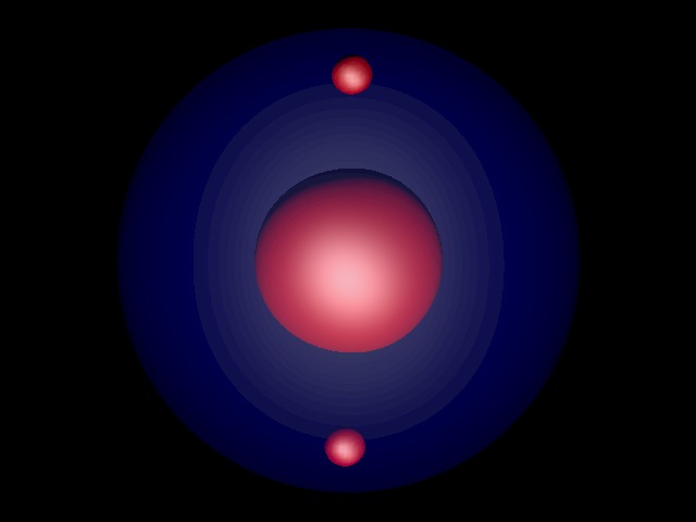
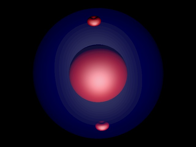
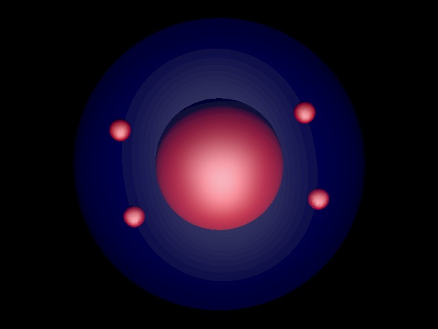
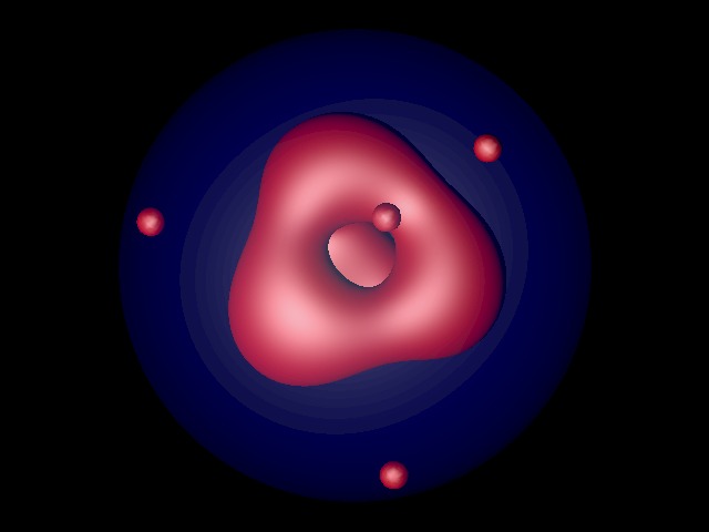
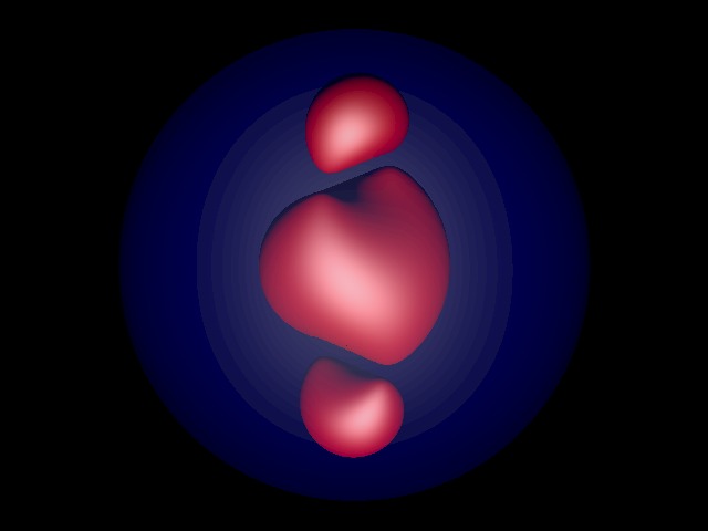
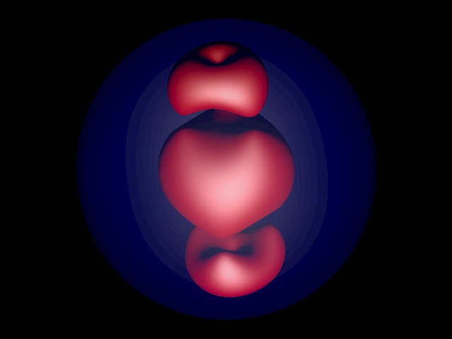
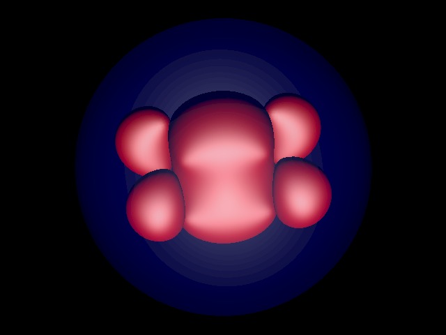
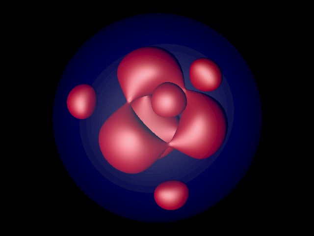
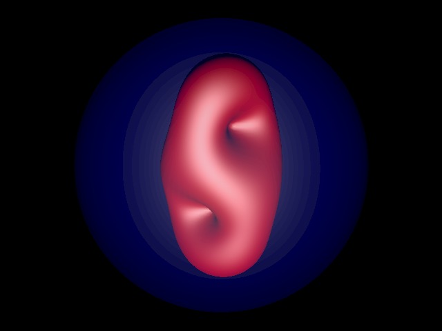
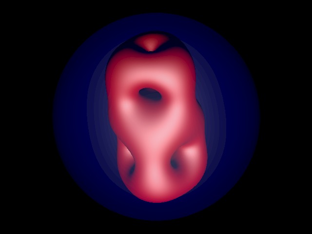
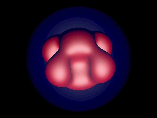
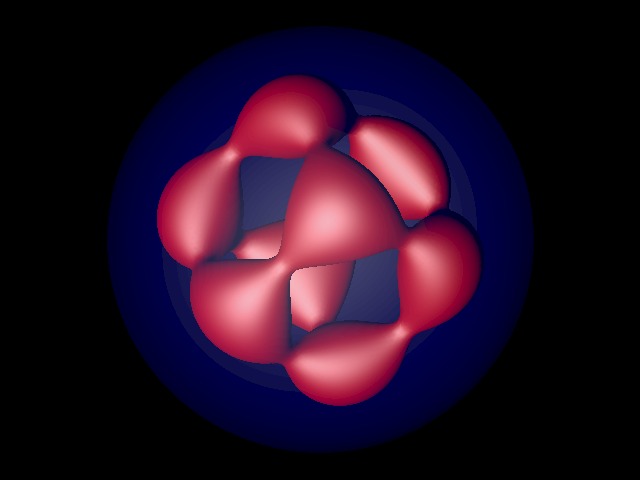
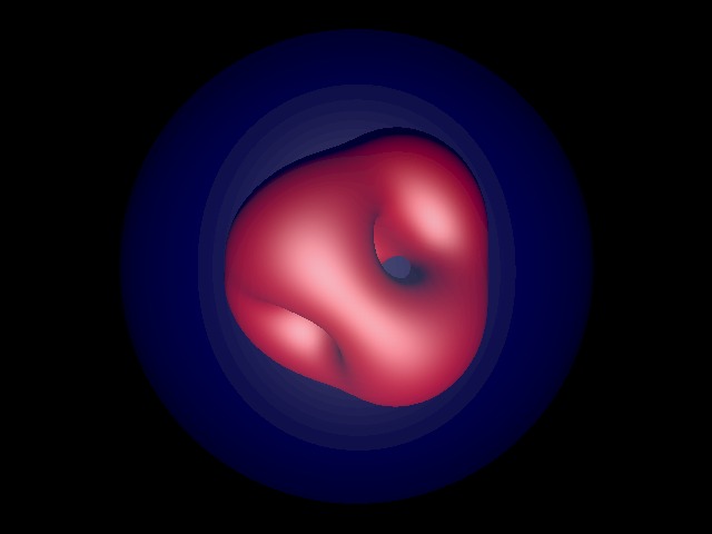
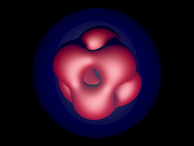
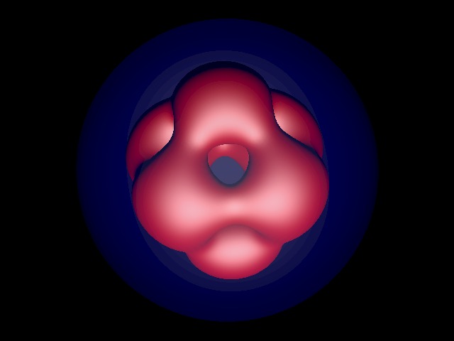
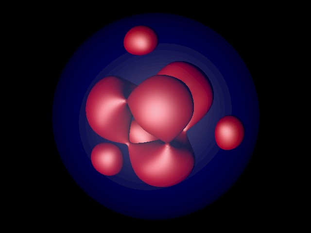
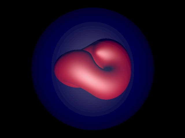
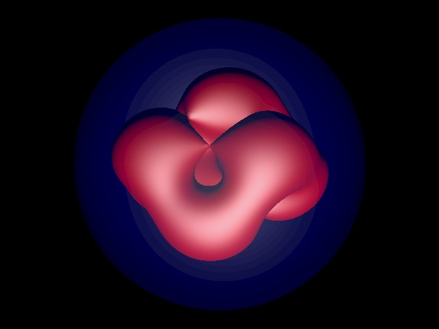
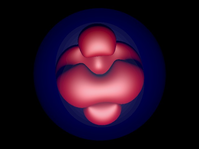
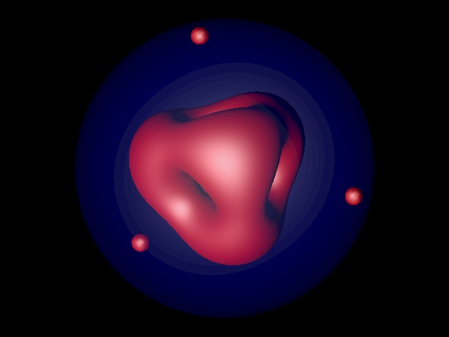
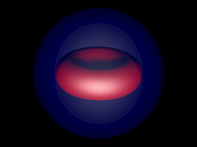
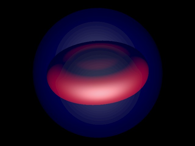
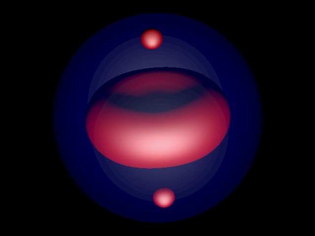
Figure 1: Energy density isosurfaces: first column $D_{2}$ symmetric 3-monopoles, second column $D_{3}$ symmetric 5-monopoles, third column $D_{4}$ symmetric 5-monopoles, fourth column tetrahedrally symmetric 7-monopoles.

5.1 3-monopoles with $D_{2}$ symmetry

This example is of the first type, which is perhaps the most obvious method to construct a symmetric family, since the symmetry of the monopole is simply the symmetry of the points on the sphere corresponding to the positions of the poles. The one-parameter family is given by $a\in(-1,1)$ where we take the four poles

$$\gamma_{0}=\sqrt{\frac{1+a}{1-a}}e^{i\pi/4},\ \gamma_{1}=-\gamma_{0},\ \gamma_{2}=1/\gamma_{0},\ \gamma_{3}=-1/\gamma_{0},$$ (5.1)

with canonical weights, giving an obvious dihedral $D_{2}$ symmetry. The spectral curve is

$$(\eta-\zeta)(\eta^{2}+\zeta^{2}-\frac{4a^{2}}{1-a^{2}}\eta\zeta)+ia(\eta+\zeta)(\eta\zeta+1)(\eta\zeta-1)=0,$$ (5.2)

and is invariant under

$$(\eta,\zeta)\mapsto(-\eta,-\zeta),\qquad\qquad(\eta,\zeta)\mapsto\bigg{(}\frac{1}{\eta},\frac{1}{\zeta}\bigg{)},$$ (5.3)

which generate the $D_{2}$ subgroup of the tetrahedral group (4.3). Note that the change of sign $a\mapsto-a$ is equivalent to the $90^{\circ}$ rotation $(\eta,\zeta)\mapsto(i\eta,i\zeta)$.

The behaviour of the three monopoles as the parameter $a$ is varied can be determined by an examination of the spectral curve (5.2) for particular pertinent values of $a.$ If $a=0$ then (5.2) becomes the axial curve (3.18) with $N=3,$ and if $a=1/\sqrt{3}$ it is the tetrahedral curve (4.2). Given the above comment regarding $a\mapsto-a$ we see that the curve is also tetrahedrally symmetric if $a=-1/\sqrt{3},$ when the dual tetrahedron is obtained. In the limit as $a\to\pm 1$ the spectral curve tends to the curve $(\eta-\zeta)\eta\zeta=0,$ and we see by comparison with (3.4), that this is the product of three stars for monopoles with positions $(X_{1},X_{2},X_{3})$ given by $(0,0,0)$ and $(0,0,\pm 1).$ We therefore find that as $a$ is varied from $-1$ to $1$, two monopoles from infinity approach a monopole at the origin from opposite directions along a line, form the tetrahedral 3-monopole, then the axial 3-monopole, and then separate in the same manner along the same line but with a $90^{\circ}$ rotation about the line.

Using equation (2.5) we have an explicit (though cumbersome) expression for $|\Phi|^{2}$ for the whole family and hence can obtain an explicit form for the energy density by applying the Laplace-Beltrami operator. This process generates the energy density isosurfaces displayed in the first column of Figure 1, which correspond to increasing values of $a\in(-1,0].$ Plots for $a>0$ are not shown since they are simply $90^{\circ}$ rotations of the plots for $a<0.$ The blue sphere in the energy density plots represents the boundary of hyperbolic space and, of course, a monopole appears smaller as it approaches this boundary because of the effect of the metric in the unit ball model of hyperbolic space. This one-parameter family is the hyperbolic analogue of the twisted line scattering of three Euclidean monopoles presented in [20], where the spectral curve is known via a solution of the Nahm equation but the Higgs field and energy density is only available by means of a numerical computation of the Nahm transform.

The rational map for this one-parameter family is obtained using equation (3.17) and is given by

$${\cal R}=\frac{ia(3+a^{2})z^{2}+1-a^{2}}{(1-a^{2})(z^{3}+iaz)},$$ (5.4)

with the manifest $C_{2}$ symmetry ${\cal R}(-z)=-{\cal R}(z).$

5.2 5-monopoles with $D_{3}$ symmetry

The 3-monopole twisted line family of subsection 5.1 includes the tetrahedral 3-monopole and there is a similar 5-monopole twisted line family that includes the octahedral 5-monopole. The Euclidean version of this family was identified in [20] but the associated spectral curves or (numerical) energy density plots have not been investigated. The hyperbolic version can easily be studied in explicit detail using our new approach, with the following results.

The six canonical weight poles are taken to be

$$\gamma_{j}=\sqrt{\frac{1+a}{1-a}}e^{i\pi(1+4j)/6},\quad\gamma_{j+3}=1/\gamma_{j},\quad j=0,1,2,$$ (5.5)

where $a\in(-1,1).$ This yields the spectral curve

$$\eta^{5}-\zeta^{5}-\frac{2ia}{\sqrt{1-a^{2}}}(\eta^{5}\zeta^{3}-\eta^{3}\zeta^{5}+\eta^{2}-\zeta^{2})-\frac{(1+3a^{2})}{(1-a^{2})}(\eta^{4}\zeta-\eta\zeta^{4})+\frac{(1+10a^{2}+5a^{4})}{(1-a^{2})^{2}}(\eta^{3}\zeta^{2}-\eta^{2}\zeta^{3})=0,$$ (5.6)

which is invariant under the $D_{3}$ symmetry generated by

$$(\eta,\zeta)\mapsto(\omega\eta,\omega\zeta),\qquad\qquad(\eta,\zeta)\mapsto\bigg{(}\frac{1}{\eta},\frac{1}{\zeta}\bigg{)},$$ (5.7)

where $\omega=e^{2\pi i/3}.$ There is octahedral symmetry when $a=-\frac{1}{\sqrt{3}}$ and the curve becomes

$$(\eta-\zeta)\big{(}\eta^{4}+\zeta^{4}-2(\eta^{3}\zeta+\eta\zeta^{3})+9\eta^{2}\zeta^{2}+\sqrt{2}i(\eta^{4}\zeta^{3}+\eta^{3}\zeta^{4}+\eta+\zeta)\big{)}=0,$$ (5.8)

which agrees with the earlier octahedral curve (4.7) after a spatial rotation. The replacement $a\mapsto-a$ is equivalent to a rotation through $60^{\circ}$ around the main symmetry axis and the curve (5.6) is axially symmetric if $a=0.$ In the limit $a\to\pm 1$ the curve becomes $(\eta-\zeta)\eta^{2}\zeta^{2}=0,$ which is the product of a star for a 1-monopole at the origin and the curves (3.19) for two axial 2-monopoles at infinity with positions $(X_{1},X_{2},X_{3})=(0,0,\pm 1).$ This twisted line family therefore describes two axial 2-monopoles that approach a single monopole at the origin, from either side of the symmetry axis, form the octahedral 5-monopole, then the axial 5-monopole, with the process then reversing with an accompanying rotation by $60^{\circ}.$ Some selected energy density isosurfaces are presented in the second column of Figure 1, for increasing values of $a\in(-1,0].$

The rational map for this family is

$${\cal R}=\frac{\sqrt{1-a^{2}}-4ia\frac{(1+a^{2})}{(1-a^{2})}z^{3}}{\sqrt{1-a^{2}}z^{5}-2iaz^{2}},$$ (5.9)

with the $C_{3}$ symmetry realized as ${\cal R}(\omega z)={\cal R}(z)/\omega^{2}.$

5.3 5-monopoles with $D_{4}$ symmetry

Our second type of family is perhaps less intuitive then the first type, as it involves fixing the positions of the poles but varying the weights away from their canonical values. As an example we present a one-parameter family of 5-monopoles with $D_{4}$ symmetry that includes the octahedral 5-monopole.

The six poles are placed at the vertices of an octahedron

$$\gamma_{0}=\infty,\ \gamma_{1}=1,\ \gamma_{2}=-1,\ \gamma_{3}=i,\ \gamma_{4}=-i,\ \gamma_{5}=0,$$ (5.10)

so this data is of ’t Hooft form as one of the poles is at $\infty.$ The weights of the remaining five poles are taken to be

$$\lambda_{5}^{2}=1,\qquad\lambda_{1}^{2}=\lambda_{2}^{2}=\lambda_{3}^{2}=\lambda_{4}^{2},$$ (5.11)

with $\lambda_{1}\in(0,\infty)$ the parameter of this family. If $\lambda_{1}=\sqrt{2},$ then all weights are canonical and there is octahedral symmetry, but otherwise the symmetry is broken to $D_{4}$ symmetry.

The spectral curve is

$$(\eta-\zeta)(\eta^{4}\zeta^{4}-\eta^{4}+4\lambda_{1}^{2}\eta^{3}\zeta+4\lambda_{1}^{2}\eta\zeta^{3}-\zeta^{4}+1)=0,$$ (5.12)

and is invariant under

$$(\eta,\zeta)\mapsto(i\eta,i\zeta),\qquad\qquad(\eta,\zeta)\mapsto\bigg{(}\frac{1}{\eta},\frac{1}{\zeta}\bigg{)},$$ (5.13)

which generate the $D_{4}$ symmetry.

If $\lambda_{1}=\sqrt{2}$ then the curve (5.12) reverts to the spectral curve (4.7) of the octahedral 5-monopole. In the limit $\lambda_{1}\to 0$ the curve (5.12) becomes

$$(\eta-\zeta)(\eta^{4}\zeta^{4}-\eta^{4}-\zeta^{4}+1)=0=(\eta-\zeta)\prod_{j=1}^{4}(\eta+i^{j})(\zeta-i^{j})$$ (5.14)

which is the product of stars for five monopoles, with one at the origin $(X_{1},X_{2},X_{3})=(0,0,0)$ and the remaining four monopoles at the boundary of hyperbolic space along the Cartesian axes $(\pm 1,0,0)$ and $(0,\pm 1,0).$ In the opposite limit $\lambda_{1}\to\infty$ the curve becomes

$$\eta\zeta(\eta^{3}-\eta^{2}\zeta+\eta\zeta^{2}-\zeta^{3})=0,$$ (5.15)

where the first two factors describe 1-monopoles at the boundary of hyperbolic space with positions $(0,0,\pm 1)$ and the final factor is the spectral curve of the axial 3-monopole at the origin.

We therefore see that as $\lambda_{1}$ increases through the interval $(0,\infty)$, four 1-monopoles approach from infinity along the Cartesian axes in the plane $X_{3}=0$ and merge with a 1-monopole at the origin to form the octahedral 5-monopole. The octahedral 5-monopole then splits to produce two 1-monopoles moving in opposite directions along the $X_{3}$-axis, leaving behind the axial 3-monopole. Corresponding energy density isosurfaces are displayed in the third column of Figure 1. Note that, as with some of the other energy density isosurfaces presented in this paper, we often slightly rotate the image to obtain an improved viewing angle, so for example the $X_{3}$-axis may not be exactly aligned with the vertical, although the images within each column have the same viewing angle.

The rational map for this one-parameter family is

$${\cal R}=\frac{(4\lambda_{1}^{2}+1)z^{4}-1}{z^{5}-z},$$ (5.16)

with the clear $C_{4}$ symmetry ${\cal R}(iz)=-i{\cal R}(z).$

5.4 7-monopoles with tetrahedral symmetry

Our next example of a family of the second type illustrates the fact that dihedral symmetry, although convenient for producing one-parameter families, is certainly not the only possibility. In this subsection, we construct a one-parameter family of 7-monopoles by imposing tetrahedral symmetry.

The eight poles are taken to be the roots of the Klein polynomial (4.9) for the face centres of the octahedron (or equivalently the vertices of the cube). Explicitly, we label the poles as

$$\gamma_{0}=\frac{1+i}{\sqrt{3}+1},\ \gamma_{1}=-\gamma_{0},\ \gamma_{2}=\gamma_{0}^{-1},\ \gamma_{3}=-\gamma_{0}^{-1},\ \gamma_{4}=\frac{1-i}{\sqrt{3}+1},\ \gamma_{5}=-\gamma_{4},\ \gamma_{6}=\gamma_{4}^{-1},\ \gamma_{7}=-\gamma_{4}^{-1},$$ (5.17)

and take $\lambda_{j}^{2}$ to be canonical weights for $j=0,1,2,3$ but $\mu^{2}$ times the canonical weights for $j=4,5,6,7.$ The one-parameter family is given by $\mu\in(0,\infty)$ with the resulting spectral curve taking the form

$$\bigg{(}(\eta-\zeta)^{3}+\frac{i}{\sqrt{3}}(\eta+\zeta)(\eta\zeta+1)(\eta\zeta-1)\bigg{)}\prod_{j=4}^{7}(\eta\zeta\bar{\gamma}_{j}+\zeta-\eta|\gamma_{j}|^{2}-\gamma_{j})$$ (5.18)

$$+\mu^{2}\bigg{(}(\eta-\zeta)^{3}-\frac{i}{\sqrt{3}}(\eta+\zeta)(\eta\zeta+1)(\eta\zeta-1)\bigg{)}\prod_{j=0}^{3}(\eta\zeta\bar{\gamma}_{j}+\zeta-\eta|\gamma_{j}|^{2}-\gamma_{j})=0,$$

where the first term is the product of the tetrahedral 3-monopole curve (4.2) and four stars for monopoles on the sphere at infinity on the vertices of the dual tetrahedron. The second term is $\mu^{2}$ times the first term after the replacement $(\eta,\zeta)\mapsto(i\eta,i\zeta).$ The transformation $\mu\mapsto\mu^{-1}$ is therefore equivalent to a rotation by $90^{\circ}$ around the $X_{3}$-axis.

If $\mu=1$ then the tetrahedral symmetry is enhanced to cubic symmetry, as there are eight poles with canonical weights on the vertices of a cube. $N=7$ is not the lowest value of $N$ for which there is a hyperbolic monopole with cubic symmetry. The lowest value is $N=4$ and the spectral curve can be found in [10] with the explicit Higgs field derived in [2] using the ADHM construction with circle invariance. However, this cubic 4-monopole is clearly not within the JNR class, as five points cannot be placed on a sphere with cubic symmetry.

We see from the above spectral curve that as $\mu$ increases through the interval $(0,\infty),$ four monopoles approach from infinity towards the face centers of the tetrahedral 3-monopole. The monopoles then merge to form a cubic 7-monopole which subsequently splits to leave the dual tetrahedral 3-monopole with four monopoles receding from the face centres towards infinity. Energy density isosurfaces are displayed in the fourth column of Figure 1 for increasing values of $\mu.$

For values of $\mu$ around that associated with the second image in the fourth column of Figure 1 (or equivalently the fourth image in this column), we may view this solution as a prototype hyperbolic analogue of the multi-shell Euclidean monopoles suggested in [21] within the magnetic bag approximation.

The rational map for the family is

$${\cal R}=\frac{(1-\mu^{4})(5z^{6}-z^{2})-i\sqrt{3}(1+\mu^{2})^{2}(11z^{4}+1)}{i\sqrt{3}(1+\mu^{2})^{2}(z^{7}+3z^{3})+(1-\mu^{4})(5z^{5}+z)},$$ (5.19)

with the evident $C_{2}$ symmetry ${\cal R}(-z)=-{\cal R}(z).$ For the cubic $\mu=1$ case the map simplifies to

$${\cal R}=\frac{11z^{4}+1}{z^{7}+3z^{3}},$$ (5.20)

with the manifest $C_{4}$ symmetry ${\cal R}(iz)=i{\cal R}(z).$

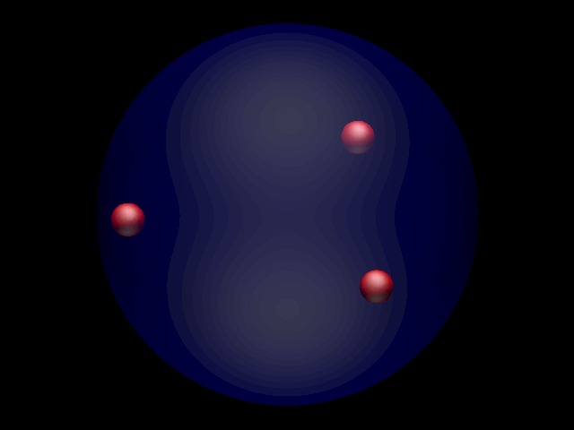
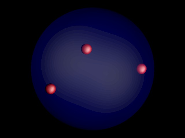
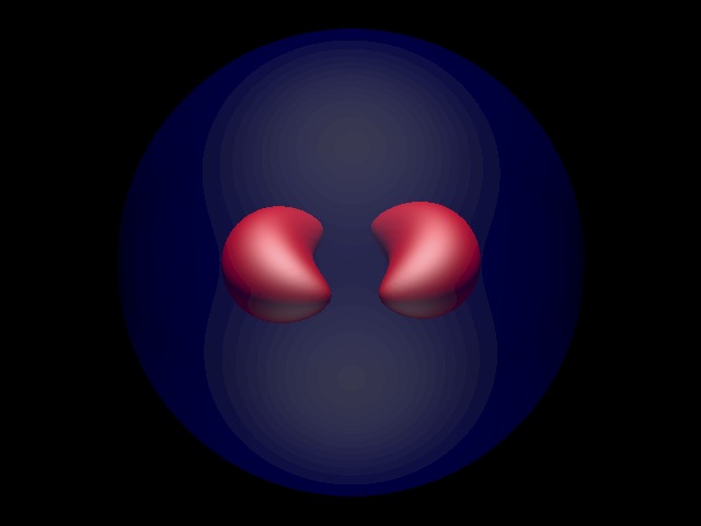
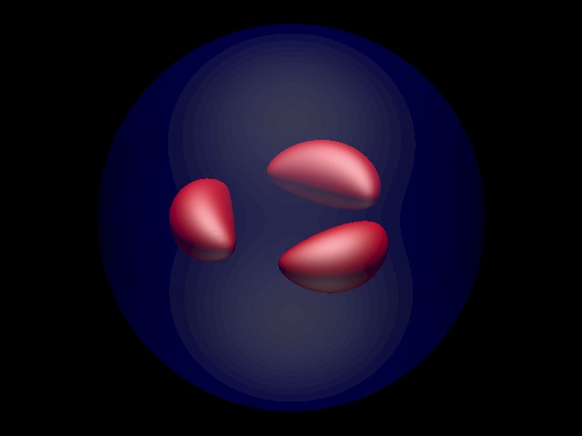
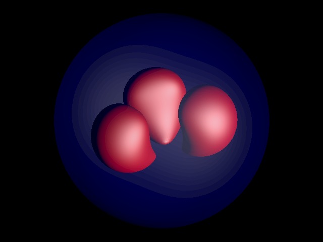
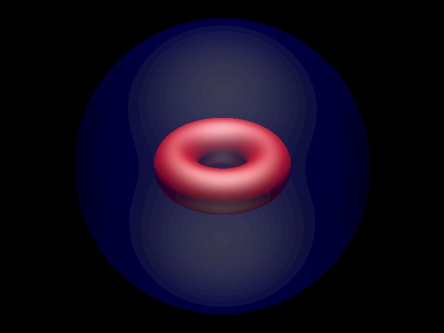
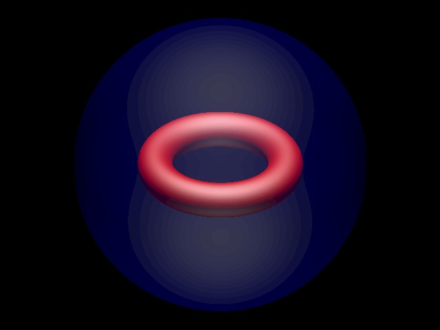
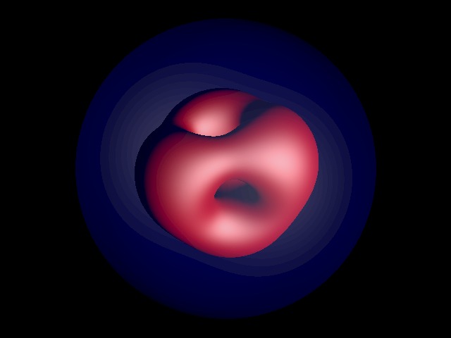
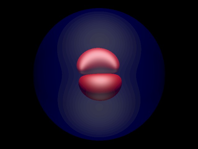
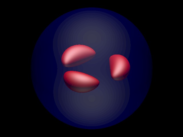
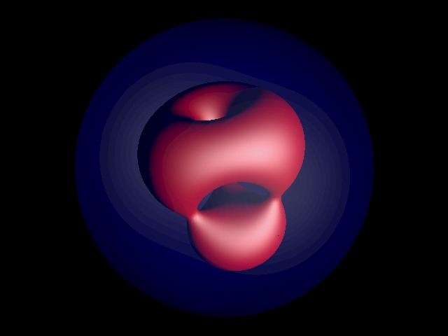
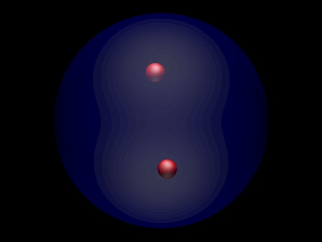
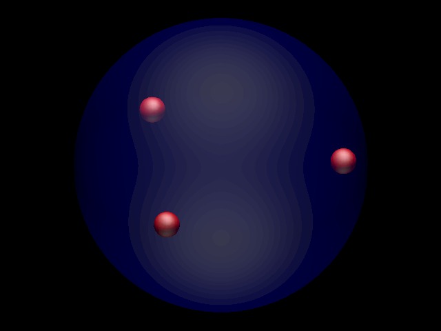
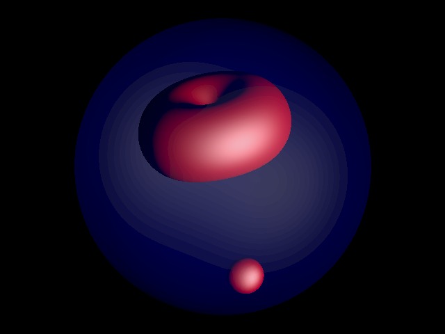
Figure 2: Energy density isosurfaces: first column $D_{2}$ symmetric 2-monopoles, second column $D_{3}$ symmetric 3-monopoles, third column $C_{3}$ symmetric 3-monopoles.

5.5 2-monopoles with $D_{2}$ symmetry

Our first example of a family of type three, where the positions of the poles vary together with the (generically) non-canonical weights, is a one-parameter family of $D_{2}$ symmetric 2-monopoles. Although this is perhaps the simplest family of multi-monopoles, and was studied in [2] using the ADHM formalism, its analysis in terms of the JNR approach is a little subtle, and is therefore worth presenting.

It is not immediately obvious how to place three poles and select their weights so that there is $D_{2}$ symmetry. Clearly this requires exploiting the degeneracy that arises when all poles lie on a circle, which we take to be the unit circle in the plane $X_{3}=0.$ Imposing the subgroup $C_{2}$ symmetry given by a rotation by $180^{\circ}$ around the $X_{1}$-axis is straightforward, as one of the poles can be placed on the $X_{1}$-axis with the two remaining poles placed symmetrically about the axis with equal weights. Explicitly, let $a\in(-1,1)$ be the parameter of the family and set

$$\gamma_{0}=1,\ \ \gamma_{1}=\frac{a-1}{2}+\frac{i}{2}\sqrt{3+2a-a^{2}},\ \ \gamma_{2}=\gamma_{1}^{-1},\ \ \lambda_{1}^{2}=\lambda_{2}^{2}=1,$$ (5.21)

with the weight $\lambda_{0}^{2}$ undetermined for the moment.

The spectral curve is

$$\frac{(\lambda_{0}^{2}+a-1)}{(2+\lambda_{0}^{2})}(\eta^{2}\zeta^{2}+1)+\frac{(\lambda_{0}^{2}-a\lambda_{0}^{2}-a-1)}{(2+\lambda_{0}^{2})}(\eta^{2}\zeta-\eta\zeta^{2}-\eta+\zeta)+\eta^{2}+\zeta^{2}-\frac{(2+2a+\lambda_{0}^{2}(1-a)^{2})}{(2+\lambda_{0}^{2})}\eta\zeta=0,$$ (5.22)

and is invariant under the $C_{2}$ symmetry $(\eta,\zeta)\mapsto({\eta}^{-1},{\zeta}^{-1}).$ This $C_{2}$ symmetry is extended to $D_{2}$ symmetry by requiring invariance of the spectral curve (5.22) under the additional generator $(\eta,\zeta)\mapsto(-\eta,-\zeta).$ This extra symmetry requires that the coefficient $c_{ij}$ vanishes unless $(i+j)\,\mbox{mod}\,2=0.$ This is satisfied providing

$$\lambda_{0}^{2}=\frac{1+a}{1-a},$$ (5.23)

which yields the required $D_{2}$ invariant spectral curve

$$\eta^{2}+\zeta^{2}+a(\eta^{2}\zeta^{2}+1)+(a^{2}-1)\eta\zeta=0.$$ (5.24)

We see from (5.24) that $a\mapsto-a$ is equivalent to the $90^{\circ}$ rotation $(\eta,\zeta)\mapsto(i\eta,i\zeta),$ and furthermore the axial 2-monopole curve is recovered by setting $a=0.$

The boundary of hyperbolic space intersects the plane $X_{3}=0$ in the circle given by $(X_{1},X_{2},X_{3})=(\cos\theta,\sin\theta,0)$, and from (3.4) a monopole at this position corresponds to the star

$$(\eta+e^{i\theta})(\zeta-e^{i\theta})=0.$$ (5.25)

In the limit $a\to-1$ the curve (5.24) becomes the product of two stars

$$(\eta+1)(\zeta-1)(\eta-1)(\zeta+1)=0$$ (5.26)

for monopoles with positions $(\pm 1,0,0).$ Therefore as $a$ increases through $(-1,1)$ the two monopoles approach along the $X_{1}$-axis, merge to form the axially symmetric 2-monopole, and separate along the $X_{2}$-axis. This is the hyperbolic analogue of the famous right angle scattering of two Euclidean monopoles discovered by Atiyah and Hitchin [22]. Energy density isosurfaces are displayed for increasing values of $a$ in the first column of Figure 2.

The rational map for this family is

$${\cal R}=\frac{1-a^{2}}{z^{2}+a},$$ (5.27)

with the manifest $C_{2}$ symmetry ${\cal R}(-z)={\cal R}(z).$

5.6 3-monopoles with $D_{3}$ symmetry

The one-parameter family of $D_{2}$ symmetric 2-monopoles, studied in the previous subsection, has a generalization to a one-parameter family of $D_{N}$ symmetric $N$-monopoles. The $N$ monopoles are located on the vertices of a contracting regular $N$-gon, merge to form the axial $N$-monopole, and then separate on the vertices of an expanding regular $N$-gon, that is obtained from the incoming polygon by a rotation through $180^{\circ}/N.$

We illustrate this generalization by presenting the result for $N=3$. The four poles are again taken to lie on the unit circle, but this time two of the poles are placed on the $X_{1}$-axis to achieve the $C_{2}$ symmetry given by a rotation by $180^{\circ}$ around the $X_{1}$-axis. As before, the two remaining poles are placed symmetrically about this axis with equal weights. In detail, the parameter is $a\in(-1,1)$ and the poles and weights are

$$\gamma_{0}=1,\ \gamma_{1}=-1,\ \gamma_{2}=\frac{1}{2}(a+i\sqrt{4-a^{2}}),\ \gamma_{3}=\gamma_{2}^{-1},\ \lambda_{0}^{2}=1,\ \lambda_{2}^{2}=\lambda_{3}^{2},$$ (5.28)

with $\lambda_{1}$ and $\lambda_{2}$ yet to be determined. The $D_{3}$ symmetry is obtained by demanding that the spectral curve is invariant under the additional $C_{3}$ symmetry $(\eta,\zeta)\mapsto(\omega\eta,\omega\zeta),$ where $\omega=e^{2i\pi/3}.$ This results in the requirement that $c_{ij}=0$ if $(i+j)\,\mbox{mod}\,3\neq 0,$ which gives

$$\lambda_{1}^{2}=\frac{(1-a)(2-a)}{(1+a)(2+a)},\qquad\lambda_{2}^{2}=\frac{2(1-a)}{(2+a)}.$$ (5.29)

The one-parameter family of $D_{3}$ symmetric spectral curves is then

$$\eta^{3}-\zeta^{3}+a(\eta^{3}\zeta^{3}-1)+(a^{2}-1)(\eta^{2}\zeta-\eta\zeta^{2})=0,$$ (5.30)

which satisfies all the properties expected of this family, as described at the start of this subsection. Some energy density isosurfaces are displayed in the second column of Figure 2 for increasing values of $a\in(-1,1).$

The rational map is

$${\cal R}=\frac{1-a^{2}}{z^{3}+a},$$ (5.31)

being the obvious generalization of (5.27). For larger values of $N$ the procedure follows the same process as in this subsection and the previous one, with one pole on the $X_{1}$-axis if $N$ is even and two if $N$ is odd. The remaining poles are placed symmetrically in pairs around the unit circle, with equal weights to attain the $C_{2}$ symmetry, with the weights then determined by applying an additional $C_{N}$ generator to enforce the full $D_{N}$ symmetry.

5.7 3-monopoles with $C_{3}$ symmetry

Our final example illustrates a phenomenon that appears if cyclic symmetry is imposed, rather than dihedral symmetry. Imposing cyclic symmetry will produce more than a one-parameter family, as there will be an additional degree of freedom associated with a translation of the whole configuration along the symmetry axis.

In Euclidean space, the motion of $N$ monopoles has a natural decomposition into a trivial motion of the centre of mass of the configuration and a non-trivial relative motion between monopoles. In terms of the moduli space approximation, this allows (without loss of generality) a restriction to centered monopoles, in which the centre of mass is fixed at the origin. In hyperbolic space the situation is not so simple, since there is no definition of the centre of mass (even for point particles) that has all the properties that exist in the Euclidean setting. Fortunately there is a definition [9] for a hyperbolic monopole to be centered, so we will apply this definition to restrict to a one-parameter family.

The definition introduced in [9] for a centered hyperbolic monopole is by no means obvious and relies upon the use of yet another holomorphic object associated with a hyperbolic monopole, namely a holomorphic sphere. This is a holomorphic map from $\mathbb{CP}^{1}$ to $\mathbb{CP}^{N}$, and the action of the isometries of hyperbolic space induces a moment map whose zero set can be used to define conditions for a spectral curve to correspond to a centered hyperbolic monopole. These conditions map to simple linear relations between the coefficients $c_{ij}$ in the spectral curve. All the spectral curves that we have presented so far obey these centered conditions, as a result of the symmetries that we have imposed. In particular, rewriting the results of [9] in terms of these linear relations we find that a 3-monopole is centered if the coefficients of its spectral curve satisfy

$$9c_{30}-c_{21}-c_{12}+9c_{03}=3c_{31}-2c_{22}+3c_{13}=0.$$ (5.32)

We shall make use of this condition shortly.

The cyclic example we consider is $C_{3}$ symmetric 3-monopoles obtained from the following choice of four poles,

$$\gamma_{0}=0,\qquad\gamma_{j}=\sqrt{\frac{1+a}{1-a}}\omega^{j}\quad\mbox{ for }j=1,2,3,$$ (5.33)

where $\omega=e^{2\pi i/3}$ and $a\in(-1,1)$ is the free parameter. The weights $\lambda_{j}^{2}$ are canonical for $j=1,2,3$ but $\lambda_{0}^{2}$ is free for the moment. This yields the two-parameter family of $C_{3}$ symmetric spectral curves

$$\lambda_{0}^{2}\sqrt{\frac{1+a}{1-a}}(\eta^{3}\zeta^{3}-1)-\lambda_{0}^{2}\frac{(1+a)^{2}}{(1-a)^{2}}\eta^{3}+\frac{6(1+a)}{(1-a)^{2}}\eta^{2}\zeta-\frac{6}{(1-a)}\eta\zeta^{2}+\frac{(6+\lambda_{0}^{2}-a\lambda_{0}^{2})}{(1+a)}\zeta^{3}=0,$$ (5.34)

invariant under the symmetry $(\eta,\zeta)\mapsto(\omega\eta,\omega\zeta).$

We now reduce this two-parameter family to a one-parameter family by imposing the centered condition (5.32), which determines the weight to be

$$\lambda_{0}^{2}=\frac{9-20a+7a^{2}}{3a(3+a^{2})}.$$ (5.35)

The requirement that $\lambda_{0}^{2}>0$ imposes the restriction $a\in(0,a_{\star})$, where $a_{\star}=(10-\sqrt{37})/7.$

Substituting (5.35) into (5.34) produces the centered spectral curve

$$\sqrt{\frac{1+a}{1-a}}(\eta^{3}\zeta^{3}-1)-\frac{(1+a)^{2}}{(1-a)^{2}}\eta^{3}+\frac{18a(3+a^{2})(\eta^{2}\zeta(1+a)-\eta\zeta^{2}(1-a))}{(1-a)^{2}(9-20a+7a^{2})}+\frac{(9+16a+11a^{2})}{(9-20a+7a^{2})}\zeta^{3}=0.$$ (5.36)

The curve has tetrahedral symmetry if $a=\frac{1}{3}$ when it becomes

$$\sqrt{2}\eta^{3}\zeta^{3}-4\eta^{3}+18\eta^{2}\zeta-9\eta\zeta^{2}+5\zeta^{3}-\sqrt{2}=0,$$ (5.37)

with the extra $C_{2}$ symmetry

$$(\eta,\zeta)\mapsto\bigg{(}\frac{\sqrt{2}-\eta}{\sqrt{2}\eta+1},\frac{\sqrt{2}-\zeta}{\sqrt{2}\zeta+1}\bigg{)}.$$ (5.38)

This tetrahedral curve is equal to the earlier tetrahedral curve (4.2) after a suitable rotation. In the limit $a\to 0$ the curve is a product of stars

$$\eta^{3}\zeta^{3}-\eta^{3}+\zeta^{3}-1=0=\prod_{j=1}^{3}(\eta+\omega^{j})(\zeta-\omega^{j})$$ (5.39)

for three monopoles on the vertices of an equilateral triangle in the plane $X_{3}=0$ at the boundary of hyperbolic space. In the limit $a\to a_{\star}$ the curve becomes

$$\zeta\bigg{(}(1+b)^{4}\eta^{2}+(1-b)^{4}\zeta^{2}-{(1-b^{2})^{2}}\eta\zeta\bigg{)}=0,$$ (5.40)

where $b$ is given by the relation $a_{\star}=2b/(1+b^{2}),$ so $b=(7-2\sqrt{5\sqrt{37}-22})/(10-\sqrt{37})\approx 0.3.$ This curve is the product of a star for a monopole at $(0,0,-1)$ and the curve (3.19) for an axial 2-monopole at $(0,0,b).$ The interesting new phenomenon here is that the single monopole is at infinity when the axial 2-monopole is at a finite distance from the origin, despite the fact that the total configuration is centered. This contrasts with the Euclidean situation, where an $N$-monopole cannot be centered if it consists of two clusters with only one cluster at infinity, as is self-evident from the properties of the centre of mass in Euclidean space.

A possible physical understanding of this new phenomenon in hyperbolic space is that the condition for a hyperbolic monopole to be centered should be similar to a requirement that the magnetic field on the sphere at infinity has a vanishing dipole. A definition of this sort would be quite natural, given that the abelian magnetic field on the sphere at infinity completely determines the monopole [4]. A single monopole has a finite dipole even as its position tends to the sphere at infinity in hyperbolic space, so this can indeed be cancelled by a non-zero dipole of a cluster in the interior of hyperbolic space. At the moment this is nothing more than an attempt at a potential physical understanding of this surprising phenomenon, but it at least suggests why the result is not unreasonable.

In summary, the one-parameter family described in this subsection consists of three monopoles that approach on the vertices of a contracting triangle, merge to form the tetrahedral 3-monopole, which then splits into a single monopole that travels down the symmetry axis of the triangle, leaving an axial 2-monopole at a finite distance up the symmetry axis. A selection of the corresponding energy density isosurfaces are displayed in the third column of Figure 2. This process is a hyperbolic analogue of the $C_{3}$ symmetric scattering of three Euclidean monopoles, for which similar energy density isosurfaces can be seen in [23]; except that the axial 2-monopole continues to travel along the axis. These Euclidean results involve a numerical computation of the relevant solution of the Nahm equation, as the associated genus four curve is the Galois cover of a genus two curve (rather than an elliptic curve). Progress has been made in computing the spectral curve for this Euclidean case [24], but it is significantly more complicated than the hyperbolic spectral curve (5.36).

The rational map for the centered $C_{3}$ symmetric 3-monopole family is

$${\cal R}=\frac{18a(3+a^{2})\sqrt{\frac{1+a}{1-a}}z}{(1-a)(11a^{2}+16a+9)z^{3}-\sqrt{1-a^{2}}(7a^{2}-20a+9)},$$ (5.41)

with the symmetry realized as ${\cal R}(\omega z)=\omega{\cal R}(z)$. Note that this is a different realization of the $C_{3}$ symmetry than for the rational map (5.31) of the $D_{3}$ symmetric 3-monopole of the previous subsection, where ${\cal R}(\omega z)={\cal R}(z).$ Although both families involve three monopoles on the vertices of a contracting triangle, the subsequent different configurations are a result of different arrangements of the relative phases, which are captured by the above rational map realizations of the $C_{3}$ symmetry.

6 A metric on the space of JNR data

Monopole dynamics in Euclidean space can be approximated by geodesic motion on the monopole moduli space equipped with the natural $L^{2}$ metric [19]. However, the $L^{2}$ metric on the moduli space of hyperbolic monopoles is infinite, so this approximation is unavailable for studying the dynamics of hyperbolic monopoles. An alternative approach is to use the fact that a hyperbolic monopole is uniquely determined by its abelian magnetic field on the boundary of hyperbolic space, and the associated abelian connection can be used to define a finite metric on the monopole moduli space [4]. This metric is invariant under the isometries of hyperbolic space, and in the case of a single monopole the moduli space equipped with this metric is simply hyperbolic space itself. Applying the moduli space approximation with this metric therefore yields the natural result that a slowly moving single hyperbolic monopole follows a geodesic in hyperbolic space.

In this section we provide a simple integral formula for the above metric restricted to the space of JNR data and illustrate its application by explicit computation to confirm that hyperbolic space is obtained as the moduli space for a single monopole.

To present the metric it is most convenient to use the upper half space model of hyperbolic space, where the boundary is given by $r=0$ and we set $z=x_{1}+ix_{2}$ to be the complex coordinate on the boundary. As shown in [9], the required connection on the sphere at infinity can be written in terms of a hermitian metric obtained by evaluating the spectral curve on the antidiagonal. Explicitly, the abelian connection ${\cal A}_{z}=\frac{1}{2}({\cal A}_{1}-i{\cal A}_{2})$ is given in terms of the hermitian metric $h(z,\bar{z})$ by

$${\cal A}_{z}=\frac{1}{2}\partial_{z}\log h,$$ (6.1)

where $h(z,\bar{z})$ is the polynomial in $z$ and $\bar{z}$ obtained as $\bar{z}^{N}$ times the spectral curve evaluated on the antidiagonal $\zeta=z$ and $\eta=-1/\bar{z}.$ Using (3.14) gives the hermitian metric in terms of the JNR data as

$$h(z,\bar{z})=\sum_{j=0}^{N}\lambda_{j}^{2}\mathop{\prod_{k=0}^{N}}_{k\neq j}|z-\gamma_{k}|^{2}=\psi|_{r=0}\prod_{k=0}^{N}|z-\gamma_{k}|^{2}.$$ (6.2)

Let $t_{\mu}$ for $\mu=1,\ldots,\mbox{dim}({\mathbb{M}}^{\mbox{\tiny{JNR}}}_{N})$ be real independent coordinates on the JNR moduli space. The metric is the $L^{2}$ metric of the abelian connection

$$g_{\mu\nu}=K\int\frac{\partial{\cal A}_{i}}{\partial t_{\mu}}\,\frac{\partial{\cal A}_{i}}{\partial t_{\nu}}\,\,d^{2}x=K\int\bigg{(}\frac{\partial}{\partial t_{\mu}}\bigg{(}\frac{\partial_{i}h}{h}\bigg{)}\bigg{)}\bigg{(}\frac{\partial}{\partial t_{\nu}}\bigg{(}\frac{\partial_{i}h}{h}\bigg{)}\bigg{)}\,d^{2}x,$$ (6.3)

where $K$ is a normalization constant.

As an example, consider the case $N=1,$ where the three real independent coordinates may be taken to be those in the ’t Hooft data, that is, $t_{1}+it_{2}=\gamma_{1}$ and $t_{3}=\lambda_{1}.$ The hermitian metric is then

$$h=|z-\gamma_{1}|^{2}\bigg{(}1+\frac{\lambda_{1}^{2}}{|z-\gamma_{1}|^{2}}\bigg{)}=t_{3}^{2}+(x_{1}-t_{1})^{2}+(x_{2}-t_{2}^{2}),$$ (6.4)

and the above formula, with normalization constant $K=3/(8\pi)$, gives the moduli space metric

$$g_{\mu\nu}dt_{\mu}dt_{\nu}=\frac{dt_{1}^{2}+dt_{2}^{2}+dt_{3}^{2}}{t_{3}^{2}}.$$ (6.5)

As advertised, this is indeed the metric of hyperbolic space, in upper half space coordinates.

The moduli space of inversion symmetric hyperbolic 2-monopoles is four-dimensional and is obtained from the action of $SO(3)$ on the one-parameter family of $D_{2}$ symmetric 2-monopoles described earlier. It would be interesting to use the above approach to compute the metric on this moduli space and to compare with both the Atiyah-Hitchin metric for Euclidean 2-monopoles and Hitchin’s metric, with $k=6$ in the notation of [25], which is an algebraic metric on the spectral curves of precisely these hyperbolic 2-monopoles.

As the moduli space metric is invariant under $SO(3)$ spatial rotations then the one-parameter dihedral families discussed in the previous section, being obtained as fixed point sets of a finite subgroup of this $SO(3)$ action, are automatically geodesics with respect to this metric. This relies on the fact that, for the examples considered, there are no hyperbolic monopoles with the given symmetry and charge that lie outside the JNR ansatz, which follows from known results on the dimensions of spaces of symmetric Euclidean monopoles.

7 Conclusion

For a specific relation between the curvature of hyperbolic space and the magnitude of the Higgs field at infinity, we have been able to obtain a complete description of a large class of hyperbolic $N$-monopoles. We have presented simple explicit formulae for the spectral curve and the rational map, in terms of free data given by $N+1$ points on the sphere together with positive real weights. This complements recent work that provided an explicit formula for the Higgs field in terms of the same data. A number of symmetric examples have been presented, including one-parameter families that are hyperbolic analogues of geodesics that describe Euclidean monopole scattering. We have derived an integral expression for an interesting metric on the space of this data and in future work we plan to investigate this aspect further.

Appendix A Appendix

In this appendix we prove the rational map formula (3.17) directly using the definition (3.15) together with the ADHM matrix (3.9) and the change of basis matrices given by (3.11) and (3.12).

The proof involves a formal expansion in $z^{-1}$. We define the coefficients $q_{I}$ and $Q_{I}$ by

$$L(z-M)^{-1}L^{t}=\sum_{I=1}^{\infty}q_{I}z^{-I},$$ (A.1)

$$\left\{\sum^{N}_{i=0}\sum^{N}_{j=i+1}\lambda_{i}^{2}\lambda_{j}^{2}(\gamma_{i}-\gamma_{j})^{2}\prod^{N}_{\begin{subarray}{c}k=0\\ k\neq i,j\end{subarray}}(z-\gamma_{k})\right\}/\left\{\left(\sum^{N}_{i=0}\lambda_{i}^{2}\right)\left(\sum^{N}_{j=0}\lambda_{j}^{2}\prod^{N}_{\begin{subarray}{c}k=0\\ k\neq j\end{subarray}}(z-\gamma_{k})\right)\right\}=\sum_{I=1}^{\infty}Q_{I}z^{-I}.$$ (A.2)

The prove the rational map formula we need to show that $q_{I}=Q_{I},$ which we accomplish by proving that both sets of coefficients satisfy the same inductive relation, together with $q_{1}=Q_{1}$.

To begin, we expand the left hand side of (A.1) to give

$$q_{I}=LM^{I-1}L^{t}.$$ (A.3)

From the $(N+1)\times(N+1)$ matrix $S$, given by (3.12), we define the $N\times(N+1)$ matrix $S^{\prime}$ by removing the top row of $S$. Furthermore, we define this removed row to be $S^{\prime\prime}$. With this decomposition of $S$ and the corresponding decomposition (3.6) of the ADHM matrix, equation (3.9) becomes

$$L=S^{\prime\prime}\Gamma V\quad\textrm{ and }\quad M=S^{\prime}\Gamma V,$$ (A.4)

and therefore

$$q_{I+1}=LM^{I}L^{t}=S^{\prime\prime}\Gamma(VS^{\prime}\Gamma)^{I}VV^{t}\Gamma^{t}(S^{\prime\prime})^{t}.$$ (A.5)

Using the fact that $S$ is an orthogonal matrix, it is easy to show that

$$VS^{\prime}=\frac{1}{\lambda_{0}}(U^{t}-(S^{\prime\prime\prime})^{t}S^{\prime\prime})\quad\textrm{ and }\quad VV^{t}=\frac{1}{\lambda_{0}^{2}}(1-(S^{\prime\prime\prime})^{t}S^{\prime\prime\prime}),$$ (A.6)

where $U$ is the $(N+1)\times N$ matrix obtained from the $N\times N$ identity matrix by adding an extra top row of zeros, and we have defined the $N$-component row vector $S^{\prime\prime\prime}$ by $(S^{\prime\prime\prime})_{i}=(S^{\prime\prime})_{i+1}$. Note that

$$q_{I+1} =S^{\prime\prime}\Gamma\left(\frac{1}{\lambda_{0}}(U^{t}-(S^{\prime\prime\prime})^{t}S^{\prime\prime})\Gamma\right)(VS^{\prime}\Gamma)^{I-1}VV^{t}\Gamma^{t}(S^{\prime\prime})^{t}$$

$$=\frac{1}{\lambda_{0}}S^{\prime\prime}\Gamma U^{t}\Gamma(VS^{\prime}\Gamma)^{I-1}VV^{t}\Gamma^{t}(S^{\prime\prime})^{t}-\frac{1}{\lambda_{0}}(S^{\prime\prime}\Gamma(S^{\prime\prime\prime})^{t})q_{I}.$$ (A.7)

Continuing inductively, after some calculation, one finds that

$$q_{I}=\sum^{I-1}_{J=1}a_{J}q_{I-J}+b_{I},$$ (A.8)

where we have introduced

$$a_{I}=-\frac{1}{\lambda_{0}^{I}}S^{\prime\prime}\Gamma(U^{t}\Gamma)^{I-1}(S^{\prime\prime\prime})^{t}\quad\mbox{ and }\quad b_{I}=\frac{1}{\lambda_{0}^{I-1}}S^{\prime\prime}\Gamma(U^{t}\Gamma)^{I-1}VV^{t}\Gamma^{t}(S^{\prime\prime})^{t}.$$ (A.9)

Since $U^{t}\Gamma$ is diagonal, $a_{I}$ and $b_{I}$ can be calculated to be

$$a_{I}=-p_{N}^{2}\sum^{N}_{j=1}\lambda_{j}^{2}\gamma_{j}^{I-1}(\gamma_{j}-\gamma_{0}),$$ (A.10)

$$b_{I}=\left\{\left(\sum^{N}_{j=1}\lambda_{j}^{2}\gamma_{j}^{I-1}(\gamma_{j}-\gamma_{0})^{2}\right)-p_{N}^{2}\left(\sum^{N}_{j=1}\lambda_{j}^{2}\gamma_{j}^{I-1}(\gamma_{j}-\gamma_{0})\right)\left(\sum^{N}_{k=1}\lambda_{k}^{2}(\gamma_{k}-\gamma_{0})\right)\right\}p_{N}^{2}.$$ (A.11)

As the rational map is invariant under permutations of the poles and weights then the coefficients $q_{I}$ must be too. Taking (A.8), exchanging $(\gamma_{0},\lambda_{0})$ with $(\gamma_{k},\lambda_{k})$ and summing over $k$ from 0 to $N$ yields, after a long but straightforward manipulation,

$$(N+1)q_{I}=\sum^{I-1}_{J=1}\alpha_{J}q_{I-J}+\beta_{I},$$ (A.12)

where

$$\alpha_{I}=-p_{N}^{2}\sum^{N}_{j=0}\sum^{N}_{k=0}\lambda_{j}^{2}\gamma_{j}^{I-1}\left(\gamma_{j}-\gamma_{k}\right),$$ (A.13)

and

$$\beta_{I}=p_{N}^{4}\sum^{N}_{j=0}\sum^{N}_{k=j+1}\lambda_{j}^{2}\lambda_{k}^{2}(\gamma_{j}-\gamma_{k})\left((N+1)(\gamma_{j}^{I}-\gamma_{k}^{I})-\left(\sum^{N}_{l=0}\gamma_{l}\right)(\gamma_{j}^{I-1}-\gamma_{k}^{I-1})\right).$$ (A.14)

We now show that the induction relation (A.12) is also true for the $Q_{I}$. From (A.2), after multiplying by the denominator of the left hand side and cancelling an overall factor of $\prod^{N}_{j=0}(z-\gamma_{j})$, we find that

$$p_{N}^{2}\sum^{N}_{i=0}\sum^{N}_{j=i+1}\lambda_{i}^{2}\lambda_{j}^{2}(\gamma_{i}-\gamma_{j})\left(\frac{1}{z-\gamma_{i}}-\frac{1}{z-\gamma_{j}}\right)=\left(\sum^{\infty}_{I=1}{Q_{I}}{z^{-I}}\right)\left(\sum^{N}_{j=0}\frac{\lambda_{j}^{2}}{z-\gamma_{j}}\right).$$ (A.15)

Expanding this relation in $z^{-1}$ and comparing coefficients produces the induction relations

$$Q_{I-1}\widetilde{\alpha}_{1}+Q_{I-2}\widetilde{\alpha}_{2}+\dots+Q_{1}\widetilde{\alpha}_{I-1}=\widetilde{\beta}_{I}p_{N}^{2},$$ (A.16)

where

$$\widetilde{\alpha}_{I}=\sum^{N}_{j=0}\lambda_{j}^{2}\gamma^{I-1}_{j}\quad\textrm{ and }\quad\widetilde{\beta}_{I}=\sum^{N}_{j=0}\sum^{N}_{k=j+1}\lambda_{j}^{2}\lambda_{k}^{2}(\gamma_{j}-\gamma_{k})(\gamma_{j}^{I-1}-\gamma_{k}^{I-1}).$$ (A.17)

We will call (A.16) the $I$-th of these induction relations. The $\widetilde{\alpha}_{I}$ are related to the $\alpha_{I}$ by

$$(N+1)\widetilde{\alpha}_{I+1}=\widetilde{\alpha}_{I}\left(\sum^{N}_{k=0}\gamma_{k}\right)-\frac{\alpha_{I}}{p_{N}^{2}}.$$ (A.18)

Substituting this identity into (A.16) gives

$$\sum^{I-1}_{J=1}Q_{I-J}\left(p_{N}^{2}(N+1)\widetilde{\alpha}_{J+1}+\alpha_{J}\right)=\left(\sum^{N}_{k=0}\gamma_{k}\right)\widetilde{\beta}_{I}p_{N}^{4}.$$ (A.19)

Subtracting this from $p_{N}^{2}(N+1)$ times the $(I+1)$-th of the induction relations (A.16), gives

$$(N+1)Q_{I}-\sum^{I-1}_{J=1}\alpha_{J}Q_{I-J}=p_{N}^{4}\left((N+1)\widetilde{\beta}_{I+1}-\left(\sum^{N}_{k=0}\gamma_{k}\right)\widetilde{\beta}_{I}\right)=\beta_{I}.$$ (A.20)

This shows that $Q_{I}$ and $q_{I}$ satisfy the same induction relation.

It is easy to check that

$$q_{1}=Q_{1}=p_{N}^{4}\sum^{N}_{i=0}\sum^{N}_{j=i+1}\lambda_{i}^{2}\lambda_{j}^{2}(\gamma_{i}-\gamma_{j})^{2},$$ (A.21)

so $q_{I}=Q_{I}$ for all $I$, and this completes the proof.

References

- [1] M.F. Atiyah, Magnetic monopoles in hyperbolic spaces, in M. Atiyah: Collected Works, vol. 5, Oxford, Clarendon Press, 1988.
- [2] N.S. Manton and P.M. Sutcliffe, Platonic hyperbolic monopoles, Commun. Math. Phys. 325, 821 (2014).
- [3] R. Jackiw, C. Nohl and C. Rebbi, Conformal properties of pseudoparticle configurations, Phys. Rev. D15, 1642 (1977).
- [4] P.J. Braam and D.M. Austin, Boundary values of hyperbolic monopoles, Nonlinearity 3, 809 (1990).
- [5] G. ’t Hooft, unpublished.
- [6] N. J. Hitchin, Monopoles and geodesics, Commun. Math. Phys. 83, 579 (1982).
- [7] M.K. Murray and M.A. Singer, Spectral curves of non-integral hyperbolic monopoles, Nonlinearity 9, 973 (1996).
- [8] M.K. Murray and M.A. Singer, On the complete integrability of the discrete Nahm equations, Commun. Math. Phys. 210, 497 (2000).
- [9] M.K. Murray, P. Norbury and M.A. Singer, Hyperbolic monopoles and holomorphic spheres, Ann. Global Anal. Geom. 23, 101 (2003).
- [10] P. Norbury and N. Romão, Spectral curves and the mass of hyperbolic monopoles, Commun. Math. Phys. 270, 295 (2007).
- [11] M.F. Atiyah, N.J. Hitchin, V.G. Drinfeld and Yu.I. Manin, Construction of instantons, Phys. Lett. A65, 185 (1978).
- [12] W. Nahm, The construction of all self-dual multimonopoles by the ADHM method, in Monopoles in Quantum Field Theory, Singapore, World Scientific, 1982.
- [13] N.J. Hitchin and M.K. Murray, Spectral curves and the ADHM method, Commun. Math. Phys. 114, 463 (1988).
- [14] H. Osborn, Semiclassical functional integrals for self-dual gauge fields, Annals. Phys. 135, 373 (1981).
- [15] J.P. Allen and P.M. Sutcliffe, ADHM polytopes, JHEP 1305, 063 (2013).
- [16] S.K. Donaldson, Nahm’s equations and the classification of monopoles, Commun. Math. Phys. 96, 387 (1984).
- [17] F. Klein, Lectures on the Icosahedron, London, Kegan Paul, 1913.
- [18] S. Jarvis, A rational map for Euclidean monopoles via radial scattering, J. reine angew. Math. 524, 17 (2000).
- [19] N.S. Manton, A remark on the scattering of BPS monopoles, Phys. Lett. B110, 54 (1982).
- [20] C.J. Houghton and P.M. Sutcliffe, Monopole scattering with a twist, Nucl. Phys. B464, 59 (1996).
- [21] N.S. Manton, Monopole planets and galaxies, Phys. Rev. D85, 045022 (2012).
- [22] M.F. Atiyah and N.J. Hitchin, The Geometry and Dynamics of Magnetic Monopoles, Princeton University Press, 1988.
- [23] P.M. Sutcliffe, Cyclic monopoles, Nucl. Phys. B505, 517 (1997).
- [24] H.W. Braden, A. D’Avanzo and V.Z. Enolski, On charge-3 cyclic monopoles, Nonlinearity 24, 643 (2011).
- [25] N.J. Hitchin, A new family of Einstein metrics, in Manifolds and Geometry, Sympos. Math. XXXVI, Cambridge University Press, 1996.