Optimal designs for the methane flux in troposphere

Abstract

The understanding of methane emission and methane absorption plays a central role both in the atmosphere and on the surface of the Earth. Several important ecological processes, e.g. ebullition of methane and its natural microergodicity request better designs for observations in order to decrease variability in parameter estimation. Thus, a crucial fact, before the measurements are taken, is to give an optimal design of the sites where observations should be collected in order to stabilize the variability of estimators. In this paper we introduce a realistic parametric model of covariance and provide theoretical and numerical results on optimal designs. For parameter estimation D-optimality, while for prediction integrated mean square error and entropy criteria are used. We illustrate applicability of obtained benchmark designs for increasing/measuring the efficiency of the engineering designs for estimation of methane rate in various temperature ranges and under different correlation parameters. We show that in most situations these benchmark designs have higher efficiency.

Key words and phrases: Arrhenius model, bias reduction, correlated observations, entropy, exponential model, filling designs, Fisher information, integrated mean square prediction error, optimal design of experiments, Ornstein-Uhlenbeck sheet, tropospheric methane

AMS 2010 subject classifications: Primary 62K05; Secondary 62M30

1 Introduction

The understanding of methane emission and methane absorption plays a central role both in the atmosphere (for troposphere see, e.g., Vaghjiani and Ravishankara, (1991)) and on the surface of the Earth (see, e.g., Li et al., (2010) regarding the methane emissions from natural wetlands and references therein or Jordanova et al., 2013a for efficient and robust model of the methane emission from sedge-grass marsh in South Bohemia). Several important ecological processes, e.g. ebullition of methane and its natural microergodicity request better designs for observations in order to decrease variability in parameter estimation (Jordanova et al., 2013b, ). In this context by a design we mean a set of locations where the investigated process is observed. Thus, a crucial fact, before the measurements are taken, is to give an optimal design of the sites where observations should be collected. Rodríguez-Díaz et al., (2012) provided a comparison of filling and D-optimal designs for a one-dimensional design variable, e.g., temperature. However, such a model oversimplifies the important fact that variation of other variables, e.g., rates $k_{1}$ of the considered modified Arrhenius model, could disturb the efficiency of the learning process. The latter statement is also in agreement with common sense in physical chemistry. In this paper the difficulties of modelling and design are treated, mainly by allowing an Ornstein-Uhlenbeck (OU) sheet error model.

We concentrate on efficient estimation of the parameters of the modified Arrhenius model (model popular in chemical kinetics), which is used by Vaghjiani and Ravishankara, (1991) as a flux model of methane in troposphere. This generalized exponential (GE) model can be expressed as

$$Y=Ax^{\mu}{\mathrm{e}}^{-Bx}+\epsilon=\eta(x,\mu,B)+\epsilon,$$ (1.1)

where $A,B,\mu\in{\mathbb{R}}$, $A,\ B\geq 0$, are constants and $\varepsilon$ is a random error term. In the case of correlated errors such a model was studied by Rodríguez-Díaz et al., (2012), however, in that work error structures were univariate stochastic processes. For the case of uncorrelated errors see Bayesian approach of Dette and Sperlich, (1994) and also the work of Rodríguez-Díaz and Santos-Martín, (2009) for different optimality criteria and restrictions on the design space. In Rodríguez-Díaz and Santos-Martín, (2009) and Rodríguez-Díaz et al., (2012) the authors concentrated on the Modified-Arrhenius (MA) model, which is equivalent to the GE model through the change of variable $x=1/t$. This model is useful for chemical kinetic (mainly because it is a generalization of Arrhenius model describing the influence of temperature $t$ on the rates of chemical processes, see, e.g., Laidler, (1984) for general discussion and Rodríguez-Aragón and López-Fidalgo, (2005) for optimal designs). However, for specific setups, for instance, long temperature ranges, Arrhenius model is insufficient and the Modified Arrhenius (or GE model) appears to be the good alternative (see, for instance, Gierczak et al.,, 1997). Other applications of model (1.1) in chemistry are related to the transition state theory (TST) of chemical reactions (IUPAC, 2008).

In practical chemical kinetics two steps are taken: first the rates $k_{1}$ are estimated (typically with symmetric estimated error) and then modified Arrhenius model is fitted to the rates, i.e.,

$$k_{1}=A(1/t)^{\mu}{\mathrm{e}}^{-B/t}+\widetilde{\varepsilon}(t).$$ (1.2)

Statistically correct would be to assess both steps by one optimal experimental planning. Rodríguez-Díaz et al., (2012) concentrated on the second phase, i.e. what is the optimal distribution of temperature for obtaining statistically efficient estimators of trend parameters $A,B,\ \mu$ and correlation parameters of the error term $\widetilde{\varepsilon}$. In this paper we provide designs both for rates and temperatures, and in this way substantially generalize the previously studied model.

Correlation is the natural dependence measure fitting for elliptically symmetric distributions (e.g., Gaussian). By taking $s$ (this variable can play, for example, the role of atmospheric pressure, latitude or location of the measuring balloon in troposphere, either vertically or horizontally) and temperature $t$ to be variables of covariance, our model (1.1) takes a form of a stationary process

$$Y(s,t)=k_{1}+\varepsilon(s,t),$$ (1.3)

where the design points are taken from a compact design space $\mathcal{X}=[a_{1},b_{1}]\times[a_{2},b_{2}]$, with $b_{1}>a_{1}$ and $b_{2}>a_{2}$, and $\varepsilon(s,t),\ s,t\in{\mathbb{R}}$, is a stationary OU sheet, that is a zero mean Gaussian process with covariance structure

$${\mathsf{E}}\,\varepsilon(s_{1},t_{1})\varepsilon(s_{2},t_{2})=\frac{{\widetilde{\sigma}}^{2}}{4\alpha\beta}\exp\big{(}-\alpha|s_{1}-s_{2}|-\beta|t_{1}-t_{2}|\big{)},$$ (1.4)

where $\alpha>0,\ \beta>0,\ \widetilde{\sigma}>0$. We remark that $\varepsilon(s,t)$ can also be represented as

$$\varepsilon(s,t)=\frac{\widetilde{\sigma}}{2\sqrt{\alpha\beta}}{\mathrm{e}}^{-\alpha s-\beta t}{\mathcal{W}}\big{(}{\mathrm{e}}^{2\alpha s},{\mathrm{e}}^{2\beta t}\big{)},$$

where ${\mathcal{W}}(s,t),\ s,t\in{\mathbb{R}}$, is a standard Brownian sheet (Baran et al.,, 2003; Baran and Sikolya,, 2012). Covariance structure (1.4) implies that for ${\mathbf{d}}=(d,\delta),\ d\geq 0,\ \delta\geq 0$, the variogram $2\gamma({\mathbf{d}}):=\mathrm{Var}\big{(}\varepsilon(s+d,t$ $+\delta)-\varepsilon(s,t)\big{)}$ equals

$$2\gamma({\mathbf{d}})=\frac{{\widetilde{\sigma}}^{2}}{2\alpha\beta}\Big{(}1-{\mathrm{e}}^{-\alpha d-\beta\delta}\Big{)}$$

and the correlation between two measurements depends on the distance through the semivariogram $\gamma({\mathbf{d}})$.

As can be visible from relation (1.2) between rates and parameters $A,\mu$ and $B$ of the modified Arrhenius model, the second variable $s$ is missing from trend since it is not chemically understood as driving mechanism of chemical kinetics, however, in this context it is an environment variable.

In order to apply the usual notations of spatial modeling (Kiseľák and Stehlík,, 2008) we introduce $\sigma:=\widetilde{\sigma}/(2\sqrt{\alpha\beta})$ and instead of (1.4) we investigate

$${\mathsf{E}}\,\varepsilon(s_{1},t_{1})\varepsilon(s_{2},t_{2})=\sigma^{2}\exp\big{(}-\alpha|s_{1}-s_{2}|-\beta|t_{1}-t_{2}|\big{)},$$ (1.5)

where $\sigma$ is considered as a nuisance parameter. For discussion on the identifiability of the covariance parameters see, e.g., Müller and Stehlík, (2009).

2 Benchmarking grid designs for the OU sheet with constant trend

In this section we derive several optimal design results for the case of constant trend and regular grids resulting in a Kronecker product covariance structure. These theoretical contributions will serve as benchmarks for optimal designs in a methane flux model. Thus we consider the stationary process

$$Y(s,t)=\theta+\varepsilon(s,t)$$ (2.1)

with the design points taken from a compact design space $\mathcal{X}=[a_{1},b_{1}]\times[a_{2},b_{2}]$, where $b_{1}>a_{1}$ and $b_{2}>a_{2}$ and $\varepsilon(s,t),\ s,t\in{\mathbb{R}}$, is a stationary Ornstein-Uhlenbeck sheet, i.e., a zero mean Gaussian process with covariance structure (1.5).

2.1 D-optimality

As a first step we derive D-optimal designs, that is arrangements of design points that maximize the objective function $\Phi(M):=\det(M)$, where $M$ is the Fisher information matrix of observations of the random field $Y$. This method, ”plugged” from the widely developed uncorrelated setup, is offering considerable potential for automatic implementation, although further development is needed before it can be applied routinely in practice. Theoretical justifications of using the Fisher information for D-optimal designing under correlation can be found in Abt and Welch, (1998); Pázman, (2007) and Stehlík, (2007).

We investigate grid designs of the form $\big{\{}(s_{i},t_{j}):\ i=1,2,\ldots,n,\ j=1,2,\ldots,m\big{\}}\subset\mathcal{X}=[a_{1},b_{1}]\times[a_{2},b_{2}]$, $n,m\geq 2$, and without loss of generality we may assume $a_{1}\leq s_{1}<s_{2}<\ldots<s_{n}\leq b_{1}$ and $a_{2}\leq t_{1}<t_{2}<\ldots<t_{m}\leq b_{2}$. Usually, the grid containing the design points can be arranged arbitrary in the design space $\mathcal{X}$, but we also consider restricted D-optimality, when $s_{1}=a_{1},\ s_{n}=b_{1}$ and $t_{1}=a_{2},\ t_{m}=b_{2}$, i.e. the vertices of ${\mathcal{X}}$ are included in all designs.

2.1.1 Estimation of trend parameter only

Let us assume first that parameters $\alpha,\beta$ and $\sigma$ of the covariance structure (1.5) of the OU sheet $\varepsilon$ are given and we are interested in estimation of the trend parameter $\theta$. In this case the Fisher information on $\theta$ based on observations $\big{\{}Y(s_{i},t_{j}),\ i=1,2,\ldots,n,\ j=1,2,\ldots,m\big{\}}$ equals $M_{\theta}(n,m)={\mathbf{1}}^{\top}_{nm}C^{-1}(n,m,r){\mathbf{1}}_{nm}$, where ${\mathbf{1}}_{k},\ k\in{\mathbb{N}},$ denotes the column vector of ones of length $k$, $r=(\alpha,\beta)^{\top}$, and $C(n,m,r)$ is the covariance matrix of the observations (Pázman,, 2007; Xia et al.,, 2006). Further, let $d_{i}:=s_{i+1}-s_{i},\ \ i=1,2,\ldots,n-1$, and $\delta_{j}:=t_{j+1}-t_{j},\ j=1,2,\ldots,m-1$, be the directional distances between two adjacent design points. With the help of this representation one can prove the following theorem.

Theorem 2.1

Consider the OU model (2.1) with covariance structure (1.5) observed in points $\big{\{}(s_{i},t_{j}),\ i=1,2,\ldots,n,\ j=1,2,\ldots,m\big{\}}$ and assume that the only parameter of interest is the trend parameter $\theta$. In this case

$$M_{\theta}(n,m)=\Bigg{(}1+\sum_{i=1}^{n-1}\frac{1-p_{i}}{1+p_{i}}\Bigg{)}\Bigg{(}1+\sum_{j=1}^{m-1}\frac{1-q_{j}}{1+q_{j}}\Bigg{)},$$ (2.2)

where $p_{i}:=\exp(-\alpha d_{i})$, $q_{j}:=\exp(-\beta\delta_{j}),\ i=1,2,\ldots,n-1,\ j=1,2,\ldots,m-1$, and the directionally equidistant design $d_{1}=d_{2}=\ldots=d_{n-1}$ and $\delta_{1}=\delta_{2}=\ldots=\delta_{m-1}$ is optimal for estimation of $\theta$.

2.1.2 Estimation of covariance parameters only

Assume now that we are interested only in the estimation of the parameters $\alpha$ and $\beta$ of the Ornstein-Uhlenbeck sheet. According to the results of Pázman, (2007) and Xia et al., (2006) the Fisher information matrix on $r=(\alpha,\beta)^{\top}$ has the form

$$M_{r}(n,m)=\begin{bmatrix}M_{\alpha}(n,m)&M_{\alpha,\beta}(n,m)\\ M_{\alpha,\beta}(n,m)&M_{\beta}(n,m)\end{bmatrix},$$ (2.3)

where

$$M_{\alpha}(n,m) :=\frac{1}{2}\mathrm{tr}\left\{C^{-1}(n,m,r)\frac{\partial C(n,m,r)}{\partial\alpha}C^{-1}(n,m,r)\frac{\partial C(n,m,r)}{\partial\alpha}\right\},$$

$$M_{\beta}(n,m) :=\frac{1}{2}\mathrm{tr}\left\{C^{-1}(n,m,r)\frac{\partial C(n,m,r)}{\partial\beta}C^{-1}(n,m,r)\frac{\partial C(n,m,r)}{\partial\beta}\right\},$$

$$M_{\alpha,\beta}(n,m) :=\frac{1}{2}\mathrm{tr}\left\{C^{-1}(n,m,r)\frac{\partial C(n,m,r)}{\partial\alpha}C^{-1}(n,m,r)\frac{\partial C(n,m,r)}{\partial\beta}\right\},$$

and $C(n,m,r)$ is the covariance matrix of the observations $\big{\{}Y(s_{i},t_{j}),\ i\!=\!1,2,\ldots,n,\ j\!=\!1,2,\ldots,m\big{\}}$. Note that here $M_{\alpha}(n,m)$ and $M_{\beta}(n,m)$ are Fisher information on parameters $\alpha$ and $\beta$, respectively, taking the other parameter as a nuisance.

The following theorem gives the exact form of  $M_{r}(n,m)$  for the model (2.1).

Theorem 2.2

Consider the OU model (2.1) with covariance structure (1.5) observed in points $\big{\{}(s_{i},t_{j}),\ i=1,2,\ldots,n,\ j=1,2,\ldots,m\big{\}}$. Then

$$M_{\alpha}(n,m)= \,m\sum_{i=1}^{n-1}\frac{d_{i}^{2}p_{i}^{2}(1+p_{i}^{2})}{(1-p_{i}^{2})^{2}},\qquad M_{\beta}(n,m)=n\sum_{j=1}^{m-1}\frac{\delta_{j}^{2}q_{j}^{2}(1+q_{j}^{2})}{(1-q_{j}^{2})^{2}},$$ (2.4)

$$M_{\alpha,\beta}(n,m)=2\bigg{(}\sum_{i=1}^{n-1}\frac{d_{i}p_{i}^{2}}{1-p_{i}^{2}}\bigg{)}\bigg{(}\sum_{j=1}^{m-1}\frac{\delta_{j}q_{j}^{2}}{1-q_{j}^{2}}\bigg{)},$$

where $d_{i},\delta_{j}$ and $p_{i},q_{j}$ denote the same quantities as before, i.e. $d_{i}:=s_{i+1}-s_{i},\ \delta_{j}:=t_{j+1}-t_{j}$ and $p_{i}:=\exp(-\alpha d_{i})$, $q_{j}:=\exp(-\beta\delta_{j}),\ i=1,2,\ldots,n-1,\ j=1,2,\ldots,m-1$.

Remark 2.3

Observe that Fisher information on a single parameter ($\alpha$ or $\beta$) depends only on the design points corresponding to that particular parameter, e.g., $M_{\alpha}(n,m)=mM_{\alpha}(n)$, where $M_{\alpha}(n)$ is the Fisher information corresponding to the covariance parameter $\alpha$ of a stationary OU process observed in design points $\{s_{i},\ i=1,2,\ldots,n\}$ of the interval $[a_{1},b_{1}]$.

Now, with the help of Theorem 2.2 one can formulate a result on the restricted D-optimal design for the parameters of the covariance structure of the OU sheet.

Theorem 2.4

The restricted design which is D-optimal for estimation of the covariance parameters $\alpha,\ \beta$ does not exist within the class of admissible designs.

From the point of view of a chemometrician, Theorem 2.4 points out that microergodicity should be added to the model in order to obtain regular designs. Several ways are possible, for instance, nugget effect or compounding (see, e.g., Müller and Stehlík,, 2009).

Example 2.5

Without loss of generality one may assume that the design space is $\mathcal{X}=[0,1]^{2}$. Let $\alpha=0.6,\ \beta=1$, and consider the case $n=m=3$ where $s_{1}=t_{1}=0,\ s_{2}:=d,\ t_{2}:=\delta,\ s_{3}=t_{3}=1$. For this particular restricted design we obviously have $d_{1}=d,\ d_{2}=1-d,\ \delta_{1}=\delta,\ \delta_{2}=1-\delta$. In Figure 1, where $\det\big{(}M_{r}(3,3)\big{)}$ is plotted as function of $d$ and $\delta$, one can clearly see that the maximal information is gained at the frontier points, when either $d\in\{0,1\}$ or $\delta\in\{0,1\}$.

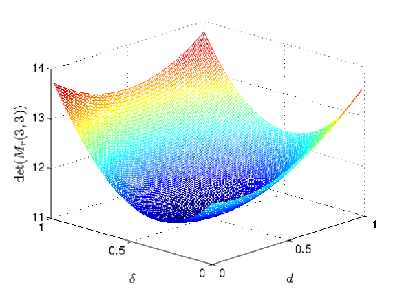
Figure 1: Fisher information on correlation parameters $(\alpha,\beta)$ for $n=m=3$ as function of $d=d_{1}$ and $\delta=\delta_{1}$ in the case $\alpha=0.6,\ \beta=1$.

Now, let us have a look at the free boundary directionally equidistant designs, that is at designs where $d_{1}=d_{2}=\ldots=d_{n-1}=:d$ and $\delta_{1}=\delta_{2}=\ldots=\delta_{m-1}=:\delta$. In this case a D-optimal design is specified by directional distances $d$ and $\delta$ which maximize

$$\det\big{(}M_{r}(n,m)\big{)}=\frac{(n-1)(m-1)d^{2}\delta^{2}}{\big{(}{\mathrm{e}}^{2\alpha d}-1\big{)}^{2}\big{(}{\mathrm{e}}^{2\beta\delta}-1\big{)}^{2}}\Big{(}nm\big{(}{\mathrm{e}}^{2\alpha d}+1\big{)}\big{(}{\mathrm{e}}^{2\beta\delta}+1\big{)}-4(n-1)(m-1)\Big{)}.$$ (2.5)

In the case of OU processes this question does not appear, since for processes Fisher information on covariance parameter based on $n$ equidistant design points depends linearly on the two-point design Fisher information (Kiseľák and Stehlík,, 2008).

Theorem 2.6

If $nm\geq 2(n-1)(m-1)$ then $\det\big{(}M_{r}(n,m)\big{)}$ is strictly monotone decreasing both in $d$ and $\delta$, so its maximum is reached at $d=\delta=0$. If $nm<2(n-1)(m-1)$ then for fixed and small enough $d$ ($\delta$), function $\det\big{(}M_{r}(n,m)\big{)}$ has a single maximum in $\delta$ ($d$).

Remark 2.7

Observe that for $1<n=m\in{\mathbb{N}}$ condition $nm\geq 2(n-1)(m-1)$ is equivalent to $n\leq 3$. Further, if $nm\leq 2(n-1)(m-1)$ then the statement of Theorem 2.6 does not imply the existence of a D-optimal design. Figure 2 shows that the extremal point of $\det\big{(}M_{r}(n,m)\big{)}$ can be a saddle point and the maximum is reached when either $d=0$ or $\delta=0$.

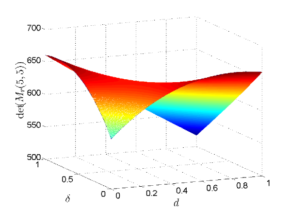
Figure 2: Fisher information of boundary free design on correlation parameters $(\alpha,\beta)$ for $n=m=5$ in the case $\alpha=1,\ \beta=1$.

2.1.3 Estimation of all parameters

Consider now the most general case, when both $\alpha,\ \beta$ and $\theta$ are unknown and the Fisher information matrix on these parameters equals

$$M(n,m)=\begin{bmatrix}M_{\theta}(n,m)&0\\ 0&M_{r}(n,m)\end{bmatrix},$$

where $M_{\theta}(n,m)$ and $M_{r}(n,m)$ are Fisher information matrices on $\theta$ and $r=(\alpha,\beta)^{\top}$, respectively, see (2.2) and (2.3). Thus, the objective function to be maximized is $\det\big{(}M(n,m)\big{)}=M_{\theta}(n,m)\det\big{(}M_{r}(n,m)\big{)}$.

Example 2.8

Consider the nine-point restricted design of Example 2.5, that is $\mathcal{X}=[0,1]^{2}$,  $n=m=3$ and $s_{1}=t_{1}=0,\ s_{2}:=d,\ t_{2}:=\delta,\ s_{3}=t_{3}=1$, implying $d_{1}=d,\ d_{2}=1-d,\ \delta_{1}=\delta,\ \delta_{2}=1-\delta$. In this case from (2.2) and (2.4) we have

$$\det \,\big{(}M(3,3)\big{)}=\bigg{(}1+\frac{{\mathrm{e}}^{\alpha d}-1}{{\mathrm{e}}^{\alpha d}+1}+\frac{{\mathrm{e}}^{\alpha(1-d)}-1}{{\mathrm{e}}^{\alpha(1-d)}+1}\bigg{)}\bigg{(}1+\frac{{\mathrm{e}}^{\beta\delta}-1}{{\mathrm{e}}^{\beta\delta}+1}+\frac{{\mathrm{e}}^{\beta(1-\delta)}-1}{{\mathrm{e}}^{\beta(1-\delta)}+1}\bigg{)}$$

$$\times\Bigg{(}9\bigg{(}\frac{d^{2}\big{(}{\mathrm{e}}^{2\alpha d}+1\big{)}}{\big{(}{\mathrm{e}}^{2\alpha d}-1\big{)}^{2}}+\frac{(1-d)^{2}\big{(}{\mathrm{e}}^{2\alpha(1-d)}+1\big{)}}{\big{(}{\mathrm{e}}^{2\alpha(1-d)}-1\big{)}^{2}}\bigg{)}\bigg{(}\frac{\delta^{2}\big{(}{\mathrm{e}}^{2\beta\delta}+1\big{)}}{\big{(}{\mathrm{e}}^{2\beta\delta}-1\big{)}^{2}}+\frac{(1-\delta)^{2}\big{(}{\mathrm{e}}^{2\beta(1-\delta)}+1\big{)}}{\big{(}{\mathrm{e}}^{2\beta(1-\delta)}-1\big{)}^{2}}\bigg{)}$$ (2.6)

$$-4\bigg{(}\frac{d}{{\mathrm{e}}^{2\alpha d}-1}+\frac{1-d}{{\mathrm{e}}^{2\alpha(1-d)}-1}\bigg{)}^{2}\bigg{(}\frac{\delta}{{\mathrm{e}}^{2\beta\delta}-1}+\frac{1-\delta}{{\mathrm{e}}^{2\beta(1-\delta)}-1}\bigg{)}^{2}\Bigg{)}.$$

Tedious calculations (see Section A.5) show that $\det\big{(}M(3,3)\big{)}$ has a single global minimum at $d=\delta=1/2$, while the maximum is reached at the four vertices of $\mathcal{X}$, namely at $(0,0),\ (0,1),\ (1,0)$ and $(1,1)$. In this way a restricted D-optimal design does not exist.

Again, let us also have a look at the free boundary directionally equidistant designs with directional distances $d$ and $\delta$. The objective function to be maximized in order to get the D-optimal design is

$$\det\big{(}M(n,m)\big{)}= \frac{(n-1)(m-1)d^{2}\delta^{2}}{\big{(}{\mathrm{e}}^{2\alpha d}-1\big{)}^{2}\big{(}{\mathrm{e}}^{2\beta\delta}-1\big{)}^{2}\big{(}{\mathrm{e}}^{\alpha d}+1\big{)}\big{(}{\mathrm{e}}^{\beta\delta}+1\big{)}}\big{(}n({\mathrm{e}}^{\alpha d}-1)+2\big{)}\big{(}m({\mathrm{e}}^{\beta\delta}-1)+2\big{)}$$ (2.7)

$$\times\Big{(}nm\big{(}{\mathrm{e}}^{2\alpha d}+1\big{)}\big{(}{\mathrm{e}}^{2\beta\delta}+1\big{)}-4(n-1)(m-1)\Big{)}.$$

For simplicity assume $n=m$.

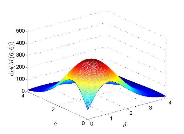
Figure 3: Fisher information of boundary free design on all parameters for $n=m=6$ in the case $\alpha=1,\ \beta=1$.

Theorem 2.9

If $n=2$ then $\det\big{(}M(n,n)\big{)}$ is strictly monotone decreasing both in $d$ and $\delta$, so its maximum is reached at $d=\delta=0$. If $n\geq 3$ then $\det\big{(}M(n,n)\big{)}$ has a global maximum at $(d^{*},\delta^{*})$ which solves

$$n^{2}\big{(}{\mathrm{e}}^{2\beta\delta}+1\big{)}g_{1}(\alpha d,n)=4(n-1)^{2}g_{2}(\alpha d,n),\qquad n^{2}\big{(}{\mathrm{e}}^{2\alpha d}+1\big{)}g_{1}(\beta\delta,n)=4(n-1)^{2}g_{2}(\beta\delta,n),$$ (2.8)

where

$$g_{1}(x,n) :={\mathrm{e}}^{5x}n(1-x)+{\mathrm{e}}^{4x}(2nx-3x-n+2)+{\mathrm{e}}^{3x}x(1-4n)+{\mathrm{e}}^{2x}x(4n-7)+{\mathrm{e}}^{x}(x-n-nx)+n-2,$$

$$g_{2}(x,n) :={\mathrm{e}}^{3x}n(1-2x)+{\mathrm{e}}^{2x}(3nx-5x+2-n)+{\mathrm{e}}^{x}(x-n-nx)+n-2.$$ (2.9)

Theorem 2.9 shows that the situation here completely differs from the case when only covariance parameters are estimated and an optimal free boundary directionally equidistant design does exist. This can clearly be observed on Figure 3 showing $\det\big{(}M(6,6)\big{)}$ for $\alpha=1,\ \beta=1$. Further, simulation results show that for all $n\geq 3$ objective function $\det\big{(}M(n,n)\big{)}$ has a unique maximal point (system (2.8) has a unique solution), however, a rigorous proof of this fact have not been found yet.

2.2 Optimal design with respect to IMSPE criterion

As before, suppose we have observations $\big{\{}Y(s_{i},t_{j}),\ i=1,2,\ldots,n,\ j=1,2,\ldots,m\big{\}}$. The main aim of the kriging technique consists of the prediction of the output of the simulator on the experimental region. For any untried location $(x_{1},x_{2})\in{\mathcal{X}}$ the estimation procedure is focused on the best linear unbiased estimator of $Y(x_{1},x_{2})$ given by $\widehat{Y}(x_{1},x_{2})=\widehat{\theta}+R^{\top}(x_{1},x_{2})C^{-1}(n,m,r)({\mathbf{Y}}-{\mathbf{1}}_{nm}\widehat{\theta})$, where ${\mathbf{Y}}=\big{(}Y(s_{1},t_{1}),Y(s_{1},t_{2}),\ldots,Y(s_{n},t_{m})\big{)}^{\top}$ is the vector of observations, $\widehat{\theta}$ is the generalized least squares estimator of $\theta$, that is $\widehat{\theta}=\big{(}{\mathbf{1}}_{nm}^{\top}C^{-1}(n,m,r){\mathbf{1}}_{nm}\big{)}^{-1}{\mathbf{1}}_{nm}^{\top}C^{-1}(n,m,r){\mathbf{Y}}$, and $R(x_{1},x_{2})$ is the vector of correlations between $Y(x_{1},x_{2})$ and vector ${\mathbf{Y}}$ defined by ​$R(x_{1},x_{2})\!\!=\!\!\big{(}\!\varrho(x_{1},x_{2},s_{1},t_{1}),\ldots,\varrho(x_{1},x_{2},s_{i},t_{j}),\ldots,\varrho(x_{1},x_{2},s_{n},t_{m})\!\big{)}\!^{\top}$​​, where $\varrho(x_{1},x_{2},s_{i},t_{j}):=\varrho_{1}(x_{1},s_{i})\varrho_{2}(x_{2},t_{j})$ with components $\varrho_{1}(x_{1},s_{i}):=\exp\big{(}-\alpha|x_{1}-s_{i}|\big{)}$ and $\varrho_{2}(x_{2},t_{j}):=\exp\big{(}-\beta|x_{2}-t_{j}|\big{)}$. Usually, correlation parameters $\alpha,\beta$ are unknown and will be estimated by maximum likelihood method. Thus, the kriging predictor is obtained by substituting the maximum likelihood estimators (MLE) $(\widehat{\alpha},\widehat{\beta})$ for $(\alpha,\beta)$ and in such a case $\widehat{Y}(x_{1},x_{2})$ is called the MLE-empirical best linear unbiased predictor (Santner et al.,, 2003).

In this way a natural criterion of optimality will minimize suitable functionals of the Mean Squared Prediction Error (MSPE) given by

$$\mathrm{MSPE}\big{(}\widehat{Y}(x_{1},x_{2})\big{)}:=\sigma^{2}\Bigg{[}1-\big{(}1,\,R^{\top}(x_{1},x_{2})\big{)}\left[\BMAT{c.c}{c.c}0&{\mathbf{1}}_{nm}^{\top}\\ {\mathbf{1}}_{nm}C(n,m,r)\right]^{-1}\big{(}1,\,R^{\top}(x_{1},x_{2})\big{)}^{\top}\Bigg{]}.$$ (2.10)

Since the prediction accuracy is often related to the entire prediction region $\mathcal{X}$ the design criterion IMSPE is given by

$$\mathrm{IMSPE}\big{(}\widehat{Y}\big{)}:=\sigma^{-2}\iint\limits_{\mathcal{X}}\mathrm{MSPE}\big{(}\widehat{Y}(x_{1},x_{2})\big{)}\,{\mathrm{d}}x_{1}\,{\mathrm{d}}x_{2}.$$

Theorem 2.10

Let us assume that the design space $\mathcal{X}=[0,1]^{2}$ and since extrapolative prediction is not advisable in kriging, we can set $s_{1}=t_{1}=0$ and $s_{n}=t_{m}=1$.

$$\mathrm{MSPE}\big{(}\widehat{Y}(x_{1},x_{2})\big{)}=\sigma^{2}\Bigg{[}1- \,\bigg{(}\varrho_{1}^{2}(x_{1},s_{n})+\sum_{i=1}^{n-1}\frac{\big{(}\varrho_{1}(x_{1},s_{i})-\varrho_{1}(x_{1},s_{i+1})p_{i}\big{)}^{2}}{1-p_{i}^{2}}\bigg{)}$$

$$\times\bigg{(}\varrho_{2}^{2}(x_{2},t_{m})+\sum_{j=1}^{m-1}\frac{\big{(}\varrho_{2}(x_{2},t_{j})-\varrho_{2}(x_{2},t_{j+1})q_{j}\big{)}^{2}}{1-q_{j}^{2}}\bigg{)}$$ (2.11)

$$+\bigg{(}1+\sum_{i=1}^{n-1}\frac{1-p_{i}}{1+p_{i}}\bigg{)}^{-1} \bigg{(}1+\sum_{j=1}^{m-1}\frac{1-q_{j}}{1+q_{j}}\bigg{)}^{-1}\Bigg{(}1-\bigg{(}\varrho_{1}(x_{1},s_{n})+\sum_{i=1}^{n-1}\frac{\varrho_{1}(x_{1},s_{i})-\varrho_{1}(x_{1},s_{i+1})p_{i}}{1+p_{i}}\bigg{)}$$

$$\times\bigg{(}\varrho_{2}(x_{2},t_{m})+\sum_{j=1}^{m-1}\frac{\varrho_{2}(x_{2},t_{j})-\varrho_{2}(x_{2},t_{j+1})q_{j}}{1+q_{j}}\bigg{)}\Bigg{)}^{2}\Bigg{]},$$

where again $p_{i}:=\exp(-\alpha d_{i}),\ q_{j}:=\exp(-\beta\delta_{j})$ with $d_{i}:=s_{i+1}-s_{i}$ and $\delta_{j}:=t_{j+1}-t_{j},\ i=1,2,\ldots,n-1,\ j=1,2,\ldots,m-1$. Further,

$$\mathrm{IMSPE}\big{(}\widehat{Y}\big{)}= \,1-\bigg{(}\frac{n-1}{\alpha}-2\sum_{i=1}^{n-1}\frac{d_{i}p_{i}^{2}}{1-p_{i}^{2}}\bigg{)}\bigg{(}\frac{m-1}{\beta}-2\sum_{j=1}^{m-1}\frac{\delta_{j}q_{j}^{2}}{1-q_{j}^{2}}\bigg{)}$$ (2.12)

$$+\bigg{(}1+\sum_{i=1}^{n-1}\frac{1-p_{i}}{1+p_{i}}\bigg{)}^{-1}\bigg{(}1+\sum_{j=1}^{m-1}\frac{1-q_{j}}{1+q_{j}}\bigg{)}^{-1}\Bigg{[}1-\frac{8}{\alpha\beta}\bigg{(}\sum_{i=1}^{n-1}\frac{1-p_{i}}{1+p_{i}}\bigg{)}\bigg{(}\sum_{j=1}^{m-1}\frac{1-q_{j}}{1+q_{j}}\bigg{)}$$

$$+\bigg{(}\sum_{i=1}^{n-1}\frac{1-p_{i}^{2}+2\alpha d_{i}p_{i}}{\alpha(1+p_{i})^{2}}\bigg{)}\bigg{(}\sum_{j=1}^{m-1}\frac{1-q_{j}^{2}+2\beta\delta_{j}q_{j}}{\beta(1+q_{j})^{2}}\bigg{)}\Bigg{]}.$$

For any sample size the directionally equidistant design $d_{1}=d_{2}=\ldots=d_{n-1}$ and $\delta_{1}=\delta_{2}=\ldots=\delta_{m-1}$ is optimal with respect to the IMSPE criterion.

Remark 2.11

We remark that (2.12) is an extension of the IMSPE criterion for the classical OU process given by Baldi Antognini and Zagoraiou, (2010, Proposition 4.1), while the optimality result generalizes Proposition 4.2 of Baldi Antognini and Zagoraiou, (2010).

2.3 Optimal design with respect to entropy criterion

Another possible approach to optimal design is to find locations which maximize the amount of obtained information. Following the ideas of Shewry and Wynn, (1987) one has to maximize the entropy $\mathrm{Ent}({\mathbf{Y}})$ of the observations corresponding to the chosen design, which in the Gaussian case form an $nm$-dimensional normal vector with covariance matrix $\sigma^{2}\,C(n,m,r)$, that is

$$\mathrm{Ent}({\mathbf{Y}})=\frac{nm}{2}\big{(}1+\ln(2\pi\sigma^{2})\big{)}+\frac{1}{2}\ln\det C(n,m,r).$$

Theorem 2.12

In our setup entropy $\mathrm{Ent}({\mathbf{Y}})$ has the form

$$\mathrm{Ent}({\mathbf{Y}})=\frac{nm}{2}\big{(}1+\ln(2\pi\sigma^{2})\big{)}+\frac{m}{2}\sum_{i=1}^{n-1}\ln\big{(}1-p_{i}^{2}\big{)}+\frac{n}{2}\sum_{j=1}^{m-1}\ln\big{(}1-q_{j}^{2}\big{)}.$$ (2.13)

For any sample size the directionally equidistant design $d_{1}=d_{2}=\ldots=d_{n-1}$ and $\delta_{1}=\delta_{2}=\ldots=\delta_{m-1}$ is optimal with respect to the entropy criterion.

3 D-optimal designs for the Arrhenius model with OU error

In the present section we derive objective functions for D-optimal designs for estimating parameters of the Arrhenius model (1.1). We consider the stationary process

$$Y(s,t)=\big{(}A/t^{\mu}\big{)}{\mathrm{e}}^{-B/t}+\varepsilon(s,t),$$ (3.1)

observed on a compact design space $\mathcal{X}=[a_{1},b_{1}]\times[a_{2},b_{2}]$, where $b_{1}>a_{1}$ and $b_{2}>a_{2}$ and $\varepsilon(s,t),\ s,t\in{\mathbb{R}}$, is again a stationary Ornstein-Uhlenbeck sheet, that is a zero mean Gaussian process with covariance structure (1.5). Since parameter $A$ is usually known, without loss of generality we may assume $A=1$ and consider model (3.1) with trend function $\eta(s,t;\mu,B):=\big{(}1/t^{\mu}\big{)}{\mathrm{e}}^{-B/t}$.

From the point of view of applications we distinguish two important cases.

• Rate $\mu$ is known, which is an assumption made by several authors, see, e.g., Héberger et al., (1987). The uncorrelated case has already been studied by Rodríguez-Díaz and Santos-Martín, (2009), where the authors proved that for approximated designs a two-point design is optimal.

• Rate $\mu$ is unknown and one has to estimate it together with $B$. For this model the uncorrelated case has also been studied, Rodríguez-Díaz et al., (2012) considered both equidistant and general designs.

3.1 Estimation of trend

Assume that covariance parameters $\alpha,\beta$ and $\sigma$ of the OU sheet and rate $\mu$ of the Arrhenius model are given and we are interested in estimation of the trend parameter $B$. The Fisher information on $B$ based on observations $\big{\{}Y(s_{i},t_{j}),\ i=1,2,\ldots,n,\ j=1,2,\ldots,m\big{\}}$ of the process (3.1) equals $M_{B}(n,m)=F^{\top}(n,m,B)C^{-1}(n,m,r)F^{\top}(n,m,B)$, where

$$F(n,m,B):=\bigg{(}\frac{\eta(s_{1},t_{1};\mu,B)}{\partial B},\frac{\eta(s_{1},t_{2};\mu,B)}{\partial B},\ldots,\frac{\eta(s_{n},t_{m};\mu,B)}{\partial B}\bigg{)}^{\top}.$$

Theorem 3.1

In our setup

$$M_{B}(n,m)=\bigg{(}1+\sum_{i=1}^{n-1}\frac{1-p_{i}}{1+p_{i}}\bigg{)}\bigg{(}\kappa_{m}^{2}+\sum_{j=1}^{m-1}\frac{(\kappa_{j}-\kappa_{j+1}q_{j})^{2}}{1-q_{j}^{2}}\bigg{)},$$ (3.2)

where $\kappa_{j}:=-\exp\big{(}-B/t_{j}\big{)}/t_{j}^{\mu+1}$ if $t_{j}\neq 0$, and $\kappa_{j}:=0$, otherwise.

In case one has to estimate both $\mu$ and $B$, the objective function to be maximized in order to get the D-optimal design is $\det\big{(}M_{\mu,B}(n,m)\big{)}$, where again $M_{\mu,B}(n,m)=G^{\top}(n,m,\mu,B)C^{-1}(n,m,r)G^{\top}(n,m,\mu,B)$ with

$$G(n,m,\mu,B):=\begin{bmatrix}\frac{\eta(s_{1},t_{1};\mu,B)}{\partial\mu}&\frac{\eta(s_{1},t_{2};\mu,B)}{\partial\mu}&\ldots&\frac{\eta(s_{n},t_{m};\mu,B)}{\partial\mu}\\ \frac{\eta(s_{1},t_{1};\mu,B)}{\partial B}&\frac{\eta(s_{1},t_{2};\mu,B)}{\partial B}&\ldots&\frac{\eta(s_{n},t_{m};\mu,B)}{\partial B}\end{bmatrix}^{\top}.$$

Theorem 3.2

In our setup

$$M_{\mu,B}(n,m)= \bigg{(}1+\sum_{i=1}^{n-1}\frac{1-p_{i}}{1+p_{i}}\bigg{)}$$ (3.3)

$$\times\begin{bmatrix}\lambda_{m}^{2}+\sum_{j=1}^{m-1}\frac{(\lambda_{j}-\lambda_{j+1}q_{j})^{2}}{1-q_{j}^{2}}&\lambda_{m}\kappa_{m}+\sum_{j=1}^{m-1}\frac{(\lambda_{j}-\lambda_{j+1}q_{j})(\kappa_{j}-\kappa_{j+1}q_{j})}{1-q_{j}^{2}}\\ \lambda_{m}\kappa_{m}+\sum_{j=1}^{m-1}\frac{(\lambda_{j}-\lambda_{j+1}q_{j})(\kappa_{j}-\kappa_{j+1}q_{j})}{1-q_{j}^{2}}&\kappa_{m}^{2}+\sum_{j=1}^{m-1}\frac{(\kappa_{j}-\kappa_{j+1}q_{j})^{2}}{1-q_{j}^{2}}\end{bmatrix},$$

where $\kappa_{j}$ is the same quantity as in Theorem 3.1, while $\lambda_{j}:=-\log(t_{j})\exp\big{(}-B/t_{j}\big{)}/t_{j}^{\mu}$ if $t_{j}\neq 0$, and $\lambda_{j}:=0$, otherwise.

Theorems 3.1 and 3.2 show that for estimating merely the trend parameters one can treat the two coordinate directions separately. Hence, in the first coordinate direction the maximum is reached with the equidistant design $d_{1}=d_{2}=\ldots=d_{n-1}$, while in the second direction one can consider, e.g., the results of Rodríguez-Díaz et al., (2012) for the classical OU process.

Example 3.3

Consider a four point grid design, i.e. $n=m=2$. Without loss of generality we may assume $s_{1}=t_{1}=0$ implying $s_{2}=d$ and $t_{2}=\delta$. In this case the Fisher information (3.2) on $B$ equals

$$M_{B}(2,2)=\frac{2}{1-\exp(-\alpha d)}\frac{\exp(-2B/\delta)}{\big{(}1-\exp(-2\beta\delta)\big{)}\delta^{2(\mu+1)}},$$

which function is monotone increasing in its first variable $d$. Further, short calculation shows that if $\mu>-1$ then the maximum in $\delta$ is attained at the unique solution of the equation

$$\big{(}B-(\mu+1)\delta\big{)}\big{(}\exp(2\beta\delta)-1\big{)}=\beta\delta^{2}.$$

In case $\mu<-1$, that is in particular interesting for chemometricians, one can employ the maximin approach (see, e.g., Kao et al.,, 2013) which seeks designs maximizing the minimum of the design criterion. In our case this means maximization of

$$\min_{\alpha,\beta>0}M_{B}(2,2)=2\exp(-2B\delta)\delta^{-2(\mu+1)}.$$ (3.4)

Obviously, if $\mu<-1$ then the maximum of (3.4) is reached at $\delta^{*}=-(\mu+1)/B$. Although the maximization of (3.4) is pretty easy, one should take care about the interpretation of such a result as, e.g., the optimal design does not depend on $d$.

Maximin approach, anyhow, cannot be automatized without further considerations since, for instance, maximin designs are of no relevance for criteria, where design distances are multiplied by some nuisance parameters, see, e.g., (2.2).

Remark 3.4

Under the conditions of Example 3.3 ($s_{1}=t_{1}=0$) we have $\det\big{(}M_{\mu,B}(2,2)\big{)}=0$, that is the four point grid design does not provide information on trend parameters $\mu$ and $B$.

3.2 Estimation of all parameters

Assume first that the rate $\mu$ is known and one has to estimate trend parameter $B$ and covariance parameters $(\alpha,\beta)$. Obviously, the Fisher information matrix on these parameters based on observations $\big{\{}Y(s_{i},t_{j}),\ i=1,2,\ldots,n,\ j=1,2,\ldots,m\big{\}}$ of the process (3.1) equals

$${\mathcal{M}}(n,m)=\begin{bmatrix}M_{B}(n,m)&0\\ 0&M_{r}(n,m)\end{bmatrix},$$

where $M_{B}(n,m)$ and $M_{r}(n,m)$ are defined by (3.2) and (2.3), respectively. Hence, in order to obtain a D-optimal design one has to maximize $\det\big{(}{\mathcal{M}}(n,m)\big{)}=M_{B}(n,m)\det\big{(}M_{r}(n,m)\big{)}$.

Example 3.5

Consider again the settings of Example 3.3, that is a four point grid design ($n=m=2$) under the assumption $s_{1}=t_{1}=0$. In this case we have

$${\mathcal{M}}(2,2)=\frac{8d^{2}\exp(-2B/\delta)\exp(-2\beta\delta)\exp(-2\alpha d)\big{(}1+\exp(-2\alpha d)+\exp(-2\beta\delta)\big{)}}{\delta^{2\mu}\big{(}1-\exp(-2\beta\delta)\big{)}^{3}\big{(}1-\exp(-2\alpha d)\big{)}^{2}\big{(}1+\exp(-\alpha d)\big{)}},\qquad d,\delta\geq 0.$$

Tedious calculations (see Section A.11) show that for $d,\delta\geq 0$ function ${\mathcal{M}}(2,2)$ is monotone decreasing in $d$, while in $\delta$ it has a maximum at the unique solution of the equation

$$\beta\delta^{2}-\mu\delta+B+{\mathrm{e}}^{2\beta\delta}\big{(}2\beta(2+p^{2})\delta^{2}+(B-\mu\delta)p^{2}\big{)}+{\mathrm{e}}^{4\beta\delta}(1+p^{2})\big{(}\beta\delta^{2}+\mu\delta-B\big{)}=0.$$

Hence, the optimal four point grid design collapses in its first coordinate.

If rate $\mu$ is also unknown, the Fisher information matrix on $(\mu,B,\alpha,\beta)$ based on $\big{\{}Y(s_{i},t_{j}),\ i=1,2,\ldots,n,\ j=1,2,\ldots,m\big{\}}$ equals

$${\mathfrak{M}}(n,m)=\begin{bmatrix}M_{\mu,B}(n,m)&0\\ 0&M_{r}(n,m)\end{bmatrix},$$

where $M_{\mu,B}(n,m)$ and $M_{r}(n,m)$ are defined by (3.3) and (2.3), respectively. In this case the D-optimal design maximizes objective function $\det\big{(}{\mathfrak{M}}(n,m)\big{)}=\det\big{(}M_{\mu,B}(n,m)\big{)}\det\big{(}M_{r}(n,m)\big{)}$.

4 Comparisons of designs

Methane emissions compose a very complicated process which mixes stochasticity with chaos (see, e.g., Addiscott,, 2010; Sabolová et al.,, 2013), thus fitting of two dimensional OU sheet could be a remedy to several problems which occurred in univariate settings (Rodríguez-Díaz et al.,, 2012). In this section we provide efficiency comparisons for selected important methane kinetic reactions, both in standard (Earth) and non-standard (troposphere) conditions. The current work is the first comprehensive comparison of the statistical information of designs for OU sheets, which gives its novelty both methodologically and from the point of view of applications.

		$\alpha=0.001,\ \beta=0.01$	$\alpha=0.1,\ \beta=1$	$\alpha=1,\ \beta=1$	$\alpha=1,\ \beta=10$
	monotonic	1.3118	29.8651	61.2545	63.9937
$D-opt.$	rectangular	1.3328	57.4388	63.7483	64.00
	rel. eff. (%)	98.43	51.99	96.09	99.99
	monotonic	-33.0446	86.1318	90.7964	90.8121
$entropy$	rectangular	-51.1507	90.7111	90.8119	90.8121
	rel. eff. (%)	64.60	94.95	99.98	100

Table 1: $M_{\theta}(n,m)$ and entropy values corresponding to the optimal monotonic and to the rectangular grid design and relative efficiency of the optimal monotonic design.

4.1 Comparisons of designs for tropospheric methane measurements

As discussed by Lelieveld, (2006), tropospheric methane measurements are fundamental for climate change models and Vaghjiani and Ravishankara, (1991) utilized a $62$ point design to measure the tropospheric methane flux. In Theorem 2.1 the exact form of $M_{\theta}(n,m)$ is derived only for restricted regular designs, however, one might ask what is the relative efficiency of the optimal value of $M_{\theta}(n)$ on monotonic sets (Baran and Stehlík,, 2015) containing $n\times m$ design points compared to the $M_{\theta}(n,m)$ of a rectangular grid with the same number of points. Since the designs for methane used in Vaghjiani and Ravishankara, (1991) typically have around 62 points, we should consider a $64$ point design comparison of, e.g., a $8\times 8$ regular grid with a $64$ points monotonic set for covariance parameters $\alpha,\beta\in\{0.001,0.01,0.1,1,10\}$ and design space $[223,420]\times[0.84,43.51]$.

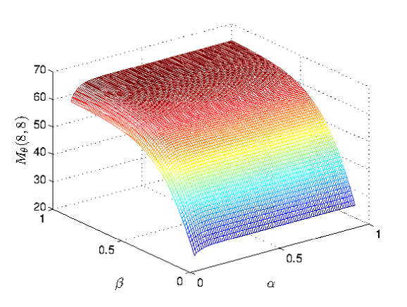
Figure 4: Fisher information on $\theta$ as functions of correlation parameters $(\alpha,\beta)$ for $n=8$ and $m=8$.

Table 1 gives the optimal values of $M_{\theta}(64)$ on monotonic sets, $M_{\theta}(8,8)$ values for regular designs and the relative efficiencies of the optimal $M_{\theta}(64)$ values on monotonic sets for different combinations of parameters $(\alpha,\beta)$. Observe, that for $\alpha=0.1,\,\beta=1$ the optimal monotonic design gives much lower values of Fisher information on $\theta$ than the regular grid, while for the other combinations of parameters the relative efficiency is slightly below $100\,\%$. For the entropy criterion we obtain the same results. In Figure 4 the optimal value of Fisher information on $\theta$ is plotted as a function of correlation parameters $(\alpha,\beta)$ for $n=8$ and $m=8$.

4.2 Comparisons of designs for the rate of methane reactions with $OH$

The growth rate of tropospheric methane is determined by the balance between surface emissions and photo-chemical destruction by the hydroxyl radical $OH,$ the major atmospheric oxidant. Such reaction can happen at various temperature modes, for instance, Bonard et al., (2002) measured the rate constants of the reactions of $OH$ radicals with methane in the temperature range $295-618K$. The following 4 tables provide efficiency of original designs of Bonard et al., (2002) together with efficiencies of monotonic and regular grid designs $3\times 3,\ 2\times 5,\ 5\times 2,\ 3\times 4,\ 4\times 3,\ 3\times 2$ and $2\times 3$, respectively. Tables 2–5 utilize the setups described in Tables 1–4 of Bonard et al., (2002). As one can see, in most of the situations monotonic and regular grid designs outperform the original designs.

		$\alpha\!=\!0.001,\beta\!=\!0.01$	$\alpha\!=\!0.1,\beta\!=\!0.01$	$\alpha\!=\!0.1,\beta\!=\!1$	$\alpha\!=\!1,\beta\!=\!1$	$\alpha\!=\!1,\beta\!=\!10$
	Bonard et al., (2002)	3.1261	8.7785	8.9904	9.0000	9.0000
$D-opt.$	mon., $n=9$	3.2067	8.9107	9.0000	9.0000	9.0000
	$3\times 3$ r.grid	3.0305	7.6660	9.0000	9.0000	9.0000
	Bonard et al., (2002)	9.8567	12.7665	12.7704	12.7704	12.7704
$Ent.$	mon., $n=9$	11.2150	12.7703	12.7704	12.7704	12.7704
	$3\times 3$ r.grid	9.2225	12.7231	12.7704	12.7704	12.7704

Table 2: $M_{\theta}(n,m)$ and entropy values corresponding to the optimal monotonic and to the rectangular grid design together with values of optimality criteria for measurements given in Bonard et al., (2002, Table 1).

		$\alpha\!=\!0.001,\beta\!=\!0.01$	$\alpha\!=\!0.1,\beta\!=\!0.01$	$\alpha\!=\!0.1,\beta\!=\!1$	$\alpha\!=\!1,\beta\!=\!1$	$\alpha\!=\!1,\beta\!=\!10$
	Bonard et al., (2002)	1.1853	6.9087	7.0855	8.7813	9.2477
$D-opt.$	mon., $n=10$	1.1858	9.5186	9.7151	10.0000	10.0000
	$2\times 5$ r.grid	1.1884	2.0487	6.3460	6.3460	9.9999
	$5\times 2$ r.grid	1.1897	5.1192	9.9189	9.9239	10.0000
	Bonard et al., (2002)	-0.8169	11.9268	12.5103	14.0660	14.1336
$Ent.$	mon., $n=10$	2.7830	14.1860	14.1882	14.1894	14.1894
	$2\times 5$ r.grid	-2.5767	-0.7201	13.8227	13.8227	14.1894
	$5\times 2$ r.grid	0.6346	8.2463	14.1892	14.1892	14.1894

Table 3: $M_{\theta}(n,m)$ and entropy values corresponding to the optimal monotonic and to the rectangular grid design together with values of optimality criteria for measurements given in Bonard et al., (2002, Table 2).

		$\alpha\!=\!0.001,\beta\!=\!0.01$	$\alpha\!=\!0.1,\beta\!=\!0.01$	$\alpha\!=\!0.1,\beta\!=\!1$	$\alpha\!=\!1,\beta\!=\!1$	$\alpha\!=\!1,\beta\!=\!10$
	Bonard et al., (2002)	1.1816	6.7348	6.9218	7.6265	9.0242
$D-opt.$	mon., $n=12$	1.1818	10.8570	11.2215	12.0000	12.0000
	$3\times 4$ r.grid	1.1850	3.0669	8.6804	8.6804	12.0000
	$4\times 3$ r.grid	1.1852	4.0890	10.4462	10.4466	12.0000
	Bonard et al., (2002)	-5.7821	3.0845	12.3312	12.9532	16.4642
$Ent.$	mon., $n=12$	1.9060	17.0107	17.0199	17.0273	17.0273
	$3\times 4$ r.grid	-4.0505	1.1408	16.7911	16.7911	17.0273
	$4\times 3$ r.grid	-2.9378	4.4983	16.9807	16.9807	17.0273

Table 4: $M_{\theta}(n,m)$ and entropy values corresponding to the optimal monotonic and to the rectangular grid design together with values of optimality criteria for measurements given in Bonard et al., (2002, Table 3).

		$\alpha\!=\!0.001,\beta\!=\!0.01$	$\alpha\!=\!0.1,\beta\!=\!0.01$	$\alpha\!=\!0.1,\beta\!=\!1$	$\alpha\!=\!1,\beta\!=\!1$	$\alpha\!=\!1,\beta\!=\!10$
	Bonard et al., (2002), $n=7$	1.0057	1.1531	1.5630	2.2240	4.5042
	Bonard et al., (2002), $n=6$	1.0057	1.1531	1.5630	2.2240	4.4850
$D-opt.$	mon.,$n=7$	1.0057	1.1542	1.5683	2.8570	5.4387
	mon.,$n=6$	1.0057	1.1542	1.5675	2.8309	5.0721
	$2\times 3$ r.grid	1.0057	1.1537	1.6244	2.6938	5.6029
	$3\times 2$ r.grid	1.0057	1.1545	1.6061	3.1714	4.5396
	Bonard et al., (2002), $n=7$	-8.3075	-6.4357	4.9754	5.1821	8.9398
	Bonard et al., (2002), $n=6$	-5.4333	-3.5616	5.5473	5.7539	8.3806
$Ent.$	mon., $n=7$	-6.7914	2.9548	6.4778	8.9552	9.8647
	mon., $n=6$	-4.9681	3.1294	6.0021	7.9077	8.4873
	$2\times 3$ r.grid	-8.7323	-2.2476	6.1896	7.3797	8.5095
	$3\times 2$ r.grid	-9.2498	-0.3290	5.5038	8.1021	8.4115

Table 5: $M_{\theta}(n,m)$ and entropy values corresponding to the optimal monotonic and to the rectangular grid design together with values of optimality criteria for measurements given in Bonard et al., (2002, Table 4).

Dunlop and Tully, (1993) measured absolute rate coefficients for the reactions of $OH$ radical with $CH_{4}$ ($k_{1}$) and perdeuterated methane $d_{4}$ ($k_{2}$.) Authors characterized $k_{1}$ and $k_{2}$ over the temperature range $293-800K.$ Finally, they found an excellent agreement of their results with determinations of $k_{1}$ at lower temperatures of Vaghjiani and Ravishankara, (1991). Now, let us consider rates $k_{1}$ and $k_{2}$ of Table 1 of Dunlop and Tully, (1993). We obtain the following comparisons (Table 6-7) of efficiencies of the monotonic and $2\times 5$ and $5\times 2$ regular grid designs with the original designs of Dunlop and Tully, (1993). These results show that in most of the cases, the monotonic and regular grid designs are more efficient than the original one.

		$\alpha\!=\!0.001,\beta\!=\!0.01$	$\alpha\!=\!0.1,\beta\!=\!0.01$	$\alpha\!=\!0.1,\beta\!=\!1$	$\alpha\!=\!1,\beta\!=\!1$	$\alpha\!=\!1,\beta\!=\!10$
	Dunlop and Tully, (1993)	4.5728	9.4857	9.9959	10.0000	10.0000
$D-opt.$	mon., $n=10$	4.7604	9.9721	10.0000	10.0000	10.0000
	$2\times 5$ r.grid	4.9144	7.8743	10.0000	10.0000	10.0000
	$5\times 2$ r.grid	2.5049	9.9944	9.9999	10.0000	10.0000
	Dunlop and Tully, (1993)	12.2328	14.1366	14.1894	14.1894	14.1894
$Ent.$	mon., $n=10$	13.3584	14.1894	14.1894	14.1894	14.1894
	$2\times 5$ r.grid	12.9678	14.0944	14.1894	14.1894	14.1894
	$5\times 2$ r.grid	8.2035	14.1894	14.1894	14.1894	14.1894

Table 6: $M_{\theta}(n,m)$ and entropy values corresponding to the optimal monotonic and to the rectangular grid design together with values of optimality criteria for $k_{1}$ measurements given in Dunlop and Tully, (1993, Table 1).

		$\alpha\!=\!0.001,\beta\!=\!0.01$	$\alpha\!=\!0.1,\beta\!=\!0.01$	$\alpha\!=\!0.1,\beta\!=\!1$	$\alpha\!=\!1,\beta\!=\!1$	$\alpha\!=\!1,\beta\!=\!10$
	Dunlop and Tully, (1993)	3.0778	11.7720	11.9798	12.0000	12.0000
$D-opt.$	mon., $n=12$	3.1465	11.8465	12.0000	12.0000	12.0000
	$3\times 4$ r.grid	3.3749	8.0858	12.0000	12.0000	12.0000
	$4\times 3$ r.grid	3.1184	9.9557	12.0000	12.0000	12.0000
	Dunlop and Tully, (1993)	11.2608	17.0260	17.0272	17.0273	17.0273
$Ent.$	mon., $n=12$	13.7036	17.0270	17.0273	17.0273	17.0273
	$3\times 4$ r.grid	12.9774	16.6656	17.0273	17.0273	17.0273
	$4\times 3$ r.grid	11.3202	16.9405	17.0273	17.0273	17.0273

Table 7: $M_{\theta}(n,m)$ and entropy values corresponding to the optimal monotonic and to the rectangular grid design together with values of optimality criterion for $k_{2}$ measurements given in Dunlop and Tully, (1993, Table 2).

5 Conclusions

Both Kyoto protocol (Lelieveld,, 2006) and recent Scandinavian and Polish summits in 2013 pointed out necessity to develop precise statistical modelling of climate change. This, in particular should be addressed by developing of optimal, or at least benchmarking designs for complex climatic models. The current work aims to contribute here for the case of methane modelling in troposphere, lowest part of atmosphere. As can be well seen in the paper, optimal designs for univariate case (OU process, see Rodríguez-Díaz et al., (2012)) and planar OU sheets differ. Obviously, planar OU sheet is much more precise, since it allows variability both in temperature (main chemically understood driver of chemical kinetics) and in a second variable, which can be either atmospheric pressure or any other relevant quantity. Temperature itself is also regressor, i.e. variable entering into trend parameter $k_{1}$. One valuable further research direction, enabled by the second variable “$s$” will be direct modelling of reaction kinetics. The optimal design for spatial process of methane flux can be helpful for better understanding the emerging issues of paleoclimatology (McShane and Wyner, 2011), ), which in major part relates to large variability.

Acknowledgment. This research has been supported by the Hungarian –Austrian intergovernmental S&T cooperation program TÉT_10-1-2011-0712 and partially supported the TÁMOP-4.2.2.C-11/1/KONV-2012-0001 project. The project has been supported by the European Union, co-financed by the European Social Fund. M. Stehlík acknowledges the support of ANR project Desire FWF I 833-N18 and Fondecyt Proyecto Regular N° 1151441. K. Sikolya has been supported by TÁMOP 4.2.4. A/2-11-1-2012-0001 project “National Excellence Program – Elaborating and operating an inland student and researcher personal support system”. The project was subsidized by the European Union and co-financed by the European Social Fund.

Appendix A Appendix

A.1 Proof of Theorem 2.1

According to the notations of Section 2.1 let $d_{i}:=s_{i+1}-s_{i},\ \delta_{j}:=t_{j+1}-t_{j}$ and $p_{i}:=\exp(-\alpha d_{i}),$
$\ q_{j}:=\exp(-\beta\delta_{j})$. Short calculation shows that

$$C(n,m,r)=P(n,r)\otimes Q(m,r),$$ (A.1)

where

$$P(n,r):= \,\begin{bmatrix}1&p_{1}&p_{1}p_{2}&p_{1}p_{2}p_{3}&\dots&\dots&\prod_{i=1}^{n-1}p_{i}\\ p_{1}&1&p_{2}&p_{2}p_{3}&\dots&\dots&\prod_{n=2}^{n-1}p_{i}\\ p_{1}p_{2}&p_{2}&1&p_{3}&\dots&\dots&\prod_{i=3}^{n-1}p_{i}\\ p_{1}p_{2}p_{3}&p_{2}p_{3}&p_{3}&1&\dots&\dots&\vdots\\ \vdots&\vdots&\vdots&\vdots&\ddots&&\vdots\\ \vdots&\vdots&\vdots&\vdots&&\ddots&p_{n-1}\\ \prod_{i=1}^{n-1}p_{i}&\prod_{i=2}^{n-1}p_{i}&\prod_{i=3}^{n-1}p_{i}&\dots&\dots&p_{n-1}&1\\ \end{bmatrix},$$

$$Q(m,r):= \,\begin{bmatrix}1&q_{1}&q_{1}q_{2}&q_{1}q_{2}q_{3}&\dots&\dots&\prod_{j=1}^{m-1}q_{j}\\ q_{1}&1&q_{2}&q_{2}q_{3}&\dots&\dots&\prod_{j=2}^{m-1}q_{j}\\ q_{1}q_{2}&q_{2}&1&q_{3}&\dots&\dots&\prod_{j=3}^{m-1}q_{j}\\ q_{1}q_{2}q_{3}&q_{2}q_{3}&q_{3}&1&\dots&\dots&\vdots\\ \vdots&\vdots&\vdots&\vdots&\ddots&&\vdots\\ \vdots&\vdots&\vdots&\vdots&&\ddots&q_{m-1}\\ \prod_{j=1}^{m-1}q_{j}&\prod_{j=2}^{m-1}q_{j}&\prod_{j=3}^{m-1}q_{j}&\dots&\dots&q_{m-1}&1\\ \end{bmatrix}.$$

By the properties of the Kronecker product

$$C^{-1}(n,m,r)=P^{-1}(n,r)\otimes Q^{-1}(m,r),$$ (A.2)

and, according to the results of Kiseľák and Stehlík, (2008), e.g., the inverse of $P(n,r)$ equals

$$P^{-1}(n,r)=\begin{bmatrix}\frac{1}{1-p_{1}^{2}}&\frac{p_{1}}{p_{1}^{2}-1}&0&0&\dots&\dots&0\\ \frac{p_{1}}{p_{1}^{2}-1}&V_{2}&\frac{p_{2}}{p_{2}^{2}-1}&0&\dots&\dots&0\\ 0&\frac{p_{2}}{p_{2}^{2}-1}&V_{3}&\frac{p_{3}}{p_{3}^{2}-1}&\dots&\dots&0\\ 0&0&\frac{p_{3}}{p_{3}^{2}-1}&V_{4}&\dots&\dots&\vdots\\ \vdots&\vdots&\vdots&\vdots&\ddots&&\vdots\\ \vdots&\vdots&\vdots&\vdots&&V_{n-1}&\frac{p_{n-1}}{p_{n-1}^{2}-1}\\ 0&0&0&\dots&\dots&\frac{p_{n-1}}{p_{n-1}^{2}-1}&\frac{1}{1-p_{n-1}^{2}}\\ \end{bmatrix},$$ (A.3)

where $V_{k}:=\frac{1-p_{k}^{2}p_{k-1}^{2}}{(p_{k}^{2}-1)(p_{k-1}^{2}-1)}=\frac{1}{1-p_{k}^{2}}+\frac{p_{k-1}^{2}}{1-p_{k-1}^{2}},\ k=2,\dots,n-1$. Obviously, ${\mathbf{1}}_{nm}={\mathbf{1}}_{n}\otimes{\mathbf{1}}_{m}$, and in this way

$$M_{\theta}(n,m)={\mathbf{1}}_{nm}^{\top}C^{-1}(n,m,r){\mathbf{1}}_{nm}= \big{(}{\mathbf{1}}_{n}^{\top}\otimes{\mathbf{1}}_{m}^{\top}\big{)}\big{(}P^{-1}(n,r)\otimes Q^{-1}(m,r)\big{)}\big{(}{\mathbf{1}}_{n}\otimes{\mathbf{1}}_{m}\big{)}$$

$$= \big{(}{\mathbf{1}}_{n}^{\top}P^{-1}(n,r){\mathbf{1}}_{n}\big{)}\big{(}{\mathbf{1}}_{m}^{\top}Q^{-1}(m,r){\mathbf{1}}_{m}\big{)}.$$

Further, by the same arguments as in Baran and Stehlík, (2015) we have

$${\mathbf{1}}_{n}^{\top}P^{-1}(n,r){\mathbf{1}}_{n}=1+\sum_{i=1}^{n-1}\frac{1-p_{i}}{1+p_{i}}\qquad\text{and}\qquad{\mathbf{1}}_{m}^{\top}Q^{-1}(m,r){\mathbf{1}}_{m}=1+\sum_{j=1}^{m-1}\frac{1-q_{j}}{1+q_{j}},$$ (A.4)

implying

$$M_{\theta}(n,m)\!=\!M_{\theta}^{(1)}(n)M_{\theta}^{(2)}(m),\quad\text{where}\quad M_{\theta}^{(1)}(n)\!:=\!1\!+\!\sum_{i=1}^{n-1}\frac{1\!-\!p_{i}}{1\!+\!p_{i}},\ \ M_{\theta}^{(2)}(m)\!:=\!1\!+\!\sum_{j=1}^{m-1}\frac{1\!-\!q_{j}}{1\!+\!q_{j}}.$$

Now, consider reformulation

$$M_{\theta}^{(1)}(n)=1+\sum_{i=1}^{n-1}g\big{(}\alpha d_{i}\big{)},\qquad M_{\theta}^{(2)}(n)=1+\sum_{j=1}^{m-1}g\big{(}\beta\delta_{j}\big{)}\qquad\text{where}\quad g(x):=\frac{1-\exp(-x)}{1+\exp(-x)}.$$

As $g(x)$ is a concave function of $x$, by Marshall and Olkin, (1979, Proposition C1, p. 64), $M_{\theta}^{(1)}(n)$ and $M_{\theta}^{(2)}(m)$ are Schur-concave functions of their arguments $d_{i},\ i=1,2,\ldots,n-1$, and $\delta_{j},\ j=1,2,\ldots,m-1$, respectively. In this way $M_{\theta}(n,m)$ attains its maximum at $d_{1}=d_{2}=\ldots=d_{n-1}$ and $\delta_{1}=\delta_{2}=\ldots=\delta_{m-1}$, which completes the proof. $\square$

A.2 Proof of Theorem 2.2

By representation (A.1) and the properties of the Kronecker product we have

$$M_{\alpha}(n,m) =\frac{1}{2}\mathrm{tr}\left\{\Bigg{(}\Big{(}P^{-1}(n,r)\otimes Q^{-1}(m,r)\Big{)}\bigg{(}\frac{\partial P(n,r)}{\partial\alpha}\otimes Q(m,r)\bigg{)}\Bigg{)}^{2}\right\}$$

$$=\frac{1}{2}\mathrm{tr}\left\{\bigg{(}P^{-1}(n,r)\frac{\partial P(n,r)}{\partial\alpha}\bigg{)}^{2}\otimes{\mathcal{I}}_{m}\right\}=\frac{m}{2}\mathrm{tr}\left\{\bigg{(}P^{-1}(n,r)\frac{\partial P(n,r)}{\partial\alpha}\bigg{)}^{2}\right\},$$

where ${\mathcal{I}}_{m}$ denotes the $m\times m$ unit matrix. Now, the same ideas that lead to the proof of Baran and Stehlík, (2015, Theorem 2) (see also Baldi Antognini and Zagoraiou,, 2010, Proposition 6.1) imply the first equation of (2.4). The form of $M_{\beta}(n,m)$ follows by symmetry. Finally,

$$M_{\alpha,\beta}(n,m)= \frac{1}{2}\mathrm{tr}\Bigg{\{}\big{(}P^{-1}(n,r)\otimes Q^{-1}(m,r)\big{)}\bigg{(}\frac{\partial P(n,r)}{\partial\alpha}\otimes Q(m,r)\bigg{)}$$

$$\phantom{\frac{1}{2}\mathrm{tr}\Bigg{\{}}\times\big{(}P^{-1}(n,r)\otimes Q^{-1}(m,r)\big{)}\bigg{(}P(n,r)\otimes\frac{\partial Q(m,r)}{\partial\beta}\bigg{)}\Bigg{\}}$$

$$= \frac{1}{2}\mathrm{tr}\left\{\Bigg{(}\bigg{(}P^{-1}(n,r)\frac{\partial P(n,r)}{\partial\alpha}\bigg{)}\otimes{\mathcal{I}}_{m}\Bigg{)}\Bigg{(}{\mathcal{I}}_{n}\otimes\bigg{(}Q^{-1}(m,r)\frac{\partial Q(m,r)}{\partial\beta}\bigg{)}\Bigg{)}\right\}$$

$$= \frac{1}{2}\mathrm{tr}\left\{P^{-1}(n,r)\frac{\partial P(n,r)}{\partial\alpha}\right\}\mathrm{tr}\left\{Q^{-1}(m,r)\frac{\partial Q(m,r)}{\partial\beta}\right\},$$

so the last statement of Theorem 2.2 follows from Zagoraiou and Baldi Antognini, (2009, Theorem 3.1) (see also Baldi Antognini and Zagoraiou, (2010, Proposition 6.1)). $\square$

A.3 Proof of Theorem 2.4

Consider first the case when we are interested in estimation of one of the parameters $\alpha$ and $\beta$ and other parameters are considered as nuisance. According to Remark 2.3, in this situation the statement of the theorem directly follows from the corresponding result for OU processes, see Zagoraiou and Baldi Antognini, (2009, Theorem 4.2)

Now, consider the case when both $\alpha$ and $\beta$ are unknown. According to (2.3) and (2.4) the corresponding objective function to be maximized is

$$\Phi(d_{1}, \,\ldots,d_{n-1},\delta_{1},\ldots,\delta_{m-1})=\det\big{(}M_{r}(n,m)\big{)}$$ (A.5)

$$=nm\Bigg{(}\sum_{i=1}^{n-1}\frac{d_{i}^{2}p_{i}^{2}(1+p_{i}^{2})}{(1-p_{i}^{2})^{2}}\Bigg{)}\Bigg{(}\sum_{j=1}^{m-1}\frac{\delta_{j}^{2}q_{j}^{2}(1+q_{j}^{2})}{(1-q_{j}^{2})^{2}}\Bigg{)}-4\Bigg{(}\sum_{i=1}^{n-1}\frac{d_{i}p_{i}^{2}}{1-p_{i}^{2}}\Bigg{)}^{2}\Bigg{(}\sum_{j=1}^{m-1}\frac{\delta_{j}q_{j}^{2}}{1-q_{j}^{2}}\Bigg{)}^{2},$$

which is non-negative, due to Cauchy-Schwartz inequality. Short calculation shows

$$\Phi(d_{1},\ldots,d_{n-1},\delta_{1},\ldots,\delta_{m-1})= \,\bigg{(}n\sum_{i=1}^{n-1}g(d_{i},\alpha)\bigg{)}\left(m\sum_{j=1}^{m-1}g(\delta_{j},\beta)-2\bigg{(}\sum_{j=1}^{m-1}h(\delta_{j},\beta)\bigg{)}^{2}\right)$$ (A.6)

$$+2\bigg{(}\sum_{j=1}^{m-1}h(\delta_{j},\beta)\bigg{)}^{2}\left(n\sum_{i=1}^{n-1}g(d_{i},\alpha)-2\bigg{(}\sum_{i=1}^{n-1}h(d_{i},\alpha)\bigg{)}^{2}\right),$$

where

$$g(x,\gamma):=\frac{x^{2}\big{(}\exp(2\gamma x)+1\big{)}}{\big{(}\exp(2\gamma x)-1\big{)}^{2}}\qquad\text{and}\qquad h(x,\gamma):=\frac{x}{\exp(2\gamma x)-1}.$$ (A.7)

In this way one can consider the two coordinate directions separately.

Since for a given parameter value $\gamma$ both $g(x,\gamma)$ (Zagoraiou and Baldi Antognini,, 2009, Theorem 4.2) and $h(x,\gamma)$ (Baldi Antognini and Zagoraiou,, 2010, Theorem 4.2) are convex functions of $x$, according to Marshall and Olkin, (1979, Proposition C1, p. 64)

$$\sum_{i=1}^{n-1}g(d_{i},\alpha)\qquad\text{and}\qquad\bigg{(}\sum_{j=1}^{m-1}h(\delta_{j},\beta)\bigg{)}^{2}$$

are Schur-convex functions on $[0,1]^{n-1}$ and $[0,1]^{m-1}$, respectively. In this way, they can attain their maxima on the frontiers of their domains of definition.

Finally, consider the constrained optimum of, e.g.,

$$\Psi(d_{1},\ldots,d_{n-1}):=n\sum_{i=1}^{n-1}g(d_{i},\alpha)-2\bigg{(}\sum_{i=1}^{n-1}h(d_{i},\alpha)\bigg{)}^{2},\qquad\text{given}\qquad\sum_{i=1}^{n-1}d_{i}=1.$$

Equating the partial derivatives of the Lagrange function

$$\Lambda(d_{1},\ldots d_{n-1};\lambda):=\Psi(d_{1},\ldots,d_{n-1})+\lambda(d_{1}+\ldots+d_{n-1}-1)$$

to zero results in equations

$$ng^{\prime}(d_{k},\alpha)-4\bigg{(}\sum_{i=1}^{n-1}h(d_{i},\alpha)\bigg{)}h^{\prime}(d_{k},\alpha)+\lambda=0,\qquad k=1,2,\ldots,n-1.$$

This means that the optimum point of $\Psi$ in $[0,1]^{n-1}$ corresponds to the equidistant design $d_{1}=d_{2}=\ldots$ $=d_{n-1}=1/(n-1)$. $\square$

A.4 Proof of Theorem 2.6

Observe first that instead of $\det\big{(}M_{r}(n,m)\big{)}$ given by (2.5) it suffices to investigate the behaviour of the function

$$G(x,y):=\frac{x^{2}y^{2}}{({\mathrm{e}}^{x}-1)^{2}({\mathrm{e}}^{y}-1)^{2}}\Big{(}nm({\mathrm{e}}^{x}+1)({\mathrm{e}}^{y}+1)-4(n-1)(m-1)\Big{)},\qquad x,y\geq 0.$$

Obviously,

$$\frac{\partial G(x,y)}{\partial x}=\frac{xy^{2}}{({\mathrm{e}}^{x}-1)^{3}({\mathrm{e}}^{y}-1)^{2}}\Big{(}nm({\mathrm{e}}^{y}+1)\big{(}(2-x){\mathrm{e}}^{2x}-3x{\mathrm{e}}^{x}-2\big{)}+8(n-1)(m-1)\big{(}1-(1-x){\mathrm{e}}^{x}\big{)}\Big{)},$$

which equals $0$ for non-zero values of $x$ and $y$ if and only if

$$\frac{1-(1-x){\mathrm{e}}^{x}}{(x-2){\mathrm{e}}^{2x}+3x{\mathrm{e}}^{x}+2}=\frac{nm({\mathrm{e}}^{y}+1)}{8(n-1)(m-1)}.$$ (A.8)

Now, the left-hand side of (A.8) is strictly monotone decreasing and has a range of $[0,1/2]$. If $nm\geq 2(n-1)(m-1)$ then for $y>0$ the right-hand side of (A.8) is greater than $1/2$, so in this case $\frac{\partial G(x,y)}{\partial x}<0$. Finally, if $nm<2(n-1)(m-1)$ and $y$ is fixed and small enough then the right-hand side of (A.8) is less than $1/2$, so $\frac{\partial G(x,y)}{\partial x}=0$ in a single point $x$, where $G(x,y)$ takes its maximum. $\square$

A.5 Calculations for Example 2.8

Decomposition (A.6) of $\det\big{(}M_{r}(3,3)\big{)}$ implies

$$\det\big{(}M(3,3)\big{)}= \,\Big{[}3\big{(}1+\phi(d,\alpha)+\phi(1-d,\alpha)\big{)}\big{(}g(d,\alpha)+g(1-d,\alpha)\big{)}\Big{]}$$

$$\times\bigg{[}\big{(}1+\phi(\delta,\beta)+\phi(1-\delta,\beta)\big{)}\Big{(}3\big{(}g(\delta,\beta)+g(1-\delta,\beta)\big{)}-2\big{(}h(\delta,\beta)+h(1-\delta,\beta)\big{)}^{2}\Big{)}\bigg{]}$$ (A.9)

$$+\bigg{[}\big{(}1+\phi(d,\alpha)+\phi(1-d,\alpha)\big{)}\Big{(}3\big{(}g(d,\alpha)+g(1-d,\alpha)\big{)}-2\big{(}h(d,\alpha)+h(1-d,\alpha)\big{)}^{2}\Big{)}\bigg{]}$$

$$\times\Big{[}2\big{(}1+\phi(\delta,\beta)+\phi(1-\delta,\beta)\big{)}\big{(}h(\delta,\beta)+h(1-\delta,\beta)\big{)}^{2}\Big{]},$$

where $g(x,\gamma)$ and $h(x,\gamma)$ are defined by (A.7) and

$$\phi(x,\gamma):=\frac{\exp(\gamma x)-1}{\exp(\gamma x)+1}.$$

In this way one can separate $d$ and $\delta$ and it suffices to investigate the behaviour of functions

$$\Phi_{1}(x,\gamma):= \,\Psi_{1}(x,\gamma)\Psi_{2}(x,\gamma),\qquad\Phi_{2}(x,\gamma):=\Psi_{1}(x,\gamma)\big{(}\Psi_{2}(x,\gamma)\big{)}^{2},$$

$$\Phi_{3}(x,\gamma):=\Psi_{1}(x,\gamma)\Big{(}3\Psi_{2}(x,\gamma)-2\big{(}\Psi_{3}(x,\gamma)\big{)}^{2}\Big{)},$$

where $x\in[0,1],\ \gamma>0$ and

$$\Psi_{1}(x,\gamma) :=1+\phi(x,\gamma)+\phi(1\!-\!x,\gamma),\quad\Psi_{2}(x,\gamma):=g(x,\gamma)+g(1\!-\!x,\gamma),\quad\Psi_{3}(x,\gamma):=h(x,\gamma)+h(1\!-\!x,\gamma).$$

$\Psi_{1}(x,\gamma),\ \Psi_{2}(x,\gamma)$ and $\Psi_{3}(x,\gamma)$ are symmetric in $x$ on $1/2$ and obviously, the same property holds for $\Phi_{1}(x,\gamma),\ \Phi_{2}(x,\gamma)$ and $\Phi_{3}(x,\gamma)$. Further, as $\frac{\partial\phi(x,\gamma)}{\partial x}$ is strictly monotone decreasing, while $\frac{\partial g(x,\gamma)}{\partial x}$ and $\frac{\partial h(x,\gamma)}{\partial x}$ are strictly monotone increasing, $\Psi_{1}$ is strictly concave, while $\Psi_{2}$ and $\Psi_{3}$ are strictly convex functions of $x$.

Consider first $\Phi_{1}(x,\gamma)$. As

$$\Psi_{1}(0,\gamma)\leq\Psi_{1}(x,\gamma)\leq\Psi_{1}(1/2,\gamma)\quad\text{and}\quad\Psi_{2}(1/2,\gamma)\leq\Psi_{2}(x,\gamma)\leq\Psi_{2}(0,\gamma),\qquad x\in[0,1],$$

we have

$$\frac{\partial\Phi_{1}(x,\gamma)}{\partial x}\begin{cases}\leq{\mathcal{Y}}(x,\gamma),&\text{if $0<x<1/2$;}\\ \geq{\mathcal{Y}}(x,\gamma),&\text{if $1/2\leq x<1$,}\end{cases}$$ (A.10)

where

$${\mathcal{Y}}(x,\gamma):=\frac{\partial\Psi_{1}(x,\gamma)}{\partial x}\Psi_{2}(0,\gamma)+\frac{\partial\Psi_{2}(x,\gamma)}{\partial x}\Psi_{1}(0,\gamma)=\Upsilon(x,\gamma)-\Upsilon(1-x,\gamma),$$ (A.11)

with

$$\Upsilon(x,\gamma):=\frac{\partial\phi(x,\gamma)}{\partial x}\frac{{\mathrm{e}}^{2\gamma}\!+\!1}{({\mathrm{e}}^{2\gamma}\!-\!1)^{2}}+\frac{\partial g(x,\gamma)}{\partial x}\frac{2{\mathrm{e}}^{\gamma}}{{\mathrm{e}}^{\gamma}\!+\!1}=\frac{2\gamma{\mathrm{e}}^{\gamma x}({\mathrm{e}}^{2\gamma}\!+\!1)}{({\mathrm{e}}^{\gamma x}\!+\!1)^{2}({\mathrm{e}}^{2\gamma}\!-\!1)^{2}}-\frac{4x{\mathrm{e}}^{\gamma}(3\gamma x{\mathrm{e}}^{2\gamma x}\!-\!{\mathrm{e}}^{4\gamma x}\!+\!\gamma x{\mathrm{e}}^{4\gamma x}\!+\!1)}{({\mathrm{e}}^{2\gamma x}\!-\!1)^{3}({\mathrm{e}}^{\gamma}\!+\!1)}.$$

Further, let

$$\frac{\partial\Upsilon(x,\gamma)}{\partial x}=\frac{\Upsilon^{(1)}(x,\gamma)}{\Upsilon^{(2)}(x,\gamma)},$$

where for $x>0$ the denominator $\Upsilon^{(2)}(x,\gamma)=({\mathrm{e}}^{2\gamma x}-1)^{4}({\mathrm{e}}^{2\gamma}-1)^{2}$ is obviously positive, while the numerator can be written as

$$\Upsilon^{(1)}(x,\gamma)= \,4{\mathrm{e}}^{\gamma}({\mathrm{e}}^{2\gamma}\!-\!1)({\mathrm{e}}^{\gamma}\!-\!1)\Big{(}{\mathrm{e}}^{6\gamma x}\big{(}2\gamma^{2}x^{2}\!-\!4\gamma x\!+\!1\big{)}\!+\!{\mathrm{e}}^{4\gamma x}\big{(}16\gamma^{2}x^{2}\!-\!8\gamma x\!-\!1\big{)}\!+\!{\mathrm{e}}^{2\gamma x}\big{(}6\gamma^{2}x^{2}\!+\!12\gamma x\!-\!1\big{)}\!+\!1\Big{)}$$

$$-2\gamma^{2}({\mathrm{e}}^{2\gamma}\!+\!1){\mathrm{e}}^{\gamma x}({\mathrm{e}}^{\gamma x}\!-\!1)^{5}({\mathrm{e}}^{\gamma x}\!+\!1).$$

If $x\in[0,1]$ then by inequality

$$2{\mathrm{e}}^{\gamma}({\mathrm{e}}^{2\gamma}\!-\!1)({\mathrm{e}}^{\gamma}\!-\!1)>\gamma^{2}({\mathrm{e}}^{2\gamma}\!+\!1),\qquad\gamma>0,$$

we have

$$\Upsilon^{(1)}(x,\gamma)\geq\gamma^{2}{\mathrm{e}}^{\gamma}({\mathrm{e}}^{2\gamma}\!+\!1)S(\gamma x),$$ (A.12)

where

$$S(y):={\mathrm{e}}^{6y}(y^{2}-2y)+2{\mathrm{e}}^{5y}+{\mathrm{e}}^{4y}(8y^{2}-4y-3)+{\mathrm{e}}^{2y}(3y^{2}+6y+2)-2{\mathrm{e}}^{y}+1.$$

Short calculation shows that $S(y)$ is positive if $y>0$, which together with (A.12) implies the positivity of $\Upsilon^{(1)}(x,\gamma)$ for $0<x\leq 1$. Thus, $\Upsilon(x,\gamma)$ is strictly monotone increasing, so using (A.11) one can easily see that ${\mathcal{Y}}(x,\gamma)<0$ if $x<1/2$. Now, (A.10) implies that $\Phi_{1}(x,\gamma)$ has a single global minimum at $1/2$, while its maximum is reached at $0$ and $1$. In a similar way one can verify that $\Phi_{2}(x,\gamma)$ and $\Phi_{3}(x,\gamma)$ have the same behaviour, and since all coefficients in (A.9) are non-negative, this completes the proof. $\square$

A.6 Proof of Theorem 2.9

Similarly to the proof of Theorem 2.6, instead of $\det\big{(}M(n,n)\big{)}$ given by (2.7) one can consider function

$$G(x,y):=\frac{x^{2}y^{2}\big{(}n({\mathrm{e}}^{x}-1)+2\big{)}\big{(}n({\mathrm{e}}^{y}-1)+2\big{)}}{\big{(}{\mathrm{e}}^{2x}-1\big{)}^{2}\big{(}{\mathrm{e}}^{2y}-1\big{)}^{2}\big{(}{\mathrm{e}}^{x}+1\big{)}\big{(}{\mathrm{e}}^{y}+1\big{)}}\Big{(}n^{2}\big{(}{\mathrm{e}}^{2x}+1\big{)}\big{(}{\mathrm{e}}^{2y}+1\big{)}-4(n-1)^{2}\Big{)},\qquad x,y\geq 0.$$

Short calculation shows

$$\frac{\partial G(x,y)}{\partial x}=\frac{2xy^{2}\big{(}n({\mathrm{e}}^{y}-1)+2\big{)}}{\big{(}{\mathrm{e}}^{2x}-1\big{)}^{3}\big{(}{\mathrm{e}}^{2y}-1\big{)}^{2}\big{(}{\mathrm{e}}^{x}+1\big{)}\big{(}{\mathrm{e}}^{y}+1\big{)}}\Big{(}n^{2}\big{(}{\mathrm{e}}^{2y}+1\big{)}g_{1}(x,n)-4(n-1)^{2}g_{2}(x,n)\Big{)},$$

where $g_{1}(x,n)$ and $g_{2}(x,n)$ are defined by (2.9). Hence, the extremal points of $G(x,y)$ should solve

$$n^{2}\big{(}{\mathrm{e}}^{2y}+1\big{)}g_{1}(x,n)=4(n-1)^{2}g_{2}(x,n),\qquad n^{2}\big{(}{\mathrm{e}}^{2x}+1\big{)}g_{1}(y,n)=4(n-1)^{2}g_{2}(y,n),$$

which proves (2.8).

Assume first $n=2$. In this case $g_{2}(x,n)/g_{1}(x,n)$ is strictly monotone decreasing and has a range of $[0,3/2]$, while $n^{2}\big{(}{\mathrm{e}}^{2y}+1\big{)}/\big{(}4(n-1)^{2}\big{)}>3/2$, implying $\frac{\partial G(x,y)}{\partial x}<0$.

Now, let us fix $y>0$ and assume $n\geq 3$. In this case

$$\lim_{x\searrow 0}\frac{\partial G(x,y)}{\partial x}=\frac{(n\!-\!1)^{2}y^{2}\big{(}n({\mathrm{e}}^{y}\!-\!1)\!+\!2\big{)}}{4\big{(}{\mathrm{e}}^{2y}-1\big{)}^{2}\big{(}{\mathrm{e}}^{y}+1\big{)}}\big{(}n^{2}({\mathrm{e}}^{2y}-1)(n-3)+2(4n^{2}-11n+5)\big{)}>0\quad\text{and}\quad\lim_{x\to\infty}\frac{\partial G(x,y)}{\partial x}=0,$$

so $G(x,y)\geq 0$ should have a global maximum at some $x>0$. The same result can be proved if we fix $x>0$ and consider $G(x,y)$ as a function of $y$. This means that if $n\geq 3$ then $G(x,y)$ reaches its global maximum at a point with non-zero coordinates, which completes the proof.

A.7 Proof of Theorem 2.10

Observe first, that the product structure of elements of $R(x_{1},x_{2})$ implies that $R(x_{1},x_{2})=R_{1}(x_{1})\otimes R_{2}(x_{2})$ with $R_{1}(x_{1})=(\varrho_{1,1},\varrho_{1,2},\ldots,\varrho_{1,n})^{\top}$ and $R_{2}(x_{2})=(\varrho_{2,1},\varrho_{2,2},\ldots,\varrho_{2,m})^{\top}$, where to shorten our formulae instead of $\varrho_{1}(x_{1},s_{i})$ and $\varrho_{2}(x_{2},t_{j})$ we use simply $\varrho_{1,i}$ and $\varrho_{2,j}$, respectively, $i=1,2,\ldots,n,\ j=1,2,\ldots,m$.

Consider first $\mathrm{MSPE}\big{(}\widehat{Y}(x_{1},x_{2})\big{)}$ given by (2.10). Using matrix algebraic calculations (see, e.g., Baran et al.,, 2013), decomposition of $R(x_{1},x_{2})$ and (A.2), one can easily show

$$\mathrm{MSPE}\big{(} \,\widehat{Y}(x_{1},x_{2})\big{)}$$

$$= \,\sigma^{2}\Big{[}1-R^{\top}(x_{1},x_{2})C^{-1}(n,m,r)R(x_{1},x_{2})+M_{\theta}^{-1}(n,m)\big{(}1-R^{\top}(x_{1},x_{2})C^{-1}(n,m,r){\mathbf{1}}_{nm}\big{)}^{2}\Big{]}$$ (A.13)

$$= \,\sigma^{2}\bigg{[}1-\big{(}R_{1}^{\top}(x_{1})P^{-1}(n,r)R_{1}(x_{1})\big{)}\big{(}R_{2}^{\top}(x_{2})Q^{-1}(m,r)R_{2}(x_{2})\big{)}\!$$

$$\phantom{==}+M_{\theta}^{-1}(n,m)\Big{(}1-\big{(}R_{1}^{\top}(x_{1})P^{-1}(n,r){\mathbf{1}}_{n}\big{)}\big{(}R_{2}^{\top}(x_{2})Q^{-1}(m,r){\mathbf{1}}_{m}\big{)}\Big{)}^{2}\bigg{]},$$

which implies (2.11).

Further, according to the definition of IMSPE criterion, we can write

$$\mathrm{IMSPE}\big{(}\widehat{Y}\big{)}=1-A^{(1)}_{n}A^{(2)}_{m}+\Big{(}1+\sum_{i=1}^{n-1}\frac{1-p_{i}}{1+p_{i}}\Big{)}^{-1}\Big{(}1+\sum_{j=1}^{m-1}\frac{1-q_{j}}{1+q_{j}}\Big{)}^{-1}\Big{(}1-2B^{(1)}_{n}B^{(2)}_{m}+D^{(1)}_{n}D^{(2)}_{m}\Big{)},$$

where

$$A^{(1)}_{n}:= \,\mathrm{tr}\left[P^{-1}(n,r){\mathcal{R}}_{1}\right],\quad B^{(1)}_{n}:={\mathbf{1}}_{n}^{\top}P^{-1}(n,r){\mathcal{W}}_{1},\quad D^{(1)}_{n}:={\mathbf{1}}_{n}^{\top}P^{-1}(n,r){\mathcal{R}}_{1}P^{-1}(n,r){\mathbf{1}}_{n},$$

$$A^{(2)}_{m}:= \,\mathrm{tr}\left[Q^{-1}(m,r){\mathcal{R}}_{2}\right],\quad B^{(2)}_{m}:={\mathbf{1}}_{m}^{\top}Q^{-1}(m,r){\mathcal{W}}_{2}\quad D^{(2)}_{m}:={\mathbf{1}}_{m}^{\top}Q^{-1}(m,r){\mathcal{R}}_{2}Q^{-1}(m,r){\mathbf{1}}_{m},$$

with

$${\mathcal{W}}_{s}=\big{\{}\omega_{s,i}\big{\}}:=\int\limits_{0}^{1}R_{s}(x)\,{\mathrm{d}}x\qquad\text{and}\qquad{\mathcal{R}}_{s}=\big{\{}R_{s,i,j}\big{\}}:=\int\limits_{0}^{1}R_{s}(x)R_{s}^{\top}(x)\,{\mathrm{d}}x,\qquad s=1,2.$$

Obviously,

$$\omega_{1,i}= \,\frac{1}{\alpha}\Big{[}2-{\mathrm{e}}^{-\alpha s_{i}}-{\mathrm{e}}^{-\alpha(1-s_{i})}\Big{]},\quad\quad\omega_{2,i}=\frac{1}{\beta}\Big{[}2-{\mathrm{e}}^{-\beta t_{i}}-{\mathrm{e}}^{-\beta(1-t_{i})}\Big{]},$$

$$R_{1,i,j}= \,\frac{1}{2\alpha}\Big{(}2{\mathrm{e}}^{-\alpha|s_{i}-s_{j}|}-{\mathrm{e}}^{-\alpha(s_{i}+s_{j})}-{\mathrm{e}}^{-\alpha(2-s_{i}-s_{j})}\Big{)}+|s_{i}-s_{j}|{\mathrm{e}}^{-\alpha|s_{i}-s_{j}|},$$ (A.14)

$$R_{2,i,j}= \,\frac{1}{2\beta}\Big{(}2{\mathrm{e}}^{-\beta|t_{i}-t_{j}|}-{\mathrm{e}}^{-\beta(t_{i}+t_{j})}-{\mathrm{e}}^{-\beta(2-t_{i}-t_{j})}\Big{)}+|t_{i}-t_{j}|{\mathrm{e}}^{-\beta|t_{i}-t_{j}|}.$$

Now, extracting, e.g., the expressions for $A^{(1)}_{n},\ B^{(1)}_{n}$ and $D^{(1)}_{n}$ we obtain

$$A^{(1)}_{n}= \,R_{1,n,n}+\sum_{i=1}^{n-1}\frac{R_{1,i,i}-2R_{1,i+1,i}p_{i}+R_{1,i+1,i+1}p_{i}^{2}}{1-p_{i}^{2}},\qquad\qquad B^{(1)}_{n}=\omega_{1,n}+\sum_{i=1}^{n-1}\frac{\omega_{1,i}-\omega_{1,i+1}p_{i}}{1+p_{i}},$$

$$D^{(1)}_{n}= \,R_{1,n,n}+2\sum_{i=1}^{n-1}\frac{R_{1,n,i}-R_{1,n,i+1}p_{i}}{1+p_{i}}+\sum_{i=1}^{n-1}\sum_{j=1}^{n-1}\frac{R_{1,i,j}-R_{1,i+1,j}p_{i}-R_{1,i,j+1}p_{j}+R_{1,i+1,j+1}p_{i}p_{j}}{(1+p_{i})(1+p_{j})},$$

and long but straightforward calculations using (A.14) yield

$$A^{(1)}_{n}=\frac{n-1}{\alpha}-2\sum_{i=1}^{n-1}\frac{d_{i}p_{i}^{2}}{1-p_{i}^{2}},\qquad B^{(1)}_{n}=\frac{2}{\alpha}\sum_{i=1}^{n-1}\frac{1-p_{i}}{1+p_{i}},\qquad D^{(1)}_{n}=\sum_{i=1}^{n-1}\frac{1-p_{i}^{2}+2\alpha d_{i}p_{i}}{\alpha(1+p_{i})^{2}}.$$

The closed forms of $A^{(2)}_{m},\ B^{(2)}_{m}$ and $D^{(2)}_{m}$ can be derived in the same way.

Obviously, $\mathrm{IMSPE}\big{(}\widehat{Y}\big{)}$ is permutation invariant with respect to both $d_{1},d_{2},\ldots,d_{n-1}$ and $\delta_{1},\delta_{2},\ldots,\delta_{m-1}$. Now, fix, e.g., $\delta_{1},\delta_{2},\ldots,\delta_{m-1}$ and consider the partial derivatives

$$\frac{\partial\mathrm{IMSPE}\big{(}\widehat{Y}\big{)}}{\partial d_{i}}= 2\frac{\partial h(d_{i},\alpha)}{\partial d}\bigg{(}\frac{m-1}{\beta}-2H_{m}(\boldsymbol{\delta},\beta)\bigg{)}+\frac{4}{\alpha}\bigg{(}\frac{\partial\varphi(d_{i},\alpha)}{\partial d}-1\bigg{)}\frac{\Psi_{m}(\boldsymbol{\delta},\beta)-2\big{(}\Phi_{m}(\boldsymbol{\delta},\beta)-1\big{)}/\beta}{\Phi_{n}(\boldsymbol{d},\alpha)\Phi_{m}(\boldsymbol{\delta},\beta)}$$

$$+\bigg{(}\frac{\partial\psi(d_{i},\alpha)}{\partial d}-\frac{4}{\alpha}\Big{(}\frac{\partial\varphi(d_{i},\alpha)}{\partial d}-1\Big{)}\bigg{)}\frac{\Psi_{m}(\boldsymbol{\delta},\beta)}{\Phi_{n}(\boldsymbol{d},\alpha)\Phi_{m}(\boldsymbol{\delta},\beta)}$$ (A.15)

$$-\frac{\partial\varphi(d_{i},\alpha)}{\partial d}\frac{1-8\big{(}\Phi_{m}(\boldsymbol{d},\alpha)-1\big{)}\big{(}\Phi_{m}(\boldsymbol{\delta},\beta)-1\big{)}/(\alpha\beta)+\Psi_{n}(\boldsymbol{d},\alpha)\Psi_{m}(\boldsymbol{\delta},\beta)}{\Phi_{n}(\boldsymbol{d},\alpha)^{2}\Phi_{m}(\boldsymbol{\delta},\beta)},$$

where

$$h(x,\gamma):=\frac{x}{\exp(2\gamma x)-1},\qquad\varphi(x,\gamma):=x+\frac{\exp(\gamma x)-1}{\exp(\gamma x)+1},\qquad\psi(x,\gamma):=\frac{\exp(2\gamma x)-1+2\gamma x\exp(\gamma x)}{\gamma(\exp(\gamma x)+1)^{2}},$$

and for $x_{1},x_{2},\ldots,x_{n-1}$ define

$$H_{n}(\boldsymbol{x},\gamma):=\sum_{i=1}^{n-1}h(x_{i},\gamma),\qquad\Phi_{n}(\boldsymbol{x},\gamma):=\sum_{i=1}^{n-1}\varphi(x_{i},\gamma),\qquad\Psi_{n}(\boldsymbol{x},\gamma):=\sum_{i=1}^{n-1}\psi(x_{i},\gamma).$$

Short calculation shows (see, e.g., Baldi Antognini and Zagoraiou,, 2010) that on the $[0,1]$ interval $\varphi(x,\gamma)$ is concave, while $h(x,\gamma)$ and $\psi(x,\gamma)-4\big{(}\varphi(x,\gamma)-x\big{)}/\gamma$ are convex functions of $x$. Further, for $x_{i}\geq 0,\ i=1,2,\ldots,n-1$, we have $\Psi_{n}(\boldsymbol{x},\gamma)\geq 0$, inequality $\exp(x)-1\geq x,\ x\in{\mathbb{R}}$, implies $2H_{n}(\boldsymbol{x},\gamma)\leq(n-1)/\gamma$, and if in addition we assume $\sum_{i=1}^{n-1}x_{i}=1$, then $\Phi_{n}(\boldsymbol{x},\gamma)\geq 1$ and $\gamma\Psi_{n}(\boldsymbol{x},\gamma)\leq 2\Phi_{n}(\boldsymbol{x},\gamma)-2$ also hold. Finally, representation (A.13) of the $\mathrm{MSPE}$ implies that the numerator of the fraction in the last term (A.15) is also non-negative, so $\frac{\partial\mathrm{IMSPE}\big{(}\widehat{Y}\big{)}}{\partial d_{i}}$ is monotone increasing in $d_{i}$. Hence, for all fixed $\delta_{1},\delta_{2},\ldots,\delta_{m-1}$ function $\mathrm{IMSPE}\big{(}\widehat{Y}\big{)}$ is Schur convex (see, e.g., Marshall and Olkin,, 1979, Theorem A.4, p. 57), so it attains its minimum at $d_{i}=1/(n-1),\ i=1,2,\ldots,n-1$. An analogous result can be derived if we fix $d_{1},d_{2},\ldots,d_{n}$ and consider $\mathrm{IMSPE}\big{(}\widehat{Y}\big{)}$ as a function of $\delta_{1},\delta_{2},\ldots,\delta_{m-1}$, which together with the previous statement implies the optimality of the directionally equidistant design. $\square$

A.8 Proof of Theorem 2.12

Using decomposition (A.1) and the properties of the Kronecker product one has

$$\det C(n,m,r)=\big{(}\det P(n,r)\big{)}^{m}\big{(}\det Q(m,r)\big{)}^{n},$$

hence

$$\mathrm{Ent}({\mathbf{Y}})=\frac{nm}{2}\big{(}1+\ln(2\pi\sigma^{2})\big{)}+\frac{m}{2}\ln\det P(n,r)+\frac{n}{2}\ln\det Q(m,r).$$

The special forms of matrices $P(n,r)$ and $Q(m,r)$ imply (see, e.g., Baldi Antognini and Zagoraiou,, 2010, Lemma 3.1) that

$$\det P(n,r)=\prod_{i=1}^{n-1}(1-p_{i}^{2})\qquad\text{and}\qquad\det Q(m,r)=\prod_{j=1}^{m-1}(1-q_{j}^{2}),$$

which proves (2.10).

In order to find the optimal design one has to find the constrained maximum of

$$F\big{(}p_{1},\ldots,p_{n-1},q_{1},\ldots,q_{m-1}\big{)}:=\frac{m}{2}\sum_{i=1}^{n-1}\ln\big{(}1-p_{i}^{2}\big{)}+\frac{n}{2}\sum_{j=1}^{m-1}\ln\big{(}1-q_{j}^{2}\big{)}$$

under conditions

$$\sum_{i=1}^{n-1}\ln p_{i}=-\alpha\qquad\text{and}\qquad\sum_{j=1}^{m-1}\ln q_{i}=-\beta.$$

By analyzing the first partial derivatives and the Hessian of the Lagrange function

$$\Lambda\big{(}p_{1},\ldots,p_{n-1},q_{1},\ldots,q_{m-1};\lambda,\mu\big{)}:= \,\frac{m}{2}\sum_{i=1}^{n-1}\ln\big{(}1-p_{i}^{2}\big{)}+\frac{n}{2}\sum_{j=1}^{m-1}\ln\big{(}1-q_{j}^{2}\big{)}$$

$$+\lambda\Bigg{(}\sum_{i=1}^{n-1}\ln p_{i}+\alpha\Bigg{)}+\mu\Bigg{(}\sum_{j=1}^{m-1}\ln q_{j}+\beta\Bigg{)}$$

one can easily see that the maximum is reached when $p_{1}=p_{2}=\ldots=p_{n-1}$ and $q_{1}=q_{2}=\ldots=q_{m-1}$, which completes the proof. $\square$

A.9 Proof of Theorem 3.1

Since

$$\frac{\partial\eta(s,t;\mu,B)}{\partial B}=-\frac{1}{t^{\mu+1}}{\mathrm{e}}^{-B/t},$$

vector $F(n,m,B)$ can be decomposed as $F(n,m,B)={\mathbf{1}}_{n}\otimes K(m,B)$, where $K(m,B):=(\kappa_{1},\kappa_{2},\dots,\kappa_{m})^{\top}$. Hence, decomposition (A.2) and the properties of the Kronecker product imply

$$M_{B}(n,m)=\big{(}{\mathbf{1}}_{n}^{\top}P^{-1}(n,r){\mathbf{1}}_{n}\big{)}\big{(}K^{\top}(m,B)Q^{-1}(m,r)K(m,B)\big{)}.$$

Using the same calculations as in the proof of (2.11) one can derive

$$K^{\top}(m,B)Q^{-1}(m,r)K(m,B)=\kappa_{m}^{2}+\sum_{j=1}^{m-1}\frac{(\kappa_{j}-\kappa_{j+1}q_{j})^{2}}{1-q_{j}^{2}},$$

which together with (A.4) implies (3.2). $\square$

A.10 Proof of Theorem 3.2

Having a look at the partial derivatives of $\eta(s,t;\mu,B)$ with respect to $\mu$ and $B$ one can easily see that $G(n,m,\mu,B)={\mathbf{1}}_{n}\otimes\Lambda(m,\mu,B)$, where

$$\Lambda(m,\mu,B):=\begin{bmatrix}\lambda_{1}&\lambda_{2}&\dots&\lambda_{m}\\ \kappa_{1}&\kappa_{2}&\dots&\kappa_{m}\end{bmatrix}^{\top}.$$

Hence, (3.3) can be proved in the same way as (3.2) has been. $\square$

A.11 Calculations for Example 3.5

Consider first ${\mathcal{M}}(2,2)$ as a function of $d$. Obviously,

$${\mathcal{M}}(2,2)=\frac{8\exp(-2B/\delta)\exp(-2\beta\delta)}{\delta^{2\mu}\big{(}1-\exp(-2\beta\delta)\big{)}^{3}}\,Q(d,\delta),\qquad d,\delta\geq 0,$$

where

$$Q(d,\delta):=\frac{d^{2}\exp(-2\alpha d)\big{(}1+\exp(-2\alpha d)+q^{2}\big{)}}{\big{(}1-\exp(-2\alpha d)\big{)}^{2}\big{(}1+\exp(-\alpha d)\big{)}},\qquad\text{with}\qquad q:=\exp(-\beta\delta).$$

Short calculation shows

$$\frac{\partial Q(d,\delta)}{\partial d}=\frac{-d\exp(\alpha d)}{\big{(}\exp(\alpha d)-1\big{)}^{3}\big{(}\exp(\alpha d)+1\big{)}^{4}}\,S(\alpha d),$$

where

$$S(x):=x+2-x{\mathrm{e}}^{x}+\big{(}2q^{2}+7x+3q^{2}x\big{)}{\mathrm{e}}^{2x}-x\big{(}1+q^{2}\big{)}{\mathrm{e}}^{3x}+2(x-1)(1+q^{2}){\mathrm{e}}^{4x},\qquad x\geq 0.$$

First, let $x\geq 2$ implying $2(x-1)\geq x$, so

$$S(x)\geq x+2+x\big{(}{\mathrm{e}}^{2x}-{\mathrm{e}}^{x}\big{)}+x\big{(}1+q^{2}\big{)}\big{(}{\mathrm{e}}^{4x}-{\mathrm{e}}^{3x}\big{)}>0.$$

Further, for $1<x<2$ we have

$$S(x)\geq\big{(}1+q^{2}\big{)}{\mathrm{e}}^{2x}\big{(}{\mathrm{e}}^{2x}(x-1)+3x+1-{\mathrm{e}}^{x}\big{)}\geq 0.$$

Finally, consider decomposition $S(x)=\big{(}1+q^{2}\big{)}S_{1}(x)+S_{2}(x)$, where

$$S_{1}(x):=2{\mathrm{e}}^{4x}(x-1)-x{\mathrm{e}}^{3x}+(3x+2){\mathrm{e}}^{2x}\quad\text{and}\quad S_{2}(x):=(4x-2){\mathrm{e}}^{2x}-x{\mathrm{e}}^{x}+x+2.$$

If $0<x\leq 1$ then $S_{2}(x)\geq 0$ and $2S_{1}(x)+S_{2}(x)\geq 0$, which together with $0<q\leq 1$ imply that on this interval $S(x)$ is non-negative, too. Hence, for $d\geq 0$ we have $\partial Q(d,\delta)/\partial d\leq 0$, so $\mathcal{M}(2,2)$ is decreasing in $d$.

Now, let us investigate decomposition

$${\mathcal{M}}(2,2)=\frac{8d^{2}\exp(-2\alpha d)}{\big{(}1-\exp(-2\alpha d)\big{)}^{2}\big{(}1+\exp(-\alpha d)\big{)}}\,R(d,\delta),\qquad d,\delta\geq 0,$$

where

$$R(d,\delta)=\frac{\exp(-2B/\delta-2\beta\delta)\big{(}1+\exp(-2\beta\delta)+p^{2}\big{)}}{\delta^{2\mu}\big{(}1-\exp(-2\beta\delta)\big{)}^{3}},\qquad\text{with}\qquad p:=\exp(-\alpha d).$$

Taking the partial derivative of $R$ with respect to $\delta$, after some calculations we obtain

$$\frac{\partial R(d,\delta)}{\partial\delta}=\frac{-2\exp(4\beta\delta)}{\delta^{2\mu+2}\exp(2B/\delta+2\beta\delta)\big{(}\exp(2\beta\delta)-1\big{)}^{4}}\,U(\delta),$$

where

$$U(\delta):=\beta\delta^{2}-\mu\delta+B+{\mathrm{e}}^{2\beta\delta}\big{(}2\beta(2+p^{2})\delta^{2}+(B-\mu\delta)p^{2}\big{)}+{\mathrm{e}}^{4\beta\delta}(1+p^{2})\big{(}\beta\delta^{2}+\mu\delta-B\big{)}.$$

If $\delta\neq B/\mu$ then equation $U(\delta)=0$ is equivalent to $V(\delta)=W(\delta)$, where

$$V(\delta):=\frac{1+p^{2}-p^{2}{\mathrm{e}}^{-2\beta\delta}-{\mathrm{e}}^{-4\beta\delta}}{1+p^{2}+2(2+p^{2}){\mathrm{e}}^{-2\beta\delta}+{\mathrm{e}}^{-4\beta\delta}}\qquad\text{and}\qquad W(\delta):=\frac{\beta\delta^{2}}{B-\mu\delta}.$$

Now, let us fix a value $0\leq p<1$. First, consider the function $V(\delta)$, where without loss of generality we may assume $\beta=1$. One can easily show that $V(\delta)$ is monotone increasing, $\lim_{\delta\searrow 0}\!V(\delta)=0,\ \lim_{\delta\to\infty}\!V(\delta)=1$ and $\lim_{\delta\searrow 0}V^{\prime}(\delta)>0$. Further, $V^{\prime\prime}(\delta)=-4{\mathrm{e}}^{2\delta}\big{(}{\mathcal{V}}_{1}(\delta)-{\mathcal{V}}_{2}(\delta)\big{)}/\big{(}{\mathcal{V}}_{3}(\delta)\big{)}^{3}$ with

$${\mathcal{V}}_{1}(\delta) :=(3p^{6}+10p^{4}+11p^{2}+4){\mathrm{e}}^{8\delta}+(2p^{4}+4p^{2}+8){\mathrm{e}}^{2\delta}>0,$$

$${\mathcal{V}}_{2}(\delta) :=(6p^{6}+18p^{4}+20p^{2}+8){\mathrm{e}}^{6\delta}+(6p^{4}+6p^{2}){\mathrm{e}}^{4\delta}+p^{2}+4>0,$$

$${\mathcal{V}}_{3}(\delta) :=(p^{2}+1){\mathrm{e}}^{4\delta}+(2p^{2}+4){\mathrm{e}}^{2\delta}+1>0.$$

As both ${\mathcal{V}}_{1}(\delta)$ and ${\mathcal{V}}_{2}(\delta)$ are strictly monotone increasing and convex functions, $\lim_{\delta\searrow 0}\big{(}{\mathcal{V}}_{1}(\delta)-{\mathcal{V}}_{2}(\delta)\big{)}=-3p^{6}-12p^{4}-12p^{2}<0$ and $\lim_{\delta\to\infty}\big{(}{\mathcal{V}}_{1}(\delta)-{\mathcal{V}}_{2}(\delta)\big{)}=\infty$, equation ${\mathcal{V}}_{1}(\delta)={\mathcal{V}}_{2}(\delta)$ has a single positive root $\tilde{\delta}$. This implies that $V(\delta)$ is convex if $0<\delta<\tilde{\delta}$ and concave if $\delta>\tilde{\delta}$.

Concerning the behaviour of $W(\delta)$, assume first $\mu>0$. In this case $\lim_{\delta\searrow 0}\!W(\delta)=0,\ \lim_{\delta\nearrow B/\mu}\!W(\delta)=\infty$ and $\lim_{\delta\searrow B/\mu}W(\delta)=-\infty,\ \lim_{\delta\to\infty}W(\delta)=-\infty$. Further, for $\delta>B/\mu$ function $W(\delta)$ has a global maximum at $\delta^{*}:=2B/\mu$ with $W(\delta^{*})<0$, so on this interval $W(\delta)<V(\delta)$. Finally, if $0<\delta<B/\mu$ then $W(\delta)$ is strictly monotone increasing and convex with $\lim_{\delta\searrow 0}W^{\prime}(\delta)=0$. Hence, for $\mu>0$ equation $V(\delta)=W(\delta)$ has a single solution which is in the interval $]0,B/\mu[$. Obviously, if $\mu\leq 0$ then $W(\delta)$ in strictly monotone increasing and convex on its whole domain of definition. In this case $\lim_{\delta\searrow 0}W(\delta)=0,\ \lim_{\delta\to\infty}W(\delta)=\infty$ and $\lim_{\delta\searrow 0}W^{\prime}(\delta)=0$, so again, the graphs of $V(\delta)$ and $W(\delta)$ intersect in a single point.

As $U(B/\mu)\neq 0$, the above reasoning implies that for any fixed $d$ function $R(d,\delta)$ (and in this way ${\mathcal{M}}(2,2)$) has a single extremal point in $\delta$. Since $\lim_{\delta\searrow 0}R(d,\delta)=0,\ \lim_{\delta\to\infty}R(d,\delta)=0,\ R(d,\delta)\geq 0$ and $R(d,\delta)\not\equiv 0$, this extremal point should be a maximum. $\square$

References

- Abt and Welch, (1998) Abt, M. and Welch, W. J. (1998) Fisher information and maximum-likelihood estimation of covariance parameters in Gaussian stochastic processes. Can. J. Statist. 26, 127–137.
- Addiscott, (2010) Addiscott, T. M. (2010) Entropy, non-linearity and hierarchy in ecosystems. Geoderma 160, 57–63.
- Baldi Antognini and Zagoraiou, (2010) Baldi Antognini, A. and Zagoraiou, M. (2010) Exact optimal designs for computer experiments via Kriging metamodelling. J. Statist. Plann. Inference. 140, 2607–2617.
- Baran et al., (2003) Baran, S., Pap, G. and Zuijlen, M. v. (2003) Estimation of the mean of stationary and nonstationary Ornstein-Uhlenbeck processes and sheets. Comp. Math. Appl. 45, 563–579.
- Baran and Sikolya, (2012) Baran, S. and Sikolya, K. (2012) Parameter estimation in linear regression driven by a Gaussian sheet. Acta Sci. Math. (Szeged) 78, 689–713.
- Baran et al., (2013) Baran, S., Sikolya, K. and Stehlík, M. (2013) On the optimal designs for prediction of Ornstein-Uhlenbeck sheets. Statist. Probab. Lett. 83, 1580–1587.
- Baran and Stehlík, (2015) Baran, S. and Stehlík, M. (2015) Optimal designs for parameters of shifted Ornstein-Uhlenbeck sheets measured on monotonic sets. Statist. Probab. Lett. 99, 114–124.
- Bonard et al., (2002) Bonard, A., Daële, V., Delfau, J.-L. and Vovelle, C. (2002) Kinetics of OH radical reactions with methane in the temperature range 295-660 K and with dimethyl ether and methyl-tert-butyl ether in the temperature range 295-618 K. J. Phys. Chem. A. 106, 4384–4389.
- Dette and Sperlich, (1994) Dette, H. and Sperlich, S. (1994) A note on Bayesian -optimal designs for a generalization of the exponential growth model. S. Afr. Stat. J. 28, 103–117.
- Dunlop and Tully, (1993) Dunlop, J. R. and Tully, F. P. (1993) A kinetic study of OH radical reactions with methane and perdeuterated methane. J. Phys. Chem. 97, 11148–11150.
- Gierczak et al., (1997) Gierczak, T., Talukdar, R. K., Herndon, S. C., Vaghjiani, G. L. and Ravishankara, A. R. (1997) Rate coefficients for the reactions of hydroxyl radical with methane and deuterated methanes. J. Phys. Chem. A. 101, 3125–3134.
- Héberger et al., (1987) Héberger, K., Kemény, S. and Vidóczy, T. (1987) On the errors of Arrhenius parameters and estimated rate constant values. Int. J. Chem. Kinet. 19, 171–178.
- IUPAC (2008) International Union of Pure and Applied Chemistry (IUPAC). Transition State Theory. http://goldbook.iupac.org/T06470.html (accessed November 23, 2008)
- (14) Jordanova, P., Dušek, J. and Stehlík, M. (2013) Modeling methane emission by the infinite moving average process. Chemometr. Intell. Lab. Syst. 122, 40–49.
- (15) Jordanova, P., Dušek, J. and Stehlík, M. (2013) Microergodicity effects on ebullition of methane modelled by Mixed Poisson process with Pareto mixing variable. Chemometr. Intell. Lab. Syst. 128, 124–134.
- Kao et al., (2013) Kao, M.-H., Majumdar, D., Mandal, A. and Stufken, J. (2013) Maximin and maximin-efficient event-related fMRI designs under a nonlinear model. Ann. Appl. Stat. 7, 1940–1959.
- Kiseľák and Stehlík, (2008) Kiseľák, J. and Stehlík, M. (2008) Equidistant D-optimal designs for parameters of Ornstein-Uhlenbeck process. Statist. Probab. Lett. 78, 1388–1396.
- Laidler, (1984) Laidler K.J. (1984) The development of the Arrhenius equation. J. Chem. Educ. 61, 494–498.
- Lelieveld, (2006) Lelieveld, J. (2006) A nasty surprise in the greenhouse. Nature 443, 405–406.
- Li et al., (2010) Li, T., Huang, Y., Zhang, W. and Song, Ch. (2010) CH4MODwetland: a biogeophysical model for simulating methane emissions from natural wetlands. Ecol. Model. 221, 666–680.
- Marshall and Olkin, (1979) Marshall, A. W. and Olkin, I. 1979. Inequalities: Theory of Majorization and its Applications. Academic Press, New York.
- (22) McShane, B. B. and Wyner, A. J. (2011) A statistical analysis of multiple temperature proxies: are reconstructions of surface temperatures over the last 1000 years reliable? Ann. Appl. Stat. 5, 5–44.
- Müller and Stehlík, (2009) Müller, W. G. and Stehlík, M. (2009) Issues in the optimal design of computer simulation experiments. Appl. Stoch. Models Bus. Ind. 25, 163–177.
- Pázman, (2007) Pázman, A. (2007) Criteria for optimal design for small-sample experiments with correlated observations. Kybern. 43, 453–462.
- Rodríguez-Aragón and López-Fidalgo, (2005) Rodríguez-Aragón, L. J. and López-Fidalgo, J. (2005) Optimal designs for the Arrhenius equation. Chemometr. Intell. Lab. Syst. 77, 131–138.
- Rodríguez-Díaz and Santos-Martín, (2009) Rodríguez-Díaz, J. M. and Santos-Martín, M. T. (2009) Study of the best designs for modifications of the Arrhenius equation. Chemometr. Intell. Lab. Syst. 95, 199–208.
- Rodríguez-Díaz et al., (2012) Rodríguez-Díaz, J. M., Santos-Martín, M. T., Waldl, H. and Stehlík, M. (2012) Filling and D-optimal designs for the correlated Generalized Exponential models. Chemometr. Intell. Lab. Syst. 114, 10–18.
- Sabolová et al., (2013) Sabolová, R., Seckarova, V., Dusek, J. and Stehlík, M. (2013) Stochasticity versus chaos of methane modelled by moving average. Technical Report.
- Santner et al., (2003) Santner, T. J., Williams, B. J. and Notz, W. I. (2003) The Design and Analysis of Computer Experiments. Springer-Verlag, New York.
- Shewry and Wynn, (1987) Shewry, M. C. and Wynn, H. P. (1987) Maximum entropy sampling. J. Appl. Stat. 14, 165–170.
- Stehlík, (2007) Stehlík, M. (2007) -optimal designs and equidistant designs for stationary processes. in: J. López-Fidalgo, J.M. Rodríguez-Díaz, B. Torsney, (Eds.), Proc. mODa8, , pp. 205–212.
- Vaghjiani and Ravishankara, (1991) Vaghjiani, G. L. and Ravishankara, A. R. (1991) New measurement of the rate coefficient for the reaction of OH with methane. Nature 350, 406–409.
- Xia et al., (2006) Xia, G., Miranda, M. L. and Gelfand, A. E. (2006) Approximately optimal spatial design approaches for environmental health data. Environmetrics 17, 363–385.
- Zagoraiou and Baldi Antognini, (2009) Zagoraiou, M. and Baldi Antognini, A. (2009) Optimal designs for parameter estimation of the Ornstein-Uhlenbeck process. Appl. Stoch. Models Bus. Ind. 25, 583–600.