Symmetric solitonic excitations of the (1+1)-dimensional Abelian-Higgs “classical vacuum”

Abstract

We study the classical dynamics of the Abelian-Higgs model in (1+1) space-time dimensions for the case of strongly broken gauge symmetry. In this limit the wells of the potential are almost harmonic and sufficiently deep, presenting a scenario far from the associated critical point. Using a multiscale perturbation expansion, the equations of motion for the fields are reduced to a system of coupled nonlinear Schrödinger equations (CNLS). Exact solutions of the latter are used to obtain approximate analytical solutions for the full dynamics of both the gauge and Higgs field in the form of oscillons and oscillating kinks. Numerical simulations of the exact dynamics verify the validity of these solutions. We explore their persistence for a wide range of the model’s single parameter which is the ratio of the Higgs mass $(m_{H})$ to the gauge field mass $(m_{A})$. We show that only oscillons oscillating symmetrically with respect to the “classical vacuum”, for both the gauge and the Higgs field, are long lived. Furthermore plane waves and oscillating kinks are shown to decay into oscillon- like patterns, due to the modulation instability mechanism.

I Introduction

The study of solitons in nonlinear field theories, still continues to attract considerable attention. This is due to the fact that such field configurations are relevant for the phenomenological description of a wide class of physical systems ranging from elementary particles to superconductors and Bose-Einstein condesates. Being localized structures characterized by a coherent time evolution, solitons can be related to particle like structures such as, magnetic monopoles, sphalerons, extended structures in the form of domain walls and cosmic strings, and non-topological localized structures namely oscillons, having implications for the cosmology of the early universe earlyuniverse ; amin ; stama068 ; khlopov ; hybrid ; stama068 ; glegra2014 ; amin2010 ; amin12 ; linde ; copeland2 ; glegrastam .

Usually localized solitonic states emerge as solutions in field theories characterized by a scale which may originate from the spontaneous breaking of an underlying symmetry. The simplest models in which such a scenario can be realized are scalar theories  rajamaran ; manton ; neveu ; bogo ; fodor09 ; hertzberg2010 ; campbell ; salmi08 ; gleiser08 ; saffin07 ; copeland ; honda ; fodor08 ; amin2 admitting a variety of such solutions like the exact kink solution manton or the breather segur of the $\phi^{4}$ theory. Furthermore, models with scalars coupled to gauge fields, also admit various types of soliton solutions that can be obtained both analytically and numerically arnold ; prd ; gleiser21 ; farhi05 ; graham ; sfakia .

Among the models involving a gauge field coupled with a scalar, the Abelian- Higgs model in $(1+1)$ dimensions shares distiguinshed ground. Firstly it may reveal important features of superconductivity weinberg ; gl allowing at the same time for analytical treatment. In fact the search for one dimensional solutions of the effective theory of superconductivity 1sc , namely the Gor’kov-Eliashberg-Landau-Ginzburg approach, can be directly associated with the investigation of classical solutions of the (1+1)-dimensional Abelian-Higgs model prd . Additionally, in most recent studies this model plays an important role in one dimensional holographic superconductors holo . Finally the Abelian-Higgs model in (1+1)-dimensions has been used as a toy model for the description of topological charge fluctuations of the vacuum at zero temperature via instantons or the study of sphalerons at finite temperature. Both of these field configurations (instantons, sphalerons), have been associated in previous studies with the baryon number violation in the Universe ukawa ; rubakov .

Here we are interested in studying soliton solutions of the (1+1)-dimensional Abelian- Higgs model, focusing on oscillons and oscillating kinks. In particular oscillons, also known as breathers, are of special interest since they can be linked to the dynamics of the early Universe amin12 and to the Meissner effect of superconductivity prd . In most cases oscillons are found numerically, however approximate analytical solutions describing oscillons were rigorously derived in prd by introducing multiple scale perturbation expansion multiplescales in gauge theories emeis , and assuming a sufficiently small amplitude for the Higgs field. In this limit the dynamics simplify considerable and it is found that the scalar field performs asymmetric oscillations around the “classical vacuum”. Such a scenario occurs naturally considering the model just after the symmetry breaking i.e. close to the critical point. Then the minimum of the scalar field potential is very flat and the asymmetric cubic term is strong leading to an asymmetric shape of the potential around it.

In the present work we investigate the (1+1)-dimensional Abelian-Higgs model in a different limit, where the gauge and the scalar field amplitudes are of the same order. This scenario corresponds to a strong breaking of the underlying gauge symmetry, far beyond the related critical point. In this case the minimum of the potential occurs at the bottom of a deep well, while the potential shape is almost symmetric around it since the quadratic term dominates. The resulting dynamics, derived within the framework of multiple scale perturbation theory are significantly more complex leading to a system of CNLS equations describing the field envelopes. Solving analytically the coupled system we obtain bright-bright, dark-bright and dark-dark soliton solutions. Our analysis shows that only bright-bright solitons may describe long-lived oscillons of the original equations of motion, with both fields performing symmetric oscillations around the “classical vacuum”. Additionally, it is shown that any dark component is subject to the modulation instability (MI) mechanism mi . Subsequently, we integrate numerically the exact equations of motion and we verify that the analytically obtained solutions describe the long-lived oscillons sufficiently well. Surprisingly enough, even when the perturbation expansion is not valid, using initial conditions corresponding to bright-bright solitons, we numerically obtain long-lived oscillons. Furthermore, we use the MI mechanism in order to illustrate that oscillons may be formed for all values of the parameter $m_{H}/m_{A}$.

The paper is organized as follows: in section II, we present the equations of motion for the Abelian-Higgs model reducing them to a CNLS system with the method of multiple scales and provide the corresponding analytical solutions. In section III we present results of direct numerical integration of the original equations of motion to check the validity of our approximations and study the stability of the analytically found solutions. Finally, in section IV we present our concluding remarks.

II General formalism and setup

II.1 Deriving the NLS equations

The Lagrangian density of the model has the form:

$${\mathcal{L}}=-\frac{1}{4}F_{\mu\nu}F^{\mu\nu} + (D_{\mu}\Phi)^{*}(D^{\mu}\Phi)-V(\Phi^{*}\Phi),$$ (1)

where $\Phi$ is a complex scalar field, $D_{\mu}=\partial_{\mu}+ieA_{\mu}$ is the covariant derivative with $e$ the coupling constant, and $F_{\mu\nu}$ is the electromagnetic tensor. The potential $V(\Phi^{*}\Phi)$ has the form:

$$V(\Phi^{*}\Phi)=\mu^{2}\Phi^{*}\Phi+\lambda(\Phi^{*}\Phi)^{2},$$ (2)

with $\mu^{2}<0$ and $\lambda>0$ being undefined constants. For the spontaneously broken symmetry case, we choose as vacuum the minimum $\upsilon=\sqrt{-\mu^{2}/2\lambda}$ of the potential given by Eq. (2). We expand the $\Phi$ field around this vacuum expectation value (vev) as $\Phi=\upsilon+H/\sqrt{2}$, gauging away the Goldstone mode. $H$ is a real scalar field, the Higgs field, with mass $m_{H}=\sqrt{2\lambda\upsilon^{2}}$. Due to the symmetry breaking the gauge field $A_{\mu}$ acquires mass $m_{A}=e\upsilon$.

We reduce the theory to a $(1+1)$-dimensional model by considering the ansatz: $A_{0}=A_{1}=A_{3}=0$ and $A_{2}=A(x,t)$ which is compatible with the Lorentz condition and simplifies significantly the equations of motion. Defining dimensionless variables: $\tilde{x}^{\mu}=m_{A}x^{\mu}$, $\tilde{A}=(e/m_{A})A$, $\tilde{H}=(e/m_{A})H$ [vev is also scaled as $\tilde{\upsilon}=(e/m_{A})\upsilon$], and dropping the tildes after this substitution, the corresponding equations of motion become:

$$(\Box + 1)A+2HA+H^{2}A=0,$$ (3)

$$(\Box + q^{2})H+\frac{3}{2}q^{2}H^{2}+\frac{q^{2}}{2}H^{3}+A^{2}(1+H)=0,$$ (4)

where $A,H$ are functions of $(x,t)$, while $q\equiv m_{H}/m_{A}$ is the single dimensionless parameter that designates the dynamics. The energy density corresponding to the above equations of motion is

$$E(x,t)=\frac{1}{2}\left[\left(\partial_{t}A\right)^{2}+\left(\partial_{x}A\right)^{2}+\left(\partial_{t}H\right)^{2}+\left(\partial_{x}H\right)^{2}\right]+V,$$ (5)

with $V=q^{2}H^{2}\left(H+2\right)^{2}/8+A^{2}\left(H+1\right)^{2}/2$, being the potential energy. We are interested in finding localized solutions to the above system of equations i.e. Eqs. (3)-(4). For this purpose we employ multiple scale perturbation theory multiplescales expanding space-time coordinates and their derivatives as follows: $x_{0}=x$, $x_{1}=\epsilon x$, $x_{2}=\epsilon^{2}x,\ldots$, $t_{0}=t$, $t_{1}=\epsilon t$, $t_{2}=\epsilon^{2}t,\ldots$, $\partial_{x}=\partial_{x_{0}}+\epsilon\partial_{x_{1}}+\ldots$, $\partial_{t}=\partial_{t_{0}}+\epsilon\partial_{t_{1}}+\ldots$. Accordingly we write the gauge and the scalar field as:

$$A = \epsilon A^{(1)}+\epsilon^{2}A^{(2)}+\ldots,$$ (6)

$$H = \epsilon H^{(1)}+\epsilon^{2}H^{(2)}+\ldots,$$ (7)

where $\epsilon$ is a formal small parameter: $0<\epsilon\ll 1$, related to the amplitude of the Higgs and the gauge field excitations around the physical vacuum. Inserting Eqs. (6)-(7) into Eqs. (3)-(4), and expressing the operators in terms of the slow scales mentioned above, we proceed in our analysis solving the equations of motion order by order. To first order in $\epsilon$ we have the following decoupled equations for the gauge (A) and the Higgs (H) field respectively:

$$\!\!\!\!\!\!\!\!\!\!\!\mathcal{O}(\epsilon)\!\!: (\Box_{0}+1) A^{(1)}=0,$$ (8)

$$(\Box_{0}+q^{2}) H^{(1)}=0.$$ (9)

Equations (8) and (9), acquire plane wave solutions of the form:

$$A^{(1)} = fe^{i\theta_{1}}+f^{*}e^{-i\theta_{1}},$$ (10)

$$H^{(1)} = le^{i\theta_{2}}+l^{*}e^{-i\theta_{2}},$$ (11)

where “*” denotes complex conjugate, while $f=f(x_{i},t_{i})$ and $l=l(x_{i},t_{i})$ are functions of the slow variables that have to be determined (the index $i=1,2,\ldots$ refers to the slow scales). The phase $\theta_{j}$ is defined as: $\theta_{j}\equiv k_{j}x-\omega_{j}t$, where the index $j=1,2$ refers to the gauge and the scalar field respectively. Substituting Eqs. (10) and (11) into Eqs. (8)-(9) we get the dispersion relations for the two fields i.e. $\omega^{2}_{1}=k^{2}_{1}+1$ and $\omega^{2}_{2}=k^{2}_{2}+q^{2}$. Thus, to first order in $\epsilon$ the linear limit of the theory is recovered. Proceeding to the next order of the perturbation scheme, namely $\mathcal{O}(\epsilon^{2})$, we obtain the following system of equations:

$$\left(\Box_{0}+1\right)A^{(2)} = -2\partial_{\mu_{0}}\partial^{\mu_{1}}A^{(1)}-2H^{(1)}A^{(1)},$$ (12)

$$(\Box_{0}+q^{2})H^{(2)} = -2\partial_{\mu_{0}}\partial^{\mu_{1}}H^{(1)}-\left(\frac{3q^{2}}{2}H^{(1)2}+A^{(1)2}\right).$$

Notice that the first terms on the right hand side of the above equations, are “$secular$”, that is in resonance with the operators on the left side. These terms imply a linear growing of $A^{(2)}$, $H^{(2)}$ with time and therefore lead to the blow-up of the solutions. Consequently, in order for the perturbation scheme to be valid, these terms have to vanish independently, leading to the following equations for $f=f(x_{i},t_{i})$ and $l=l(x_{i},t_{i})$:

$$\hat{L}_{1}f = 0,$$ (14)

$$\hat{L}_{2}l = 0.$$ (15)

The operator $\hat{L}_{j}$ is defined as $\hat{L}_{j}\equiv-i\left(\partial_{t_{1}}+\upsilon^{(j)}_{g}\partial_{x_{1}}\right)$, with $\upsilon^{(j)}_{g}\equiv\partial\omega_{j}(k)/\partial k_{j}=k_{j}/\omega_{j}$ being the group velocities for the gauge (j=1) and the Higgs (j=2) field respectively. Eqs. (14)-(15) are automatically satisfied if $f=f\left(X_{1},t_{2}\right)$ and $l=l\left(X_{2},t_{2}\right)$ where $X_{j}\equiv x_{1}-\upsilon^{(j)}_{g}t_{1}$.

Furthermore, Eqs. (12)-(LABEL:order2h) can be solved analytically and the solutions for the fields $A^{(2)}$ and $H^{(2)}$ as functions of $f$ and $l$ have the following form:

$$A^{(2)}=\frac{fl}{a}e^{i\Theta_{+}}+\frac{fl^{*}}{b}e^{i\Theta_{-}}+c.c.,$$ (16)

$$H^{(2)}=\frac{l^{2}}{2}e^{2i\theta_{2}}+\frac{f^{2}}{4-q^{2}}e^{2i\theta_{1}}-\frac{3q^{2}|l|^{2}+2|f|^{2}}{q^{2}}+c.c.,$$ (17)

where “c.c.”, stands for the complex conjugate, while $a=\omega_{1}\omega_{2}-k_{1}k_{2}+q^{2}/2$, $b=k_{1}k_{2}-\omega_{1}\omega_{2}+q^{2}/2$ and $\Theta_{\pm}\equiv\theta_{1}\pm\theta_{2}$. Note, that the coefficients in equations (16)-(17), e.g. $1/b$, define regions for the parameter $q$ for which the fields $A^{(2)}$ and $H^{(2)}$ could become infinitely large, [in the perturbation are assumed to be of $\mathcal{O}(1)$]. Such regions are for consistency excluded in our analysis. Also notice that once the functions $f$ and $l$ are determined, the solutions for $A^{(2)}$ and $H^{(2)}$ are also fixed. Continuing our analysis we get to $\mathcal{O}(\epsilon^{3})$ the following equations:

$$\left(\Box_{0}+1\right)A^{(3)}=-2\partial_{\mu_{0}}\partial^{\mu_{1}}A^{(2)}-\left(\Box_{1}+2\partial_{\mu_{0}}\partial^{\mu_{2}}\right)A^{(1)}$$

$$-2\left(H^{(2)}A^{(1)}+A^{(2)}H^{(1)}\right)-H^{(1)2}A^{(1)},$$ (18)

$$\left(\Box_{0}+q^{2}\right)H^{(3)}=-2\partial_{\mu_{0}}\partial^{\mu_{1}}H^{(2)}-\left(\Box_{1}+2\partial_{\mu_{0}}\partial^{\mu_{2}}\right)H^{(1)}$$

$$-3q^{2}H^{(1)}H^{(2)}-\frac{q^{2}}{2}H^{(1)3}-2A^{(1)}A^{(2)}-A^{(1)2}H^{(1)}.$$ (19)

The first terms on the right hand side of Eqs. (18)-(19) can be eliminated through the aforementioned choice for the variables $X_{i}$ along with the condition $\upsilon^{(1)}_{g}=\upsilon^{(2)}_{g}$. Furthermore, to simplify the calculations remaining consistent, we choose $k_{1}=k_{2}=0$, i.e. $\upsilon^{(1)}_{g}=\upsilon^{(2)}_{g}=0$ so that $X_{1}=X_{2}=x_{1}$. Additionally, at the same order, the solvability condition requires the $secular$ parts of Eqs. (18)-(19) to vanish, leading to the following equations:

$$\left(\Box_{1}+2\partial_{\mu_{0}}\partial^{\mu_{2}}+2H^{(2)}+H^{(1)2}\right)A^{(1)} =-2A^{(2)}H^{(1)},$$ (20)

$$\Big{(}\Box_{1}+2\partial_{\mu_{0}}\partial^{\mu_{2}}+3q^{2}H^{(2)}+\frac{q^{2}}{2}H^{(1)2} +A^{(1)2}\Big{)}H^{(1)}$$

$$=-2A^{(1)}A^{(2)}.$$ (21)

With the above assumptions we derive a system of CNLS equations for the functions $f(x_{1},t_{2})$ and $l(x_{1},t_{2})$:

$$i\partial_{t_{2}}f = -\frac{1}{2}\partial^{2}_{x_{1}}f+g_{11}|f|^{2}f+g_{12}|l|^{2}f,$$ (22)

$$iq\partial_{t_{2}}l = -\frac{1}{2}\partial^{2}_{x_{1}}l+g_{21}|f|^{2}l+g_{22}|l|^{2}l,$$ (23)

where $g_{ij}\equiv g_{ij}(q)$ are the following functions of $q$:

$$g_{11} = -\left(\frac{2}{q^{2}}+\frac{1}{q^{2}-4}\right),\quad\!\!\!\!g_{12}=-\left(2-\frac{4}{q^{2}-4}\right)$$

$$g_{21} = g_{12},\quad\;\;\;\;\;\;\;\;\;\;\;\;\;\;\;\;\;\;\;\;\;\;g_{22}=-3q^{2}.$$ (24)

II.2 Soliton solutions of the NLS equations and approximate oscillons and oscillating kinks

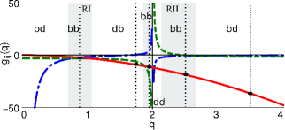
Figure 1: (Color online): Sketch showing the regions of existence of each type of solution, depending on different values of the parameter $q$. Dashed-dotted [blue] lines correspond to $g_{11}(q)$, solid [red] line to $g_{22}(q)$, and dashed [green] lines to $g_{12}(q)=g_{21}(q)$. Moreover vertical dashed [black] lines at $q=0.88$, $q=1.75$, $q=1.95$, $q=2.5$ and $q=3.5$ respectively, correspond to the parameters used for the simulations given below.

Table 1: Normalized amplitudes widths and frequencies

R	$(a_{2}/a_{1})^{2}\equiv\bar{a}$	$\left(\beta/a_{1}\right)^{2}\equiv\bar{\beta}$	$\left(\nu_{1}/a^{2}_{1}\right)$	$\left(\nu_{1}/\nu_{2}\right)$
$bb$	$\left(g_{11}-g_{21}\right)/\left(g_{22}-g_{12}\right)$	$\left(g_{12}^{2}-g_{11}g_{22}\right)/\left(g_{22}-g_{11}\right)$	$-\bar{\beta}/2$	$q$
$dd$	$\left(g_{11}-g_{21}\right)/\left(g_{22}-g_{12}\right)$	$\left(g_{11}g_{22}-g_{12}^{2}\right)/\left(g_{22}-g_{12}\right)$	$\bar{\beta}$	$q$
$db$	$\left(g_{11}-g_{21}\right)/\left(g_{12}-g_{22}\right)$	$\left(g_{12}^{2}-g_{11}g_{22}\right)/\left(g_{12}-g_{22}\right)$	$\bar{\beta}+g_{12}\bar{a}$	$2qg_{11}\left(g_{12}-g_{22}\right)$ $\left(g_{12}^{2}-2g_{12}g_{22}+g_{11}g_{22}\right)$
$bd$	$\left(g_{11}-g_{21}\right)/\left(g_{12}-g_{22}\right)$	$\left(g_{11}g_{22}-g_{12}^{2}\right)/\left(g_{12}-g_{22}\right)$	$-\bar{\beta}/2+g_{12}\bar{a}$	$-2qg_{11}\left(g_{12}-g_{22}\right)$ $\left(g_{12}^{2}-2g_{12}g_{22}+g_{11}g_{22}\right)$

The system of Eqs. (22)-(23), in the limit $g_{ij}=1$, is reduced to the integrable Manakov model manakov , which admits exact analytical solutions. For $g_{ij}\neq 1$ analytical soliton solutions of the CNLS system can also be obtained, as it was shown in a recent work veldes . In our case the coupling constants $g_{ij}$ depend on the parameter $q$ (cf. Fig. 1) and in general $g_{ij}\neq 1$. Adopting the method of veldes we show below that solitons can be obtained in different $q$ regions. First we look for solutions in the form of bright-bright ($bb$) solitons using the following ansatz:

$$f_{bb}=a_{1}{\rm sech}\left(\beta_{bb}x_{1}\right)e^{-i\nu_{1}t_{2}},$$ (25)

$$l_{bb}=a_{2}{\rm sech}\left(\beta_{bb}x_{1}\right)e^{-i\nu_{2}t_{2}},$$ (26)

where $a_{1,2}$ denote the amplitudes, $\nu_{1,2}$ the frequencies of the solitons, and $\beta_{bb}$ is the inverse width of the solitons. The condition that the squared amplitudes and widths of the solutions are positive defines three regions of the single parameter $q$ where $bb$ solitons can be found, i.e. $0.76<q<1.06$, $1.88<q<2$ and $2.13<q<2.63$. Another type of solution, in the form of dark-dark ($dd$) solitons, can also be obtained using the ansatz

$$f_{dd}=a_{1}\tanh\left(\beta_{dd}x_{1}\right)e^{-i\nu_{1}t_{2}},$$ (27)

$$l_{dd}=a_{2}\tanh\left(\beta_{dd}x_{1}\right)e^{-i\nu_{2}t_{2}}.$$ (28)

The aforementioned condition for the amplitudes and widths implies that solutions of this type are allowed in the region $2<q<2.13$. Finally, bright-dark ($bd$) vector soliton solutions ($f$, $l$) of the form:

$$f_{bd}=a_{1}{\rm sech}\left(\beta_{bd}x_{1}\right)e^{-i\nu_{1}t_{2}},$$ (29)

$$l_{bd}=a_{2}\tanh\left(\beta_{bd}x_{1}\right)e^{-i\nu_{2}t_{2}},$$ (30)

as well as dark-bright ($db$) solutions (by interchanging $f_{bd}\leftrightarrow l_{bd}$) can also be found. Solitons of the $bd$ ($db$) type are possible in the regions $0<q<0.76$, $q>2.63$ ($1.06<q<1.88$). In all cases the soliton widths, amplitudes and frequencies are connected through the equations shown in Table 1. Figure 1 shows the coupling constants $g_{ij}$ as functions of $q$, and the region of existence for each different vector soliton is highlighted. Using Eqs. (10)-(11) and the aforementioned soliton solutions of Eqs. (22)-(23) we can obtain localized approximate solutions (to order $\epsilon$) for the fields $A$ and $H$:

$$A(x,t) \approx 2\epsilon f(\epsilon\beta x)\cos\left[\left(1+\epsilon^{2}\nu_{1}\right)t\right],$$ (31)

$$H(x,t) \approx 2\epsilon l(\epsilon\beta x)\cos\left[\left(q+\epsilon^{2}\nu_{2}\right)t\right].$$ (32)

Inserting the profiles of $f$, $l$ in Eqs. (31)-(32), we obtain different classes of approximate solutions. Those corresponding to $bb$-solitons as in Eqs.(25)-(26), will have the form of oscillons for both fields. On the other hand $dd$-solitons correspond to solutions where both fields have the form of oscillating kinks. Finally $bd$ ($db$) solitons will result in an oscillon for the field $A$ ($H$) and an oscillating kink for $H$ ($A$).

II.3 Modulation Instability

In this section we will explore the impact of the modulation instability mechanism to the solution space of the Abelian-Higgs model. To this end, we examine the stability of plane wave solutions of the CNLS Eqs. (22)-(23). The mechanism of modulation instability (MI) mi is an important property of the NLS equation, revealing localized structures that a system supports, e.g. ${\rm sech}-shaped$ solutions of the form of Eqs. (25)-(26). This mechanism also gives information about the $\tanh-shaped$ solutions, e.g. Eqs. (27)-(28), since instability of plane waves leads to unstable background for this type of solutions. We consider the following ansatz:

$$f(x_{1},t_{2}) = \left(f_{0}+\delta f\right)e^{-i\Omega_{1}t_{2}},$$ (33)

$$l(x_{1},t_{2}) = \left(l_{0}+\delta l\right)e^{-i\Omega_{2}t_{2}},$$ (34)

where $f_{0}$ and $l_{0}$ are the amplitudes of the plane wave solutions of the CNLS equations, and $\Omega_{1,2}$ are their frequencies satisfying the dispersion relations

$$\omega_{1}\Omega_{1} = g_{11}|f_{0}|^{2}+g_{12}|l_{0}|^{2},$$ (35)

$$\omega_{2}\Omega_{2} = g_{21}|f_{0}|^{2}+g_{22}|l_{0}|^{2}.$$ (36)

The small amplitude perturbations i.e. $\delta f/f,\delta l/l\ll 1$, are complex functions of the form $\delta f=u_{1}+iw_{1}$, $\delta l=u_{2}+iw_{2}$. The real functions $u_{j},w_{j}$ are considered to be of the general form:

$$u_{j} = u_{0j}\exp[i\left(Kx_{1}-\Omega t_{2}\right)]+c.c.,$$ (37)

$$w_{j} = w_{0j}\exp[i\left(Kx_{1}-\Omega t_{2}\right)]+c.c.,$$ (38)

where the amplitudes $u_{0j}$, $w_{0j}$ are constants while K is the wavenumber and $\Omega$ the frequency of the perturbation. Substituting Eqs. (37)-(38) to the CNLS Eqs. (22)-(23) leads to an algebraic system of equations, the determinant of which has to be zero. This compatibility condition leads to the following equation:

$$A\Omega^{4}-\left(\omega^{2}_{1}B_{2}+\omega^{2}_{2}B_{1}\right)\Omega^{2}+\left(B_{1}B_{2}-\Gamma\right)=0,$$ (39)

where $A=\left(\omega_{1}\omega_{2}\right)^{2}$, $B_{j}=K^{2}/2\left(K^{2}/2+2g_{jj}f^{2}_{0}\right)$ with $j=1,2$ and $\Gamma=K^{4}g_{12}g_{21}(f_{0}l_{0})^{2}$. Requiring real roots of Eq. (39) we are led to the following stability conditions:

$$g_{11}g_{22}-g_{12}g_{21}>0,\quad g_{11}\geq 0,\quad g_{22}\geq 0.$$ (40)

As seen from Eq. (24), there are no real values of the parameter $q$ satisfying the last inequality of Eq. (40). Thus plane wave solutions are unstable under small perturbations. The aforementioned result implies that solutions including $d$ components, although they are allowed by the CNLS system in Eqs. (22)-(23), are expected to be unstable due to the modulation instability. This can be seen from the following fact: the dark-component in the solitons of Eqs. (27)-(30), takes asymptotically the form $\sim\pm a_{i}\exp[-i\nu_{i}t]$ at $x\rightarrow\pm\infty$. Hence away from its core, the solution is a plane wave and any perturbation will lead to the appearance of MI and the generation of oscillons. Thus we argue that localized solutions in the form of kinks, are not supported in the setting where $A$ and $H$ are of the same order.

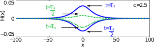
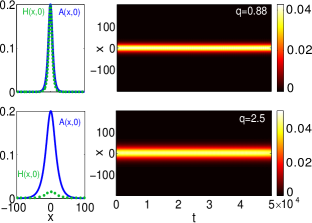
Figure 2: (Color online): Top panel shows a plot of the Higgs field for $t=T_{H}$, $t=T_{H}/2$ and $q=2.5$. Solid (blue) lines refer to the symmetric oscillations of the field $H(x)$. For comparison, in the same figure dotted (green) lines depict the oscillon in the asymmetric case. Middle-Bottom: left panels depict the profiles of the two fields $A$ [solid (blue) lines], and $H$ [dotted (green) line], for $t=0$, corresponding to oscillon solutions of Eqs. (31)-(32) for different values of $q$. Right panels: contour plots showing the evolution of the energy density $E(x,t)$ for initial conditions corresponding to the left panel. The total time of integration is $t=5\times 10^{4}$ and the different values of $q$ are depicted in the upper right corner of each contour.

According to the above analysis, the relevant solutions for the functions $f(x_{1},t_{2})$ and $l(x_{1},t_{2})$ are the $bb$ solitons, which are found in the three regions defined in the previous paragraph by Eqs. (25)-(26) (see also shaded areas of Fig. 1). The profile of a Higgs field oscillon with $q=2.5$, is shown in the top panel Fig. 2 with a solid (blue) line, for a half and a total period of oscillation. Notice that in contrast to previous findings prd , the Higgs field performs symmetric oscillations around the “classical vacuum”(i.e $H=0$). For comparison a typical solution of an asymmetric oscillon of Ref. prd is also shown in Fig. 2 [dotted (green) lines] for the same value of $q$. As already discussed, the two types of oscillons (asymmetric, symmetric) describe different scenarios for the underlying physics: the asymmetric solutions are valid in the case of weakly broken symmetry, i.e. just beyond the associated critical point, while the symmetric solutions occur when the gauge symmetry is strongly broken, i.e. far beyond the critical point.

It is also important to note that in the region $1.88<q<2$, the amplitudes of the second order expansions of the fields [cf. Eqs. (16)-(17)] become larger than $\mathcal{O}(1)$ and the perturbation scheme collapses. Thus, in this case oscillon solutions are not expected to exist for the exact system. However, our numerical results show that an initial condition corresponding to $bb$ solitons in this region also leads to robust oscillon solutions.

III Numerical results: oscillon’s longevity

According to the analysis of the previous section, robust localized solutions of the original system of equations (3)-(4) in the form of NLS bright-bright solitons, are expected to be found in the two parameter regions $0.76<q<1.06$ (RI) and $2.13<q<2.63$ (RII) [cf. Fig. 1]. To clarify this issue we perform numerical integration of the exact system Eqs. (3)-(4) for a wide range of $q$ values, using as initial conditions the approximate solutions Eqs. (31)-(32) for the case of bb-solitons. Our main interest is to confirm the existence of these structures and explore their long time dynamics. We use a fourth-order Runge-Kutta integrator for the time propagation with a lattice of length $L=400$, lattice spacing $dx=0.1$, time step $dt=10^{-2}$ and $\epsilon=0.1$. With this choice of parameters the numerical integration conserves the energy for the total time interval of our simulations up to the order of $10^{-3}$.

In the middle panel of Fig. 2 we show an example of the evolution of an oscillon in RI for $q=0.88$. The middle left panel depicts the oscillon profile at $t=0$, were solid (blue) line and dotted (green)line present $A$ and $H$ respectively. The evolution of the energy density $E(x,t)$ of Eq. 5, is shown in the middle right panel for a time interval of $t=5\times 10^{4}$, corresponding to $\sim 10^{4}$ oscillations for both fields. The energy density remains localized throughout the simulation, indicating the robustness of the oscillons in RI. We have confirmed (results not shown here) the existence and longevity of oscillons in this region for different values of $q$.

Next, an example of an oscillon in RII and for $q=2.5$ is shown in the bottom panels of Fig. 2. The evolution of the energy density in the right panel again confirms the existence of the respective oscillon solution and illustrates its longevity, since it turns out to be robust after performing at least $\sim 10^{4}$ oscillations. Note that for this example and for $q\in[2.3,2.63]$ (RII), the amplitude of $H$ gets suppressed so that the ratio of the amplitudes of the fields $H/A$ is close to the value of the perturbation parameter $\epsilon$. In this sense for this region of parameter values one recovers the scenario of small Higgs amplitude, explored in our previous work prd . However the solutions presented here have a different profile than those in prd . In particular, the Higgs field in prd exhibits asymmetric oscillations with respect to the origin (i.e. $H=0$), while the oscillon of Eq. (32) is symmetric [see also top panel of Fig. 2].

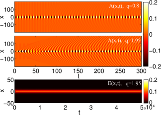
Figure 3: (Color online): Top and middle panels: Contour plots showing the evolution of the gauge field $A(x,t)$ for different values of $q$, as indicated in the upper right corner of each. Bottom: Contour of the energy density $E(x,t)$ for a time interval $t=5\times 10^{4}$.

Formally, this is due to the fact that the Higgs field in prd obeys a linear equation with an external source generated by the gauge field, while here the Higgs field obeys an NLS equation coupled with the gauge field. As previously explained, these two types of oscillons correspond to different scenarios for the underlying physics. We have performed simulations and confirmed the existence of robust oscillons described by Eqs. (25)-(26) in both RI and RII for various values of $q$.

Additionally, our numerical findings support the existence of oscillons in the region where the perturbation scheme is not valid, i.e. for $1.88<q<2$. Using the same initial condition as above, we have integrated Eqs. (3)-(4) for $q=1.95$ and the results are shown in the middle and bottom panels of Fig. 3. Since the system does not appear to support oscillons of the form of Eqs. (25)-(26), it is natural to expect a distortion of these type of solutions. Indeed, a large amount of radiation is emitted from the vicinity of the initially localized structure, as shown in the middle panel of Fig. 3. This panel depicts the short time evolution of $A$, and it is clearly seen that the distortion of the core starts very early. However, after sufficient time, a localized oscillating structure, different from the initial one, is formed and remains undistorted through the time of the evolution. The energy density of this oscillon is shown in the bottom panel of Fig. 3. The same qualitative result was observed for different values of $q$ in this region (results not shown here), suggesting that oscillons do exist but they are not described by Eqs. (25)-(26). For completeness, the short time evolution of an oscillon in RI is plotted in the top panel of Fig. 3, to highlight the fact that the radiation of the true oscillon solution (see Ref. segur ) has much smaller amplitude than the oscillon.

Next, we perform numerical integration of the exact system of equations in the regions of $q$ where solutions in the form of Eqs. (29)-(30) are expected to be subject to the MI mechanism.

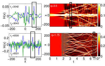
Figure 4: (Color online): Top left panel: profile snapshots of the field $H$ at two different instants, $t_{1}=3042$ dashed (blue) line and $t_{2}=3043$ solid (green) line. Solid (black) box focuses on a single oscillon showing its oscillation in half period. Top right panel: Contour plot showing the evolution of the energy density $E(x,t)$ for a $bd$ initial condition. The black box indicates the time of the snapshot. Bottom panels are the same as the top panels for plane wave initial conditions. In both contours the values of $q$ are indicated in the upper left corner, and the time interval is $t=7\times 10^{3}$.

The evolution of the energy density for such a $bd$ soliton is shown in the top right panel of Fig. 4 for $q=3.5$. We observe that at $t\sim 2\times 10^{3}$ the initially localized solution deforms and the instability settles in. Through the instability, localized structures occur on top of the initial solution (see e.g. the black box around $t=3042$) having the form of oscillons. As an example, the profile of the Higgs field for $t_{1}=3042$ [dashed (blue) line] and $t_{2}=3043$ [solid (green) line] is shown in the top left panel of Fig. 4. The solid (black) box indicates an oscillon performing a half oscillation period. The above result is in agreement with our analytical findings regarding the instability of the oscillating kinks.

We complete our numerical analysis by showing in the bottom panels of Fig. 4 the generation of oscillons at $q=1.75$, that is in the $db$ region. We have used initial conditions of the form: $A=H=C_{0}\left[1+\delta\cos(Kx)\right]$, where $C_{0}=0.05$ and $\delta=10^{-2}$ are the plane wave and the perturbation amplitude respectively and $K=0.025$ is a wavenumber inside the instability band given by Eq. (39). The initial, almost flat profile of the energy density deforms into a periodic pattern at $t\approx 2\times 10^{3}$, due to the modulational-instability-induced exponential growth of the wavenumber $K$. At later times moving oscillons are formed, which are subject to collisions and eventually some survive and some annihilate. The time interval indicated by the solid (black) box in the bottom right panel of Fig. 4 contains two time instants for which we show the Higgs field profile in the respective left panel. The solid (black) box in the left panel, focuses on a single oscillon at $x\approx 100$ performing a half oscillation period. Dashed (blue) line corresponds to $t_{1}=6530$ and solid (green) line to $t_{2}=6531$. The oscillon performs oscillations with period $T_{osc}=2\pi/q$ in agreement with the analytical predictions.

IV Conclusions and discussion

In conclusion, we have presented approximate analytical solutions of the $(1+1)$-dim Abelian- Higgs model, when the amplitudes of the gauge and the Higgs field are of the same order. Employing a multiple scale perturbation theory we reduced the original set of equations into a system of CNLS equations which admits different types of exact analytical solutions, depending on the parameter $q$ (i.e. the ratio of two field masses).

Our analysis reveals that bright-bright solitons of the CNLS equations lead to robust long-lived oscillon solutions of the original system. These oscillons are characterized by symmetric oscillations around the “classical vacuum”, for both the gauge and the Higgs field, describing excitations which may occur when the gauge symmetry is strongly broken (in contrast to the previous results of prd ).

Direct numerical simulations of the original system of equations of motion, confirm the robustness of the obtained solutions for times up to $5\times 10^{4}$ oscillation periods. These solutions are shown to exist in two different regions: $0.76<q<1.06$ (RI) and $2.13<q<2.63$ (RII). In the context of superconductor phenomenology a possible interpretation of our solutions is that oscillons with mass ratio less than unity (RI) correspond to type-I superconductors, while oscillons of RII, to type-II superconductors. This analogy is compatible with the statements reported in Ref. gleiser21 , for the Abelian-Higgs in $(3+1)$-dim.

Using the derived CNLS system we have also shown that for any value of the parameter $q$, plane waves are subject to the modulation instability mechanism. Dark-bright (bright-dark) solitons and the corresponding oscillating kinks were found to be unstable, and their instability was shown to lead into oscillon-like patterns.

The methodology used in the present work, may be applied in order to obtain novel localized structures in different settings, either with different potentials for the scalar field, or in the presence of non-Abelian gauge fields farhi05 and/or even in higher dimensional settings. Finally, based on the obtained solutions it would be interesting to further explore oscillon-oscillon interactions and understand their impact on the long time field dynamics.

References

- (1) E. J. Weinberg, Classical Solutions in Quantum Field Theory (Cambridge University Press, Cambridge, England, 2012); M. Gleiser, Int. J. Mod. Phys. D 16, 219 (2007); A. Rajantie, and E. J. Copeland, Phys. Rev. Lett. 85, 916 (2000).
- (2) M. A. Amin, R. Easther, H. Finkel, R. Flauger, and M. P. Hertzberg, Phys. Rev. Lett. 108, 241302 (2012).
- (3) N. Graham, and N. Stamatopoulos, Phys. Lett. B 639, 541 (2006); E. Farhi, N. Graham, A. H. Guth, N. Iqbal, R. R. Rosales, and N. Stamatopoulos, Phys. Rev. D 77, 085019 (2008).
- (4) R. V. Konoplich, S. G. Rubin, A. S. Sakharov, M. Yu. Khlopov, Phys. Atom. Nucl. 62, 1593 (1999); I. Dymnikova, L. Koziel, M. Khlopov, and S. Rubin, Grav. Cosmol. 6, 311 (2000); M. Yu. Khlopov, R. V. Konoplich, S. G. Rubin, and A. S. Sakharov, Grav. Cosmol. 6, 153 (2000).
- (5) M. Broadhead, J. McDonald, Phys. Rev. D 72, 043519 (2005); M. Gleiser, N. Graham, and N. Stamatopoulos, Phys. Rev. D 83, 096010 (2011).
- (6) M. Gleiser, and N. Graham, arXiv:1401.6225.
- (7) M. A. Amin, R. Easther, and H. Finkel, J. Cosmol. Astropart. Phys. 12 (2010) 001;M. A. Amin, and D. Shirokoff, Phys. Rev. D 81, 085045 (2010).
- (8) M. A. Amin, R. Easther, H. Finkel, R. Flauger, and M. P. Hertzberg, Phys. Rev. Lett. 108, 241302 (2012).
- (9) S. Khlebnikov, L. Kofman, A. Linde, and I. Tkachev, Phys. Rev. Lett. 81, 2012 (1998).
- (10) M. Gleiser, Int. J. Mod. Phys. D 16, 219 (2007); A. Rajantie, E. J. Copeland, Phys. Rev. Lett. 85, 916 (2000).
- (11) M. Gleiser, N. Graham, N. Stamatopoulos, Phys. Rev. D 82, 043517 (2010)
- (12) R. Rajaraman, Solitons and Instantons, (North-Holland, Amsterdam, 1982).
- (13) N. Manton, and P. Sutcliffe, Topological Solitons, (Cambridge University Press, 2004).
- (14) R. F. Dashen, B. Hasslacher, and A. Neveu, Phys. Rev. D 11, 3424 (1975).
- (15) I. L. Bogolyubskii, and V. G. Makhan’kov, [JETP Lett. 24, 12 (1976)]; I. L. Bogolyubskii, and V. G. Makhan’kov, JETP Lett. 25, 107 (1977).
- (16) G. Fodor, P. Forgács, Z. Horváth, and M. Mezei, Phys. Rev. D 79, 065002 (2009).
- (17) M. P. Hertzberg, Phys. Rev. D 82, 045022 (2010).
- (18) D. K. Campbell, J. F. Schonfeld, and C. A. Wingate, Physica, D 9, 1 (1983).
- (19) M. Hindmarsh, and P. Salmi, Phys. Rev. D 77, 105025 (2008).
- (20) M. Gleiser, and D. Sicilia, Phys. Rev. Lett. 101, 011602 (2008); M. Gleiser, D. Sicilia, Phys. Rev. D 80, 125037 (2009).
- (21) M. Gleiser, Phys. Lett. B 600, 126 (2004); P. M. Saffin, and A. Tranberg, JHEP 01, 030 (2007).
- (22) E. J. Copeland, M. Gleiser, and H. -R. Müller, Phys. Rev. D 52, 1920 (1995).
- (23) E.P. Honda, M.W. Choptuik, Phys. Rev. D 65, 084037 (2002).
- (24) G. Fodor, P. Forgács, and Z. Horváth, Á. Lukács, Phys. Rev. D 78, 025003 (2008).
- (25) M. A. Amin, Phys. Rev. D 87, 123505 (2013).
- (26) H. Segur, and M. D. Kruskal, Phys. Rev. Lett. 58, 747 (1987).
- (27) P. Arnold, and L. McLerran, Phys. Rev. D 37, 1020 (1988).
- (28) V. Achilleos, F. K. Diakonos, D. J. Frantzeskakis, G. C. Katsimiga, X. N. Maintas, E. Manousakis, C. E. Tsagkarakis, and A. Tsapalis, Phys. Rev. D 88, 045015 (2013).
- (29) M. Gleiser, and J. Thorarinson, Phys. Rev. D 79, 025016 (2009); M. Gleiser, and J. Thorarinson, Phys. Rev. D 76, 041701(R) (2007).
- (30) E. Farhi, N. Graham, V. Khemani, R. Markov, R. Rosales, Phys. Rev. D 72, 101701(R) (2005).
- (31) N. Graham, Phys. Rev. Lett. 98, 101801 (2007); N. Graham, Phys. Rev. D 76, 085017 (2007).
- (32) E.I. Sfakianakis, arXiv:hep-th/1210.7568.
- (33) S. Weinberg, The Quantum Theory of Fields: Volume II, (Cambridge University Press, 1996); M. D. Schwartz, Quantum Field Theory and the Standard Model, (Cambridge University Press, 2014).
- (34) L. P. Gork’ov, Sov. Phys. JETP 36, 1364 (1959); L. P. Gork’ov, and G. M. Eliashberg, Z. ksp. Teor. Fiz. 54, 612 (1968) [Sov. Phys. JETP 27, 328 (1968)]; V. L. Ginzburg, L. D. Landau, Zh. Eksp. Teor. Fiz. 20, 1064 (1950); A. A. Abrikosov, Zh. Eksp. Teor. Fiz. 32, 1442 (1957) [Sov. Phys. JETP 5, 1174 (1957)].
- (35) R. A. Ferrell, Phys. Rev. Lett. 13, 10 (1964); M. R. Bhagavan, J. Phys. C 2, 2 (1968); N. Dupuis, G. Montambaux, C. A. R. SÁ De Melo, Journal de Physique IV, 1993, 03 (C2), pp.C2-311-C2-314; E-W. Scheidt, C. Hauf, F. Reiner, G. Eickerling, and W. Scherer, J. Phys.: Conf. Ser. 273, 012083 (2011).
- (36) J. Ren JHEP 11, 055 (2010); X. Gao, M. Kaminski, H. B. Zeng, and H. Q. Zhang [arXiv:1204.3103]; H. B. Zeng, arXiv:1204.5325 [hep-th].
- (37) S. Raby, and A. Ukawa, Phys. Rev. D 18, 1154 (1978).
- (38) D. Yu. Grigoriev, V. A. Rubakov, and M. E. Shaposhnikov, Phys. Lett. B 216, 1 (1989); D. Yu. Grigoriev, and V . A. Rubakov, Nucl. Phys. B 299, 67 (1988); A. I. Bochkarev, and M. E. Shaposhnikov, Mod. Phys. Lett. A2, 991 (1987); W. H. Tang, and J. Smit, Nucl. Phys. B 540, 437 (1999); A. I. Bochkarev, and G. G. Tsitsishvili, Phys. Rev. D 40, 1378 (1989); J. Baacke, and N. Kevlishvili, Phys. Rev. D 78, 085008 (2008).
- (39) A. Jeffrey, T. Kawahara, Asymptotic methods in nonlinear wave theory, Pitman (1982).
- (40) X.N. Maintas, C.E. Tsagkarakis, F.K. Diakonos, D.J. Frantzeskakis, J. Mod. Phys. 3, 637 (2012), arXiv:hep-th/1306.6765; V. Achilleos, F.K. Diakonos, D.J. Frantzeskakis, G.C. Katsimiga, X.N. Maintas, C.E. Tsagkarakis, A. Tsapalis, Phys. Rev. D 85, 027702 (2012).
- (41) The destabilization of plane waves under small-amplitude long-wavelength perturbations is known as modulational instability or Benjamin-Feir instability [T.B. Benjamin and J.E. Feir, J. Fluid Mech. 27, 417 (1967)], and occurs in various contexts, including fluid mechanics [G.B. Whitham, J.Fluid Mech. 22, 273 (1965)], dielectrics [L.A. Ostrovsky, Sov. Phys. JETP 24, 797 (1967)], plasmas [A. Hasegawa, Phys. Fluids 15, 870 (1972)], etc.
- (42) S. V. Manakov, Zh. Eksp. Teor. Fiz. 65, 505 (1973) [Sov. Phys. JETP 38, 248 (1973)].
- (43) G.P. Veldes, J. Cuevas, P.G. Kevrekidis, D.J. Frantzeskakis, Phys. Rev. E 88, 013203 (2013).