Quantum spin correlations and random loops

Abstract.

We review the random loop representations of Tóth and Aizenman-Nachtergaele for quantum Heisenberg models. They can be combined and extended so as to include the quantum $XY$ model and certain SU(2)-invariant spin 1 systems. We explain the calculations of correlation functions.

1. Introduction

Random loop approaches to quantum spin systems offer an elegant and different perspective to quantum correlations. They find their origin in Feynman-Kac representations of quantum lattice systems. Motivated by earlier work of Conlon and Solovej [7], Tóth introduced a representation of the $S=\frac{1}{2}$ ferromagnetic Heisenberg model that is based on the random interchange model [17]. It allowed him to propose a bound for the free energy (it has been improved recently by Correggi, Giuliani, and Seiringer [8], who have reached the best possible constant). A similar representation was introduced by Aizenman and Nachtergaele for the $S=\frac{1}{2}$ antiferromagnet model [2] and certain models with higher spins. It allowed them to relate the one-dimensional quantum chain to two-dimensional Potts and random cluster models, yielding new insights on the quantum spin chain. This work was reviewed and extended in [15, 16]. See also [13] for a pedagogical introduction. Recently, Bachmann and Nachtergaele used the representation in their study of the classification of gapped ground states [4].

A synthesis of these two representations was proposed in [20]. In the case $S=\frac{1}{2}$, it applies to models that interpolate between the Heisenberg ferromagnetic and antiferromagnetic models such as the quantum $XY$ model. It also applies to certain SU(2)-invariant models of spin 1. Thanks to this representation, the existence of spin nematic long-range order was established in the model with $S=1$ in dimension $d\geq 3$ [20]. It also plays a rôle in the recent proof of emptyness formation of quantum spin chains of Crawford, Ng, and Starr [9].

This article reviews some of the material treated in [20], and also complements it. We consider the case of an external magnetic field, possibly disordered. We detail formulæ for the matrix elements of the operator $\,{\rm e}^{-\beta H}\,$ and use them to calculate correlation functions. Since there are few loop correlation functions, and seemingly more quantum spin correlation functions, the relations provide useful identities; these identities do not seem otherwise immediate.

2. Quantum spin models

Let $(\Lambda,{\mathcal{E}})$ be a graph, with $\Lambda$ the (finite) set of vertices and ${\mathcal{E}}$ the set of edges. Given $S\in\frac{1}{2}{\mathbb{N}}$, the Hilbert space is

$${\mathcal{H}}_{\Lambda}=\bigotimes_{x\in\Lambda}{\mathcal{H}}_{x},$$ (2.1)

where each ${\mathcal{H}}_{x}$ is a copy of ${\mathbb{C}}^{2S+1}$. The spin operators are denoted $S_{x}^{i}$, with $x\in\Lambda$ and $i=1,2,3$. They satisfy the commutation relations $[S_{x}^{1},S_{y}^{2}]={\rm i}\delta_{x,y}S_{x}^{3}$, and further relations obtained by cyclic permutations of the indices $1,2,3$. Recall that “classical configurations” $\sigma\in\{-S,\dots,S-1,S\}^{\Lambda}$ form a basis of ${\mathcal{H}}_{\Lambda}$ where the operators $S_{x}^{3}$ are diagonal: Using Dirac’s notation,

$$S_{x}^{3}|\sigma\rangle=\sigma_{x}|\sigma\rangle.$$ (2.2)

We consider the three operators $T_{xy}$, $P_{xy}$, $Q_{xy}$ on ${\mathcal{H}}_{\{x,y\}}$ (and their extensions on ${\mathcal{H}}_{\Lambda}$ by identifying $T_{xy}$ with $T_{xy}\otimes\mathrm{\texttt{Id}}_{\Lambda\setminus\{x,y\}}$, etc…):

• $T_{xy}$ is the transposition operator:

  $$T_{xy}|a,b\rangle=|b,a\rangle.$$ (2.3)

• $P_{xy}$ is the operator

  $$P_{xy}=\sum_{a,b=-S}^{S}(-1)^{a-b}|a,-a\rangle\langle b,-b|.$$ (2.4)

  Equivalently, the matrix coefficients of $P_{xy}$ are given by

  $$\langle a,b|P_{xy}|c,d\rangle=(-1)^{a-c}\delta_{a,-b}\delta_{c,-d}.$$ (2.5)

  Notice that $\frac{1}{2S+1}P_{xy}$ is the projector onto the spin singlet.

• $Q_{xy}$ is identical to $P_{xy}$ except for the signs:

  $$\langle a,b|Q_{xy}|c,d\rangle=\delta_{a,b}\delta_{c,d}.$$ (2.6)

These operators can be written in terms of spin operators. The form depends on the spin. In the case $S=\frac{1}{2}$, we have

$$\begin{split}&T_{xy}=2\bigl{(}S_{x}^{1}S_{y}^{1}+S_{x}^{2}S_{y}^{2}+S_{x}^{3}S_{y}^{3}\bigr{)}+\tfrac{1}{2},\\ &Q_{xy}=2\bigl{(}S_{x}^{1}S_{y}^{1}-S_{x}^{2}S_{y}^{2}+S_{x}^{3}S_{y}^{3}\bigr{)}+\tfrac{1}{2}.\end{split}$$ (2.7)

In the case $S=1$, we have

$$\begin{split}&T_{xy}=\vec{S}_{x}\cdot\vec{S}_{y}+(\vec{S}_{x}\cdot\vec{S}_{y})^{2}-1,\\ &P_{xy}=(\vec{S}_{x}\cdot\vec{S}_{y})^{2}-1.\end{split}$$ (2.8)

Here, we used the notation $\vec{S}_{x}\cdot\vec{S}_{y}=S_{x}^{1}S_{y}^{1}+S_{x}^{2}S_{y}^{2}+S_{x}^{3}S_{y}^{3}$.

Let ${\boldsymbol{h}}=(h_{x})_{x\in\Lambda}$ denote external magnetic fields. We consider two distinct families of Hamiltonians, indexed by the parameter $u\in[0,1]$:

$$H_{\Lambda,{\boldsymbol{h}}}^{(u)}=-\sum_{\{x,y\}\in{\mathcal{E}}}\Bigl{(}uT_{xy}+(1-u)Q_{xy}-1\Bigr{)}-\sum_{x\in\Lambda}h_{x}S_{x}^{3},$$ (2.9)

$$\tilde{H}_{\Lambda,{\boldsymbol{h}}}^{(u)}=-\sum_{\{x,y\}\in{\mathcal{E}}}\Bigl{(}uT_{xy}+(1-u)P_{xy}-1\Bigr{)}-\sum_{x\in\Lambda}h_{x}S_{x}^{3}.$$ (2.10)

Let $Z^{(u)}(\beta,\Lambda,{\boldsymbol{h}})$ and $\tilde{Z}^{(u)}(\beta,\Lambda,{\boldsymbol{h}})$ denote the corresponding partition functions:

$$Z^{(u)}(\beta,\Lambda,{\boldsymbol{h}})={\operatorname{Tr\,}}_{{\mathcal{H}}_{\Lambda}}\,{\rm e}^{-\beta H_{\Lambda,{\boldsymbol{h}}}^{(u)}}\,,$$ (2.11)

$$\tilde{Z}^{(u)}(\beta,\Lambda,{\boldsymbol{h}})={\operatorname{Tr\,}}_{{\mathcal{H}}_{\Lambda}}\,{\rm e}^{-\beta\tilde{H}_{\Lambda,{\boldsymbol{h}}}^{(u)}}\,.$$ (2.12)

The Hamiltonians of Eqs (2.9) and (2.10) can also be expressed in terms of spin operators. In the case $S=\frac{1}{2}$, we have

$$H_{\Lambda,{\boldsymbol{h}}}^{(u)}=-2\sum_{\{x,y\}\in{\mathcal{E}}}\bigl{(}S_{x}^{1}S_{y}^{1}+(2u-1)S_{x}^{2}S_{y}^{2}+S_{x}^{3}S_{y}^{3}-\tfrac{1}{4}\bigr{)}-\sum_{x\in\Lambda}h_{x}S_{x}^{3}.$$ (2.13)

The case $u=1$ is the Heisenberg ferromagnet. The case $u=\frac{1}{2}$ is the quantum XY model. If the graph is bipartite, the case $u=0$ is unitarily equivalent to the Heisenberg antiferromagnet.

In the case $S=1$, we have

$$\tilde{H}_{\Lambda,{\boldsymbol{h}}}^{(u)}=-\sum_{\{x,y\}\in{\mathcal{E}}}\Bigl{(}u\vec{S}_{x}\cdot\vec{S}_{y}+(\vec{S}_{x}\cdot\vec{S}_{y})^{2}-2\Bigr{)}-\sum_{x\in\Lambda}h_{x}S_{x}^{3}.$$ (2.14)

It is well-known that any two-body SU(2)-invariant interaction for $S=1$ can be be written as $J_{1}\vec{S}_{x}\cdot\vec{S}_{y}+J_{2}(\vec{S}_{x}\cdot\vec{S}_{y})^{2}$. The phase diagram of this model is very interesting and it has been investigated by several authors [5, 19, 18, 11]. It is displayed in Fig. 1. The line $J_{2}=0$ corresponds to the usual Heisenberg models.

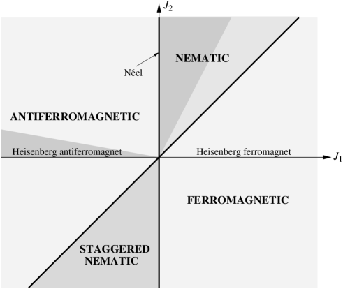
Figure 1. Phase diagram of the general spin 1 model with Hamiltonian $H=-\sum[J_{1}\vec{S}_{x}\cdot\vec{S}_{y}+J_{2}(\vec{S}_{x}\cdot\vec{S}_{y})^{2}]$, in dimension $d\geq 3$. The random loop representation applies to the half-quadrant $0\leq J_{1}\leq J_{2}$. The phase diagram is expected to show four phases (ferromagnetic, spin nematic, antiferromagnetic, staggered spin nematic). This is supported by rigorous results in the dark region around $J_{1}<0$ and small $J_{2}>0$ [10, 14], and in the dark region $0\leq J_{1}\leq\frac{1}{2}J_{2}$ [20].

3. Random loop models

Let us first describe the models of random loops. The connection to quantum spin systems will be described in the next two sections.

At each edge $\{x,y\}\in{\mathcal{E}}$ is attached the interval $[0,\beta]$ and a Poisson point measure where “crosses” occur with intensity $u$ and “double bars” occur with intensity $1-u$. Let $\omega$ denote a realization and $\rho({\rm d}\omega)$ denote independent Poisson point measures on ${\mathcal{E}}\times[0,\beta]$.

To a given realization $\omega$ of the Poisson point measure corresponds a set of loops, denoted ${\mathcal{L}}(\omega)$. The loops consist of vertical lines connected by crosses or bars. This is best understood by looking at pictures, see Fig. 2. A mathematically precise definition can be found in [20].

Figure 2. Graphs and realizations of Poisson point measures, and their loops. In both cases, the number of loops is $|{\mathcal{L}}(\omega)|=2$.

The relevant probability distribution involves multiplicative weights with respect to loops. We consider a function $w(\gamma)$ that assigns a real number to each loop $\gamma$. We will consider explicit weights below; for now, we just assume that $w(\gamma)$ depends on the loop in a continuous fashion, so all integrals below are well defined. In the case where $w(\gamma)$ is nonnegative for all $\gamma$ we have a probabilistic setting. But it is useful to include the possibility of negative weights as well.

We define the partition function as

$$Y(\beta,\Lambda)=\int\rho({\rm d}\omega)\prod_{\gamma\in{\mathcal{L}}(\omega)}w(\gamma).$$ (3.1)

We will always consider cases where $Y(\beta,\Lambda)\neq 0$. The relevant measure for the model of random loops is given by

$$\frac{1}{Y(\beta,\Lambda)}\,\Bigl{(}\prod_{\gamma\in{\mathcal{L}}(\omega)}w(\gamma)\Bigr{)}\,\rho({\rm d}\omega).$$ (3.2)

It is a probability measure when the weights are positive.

It is not hard to show that for $\beta$ small, and under some conditions on $w(\gamma)$, the loops have small lengths and the probability that two sites belong to the same loop shows exponential decay with respect to the distance between the sites. See e.g. Theorem 6.1 in [13].

The special case of constant weights, $w(\gamma)=\theta$, is interesting, and actually relevant to quantum systems without external magnetic fields. Under some additional assumptions, namely that the graph $(\Lambda,{\mathcal{E}})$ be a $d$-dimensional cube with even side lengths $L$ and $d\geq 3$, that $u\in[0,\frac{1}{2}]$, and that $\theta=2,3,\dots$, one can prove the existence of macroscopic loops when $\beta$ is sufficiently large. Let $\ell_{0}$ denote the random variable for the length of the loop that contains the point $(0,0)\in\Lambda\times[0,\beta]$. The length of the loop is defined as the sum of the length of all its vertical elements.

Theorem 1.

Under the assumptions listed in the paragraph above, there exists $c>0$ such that for all $L$,

$${\mathbb{E}}\Bigl{(}\frac{\ell_{0}}{\beta L^{d}}\Bigr{)}\geq c.$$

See [20, Chapter 5] for the statement with precise conditions. This theorem can be proved using the method of infrared bounds and reflection positivity introduced and developed in [12, 10, 14, 3]; see Biskup [6] for an excellent survey. This theorem implies the occurrence of long-range order in some quantum systems. The main novel result is the occurrence of spin nematic order for the spin 1 model with Hamiltonian $\tilde{H}_{\Lambda,{\boldsymbol{h}}}^{(u)}$ defined in Eq. (2.14). Indeed, it follows from Theorem 1 that

• $\displaystyle\frac{1}{|\Lambda|}\sum_{x}\langle S_{0}^{3}S_{x}^{3}\rangle>c$ for the model $H=-\sum(\vec{S}_{x}\cdot\vec{S}_{y})^{2}$, with $c>0$ independent of $\Lambda$, $d\geq 5$, $\beta$ large enough. (This is actually Néel order.)

• $\displaystyle\frac{1}{|\Lambda|}\sum_{x}\bigl{(}\langle(S_{0}^{3})^{2}(S_{x}^{3})^{2}\rangle-\langle(S_{0}^{3})^{2}\rangle\langle(S_{x}^{3})^{2}\rangle\bigr{)}>c$ for the model $H=-\sum\bigl{(}J_{1}\vec{S}_{x}\cdot\vec{S}_{y}+J_{2}(\vec{S}_{x}\cdot\vec{S}_{y})^{2}\bigr{)}$, with $c>0$ independent of $\Lambda$, $0\leq J_{1}\leq\frac{1}{2}J_{2}$, $d\geq 5$, $\beta$ large enough. (When $J_{1}\lesssim\frac{1}{2}J_{2}$ the result holds for $d\geq 3$.)

It does not seem possible to prove this using the method of infrared bounds and reflection positivity directly for quantum systems. The method in [20] consists in studying the model $H_{\Lambda}^{(u)}$, which is not related to $\tilde{H}_{\Lambda}^{(u)}$ in any obvious way when $u\neq 0,1$. The Gibbs operator $\,{\rm e}^{-\beta H_{\Lambda}^{(u)}}\,$ can be expanded in random loops and “space-time spin configurations” (see next section), which gives a sort of classical model that is reflection positive. This allows to prove “Gaussian domination”, leading to infrared bounds for the Duhamel two-point function. Combining with the Falk-Bruch inequality, as in [10, 14], one obtains Theorem 1. The results for $\tilde{H}_{\Lambda}^{(u)}$ are then consequences of the loop representation.

4. Gibbs operator and partition functions

The first result is a formula for the Gibbs operator $\,{\rm e}^{-\beta H}\,$ in terms of the Poisson point measure $\rho({\rm d}\omega)$. To a realization $\omega$ corresponds a sequence $(A_{1},t_{1}),\dots,(A_{n},t_{n})$ where $0<t_{1}<\dots<t_{n}<\beta$ are the times for the occurrence of events in $\omega$, and $A_{j}$ is the operator $T_{xy}$ if the event of time $t_{j}$ is a cross at $\{x,y\}\in{\mathcal{E}}$; $A_{j}$ is the operator $Q_{xy}$ if the event of time $t_{j}$ is a double bar at $\{x,y\}$.

Theorem 2.

We have

$$\,{\rm e}^{-\beta H_{\Lambda,{\boldsymbol{h}}}^{(u)}}\,=\int\rho({\rm d}\omega)\,{\rm e}^{-(\beta-t_{n})\sum h_{x}S_{x}^{3}}\,A_{n}\,{\rm e}^{-(t_{n}-t_{n-1})\sum h_{x}S_{x}^{3}}\,A_{n-1}\dots A_{1}\,{\rm e}^{-t_{1}\sum h_{x}S_{x}^{3}}\,.$$

The same representation applies to the operator $\,{\rm e}^{-\beta\tilde{H}_{\Lambda,{\boldsymbol{h}}}^{(u)}}\,$, but with $P_{xy}$ instead of $Q_{xy}$ when double bars occur. The proof can be done by discretizing the time interval $[0,\beta]$, linearizing the Poisson point measure, grouping terms wisely and invoking the Trotter product formula.

Next, we consider partition functions. Given a loop $\gamma$, we denote by $\ell_{x}(\gamma)$ the length of the vertical element(s) of the loop at site $x\in\Lambda$. We have $0\leq\ell_{x}(\gamma)\leq\beta$ and, for almost all realizations $\omega$,

$$\sum_{\gamma\in{\mathcal{L}}(\omega)}\sum_{x\in\Lambda}\ell_{x}(\gamma)=\beta|\Lambda|.$$ (4.1)

Theorem 3.

Given $S\in\frac{1}{2}{\mathbb{N}}$, let

$$w(\gamma)=\sum_{a=-S}^{S}\exp\Bigl{\{}a\sum_{x\in\Lambda}h_{x}\ell_{x}(\gamma)\Bigr{\}}.$$

Then for all $u\in[0,1]$, we have

$$Z^{(u)}(\beta,\Lambda,{\boldsymbol{h}})=\int\rho({\rm d}\omega)\prod_{\gamma\in{\mathcal{L}}(\omega)}w(\gamma).$$

In the case where $h_{x}\equiv 0$, we have $w(\gamma)=2S+1$ for all loops, and the partition function is equal to $\int(2S+1)^{|{\mathcal{L}}(\omega)|}\rho({\rm d}\omega)$.

The corresponding formula for the model with Hamiltonian $\tilde{H}_{\Lambda,{\boldsymbol{h}}}^{(u)}$ is more complicated, as it involves vertical directions of loops. Namely, let us choose an orientation for the loops, and let $\ell_{x}^{+}(\gamma)$ (resp. $\ell_{x}^{-}(\gamma)$) denote the vertical length of the elements of $\gamma$ at $x$ that move up (resp. that move down). We have $\ell_{x}^{+}(\gamma)+\ell_{x}^{-}(\gamma)=\ell_{x}(\gamma)$. We only state the theorem in the case of integer $S$, as there are inelegant signs when $S$ is half integer.

Theorem 4.

Given $S\in{\mathbb{N}}$, let

$$w(\gamma)=\sum_{a=-S}^{S}\exp\Bigl{\{}a\sum_{x\in\Lambda}h_{x}\bigl{[}\ell_{x}^{+}(\gamma)-\ell_{x}^{-}(\gamma)\bigr{]}\Bigr{\}}.$$

Then for all $u\in[0,1]$, we have

$$\tilde{Z}^{(u)}(\beta,\Lambda,{\boldsymbol{h}})=\int\rho({\rm d}\omega)\prod_{\gamma\in{\mathcal{L}}(\omega)}w(\gamma).$$

In order to prove Theorems 3 and 4, we need the concept of space-time configurations. This is also useful in the calculation of correlation functions. A space-time spin configuration is a function

$$\sigma:\Lambda\times[0,\beta]\longrightarrow\{-S,-S+1,\dots,S\}.$$ (4.2)

such that $\sigma_{x,t}$ is piecewise constant in $t$, for any $x$. Given a realization $\omega$ of the Poisson point measure, let $\Sigma_{\rm per}(\omega)$ denote the set of space-time spin configurations that take constant values along each loop. See Fig. 3 for an illustration. Let $\Sigma(\omega)$ denote the set of configurations that are compatible with $\omega$, but without requiring that $\sigma_{x,0}=\sigma_{x,\beta}$. Notice that

$$|\Sigma_{\rm per}(\omega)|=(2S+1)^{|{\mathcal{L}}(\omega)|}.$$ (4.3)

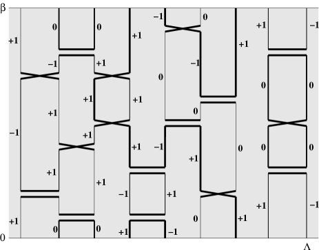
Figure 3. Illustration for a realization of the measure $\rho_{\iota}$ and a compatible space-time spin configuration.

We use Theorem 2 and we insert the resolution of the identity $\mathrm{\texttt{Id}}=\sum_{\sigma}|\sigma\rangle\langle\sigma|$ on the left of each transition $A_{j}$. Because of the definitions of $T_{xy}$ and $Q_{xy}$, we get

$$\begin{split}{\operatorname{Tr\,}}\,{\rm e}^{-\beta H_{\Lambda,{\boldsymbol{h}}}^{(u)}}\,&=\int\rho({\rm d}\omega)\sum_{\sigma\in\Sigma_{\rm per}(\omega)}\exp\Bigl{\{}-\sum_{x\in\Lambda}\int_{0}^{\beta}h_{x}\sigma_{x,t}{\rm d}t\Bigr{\}}\\ &=\int\rho({\rm d}\omega)\prod_{\gamma\in{\mathcal{L}}(\omega)}\sum_{a=-S}^{S}\,{\rm e}^{-a\sum_{x}h_{x}\ell_{x}(\gamma)}\,.\end{split}$$ (4.4)

This gives the claim of Theorem 3. The proof of Theorem 4 is similar but with different sets of space-time spin configurations. Let $\tilde{\Sigma}(\omega)$, $\tilde{\Sigma}_{\rm per}(\omega)$ with the prescription that the sign of the spin changes when the vertical direction of the loop changes. The calculation is then the same, with additional signs due to the double bars. Namely, a double bar at $\{x,y\}\times t$ gives the sign $(-1)^{\sigma_{x,t-}+\sigma_{x,t+}}$. Fortunately each loop involves an even number of minus signs, so the weight is positive.

5. Correlation functions

We restrict ourselves to two-point correlation functions. We also make the important simplification $h_{x}\equiv 0$, although expressions can certainly be derived for nonzero external magnetic fields. The loop correlations are given by just three events:

• $E_{x,y}^{+}$ is the set of all realizations $\omega$ such that $x$ and $y$ belong to the same loop, and with identical vertical direction at these points.

• $E_{x,y}^{-}$ is the set of all $\omega$ such that $x$ and $y$ belong to the same loop, and with opposite vertical directions at these points.

• $E_{x,y}=E_{x,y}^{+}\cup E_{x,y}^{-}$ is the set of all $\omega$ such that $x$ and $y$ belong to the same loop.

These events are illustrated in Fig. 4.

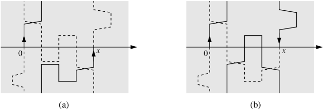
Figure 4. Illustration for (a) the event $E_{0,x}^{+}$; (b) the event $E_{0,x}^{-}$.

Let $A_{x}$ be an operator of the form $A\otimes\mathrm{\texttt{Id}}_{\Lambda\setminus\{x\}}$ and $B_{y}$ be an operator of the form $B\otimes\mathrm{\texttt{Id}}_{\Lambda\setminus\{y\}}$, where $A,B$ are operators on ${\mathbb{C}}^{2S+1}$. We consider the two-point function

$$\langle A_{x}B_{y}\rangle=\frac{1}{Z^{(u)}(\beta,\Lambda,0)}{\operatorname{Tr\,}}A_{x}B_{y}\,{\rm e}^{-\beta H_{\Lambda,0}^{(u)}}\,.$$ (5.1)

We use the notation ${\operatorname{tr\,}}$ for the trace in ${\mathbb{C}}^{2S+1}$. Let ${\mathbb{P}}(\cdot)$ denote the probability with respect to the random loop measure $Z^{(u)}(\beta,\Lambda,0)^{-1}(2S+1)^{|{\mathcal{L}}(\omega)|}\rho({\rm d}\omega)$.

Theorem 5.

For $x\neq y$, the correlation function above is given by

$$\langle A_{x}B_{y}\rangle=\tfrac{1}{2S+1}({\operatorname{tr\,}}AB)\;{\mathbb{P}}(E_{x,y}^{+})+\tfrac{1}{2S+1}({\operatorname{tr\,}}AB^{\rm t})\;{\mathbb{P}}(E_{x,y}^{-})+\tfrac{1}{(2S+1)^{2}}({\operatorname{tr\,}}A)({\operatorname{tr\,}}B)\;{\mathbb{P}}(E_{x,y}^{\rm c}).$$

Here, $B^{\rm t}$ denotes the transpose of the matrix $B$ in the basis where $\{S_{x}^{3}\}$ is diagonal. Choosing $B=\mathrm{\texttt{Id}}$, we get the formula for the one-point function (it is relevant for truncated correlation functions):

$$\langle A_{x}\rangle=\tfrac{1}{2S+1}{\operatorname{tr\,}}A.$$ (5.2)

An interesting special case of correlation function is $S=\frac{1}{2}$ and $A=B=S^{i}$. We find that

$$\langle S_{x}^{i}S_{y}^{i}\rangle=\begin{cases}\tfrac{1}{4}{\mathbb{P}}(E_{x,y})&\text{if }i=1,3,\\ \tfrac{1}{4}[{\mathbb{P}}(E_{x,y}^{+})-{\mathbb{P}}(E_{x,y}^{-})]&\text{if }i=2.\end{cases}$$ (5.3)

Proof of Theorem 5.

We use Theorem 2 and space-time spin configurations, and we get

$${\operatorname{Tr\,}}A_{x}B_{y}\,{\rm e}^{-\beta H_{\Lambda,0}^{(u)}}\,=\int\rho({\rm d}\omega)\sum_{\sigma\in\Sigma(\omega)}\langle\sigma_{\boldsymbol{\cdot},0}|A_{x}B_{y}|\sigma_{\boldsymbol{\cdot},\beta}\rangle.$$ (5.4)

Next we decompose

$$\int{\boldsymbol{\cdot}}\,\rho({\rm d}\omega)=\int_{E_{x,y}^{+}}{\boldsymbol{\cdot}}\,\rho({\rm d}\omega)+\int_{E_{x,y}^{-}}{\boldsymbol{\cdot}}\,\rho({\rm d}\omega)+\int_{E_{x,y}^{\rm c}}{\boldsymbol{\cdot}}\,\rho({\rm d}\omega)$$ (5.5)

and we treat each case separately. If $\omega\in E_{x,y}^{+}$, we find

$$\sum_{\sigma\in\Sigma(\omega)}\langle\sigma_{\boldsymbol{\cdot},0}|A_{x}B_{y}|\sigma_{\boldsymbol{\cdot},\beta}\rangle=(2S+1)^{|{\mathcal{L}}(\omega)|-1}\sum_{a,b=-S}^{S}\langle a,b|A_{x}B_{y}|b,a\rangle.$$ (5.6)

The term $(2S+1)^{|{\mathcal{L}}(\omega)|-1}$ is due to the sum of spin configurations on all the loops except the one that contains $x$ and $y$. The sum over $a,b$ represents the possible values of spins along this loop. Now we have

$$\langle a,b|A_{x}B_{y}|b,a\rangle=\langle a|A|b\rangle\langle b|B|a\rangle,$$ (5.7)

and the sum over $a,b$ gives ${\operatorname{tr\,}}AB$. The case where $\omega\in E_{x,y}^{-}$ is similar, but the matrix elements involving $A,B$ are

$$\langle a,a|A_{x}B_{y}|b,b\rangle=\langle a|A|b\rangle\langle a|B|b\rangle.$$ (5.8)

The sum over $a,b$ gives ${\operatorname{tr\,}}AB^{\rm t}$. Finally, the case $\omega\in E_{x,y}^{\rm c}$ involves two special loops, those containing $x$ and $y$, and we get

$$\sum_{\sigma\in\Sigma(\omega)}\langle\sigma_{\boldsymbol{\cdot},0}|A_{x}B_{y}|\sigma_{\boldsymbol{\cdot},\beta}\rangle=(2S+1)^{|{\mathcal{L}}(\omega)|-2}{\operatorname{tr\,}}A\;{\operatorname{tr\,}}B.$$ (5.9)

∎

The case of the Hamiltonian $\tilde{H}^{(u)}_{\Lambda,0}$ is more complicated due to the signs. They lead to signed measures when $S$ is half-integer but not integer (except when $u=0$ on a bipartite lattice). We restrict here to integer $S$ and we consider the two-point function

$$\langle A_{x}B_{y}\rangle^{\sim}=\frac{1}{\tilde{Z}^{(u)}(\beta,\Lambda,0)}{\operatorname{Tr\,}}A_{x}B_{y}\,{\rm e}^{-\beta\tilde{H}_{\Lambda,0}^{(u)}}\,.$$ (5.10)

We also write

$$\tilde{\mathbb{P}}(E_{x,y})=\frac{1}{\tilde{Z}^{(u)}(\beta,\Lambda,0)}\int 1_{E_{x,y}}(\omega)(2S+1)^{|{\mathcal{L}}(\omega)|}\,\rho({\rm d}\omega).$$ (5.11)

Theorem 6.

For $x\neq y$, the correlation above is given by

$$\begin{split}\langle A_{x}B_{y}\rangle^{\sim}=&\tfrac{1}{2S+1}({\operatorname{tr\,}}AB)\;\tilde{\mathbb{P}}(E_{x,y}^{+})+\tfrac{1}{2S+1}\biggl{(}\sum_{a,b=-S}^{S}(-1)^{a+b}\langle a|A|b\rangle\langle-a|B|-b\rangle\biggr{)}\;\tilde{\mathbb{P}}(E_{x,y}^{-})\\ &+\tfrac{1}{(2S+1)^{2}}({\operatorname{tr\,}}A)({\operatorname{tr\,}}B)\;\tilde{\mathbb{P}}(E_{x,y}^{\rm c}).\end{split}$$

The formula for one-point functions follow, $\langle A_{x}\rangle^{\sim}=\frac{1}{2S+1}{\operatorname{tr\,}}A$. The proof is similar to that of Theorem 5, but there are extra difficulties due to the minus signs. We do not write it explicitly. We find in particular (see [20] for more details)

$$\begin{split}&\langle S_{x}^{i}S_{y}^{i}\rangle=\tfrac{1}{3}S(S+1)\,\bigl{[}{\mathbb{P}}(E_{x,y}^{+})-{\mathbb{P}}(E_{x,y}^{-})\bigr{]}\\ &\langle(S_{x}^{i})^{2}(S_{y}^{i})^{2}\rangle-\langle(S_{x}^{i})^{2}\rangle\langle(S_{y}^{i})^{2}\rangle=\tfrac{1}{45}S(S+1)(2S-1)(2S+3)\,{\mathbb{P}}(E_{x,y}).\end{split}$$ (5.12)

It is remarkable that many spin correlation functions can be expressed with a handful of loop correlation functions.

Acknowledgments: I am grateful to Benjamin Lees for useful discussions. I would like to thank Pavel Exner, Wolfgang König, and Hagen Neidhardt, for organizing the conference QMATH 12 in Berlin, 10–13 September 2013, where this work was presented.

References

[1]
[2]
M. Aizenman, B. Nachtergaele,
Geometric aspects of quantum spin states,
Comm. Math. Phys., 164, 17–63 (1994)
[3]
C. Albert, L. Ferrari, J. Fröhlich, B. Schlein,
Magnetism and the Weiss exchange field — a theoretical analysis motivated by recent experiments,
J. Statist. Phys. 125, 77–124 (2006)
[4]
S. Bachmann, B. Nachtergaele,
On gapped phases with a continuous symmetry and boundary operators,
J. Statist. Phys. 154, 91–112 (2014)
[5]
C.D. Batista, G. Ortiz,
Algebraic approach to interacting quantum systems,
Adv. Phys. 53, 1–82 (2004)
[6]
M. Biskup,
Reflection positivity and phase transitions in lattice spin models,
in Methods of contemporary mathematical statistical physics, Lect. Notes Math. 1970, 1–86 (2009)
[7]
J. Conlon, J.P. Solovej,
Upper bound on the free energy of the spin 1/2 Heisenberg ferromagnet,
Lett. Math. Phys. 23, 223–231 (1991)
[8]
M. Correggi, A. Giuliani, R. Seiringer,
Validity of the spin-wave approximation for the free energy of the Heisenberg ferromagnet,
arXiv:1312.7873 [math-ph] (2013)
[9]
N. Crawford, S. Ng, S. Starr,
in preparation
[10]
F.J. Dyson, E.H. Lieb, B. Simon,
Phase transitions in quantum spin systems with isotropic and nonisotropic interactions,
J. Statist. Phys. 18, 335–383 (1978)
[11]
Yu.A. Fridman, O.A. Kosmachev, Ph.N. Klevets,
Spin nematic and orthogonal nematic states in non-Heisenberg magnet,
J. Magnetism and Magnetic Materials 325, 125–129 (2013)
[12]
J. Fröhlich, B. Simon, T. Spencer,
Infrared bounds, phase transitions and continuous symmetry breaking,
Comm. Math. Phys. 50, 79–95 (1976)
[13]
C. Goldschmidt, D. Ueltschi, P. Windridge,
Quantum Heisenberg models and their probabilistic representations,
in Entropy and the Quantum II, Contemp. Math. 552, 177–224 (2011); arXiv:1104.0983 [math-ph]
[14]
T. Kennedy, E.H. Lieb, B.S. Shastry,
Existence of Néel order in some spin- Heisenberg antiferromagnets,
J. Statist. Phys. 53, 1019–1030 (1988)
[15]
B. Nachtergaele,
Quasi-state decompositions for quantum spin systems,
in Probability Theory and Mathematical Statistics, B Grigelionis et al (eds),
pp 565–590 (1994);
arXiv:cond-mat/9312012
[16]
B. Nachtergaele,
A stochastic geometric approach to quantum spin systems,
in Probability and Phase Transitions, G. Grimmett (ed.), Nato Science series C 420, pp 237–246 (1994)
[17]
B. Tóth,
Improved lower bound on the thermodynamic pressure of the spin Heisenberg ferromagnet,
Lett. Math. Phys. 28, 75–84 (1993)
[18]
T.A. Tóth, A.M. Läuchli, F. Mila, K. Penc,
Competition between two- and three-sublattice ordering for spins on the square lattice,
Phys. Rev. B 85, 140403 (2012)
[19]
H.-H. Tu, G.-M. Zhang, T. Xiang,
Class of exactly solvable SO(n) symmetric spin chains with matrix product ground states,
Phys. Rev. B 78, 094404 (2008)
[20]
D. Ueltschi,
Random loop representations for quantum spin systems,
J. Math. Phys. 54, 083301 (2013)