Contribution of plasminos to the shear viscosity of a
hot and dense Yukawa-Fermi gas

Abstract

We determine the shear viscosity of a hot and dense Yukawa-Fermi gas, using the standard Green-Kubo relation, according to which the shear viscosity is given by the retarded correlator of the traceless part of viscous energy-momentum tensor. We approximate this retarded correlator using a one-loop skeleton expansion, and express the bosonic and fermionic shear viscosities, $\eta_{b}$ and $\eta_{f}$, in terms of bosonic and fermionic spectral widths, $\Gamma_{b}$ and $\Gamma_{\pm}$. Here, the subscripts $\pm$ correspond to normal and collective (plasmino) excitations of fermions. We study, in particular, the effect of these excitations on thermal properties of $\eta_{f}[\Gamma_{\pm}]$. To do this, we determine first the dependence of $\Gamma_{b}$ and $\Gamma_{\pm}$ on momentum $p$, temperature $T$, chemical potential $\mu$ and $\xi_{0}\equiv m_{b}^{0}/m_{f}^{0}$, in a one-loop perturbative expansion in the orders of the Yukawa coupling. Here, $m_{b}^{0}$ and $m_{f}^{0}$ are $T$ and $\mu$ independent bosonic and fermionic masses, respectively. We then numerically determine $\eta_{b}[\Gamma_{b}]$ and $\eta_{f}[\Gamma_{\pm}]$, and study their thermal properties. It turns out that whereas $\Gamma_{b}$ and $\Gamma_{+}$ decrease with increasing $T$ or $\mu$, $\Gamma_{-}$ increases with increasing $T$ or $\mu$. This behavior qualitatively changes by adding thermal corrections to $m_{b}^{0}$ and $m_{f}^{0}$, while the difference between $\Gamma_{+}$ and $\Gamma_{-}$ keeps increasing with increasing $T$ or $\mu$. Moreover, $\eta_{b}$ ($\eta_{f}$) increases (decreases) with increasing $T$ or $\mu$. We show that the effect of plasminos on $\eta_{f}$ becomes negligible with increasing (decreasing) $T$ ($\mu$).

I Introduction

One of the main goals of the modern experiments of ultra-relativistic heavy ion collisions is to clarify the nature of the phase transition of quantum chromodynamics (QCD). As predicted from numerical computations on the lattice, at a temperature of about $150$ MeV, quark matter undergoes a phase transition, during which hadrons melt and a new state of matter, a plasma of quarks and gluons is built. There are strong evidences for the creation of the Quark-Gluon Plasma (QGP) in heavy ion experiments at the Relativistic Heavy-Ion Collider (RHIC) and the Large Hadron Collider (LHC) STARcollab . The experimental results show that the elliptic flow, $v_{2}$, describing the azimuthal asymmetry in momentum space, is the largest ever seen in heavy ion collisions kapusta2008 . The elliptic flow $v_{2}$ is proportional to the initial eccentricity $\epsilon_{2}\equiv|\langle r^{2}e^{2i\phi}\rangle|/\langle r^{2}\rangle$ of a given collision, that describes the asymmetric region of overlap in a collision between two nuclei and results in an anisotropy in the transverse density of the system at the early stages of the collision ollitrault2012 . The collective response of the system, well described by viscous hydrodynamics, transforms this spatial anisotropy into a momentum anisotropy. Thus, $v_{2}$ is proportional to $\epsilon_{2}$, with the proportionality factor depending on the shear viscosity $\eta$ of the medium ollitrault2012 . The latter characterizes the diffusion of momentum transverse to the direction of propagation. The comparison between the experimentally measured $v_{2}$ and the results arising from second order viscous hydrodynamics has suggested that the new state of matter created at RHIC and LHC is an almost perfect fluid, having a very small shear viscosity to entropy density ratio $\eta/s$ heinz2001 ; romatschke2007 (see also song2012 for a recent review on the status of $\eta/s$). However, as is reported in song2012 , in all hydrodynamic simulations performed so far, the shear viscosity is assumed to be temperature independent.

The shear viscosity is one of the transport coefficients, which describe the properties of a system out of equilibrium, and can theoretically be determined using two different approaches: The kinetic theory approach, based on the Boltzmann equation for the corresponding momentum distribution function kineticapproach ; redlich2008 ; ghosh2013 , and the Green-Kubo approach in the framework of linear response theory green-kubo , in which all transport coefficients are formulated in terms of retarded correlators of the energy-momentum tensor jeon1994 ; kuboapproach . The advantage of the second method is, that it provides a framework, where the transport coefficients can be computed using equilibrium thermal field theory. Other alternative methods to compute transport coefficients are direct numerical simulations on a space-time lattice aartslattice , using two-Particle Irreducible (2PI) effective action aarts2PI , and holographic models kovtun2004 . A novel diagrammatic method is also presented in hidaka2010 . The aim of the most of these computations is to determine the dependence of $\eta$ on temperature and chemical potential nardi2009 ; lang2012 ; lang2013 or on external electromagnetic fields nam2013 .

In this paper, we use the Green-Kubo formalism to determine the dependence of the shear viscosity of a Yukawa-Fermi gas on temperature, chemical potential, and bosonic and fermionic masses. Thermal corrections to the masses of bosons and fermions will be considered too and their effect on the shear viscosity will be scrutinized. Our approach is similar to what is recently presented by Lang et al. in lang2012 ; lang2013 . In lang2012 , an appropriate skeleton expansion is used to approximate the retarded correlators appearing in the Kubo relation for the shear viscosities of a real $\lambda\varphi^{4}$ theory and an interacting pion gas. Using the standard Källen-Lehmann representation of retarded two-point Green’s function in term of interacting bosonic spectral function, $\rho_{b}$, the shear viscosity of the scalar and pseudo-scalar bosons, $\eta_{b}$, is then expressed in terms of the real and imaginary part of the retarded two-point Green’s function. The latter, denoted by $\Gamma_{b}$, defines, in particular, the spectral width of the bosons and is inversely proportional to their mean free-path. To approximate the bosonic correlators, a systematic Laurent expansion of $\eta_{b}$ in the orders of $\Gamma_{b}$ is performed. The series is then truncated in the leading $\Gamma_{b}^{-1}$ order. Computing then $\Gamma_{b}$ perturbatively in the orders of the small coupling constant of the theory, up to the first non-vanishing contribution, the $T$ dependence of bosonic shear viscosity is numerically determined. In lang2013 , almost the same method is used to determine the fermionic shear viscosity, $\eta_{f}$, of a strongly interacting quark matter, described by a two-flavor Nambu–Jona-Lasinio (NJL) model NJL , that consists of a four-fermion interaction with no gluons involved. To do this, $\eta_{f}$ is first expressed in terms of fermionic spectral function, $\rho_{f}$, and then working, as in iwasaki2006 , in a quasiparticle approximation, a generalized Breit-Wigner shape for the fermionic spectral function is used to formulate $\eta_{f}$ in terms of quasiparticle mass $M$ and width $\Gamma_{f}$. Using then four different parameterizations for $\Gamma_{f}$, the thermal properties of $\eta_{f}$ is explored. Eventually, the constant quasiparticle mass $M$ is replaced with $T$ and $\mu$ dependent, dynamically generated constituent quark mass of the NJL model, and the thermal properties of $\eta_{f}$ are qualitatively studied in the vicinity of the chiral transition point.

In the present paper, we will compute the shear viscosity of an interacting boson-fermion system with Yukawa coupling. In this theory, the shear viscosity consists of a bosonic and a fermionic part. Following the method presented in lang2012 , we will first derive $\eta_{b}$ in term of $\Gamma_{b}$ in a systematic Laurent expansion up to ${\cal{O}}(\Gamma_{b}^{0})$. Performing then a one-loop perturbative expansion in the orders of the Yuwaka coupling, we will determine $\Gamma_{b}$ as a function of momentum $p$, temperature $T$, chemical potential $\mu$ and $\xi_{0}\equiv m_{b}^{0}/m_{f}^{0}$, where $m_{b}^{0}$ and $m_{f}^{0}$ are constant bosonic and fermionic masses. Using $\eta_{b}[\Gamma_{b}]$, we will study the $T$ and $\mu$ dependence of the bosonic shear viscosity for various $\xi_{0}$. We will then add the thermal masses of bosons and fermions to $m_{b}^{0}$ and $m_{f}^{0}$, and study the effect of thermal masses on $\Gamma_{b}$ and $\eta_{b}$. Thermal corrections to the masses of bosons and fermions are computed using standard Hard Thermal Loop (HTL) method (see e.g. in kiessig2010 ). Let us notice that, according to the description in kiessig2009 , this ad-hoc treatment of thermal masses seems intuitive and is justified, since it equals the HTL treatment with an approximate fermion propagator. However, it is not equal the full HTL result kiessig2010 .

We will then focus on the fermionic part of the shear viscosity, and derive its dependence on the fermionic spectral width. This build the central part of the analytical results of the present paper. Here, in contrast to the approximations made in lang2013 , we use the spectral representation of retarded two-point Green’s function presented for the first time in weldon1989 (see also weldon1999 ). The latter is used in kiessig2010 ; plasmino-app ; blaizot1996 ; jeon2007 ; plasmino-NJL ; plasmino-QED ; plasmino-QCD ; plasmino-yukawa-1 ; plasmino-yukawa-2 ; balizot2014 within the context of Yukawa theory, NJL model, QED and QCD. In weldon1989 , it is shown that a fermionic system at finite temperature has twice as many fermionic modes as at zero temperature. Besides propagating quark and antiquarks, there are also propagating quark holes and antiholes. Thus, thermal fermions have, apart from normal excitation, a collective excitation, referred to either as a hole or as a plasmino weldon1999 . The latter appears as an additional pole in the fermion propagator, and as a consequence of the preferred frame defined by the heat bath. Hence, the two poles lead to two different dispersion relations, both with positive energy. It turns out that in the chiral limit $m_{f}^{0}\to 0$, the normal excitation has the same chirality and helicity, while the collective excitation possesses opposite chirality and helicity weldon1999 . Denoting the spectral widths, corresponding to the normal and collective (plasmino) excitations, with $\Gamma_{+}$ and $\Gamma_{-}$, respectively, we will use the aforementioned Laurent expansion to derive a novel analytic relation for $\eta_{f}$ in term of $\Gamma_{\pm}$ up to ${\cal{O}}(\Gamma_{\pm}^{0})$. We will then determine the $p$, $T$, $\mu$ and $\xi_{0}$ dependence of $\Gamma_{\pm}$ in a one-loop perturbative expansion in the orders of the Yukawa coupling. Using $\eta_{f}[\Gamma_{\pm}]$, it is then possible to explore the thermal properties of $\eta_{f}$ for various $\xi_{0}$. Adding thermal corrections to the bosonic and fermionic masses, the effect of thermal masses on $\Gamma_{\pm}$ and $\eta_{f}$ will be also studied. Let us notice at this stage that in the literature nardi2009 ; jeon2007 ; plasmino-yukawa-1 , the difference between $\Gamma_{+}$ and $\Gamma_{-}$, as well as their $p$ dependence are often neglected, and $\Gamma_{\pm}(p)$ is approximated by $\Gamma_{\pm}(0)\propto g^{2}T$, where $g$ is the coupling constant of the theory nardi2009 ; plasmino-yukawa-1 . We, however, will explicitly determine the $p$-dependence of $\Gamma_{+}$ and $\Gamma_{-}$, and use it in the numerical computation of $\eta_{f}$. Then, we will assume $\Gamma_{+}=\Gamma_{-}$, and will determine the difference between $\eta_{f}[\Gamma_{+}\neq\Gamma_{-}]$ and $\eta_{f}[\Gamma_{+}=\Gamma_{-}]$ in terms of $T$ and $\mu$. It turns out that, depending on $T$ and/or $\mu$, $\eta_{f}[\Gamma_{+}=\Gamma_{-}]$ is larger than $\eta_{f}[\Gamma_{+}\neq\Gamma_{-}]$.

The organization of this paper is a follows: In Sec. II, we will review the Green-Kubo formalism, and present the shear viscosity in terms of retarded correlators of the traceless part of the viscous energy-momentum tensor. In Sec. III, we start with the Lagrangian density of the Yukawa theory, and derive the bosonic and fermionic contributions to the shear viscosity, in a one-loop skeleton expansion, in terms of bosonic and fermionic spectral density functions, $\rho_{b}$ and $\rho_{f}$. Eventually, using an appropriate Laurent expansion in the orders of bosonic and fermionic spectral widths, $\eta_{b}[\Gamma_{b}]$ and $\eta_{f}[\Gamma_{\pm}]$ are determined (see Secs. III.1 and III.2 as well as Apps. A and C). In Sec. IV, the spectral bosonic and fermionic widths, $\Gamma_{b}$ and $\Gamma_{\pm}$ are separately computed in one-loop perturbative expansion in the orders of the Yukawa coupling (see Sec. IV.1 for the bosonic and Sec. IV.2 for the fermionic spectral widths). In order to derive the imaginary part of the retarded two-point Green’s functions, corresponding to bosons and fermions, the standard Schwinger-Keldysh real-time formalism schwinger1961 is used. We will mainly use the notations of dasbook and kobes1985 . In Sec. V, we will present our numerical results. Here, the $T,\mu$ and $\xi_{0}$ dependence of $\Gamma_{b}$ and $\Gamma_{\pm}$, as well as the thermal properties of $\eta_{b}[\Gamma_{b}]$ and $\eta_{f}[\Gamma_{\pm}]$, will be explored. As it turns out, $\Gamma_{b}$ and $\Gamma_{+}$ decreases with increasing $T$ or $\mu$. In contrast, $\Gamma_{-}$ increases with increasing $T$ or $\mu$. Whereas this behavior changes when thermal corrections are added to $m_{b}^{0}$ and $m_{f}^{0}$, $\Gamma_{+}$ and $\Gamma_{-}$ still exhibit different $T$ and $\mu$ dependence. This difference increases with increasing $T$ or $\mu$. As concerns the shear viscosities, $\eta_{b}$ ($\eta_{f}$) increases (decreases) with increasing $T$ or $\mu$. Moreover, it turns out that the contribution of plasminos on $\eta_{f}$ becomes negligible with increasing (decreasing) $T$ ($\mu$). A summary of our results is presented in Sec. VI.

II Shear Viscosity in Relativistic Hydrodynamics

An ideal and locally equilibrated relativistic fluid is mainly described by the dynamics of the corresponding energy-momentum tensor

$$T^{\mu\nu}_{0}=\epsilon\hskip 0.56917ptu^{\mu}u^{\nu}+P\hskip 0.56917pt\Delta^{\mu\nu},$$ (II.1)

where $\epsilon$ is the energy density, $P$ the pressure and $u_{\mu}(x)=\gamma(x)(1,\mathbf{v}(x))$ is the four velocity of the fluid, which is defined by the variation of the four-coordinate $x^{\mu}$ with respect to the proper time $\tau$. Here, the Lorentz factor $\gamma(x)\equiv(1-\mathbf{v}^{2}(x))^{-1}$. In (II.1), $\Delta^{\mu\nu}$ is defined by $\Delta^{\mu\nu}\equiv g^{\mu\nu}-u^{\mu}u^{\nu}$, with the metric $g^{\mu\nu}=\mbox{diag}\left(+,-,-,-\right)$. It satisfies $u_{\mu}\Delta^{\mu\nu}=0$. Moreover, for the four-velocity $u_{\mu}$, we have $u_{\mu}u^{\mu}=1$. If there are no external sources, the energy-momentum tensor (II.1) is conserved

$$\partial_{\mu}T^{\mu\nu}_{0}=0.$$ (II.2)

Apart from (II.2), an ideal fluid is characterized by the entropy current conservation law $\partial_{\mu}s^{\mu}=0$, where the entropy current, $s_{\mu}\equiv su_{\mu}$, includes the entropy density $s$. In a system without conserved charges, $\epsilon$ and $P$ satisfy $\epsilon+P=Ts$, where $T$ is the local temperature of the fluid.

To include dissipative effects to the fluid, the viscous-stress tensor $\tau^{\mu\nu}$ is to be added to $T_{0}^{\mu\nu}$ from (II.1). The total energy-momentum tensor then reads

$$T^{\mu\nu}=T^{\mu\nu}_{0}+\tau^{\mu\nu},$$ (II.3)

where $\tau^{\mu\nu}$ satisfies $u_{\mu}\tau^{\mu\nu}=0$. In an expansion in the orders of derivatives of $u_{\mu}$, the viscous stress tensor is determined using the second law of thermodynamics, $T\partial_{\mu}s^{\mu}\geq 0$, that replaces the conservation law $\partial_{\mu}s^{\mu}=0$ of the ideal fluid. The viscous stress tensor is often split as

$$\tau^{\mu\nu}=\pi^{\mu\nu}+\Delta^{\mu\nu}\Pi,$$ (II.4)

where $\pi^{\mu\nu}$ is the traceless part ($\pi^{\mu}_{~{}\mu}=0$) and $\Pi$ is the remaining part with non-vanishing trace. Each part of $\tau^{\mu\nu}$ is then parameterized by a number of viscous coefficients. In the first order derivative expansion, $\tau^{\mu\nu}$ is characterized by the shear and bulk viscosities, $\eta$ and $\zeta$, that appear in the traceless part of $\tau^{\mu\nu}$,

$$\pi^{\mu\nu}=\eta\left(\nabla^{\mu}u^{\nu}+\nabla^{\nu}u^{\mu}-\frac{2}{3}\Delta^{\mu\nu}\nabla^{\rho}u_{\rho}\right),$$ (II.5)

and in the part of $\tau^{\mu\nu}$ with non-vanishing trace,

$$\Pi=\zeta\nabla^{\mu}u_{\mu},$$ (II.6)

respectively. Here, $\nabla^{\mu}\equiv\Delta^{\mu\nu}\partial_{\nu}$. Using the properties of $\Delta^{\mu\nu}$ in $d=4$ dimensional space-time, $\Delta^{\mu\nu}u_{\nu}=0$ as well as $\Delta^{\rho}_{\mu}\Delta^{\mu}_{~{}\nu}=\Delta^{\rho}_{~{}\nu}$, we get

$$\epsilon=u_{\mu}u_{\nu}T^{\mu\nu},\qquad P=-\frac{1}{3}\Delta_{\mu\nu}T^{\mu\nu},$$ (II.7)

as well as

$$\tilde{\pi}^{\mu\nu}=\left(\Delta^{\rho\mu}\Delta^{\sigma\nu}+\Delta^{\rho\nu}\Delta^{\sigma\mu}-\frac{2}{3}\Delta^{\mu\nu}\Delta^{\rho\sigma}\right)T_{\rho\sigma}.$$ (II.8)

Here, $\tilde{\pi}^{\mu\nu}\equiv\eta^{-1}\pi^{\mu\nu}$ is introduced. In the rest of this paper, we will focus on the shear viscosity $\eta$. Following Zubarev’s approach green-kubo and within linear response theory, it is determined by the Kubo-type formula lang2012

$$\eta=\frac{\beta_{s}}{10}\int d^{3}x^{\prime}\int_{-\infty}^{t}dt^{\prime}\left(\tilde{\pi}^{\mu\nu}(0),\tilde{\pi}_{\mu\nu}(\mathbf{x}^{\prime},t^{\prime})\right),$$ (II.9)

where the inverse proper temperature $\beta_{s}\equiv\gamma\beta$ with $\beta\equiv T^{-1}$, and

$$\left(X,Y\right)=\frac{1}{\beta}\int_{0}^{\beta}d\tau\langle X[~{}e^{H\tau}Ye^{-H\tau}-\langle Y\rangle_{0}~{}]\rangle_{0}.$$ (II.10)

Here, $H$ is the free part of the Hamiltonian of a fully interacting theory, which is given in terms of the energy momentum tensor $T^{\mu\nu}$, via $\beta H=\int d^{3}x\beta_{s}(\mathbf{x},\tau)u^{\mu}(\mathbf{x},\tau)T_{0\mu}(\mathbf{x},\tau)$. Moreover, $\langle\cdots\rangle_{0}$ is the thermal expectation value with respect to the equilibrium statistical operator $\rho_{0}$, and is defined by $\langle\cdot\rangle_{0}=\mbox{tr}(\cdot\rho_{0})$ lang2012 . The correlator appearing in (II.9) can be expressed as a real-time integral over a retarded correlator

$$\left(X(t),Y(t^{\prime})\right)\sim-\frac{1}{\beta}\int_{-\infty}^{t^{\prime}}dt^{\prime\prime}\langle X(t),Y(t^{\prime\prime})\rangle_{R},$$ (II.11)

with

$$\langle X(t),Y(t^{\prime})\rangle_{R}=-i\theta(t-t^{\prime})\langle\big{[}X(t),Y(t^{\prime})\big{]}\rangle_{0}.$$ (II.12)

In the large-time limit $t^{\prime}\to\infty$, when the system approaches global equilibrium, the approximation appearing in (II.11) becomes exact. Combining at this stage (II.9) and (II.11), and evaluating the resulting expression in the local rest-frame, where $\beta_{s}=\beta$, the Kubo-formula for the shear viscosity reads

$$\eta=-\frac{1}{10}\int_{-\infty}^{0}dt\int_{-\infty}^{t}dt^{\prime}~{}\Pi_{R}(t^{\prime}),$$ (II.13)

with retarded Green’s function

$$\Pi_{R}(t)\equiv-i\theta(-t)\int d^{3}x~{}\langle[\tilde{\pi}^{\mu\nu}(0),\tilde{\pi}_{\mu\nu}(\mathbf{x},t)]\rangle_{0},$$ (II.14)

and $\tilde{\pi}^{\mu\nu}$ given in (II.8). Equivalently $\eta$ is given by

$$\eta=\frac{i}{10}\frac{d}{dp_{0}}\Pi_{R}(p_{0})\bigg{|}_{p_{0}=0}.$$ (II.15)

It arises by replacing the Fourier transformation of $\Pi_{R}(t)=\int\frac{dp_{0}}{2\pi}e^{-ip_{0}t}\Pi_{R}(p_{0})$ in (II.13), and integrating over $t$ and $t^{\prime}$ using the functional identity lang2012

$$\int_{-\infty}^{0}dt^{\prime}\int_{t}^{0}dt~{}e^{-ip_{0}t^{\prime}}\to-2\pi i\delta(p_{0})\frac{d}{dp_{0}}.$$ (II.16)

It is the purpose of this paper to determine the thermal properties of the shear viscosity of a Yukawa theory by computing $\Pi_{R}$ from (II.14) in a weak coupling expansion in the orders of the Yukawa coupling. To this purpose, we will first introduce a Yukawa theory including a real scalar and a fermionic field, and then, using an appropriate weak coupling expansion up to one-loop level, we will determine $\eta$ for these fields separately.

III Shear viscosity of a Yukawa Theory: General Considerations

In this section, we will first review the method presented in lang2012 , and determine the bosonic part of the shear viscosity of a Yukawa theory in terms of the bosonic spectral width. We will then use this method as a guideline, and derive the fermionic part of the shear viscosity of the Yukawa theory in terms of fermionic spectral widths. Here, we will explicitly consider the contributions of the normal and collective (plasmino) excitations of fermions, with different spectral widths. This is in contrast with the result recently presented in lang2013 , where within a quasi-particle approximation, a Breit-Wigner type formula is presented for the fermionic shear viscosity in terms of one and the same fermionic spectral width.

Let us start with the Lagrangian density of a Yukawa theory

$${\cal{L}}=\bar{\psi}\left(i\gamma\cdot\partial-m_{f}\right)\psi+\frac{1}{2}\partial_{\mu}\varphi\partial^{\mu}\varphi-\frac{1}{2}m_{b}^{2}\varphi^{2}+g\bar{\psi}\psi\varphi,$$

where, $\varphi$ is a real scalar field and $\bar{\psi},\psi$ are fermionic fields. Moreover, $m_{b}$ and $m_{f}$ corresponds to the masses of bosons and fermions, respectively. According to (II.13), the shear viscosity $\eta$ for this theory is given by a two-point Green’s function of the tensor field $\tilde{\pi}^{\mu\nu}$, which is defined in (II.8) in terms of the energy-momentum tensor $T_{\mu\nu}$. The energy-momentum tensor of the Yukawa theory is given by

$$T_{\mu\nu}=i\bar{\psi}\gamma_{\mu}\partial_{\nu}\psi+\partial_{\mu}\varphi\partial_{\nu}\varphi-{\cal{L}}g_{\mu\nu},$$ (III.2)

where ${\cal{L}}$ is given in (III). As it turns out, $T_{\mu\nu}$, and consequently the shear viscosity include a bosonic and a fermionic part. In what follows, we will denoted them by $\eta_{b}$ and $\eta_{f}$, where the subscripts correspond to bosons ($b$) and fermions ($f$), respectively. To compute these two parts separately, we will use (II.15). Introducing the imaginary time $\tau\equiv it$ in (II.14), the thermal Green’s function, $\Pi_{T}(\tau)$, reads

$$\Pi_{T}(\tau)\equiv\int d^{3}x~{}\langle{\cal{T}}_{\tau}[\tilde{\pi}^{\mu\nu}(0)\tilde{\pi}_{\mu\nu}(\mathbf{x},\tau)]\rangle_{0},$$ (III.3)

where ${\cal{T}}_{\tau}$ stands for the time-ordering prescription. According to the above descriptions, it is given by

$$\Pi_{T}(\tau)=\Pi_{T}^{b}(\tau)+\Pi_{T}^{f}(\tau),$$ (III.4)

with the bosonic part

$$\Pi_{T}^{b}(\tau)=2\int d^{3}x~{}\eta^{\alpha\beta\rho\sigma}$$ (III.5)

$$\times\langle\partial_{\beta}\varphi(0)\partial_{\rho}\varphi(0)\partial_{\alpha}\varphi(\mathbf{x},\tau)\partial_{\sigma}\varphi(\mathbf{x},\tau)\rangle_{0},$$

and the fermionic part

$$\Pi_{T}^{f}(\tau)=-2\int d^{3}x~{}\eta^{\alpha\beta\rho\sigma}$$ (III.6)

$$\times\langle\bar{\psi}(0)\gamma_{\beta}\partial_{\rho}\psi(0)\bar{\psi}(\mathbf{x},\tau)\gamma_{\alpha}\partial_{\sigma}\psi(\mathbf{x},\tau)\rangle_{0}.$$

In the above relations, $\eta^{\alpha\beta\rho\sigma}$ is defined by

$$\eta^{\alpha\beta\rho\sigma}\equiv\Delta^{\alpha\beta}\Delta^{\rho\sigma}+\Delta^{\beta\sigma}\Delta^{\rho\alpha}-\frac{2}{3}\Delta^{\alpha\sigma}\Delta^{\beta\rho}.$$ (III.7)

Performing a Fourier transformation into the momentum space, using $\tilde{\varphi}(\mathbf{p},\tau)=\int d^{3}x~{}e^{i\mathbf{p}\cdot\mathbf{x}}\varphi(\mathbf{x},\tau)$ and $\tilde{\psi}(\mathbf{p},\tau)=\int d^{3}x~{}e^{i\mathbf{p}\cdot\mathbf{x}}\psi(\mathbf{x},\tau)$, evaluating the resulting four-point functions arising in (III.5) and (III.6) using an appropriate expansion up to one-loop skeleton expansion, as is described in lang2012 , and eventually neglecting the disconnected parts of the Green’s functions, the bosonic part of $\Pi_{T}(\tau)$ reads

$$\Pi_{T}^{b}(\omega_{n})=4\int_{0}^{\beta}d\tau e^{i\omega_{n}\tau}$$ (III.8)

$$\times\int\frac{d^{3}p}{(2\pi)^{3}}\eta^{\alpha\beta\rho\sigma}p_{\alpha}p_{\beta}p_{\rho}p_{\sigma}G_{T}^{2}(\mathbf{p},\tau),$$

and the fermionic part of $\Pi_{T}(\tau)$ is given by

$$\Pi_{T}^{f}(\omega_{n}) = 2\int_{0}^{\beta}d\tau e^{i\omega_{n}\tau}\int\frac{d^{3}p}{(2\pi)^{3}}\eta^{\alpha\beta\rho\sigma}p_{\rho}p_{\sigma}$$ (III.9)

$$\times\mbox{tr}\big{[}S_{T}(\mathbf{p},\tau)\gamma_{\alpha}S_{T}({\mathbf{p}},-\tau)\gamma_{\beta}\big{]}.$$

Let us notice that in the above relations $G_{T}(\mathbf{p},\tau)$ and $S_{T}(\mathbf{p},\tau)$ are exact (dressed) bosonic and fermionic two-point functions, respectively. They are defined by

$$G_{T}(\mathbf{p},\tau)\equiv V^{-1}\langle T_{\tau}[\tilde{\varphi}(0)\tilde{\varphi}(\mathbf{p},\tau)]\rangle_{0},$$ (III.10)

and

$$S_{T}(\mathbf{p},\tau)\equiv V^{-1}\langle T_{\tau}[\tilde{\psi}(0)\tilde{\bar{\psi}}(\mathbf{p},\tau)]\rangle_{0}.$$ (III.11)

Moreover, in (III.8) and (III.9), the bosonic and fermionic Matsubara frequencies are given by $\omega_{n}=2n\pi T$ and $\omega_{n}=(2n+1)\pi T$, respectively. As aforementioned, the expressions presented in (III.8) and (III.9) are the one-loop contributions in the skeleton expansion. The latter is diagrammatically presented in Fig. 1. In what follows, we will separately evaluate the bosonic and fermionic thermal two-point functions (III.8) and (III.9). The results will be then used to determine the bosonic and fermionic parts of the shear viscosity $\eta$ in term of bosonic and fermionic spectral widths.

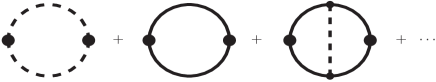
Figure 1: The skeleton expansion of $\Pi_{T}(\tau)$ from (III.3). Dashed and solid lines denote the dressed bosonic and fermionic two-point function $G_{T}(\mathbf{p},\tau)$ from (III.10) and $S_{T}(\mathbf{p},\tau)$ from (III.11), respectively. In our computation up to one-loop skeleton expansion, only the first two diagrams in the above series are considered.

III.1 The bosonic contribution to $\eta$ in the one-loop skeleton expansion

To evaluate the bosonic part of the shear viscosity $\eta_{b}$, we will use the method described in lang2012 , whose main steps will be reviewed in what follows.

Let us first consider (III.8). According to the standard Källen-Lehmann representation, the two-point Green’s function $G_{T}(\mathbf{p},\omega_{n})$ is given in terms of bosonic spectral density function $\rho_{b}(\mathbf{p},\omega)$ as

$$G_{T}({\mathbf{p}},\omega_{n})=\frac{1}{2\pi}\int_{-\infty}^{+\infty}d\omega~{}\frac{\rho_{b}(\mathbf{p},\omega)}{\omega+i\omega_{n}}.$$ (III.12)

Plugging this relation in

$$G_{T}(\mathbf{p},\tau)=\sum_{n=-\infty}^{+\infty}e^{-i\omega_{n}\tau}G_{T}(\mathbf{p},\omega_{n}),$$ (III.13)

and adding over bosonic Matsubara frequencies $\omega_{n}=2n\pi T$, we arrive at

$$G_{T}({\mathbf{p}},\tau)$$ (III.14)

$$=\frac{1}{2\pi}\int_{-\infty}^{+\infty}d\omega~{}e^{-\omega|\tau|}\rho_{b}({\mathbf{p}},\omega)[1+n_{b}(\omega)],$$

where, the bosonic distribution function $n_{b}(\omega)$ reads

$$n_{b}(\omega)\equiv\frac{1}{e^{\beta\omega}-1}.$$ (III.15)

To derive (III.14), we have used the symmetry property $\rho_{b}(\mathbf{p},-\omega)=-\rho_{b}(\mathbf{p},\omega)$, that yields, in particular, $|\tau|$ on the right hand side (r.h.s.) of (III.14). Plugging further $G_{T}(\mathbf{p},\tau)$ from (III.14) in (III.8), and integrating over $\tau$, we arrive after analytical continuation, $i\omega_{n}\to p_{0}+i\epsilon$, at

$$\Pi_{R}^{b}(p_{0})=4\int\frac{d^{3}p}{(2\pi)^{3}}\eta^{\alpha\beta\rho\sigma}p_{\alpha}p_{\beta}p_{\rho}p_{\sigma}$$ (III.16)

$$\times\int_{-\infty}^{+\infty}\frac{d\omega_{1}d\omega_{2}}{(2\pi)^{2}}\rho_{b}({\mathbf{p}},\omega_{1})\rho_{b}({\mathbf{p}},\omega_{2})$$

$$\times~{}n_{b}(\omega_{1})n_{b}(\omega_{2})W_{\epsilon}(\omega_{12},p_{0}),$$

where $\eta^{\alpha\beta\rho\sigma}$ is defined in (III.7), $\omega_{12}\equiv\omega_{1}+\omega_{2}$, and $W_{\epsilon}(\omega_{12},p_{0})$ is given by

$$W_{\epsilon}(\omega_{12},p_{0})\equiv\frac{1}{p_{0}+i\epsilon-\omega_{12}}-\frac{1}{p_{0}+i\epsilon+\omega_{12}}.$$ (III.17)

At this stage, we use the definition of the bosonic spectral density function $\rho_{b}$ in terms of retarded two-point Green’s function, $G_{R}(p)$,

$$\rho_{b}(p)\equiv-2~{}\mathfrak{Im}[G_{R}(p)],$$ (III.18)

to formulate $\rho_{b}$ in terms of the bosonic renormalized energy

$$E_{b}(p)\equiv\sqrt{\omega_{b}^{2}+\mathfrak{Re}[\Sigma_{R}^{b}(p)]},$$ (III.19)

with $\omega_{b}^{2}\equiv\mathbf{p}^{2}+m_{b}^{2}$, and the bosonic spectral width

$$\Gamma_{b}(p)\equiv-\frac{1}{2p_{0}}\mathfrak{Im}[\Sigma_{R}^{b}(p)].$$ (III.20)

Using

$$G_{R}^{-1}(p) = p^{2}-m_{b}^{2}-\Sigma_{R}^{b}(p)$$ (III.21)

$$\simeq [p_{0}+i\Gamma_{b}(p)]^{2}-E_{b}^{2}(p),$$

the bosonic spectral density function (III.18) is given by

$$\rho_{b}(\mathbf{p},\omega)$$

$$= \frac{4\omega\Gamma_{b}(\mathbf{p},\omega_{b})}{[\omega^{2}-E_{b}^{2}(\mathbf{p},\omega_{b})-\Gamma_{b}^{2}(\mathbf{p},\omega_{b})]^{2}+4\omega^{2}\Gamma_{b}^{2}(\mathbf{p},\omega_{b})},$$

where $E_{b}=E_{b}(\mathbf{p},\omega_{b})$ and $\Gamma_{b}=\Gamma_{b}(\mathbf{p},\omega_{b})$ are to be evaluated on mass-shell. Plugging now $\rho_{b}(\mathbf{p},\omega)$ from (III.1) in (III.16), and using lang2012

$$\frac{i}{10}\frac{d}{dp_{0}}W_{\epsilon}(\omega_{12},p_{0})=-\frac{\pi}{5}\delta^{\prime}(\omega_{12}),$$ (III.23)

we arrive first at

$$\eta_{b}=\frac{4\beta}{5\pi}\int\frac{d^{3}p}{(2\pi)^{3}}\eta^{\alpha\beta\rho\sigma}p_{\alpha}p_{\beta}p_{\rho}p_{\sigma}\int_{-\infty}^{+\infty}d\omega F_{b}(\mathbf{p},\omega),$$

with $\omega\equiv\frac{1}{2}\bar{\omega}_{12}\equiv\frac{1}{2}(\omega_{1}-\omega_{2})$ and $F_{b}(\mathbf{p},\omega)$ given by

$$F_{b}(\mathbf{p},\omega)$$

$$= \frac{2\omega^{2}e^{\beta\omega}}{(e^{\beta\omega}-1)^{2}}\frac{\Gamma_{b}^{2}}{[E_{b}^{2}-(\omega-i\Gamma_{b})^{2}]^{2}[E_{b}^{2}-(\omega+i\Gamma_{b})^{2}]^{2}}.$$

Plugging further (III.1) in (III.1) and integrating over $\omega$, using of the same procedure as in lang2012 , and which will be described below, we arrive at the bosonic part of the shear viscosity of the Yukawa theory in terms of the renormalized energy $E_{b}$ from (III.19) and the bosonic spectral width $\Gamma_{b}$ from (III.20),

$$\eta_{b}=\frac{\beta}{30\pi^{2}}\int_{0}^{\infty}dp~{}\frac{\mathbf{p}^{6}}{E_{b}^{2}}~{}\frac{e^{\beta E_{b}}}{\left(e^{\beta E_{b}}-1\right)^{2}}\frac{1}{\Gamma_{b}}+{\cal{O}}(\Gamma_{b}^{0}).$$

To derive (III.1), the pole structure of $F_{b}(\mathbf{p},\omega)$ from (III.1) is to be considered. Following lang2012 , the integral over $\omega$ in (III.1) is to be performed by closing the contour in the upper half-plane, i.e. by considering only two poles $\omega^{\pm}\equiv\pm E_{b}+i\Gamma_{b}$ from four poles $\omega^{\pm}$ and $-\omega^{\pm}$, and eventually expanding the resulting analytical expression in the orders of small $\Gamma_{b}$. This results in

$$2\pi i\sum_{\omega=\omega_{b}^{\pm}}F_{b}(\omega)=\frac{e^{\beta E_{b}}}{(e^{\beta E_{b}}-1)^{2}}\frac{\pi}{16E_{b}^{2}\Gamma_{b}}+{\cal{O}}(\Gamma_{b}^{0}).$$

Let us notice that apart from the aforementioned poles $\omega^{\pm}$ and $-\omega^{\pm}$, there are also an infinite number of poles arising from the denominator $e^{\beta\omega}-1$ in (III.1). But as it is shown in lang2012 , the contributions of their residues are proportional to $\Gamma_{b}^{2}$, and, if we assume that $\Gamma_{b}$ is small enough, they are suppressed relative to the leading $\Gamma_{b}^{-1}$ term in (III.1). Plugging therefore (III.1) in (III.1), and considering the local rest frame of the fluid, we arrive at the bosonic part of the shear viscosity from (III.1). To perform the $p$-integration in (III.1) and study eventually the $T$-dependence of $\eta_{b}$, the $p$ and $T$-dependence of $E_{b}$ and $\Gamma_{b}$ are to be determined perturbatively in an appropriate loop-expansion in the orders of the Yukawa coupling. In this paper, we will approximate $E_{b}\simeq\omega_{b}$ and will determine in Sec. IV only $\Gamma_{b}$ at one-loop level. The result will eventually used to determine the $T$ dependence of $\eta_{b}$. As concerns the $\mu$ dependence of $\eta_{b}$, we will use the same relation (III.1). In this case, the $\mu$ dependence of $\eta_{b}$ arises only from $\Gamma_{b}$ on the r.h.s. of (III.1).

III.2 The fermionic contribution to $\eta$ in the one-loop skeleton expansion

To determine the fermionic part of the shear viscosity $\eta_{f}$, we will follow the same steps as in the previous section, and will present $\eta_{f}$ in terms of fermionic spectral widths $\Gamma_{\pm}$, corresponding to normal and collective excitations of fermions. The resulting expression builds the central analytical result of the present paper.

To start, let us first consider (III.9). Using the standard Källen-Lehmann representation, the fermionic two-point Green’s function $S_{T}(\mathbf{p},\omega_{n})$ can be given in terms of fermionic spectral density function $\rho_{f}(\mathbf{p},\omega)$ as

$$S_{T}({\mathbf{p}},\omega_{n}) = \frac{1}{2\pi}\int_{-\infty}^{+\infty}d\omega~{}\frac{\rho_{f}(\mathbf{p},\omega)}{\omega+i\omega_{n}}.$$ (III.28)

Plugging this relation in

$$S_{T}({\mathbf{p}},\tau)=T\sum_{n=-\infty}^{+\infty}e^{-i\omega_{n}\tau}S_{T}({\mathbf{p}},\omega_{n}),$$ (III.29)

and adding over fermionic Matsubara frequencies $\omega_{n}=(2n+1)\pi T$, we arrive at

$$S_{T}({\mathbf{p}},\tau)=\frac{1}{2\pi}\int_{-\infty}^{+\infty}d\omega~{}e^{-\omega\tau}\rho_{f}({\mathbf{p}},\omega)$$ (III.30)

$$\times\big{[}\theta(\tau)(1-n_{f}(\omega))-\theta(-\tau)n_{f}(\omega)\big{]},$$

with the fermionic distribution function

$$n_{f}(\omega)=\frac{1}{e^{\beta\omega}+1}.$$ (III.31)

Plugging $S_{T}(\mathbf{p},\tau)$ from (III.30) in (III.9), and integrating over $\tau$, using

$$\int_{0}^{\beta}d\tau e^{(i\omega_{n}-\omega_{1}+\omega_{2})\tau}$$

$$\times[\theta(\tau)(1-n_{f}(\omega_{1}))-\theta(-\tau)n_{f}(\omega_{1})]$$

$$\times[\theta(-\tau)(1-n_{f}(\omega_{2}))-\theta(\tau)n_{f}(\omega_{2})]$$

$$=\frac{(1-n_{f}(\omega_{1}))n_{f}(\omega_{2})-(1-n_{f}(-\omega_{1}))n_{f}(-\omega_{2})}{i\omega_{n}-\omega_{1}+\omega_{2}},$$

we arrive first at

$$\Pi_{T}^{f}(\omega_{n})=\frac{1}{2\pi^{2}}\int\frac{d^{3}p}{(2\pi)^{3}}\eta^{\alpha\beta\rho\sigma}p_{\rho}p_{\sigma}$$ (III.33)

$$\times\int d\omega_{1}d\omega_{2}(1-n_{f}(\omega_{1}))n_{f}(\omega_{2})$$

$$\times\bigg{\{}\frac{\mbox{tr}\left(\rho_{f}(\omega_{1},\mathbf{p})\gamma_{\alpha}\rho_{f}(\omega_{2},\mathbf{p})\gamma_{\beta}\right)}{i\omega_{n}-\omega_{1}+\omega_{2}}$$

$$-\frac{\mbox{tr}\left(\rho_{f}(-\omega_{1},-\mathbf{p})\gamma_{\alpha}\rho_{f}(-\omega_{2},-\mathbf{p})\gamma_{\beta}\right)}{i\omega_{n}+\omega_{1}-\omega_{2}}\bigg{\}},$$

where $\eta^{\alpha\beta\rho\sigma}$ is defined below (III.6). To evaluate $\Pi_{T}(\omega_{n})$, let us use at this stage, in analogy to the bosonic case, the definition of the fermionic spectral density function $\rho_{f}$ in term of the retarded two-point Green’s function $S_{R}$,

$$\rho_{f}(p)=-2~{}\mathfrak{Im}[S_{R}(p)],$$ (III.34)

and the decomposition of $S_{R}(p)$ in term the fermion self-energy $\Sigma_{R}^{f}$,

$$S_{R}^{-1}(p)=\gamma\cdot p-m_{f}+\Sigma_{R}^{f}(p).$$ (III.35)

Using the method, described in details in App. A, the spectral density function of fermions is given by

$$\rho_{f}(\mathbf{p},\omega)=\frac{2\Gamma_{+}(\mathbf{p},\omega_{f})}{[\omega-E_{+}(\mathbf{p},\omega_{f}]^{2}+\Gamma_{+}^{2}(\mathbf{p},\omega_{f})}\hat{g}_{+}(\mathbf{p},\omega_{f})$$ (III.36)

$$-\frac{2\Gamma_{-}(\mathbf{p},\omega_{f})}{[\omega+E_{-}(\mathbf{p},\omega_{f})]^{2}+\Gamma_{-}^{2}(\mathbf{p},\omega_{f})}\hat{g}_{-}(\mathbf{p},\omega_{f}),$$

where $\omega_{f}^{2}=\mathbf{p}^{2}+m_{f}^{2}$, and

$$\hat{g}_{\pm}(\mathbf{p},\omega_{f})=\frac{1}{2\omega_{f}}\big{[}\gamma_{0}\omega_{f}\mp\left(\gamma.\mathbf{p}-m_{f}\right)\big{]}.$$ (III.37)

In (III.36), $E_{\pm}$ and $\Gamma_{\pm}$ are defined by [see App. A for more details]

$$E_{\pm}(\mathbf{p},\omega_{f}) \equiv \omega_{f}\pm\frac{1}{2}\mbox{tr}\left(\hat{g}_{\pm}(\mathbf{p},\omega_{f})\mathfrak{Re}[\Sigma_{R}^{f}(\mathbf{p},\omega_{f})]\right),$$

$$\Gamma_{\pm}(\mathbf{p},\omega_{f}) \equiv \pm\frac{1}{2}\mbox{tr}\left(\hat{g}_{\pm}(\mathbf{p},\omega_{f})\mathfrak{Im}[\Sigma_{R}^{f}(\mathbf{p},\omega_{f})]\right).$$

In jeon2007 , almost the same expression for $\rho_{f}$ as in (III.36) is introduced. However, in contrast to (III.36), only one spectral width for the fermion appears in the relation presented in jeon2007 . Apparently, $\Gamma_{+}\simeq\Gamma_{-}$ is assumed. In what follows, we do not make this approximation, and after deriving $\eta_{f}$ in terms of $\Gamma_{\pm}$, we will explore the effect of $\Gamma_{+}$ and $\Gamma_{-}$ on the thermal properties of $\eta_{f}$. Let us notice at this stage, that the plus and minus signs appearing on $E_{\pm}$ and $\Gamma_{\pm}$ correspond to the normal and collective (plasmino) modes of the fermions weldon1989 . In the chiral limit $m_{f}\to 0$, they correspond to the same and opposite helicity and chirality of massless fermions, respectively weldon1999 .

Let us now consider (III.33), which will be simplified in what follows. Using the symmetry properties of $E_{\pm}(p)$ and $\Gamma_{\pm}(p)$,

$$E_{\pm}(\mathbf{p},-\omega_{f}) = -E_{\pm}(\mathbf{p},\omega_{f}),$$

$$\Gamma_{\pm}(\mathbf{p},-\omega_{f}) = +\Gamma_{\pm}(\mathbf{p},\omega_{f}),$$ (III.39)

which we could verify only at one-loop level, we obtain

$$\rho_{f}(-\mathbf{p},-\omega)=\rho_{f}(\mathbf{p},\omega)$$ (III.40)

$$-\frac{2m_{f}}{\omega_{f}}\bigg{\{}\frac{\Gamma_{+}(\mathbf{p},\omega_{f})}{[\omega-E_{+}(\mathbf{p},\omega_{f})]^{2}+\Gamma_{+}^{2}(\mathbf{p},\omega_{f})}$$

$$+\frac{\Gamma_{-}(\mathbf{p},\omega_{f})}{[\omega+E_{-}(\mathbf{p},\omega_{f})]^{2}+\Gamma_{-}^{2}(\mathbf{p},\omega_{f})}\bigg{\}}.$$

Using (III.40) together with the properties of the traces of Dirac $\gamma$-matrices, we have

$$\mbox{tr}\left(\rho_{f}(-\mathbf{p},-\omega_{1})\gamma_{\alpha}\rho_{f}(-\mathbf{p},-\omega_{2})\gamma_{\beta}\right)$$ (III.41)

$$=\mbox{tr}\left(\rho_{f}(\mathbf{p},\omega_{1})\gamma_{\alpha}\rho_{f}(\mathbf{p},\omega_{2})\gamma_{\beta}\right).$$

Implementing now this relation in (III.33), we arrive after analytical continuation, $i\omega_{n}\to p_{0}+i\epsilon$, at

$$\Pi_{R}^{f}(p_{0})=\frac{1}{2\pi^{2}}\int\frac{d^{3}p}{(2\pi)^{3}}\eta^{\alpha\beta\rho\sigma}p_{\rho}p_{\sigma}$$ (III.42)

$$\times\int_{-\infty}^{+\infty}d\omega_{1}d\omega_{2}\mbox{tr}\left(\rho_{f}(\omega_{1},\mathbf{p})\gamma_{\alpha}\rho_{f}(\omega_{2},\mathbf{p})\gamma_{\beta}\right)$$

$$\times~{}(1-n_{f}(\omega_{1}))n_{f}(\omega_{2})W_{\epsilon}(\bar{\omega}_{12},p_{0}),$$

where $\bar{\omega}_{12}\equiv\omega_{1}-\omega_{2}$ and $W_{\epsilon}$ is defined in (III.17). To derive the fermionic part of the shear viscosity $\eta_{f}$ from (II.15), we follow the same steps as is presented in the previous section for the bosonic case. Plugging (III.36) in (III.42), and after performing a straightforward mathematical computation, where mainly the relations

$$\frac{i}{10}\frac{d}{dp_{0}}W_{\epsilon}(p_{0},\bar{\omega}_{12})\bigg{|}_{p_{0}=0}=-\frac{\pi}{5}\delta^{\prime}(\bar{\omega}_{12}),$$ (III.43)

and

$$\mbox{tr}\left(\hat{g}_{\pm}\gamma_{\alpha}\hat{g}_{\mp}\gamma_{\rho}\right)$$

$$= \frac{1}{\omega_{f}^{2}}\bigg{\{}2\omega_{f}^{2}(g_{0\alpha}g_{0\rho}-g_{\alpha\rho})-p_{i}p_{j}(g_{\alpha}^{i}g_{\rho}^{j}+g_{\rho}^{i}g_{\alpha}^{j})\bigg{\}}.$$

$$\mbox{tr}\left(\hat{g}_{\pm}\gamma_{\alpha}\hat{g}_{\pm}\gamma_{\rho}\right)=\frac{1}{\omega_{f}^{2}}\bigg{\{}2\omega_{f}^{2}g_{0\alpha}g_{0\rho}\mp 2\omega_{f}p_{i}(g_{\alpha}^{0}g_{\rho}^{i}$$ (III.44)

$$+g_{\rho}^{0}g_{\alpha}^{i})+p_{i}p_{j}(g_{\alpha}^{i}g_{\rho}^{j}+g_{\rho}^{i}g_{\alpha}^{j})\bigg{\}},$$

in the local rest frame of the fluid are used, we arrive at

$$\eta_{f}=\frac{8\beta}{15\pi}\int\frac{d^{3}p}{(2\pi)^{3}}\int_{-\infty}^{+\infty}d\omega~{}F_{f}(\mathbf{p},\omega),$$ (III.45)

with

$$F_{f}(\mathbf{p},\omega)\equiv\frac{e^{\beta\omega}}{(e^{\beta\omega}+1)^{2}}\mathbf{p}^{2}$$ (III.46)

$$\times\bigg{\{}\frac{\mathbf{p}^{2}}{\omega_{f}^{2}}\left(\frac{\Gamma_{+}}{(\omega-E_{+})^{2}+\Gamma_{+}^{2}}+\frac{\Gamma_{-}}{(\omega+E_{-})^{2}+\Gamma_{-}^{2}}\right)^{2}$$

$$-\frac{2~{}\Gamma_{+}\Gamma_{-}}{[(\omega-E_{+})^{2}+\Gamma_{+}^{2}][(\omega+E_{-})^{2}+\Gamma_{-}^{2}]}\bigg{\}},$$

where $\omega\equiv\frac{1}{2}\omega_{12}=\frac{1}{2}(\omega_{1}-\omega_{2})$, and $E_{\pm}=E_{\pm}(\mathbf{p},\omega_{f})$ as well as $\Gamma_{\pm}=\Gamma_{\pm}(\mathbf{p},\omega_{f})$ are defined in (III.2). To evaluate the integration over $\omega$ in (III.46), the pole structure of $F_{f}(\mathbf{p},\omega)$ is to be considered. Similar to the previous case of bosonic fields, the contributions of the poles arising from the denominator $e^{\beta\omega}+1$ in (III.46) turn out to be proportional to $\Gamma_{\pm}^{2}$, and, assuming that $\Gamma_{+}$ and $\Gamma_{-}$ are small enough, they can be neglected. As concerns the residue of the remaining poles, we have to close the contour in the upper half-plane and consider only two residue $\omega^{\pm}\equiv\pm E_{\pm}+i\Gamma_{\pm}$. Expanding the resulting expression in the orders of $\Gamma_{\pm}$ in a Laurent series in the orders of $\Gamma_{\pm}$, and using

$$\int_{-\infty}^{+\infty}d\omega\frac{e^{\beta\omega}}{(e^{\beta\omega}+1)^{2}}\frac{\Gamma_{\pm}^{2}}{[(\omega\mp E_{\pm})^{2}+\Gamma^{2}_{\pm}]^{2}}$$

$$\approx\pi\frac{e^{\beta E_{\pm}}}{(e^{\beta E_{\pm}}+1)^{2}}\frac{1}{2\Gamma_{\pm}},$$

$$\int_{-\infty}^{+\infty}d\omega\frac{\Gamma_{+}\Gamma_{-}}{[(\omega-E_{+})^{2}+\Gamma_{+}^{2}][(\omega+E_{-})^{2}+\Gamma_{-}^{2}]}$$

$$\approx\pi\sum_{s=\pm}\frac{e^{\beta E_{s}}}{(e^{\beta E_{s}}+1)^{2}}\frac{\Gamma_{f}^{+}-\Gamma_{s}}{[E_{f}+is~{}\Gamma_{f}^{+}][E_{f}+i\Gamma_{f}^{-}]},$$

where

$$E_{f}\equiv E_{+}+E_{-},\qquad\Gamma_{f}^{\pm}\equiv\Gamma_{+}\pm\Gamma_{-},$$ (III.48)

we arrive, after performing the integration over three-dimensional angles in (III.45), at the fermionic part of the shear viscosity of the Yukawa theory,

$$\eta_{f}=\frac{2\beta}{15\pi^{2}}\int_{0}^{\infty}dp\frac{\mathbf{p}^{4}}{\omega_{f}^{2}}\sum_{s=\pm}\bigg{\{}\frac{e^{\beta E_{s}}}{(e^{\beta E_{s}}+1)^{2}}$$

$$\times\bigg{[}\frac{\mathbf{p}^{2}}{\Gamma_{s}}-\frac{4m_{f}^{2}(\Gamma_{f}^{+}-\Gamma_{s})}{[E_{f}+is\Gamma_{f}^{+}][E_{f}+i\Gamma_{f}^{-}]}\bigg{]}\bigg{\}}+{\cal{O}}(\Gamma_{\pm}^{0}).$$

Here, $E_{f}=E_{f}(\mathbf{p},\omega_{f})$, $\Gamma_{\pm}=\Gamma_{\pm}(\mathbf{p},\omega_{f})$ and $\Gamma_{f}^{\pm}=\Gamma_{f}^{\pm}(\mathbf{p},\omega_{f})$ are defined in (III.2) and (III.48). Let us notice that the first term of above relation for $\eta_{f}$ is comparable with the shear viscosity corresponding to fermions appearing in ghosh2013 in a relaxation time approximation. Moreover, it resembles the $\eta_{f}$ presented recently in lang2013 . Here, the authors express $\eta_{f}$ first in terms of fermionic density function, $\rho_{f}$, which in contrast to (III.36), possesses a generalized Breit-Wigner shape, including only a quasiparticle mass $M$ and a fermionic width $\Gamma_{f}$. Using this Ansatz for $\rho_{f}$, they arrive then at $\eta_{f}$ in this quasiparticle approximation (see Eq. (22) in lang2013 ). We, however, will work with (III.2) and after determining $\Gamma_{\pm}$ in a one-loop perturbative expansion, in the next section, will study the thermal properties of $\eta_{f}[\Gamma_{\pm}]$ for various masses $m_{b}$ and $m_{f}$. We will then determine the difference between $\eta_{f}[\Gamma_{+}=\Gamma_{-}]$ and $\eta_{f}[\Gamma_{+}\neq\Gamma_{-}]$. In App. C, we will generalize the method presented in this section for the case of non-vanishing chemical potential. We will show that in this case (C.1), replaces (III.2), and can be used to explore the thermal properties of $\eta_{f}$ at finite $T$ and $\mu$.

IV Perturbative computation of bosonic and fermionic spectral widths

In this section, we will perturbatively compute the bosonic and fermionic spectral widths of the Yukawa theory from (III.20) and (III.2) at one-loop level. To do this, the imaginary part of the one-loop bosonic and fermionic self-energy diagrams will be evaluated using the standard Schwinger-Keldysh real-time formalism schwinger1961 . In what follows, we will closely follow the notations of dasbook and kobes1985 . According to this formalism, the free propagator of scalar bosons is given by

$${\cal{G}}=\left(\begin{array}[]{cc}G_{++}&G_{+-}\\ G_{-+}&G_{--}\end{array}\right),$$ (IV.3)

where $G_{ab},a,b=\pm$ read

$$G_{++}(p) = -\frac{i}{p^{2}-m_{b}^{2}+i\epsilon}-2\pi n_{b}(|p_{0}|)\delta(p^{2}-m_{b}^{2}).$$

$$G_{+-}(p) = -2\pi[\theta(-p_{0})+n_{b}(|p_{0}|)]\delta(p^{2}-m_{b}^{2}),$$

$$G_{-+}(p) = -2\pi[\theta(p_{0})+n_{b}(|p_{0}|)]\delta(p^{2}-m_{b}^{2}),$$

$$G_{--}(p) = \frac{i}{p^{2}-m_{b}^{2}-i\epsilon}-2\pi n_{b}(|p_{0}|)\delta(p^{2}-m_{b}^{2}).$$

Here, $m_{b}$ is the boson mass and $n_{b}(p_{0})$ the bosonic distribution function defined in (III.15). Similarly, the free fermion propagator is given by

$${\cal{S}}=\left(\begin{array}[]{cc}S_{++}&S_{+-}\\ S_{-+}&S_{--}\end{array}\right),$$ (IV.7)

with the components

$$S_{++}(p) = (\gamma\cdot p+m_{f})\left(-\frac{i}{p^{2}-m_{f}^{2}+i\epsilon}+2\pi n_{f}(|p_{0}|)\delta(p^{2}-m_{f}^{2})\right),$$

$$S_{+-}(p) = -2\pi(\gamma\cdot p+m_{f})[\theta(-p_{0})-n_{f}(|p_{0}|)]\delta(p^{2}-m_{f}^{2}),$$

$$S_{-+}(p) = -2\pi(\gamma\cdot p+m_{f})[\theta(p_{0})-n_{f}(|p_{0}|)]\delta(p^{2}-m_{f}^{2}),$$

$$S_{--}(p) = (\gamma\cdot p+m_{f})\left(\frac{i}{p^{2}-m^{2}-i\epsilon}+2\pi n_{f}(|p_{0}|)\delta(p^{2}-m_{f}^{2})\right).$$ (IV.8)

Here, $m_{f}$ is the fermion mass and $n_{f}(p_{0})$ the fermionic distribution function defined in (III.31). Combining $G_{ab},a,b=\pm$ and $S_{ab},a,b=\pm$, the physical retarded (R) and advanced (A) two-point Green’s functions for scalar bosons, $G_{R/A}$, and fermions, $S_{R/A}$, are given by

$$G_{R}=G_{++}+G_{+-},\qquad G_{A}=G_{++}+G_{-+},$$ (IV.9)

and

$$S_{R}=S_{++}+S_{+-},\qquad\hskip 5.69046ptS_{A}=S_{++}+S_{-+}.$$ (IV.10)

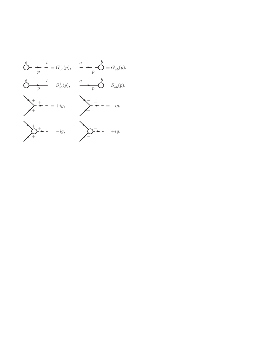
Figure 2: Feynman rules, that are necessary to compute the imaginary part of bosonic and fermionic one-loop self-energy diagrams of the Yukawa theory (see Figs. 3 and 4). The definitions of $G_{ab}^{\pm}$ and $S_{ab}^{\pm}$ with $a,b=\pm$ in terms of $G_{ab}$ and $S_{ab}$ from (IV) and (IV) are presented in (IV).

To determine the spectral widths, $\Gamma_{b}$ and $\Gamma_{\pm}$ from (III.20) and (III.2), the imaginary parts of the bosonic and fermionic one-loop self-energies, $\Sigma_{R}^{b}$ and $\Sigma_{R}^{f}$, are to be computed. In the real-time formalism, this is done using the finite temperature cutting rules dasbook ; kobes1985 . The main ingredients of these rules are specific propagators and vertices, that for the Yukawa theory, are demonstrated in Fig. 2.

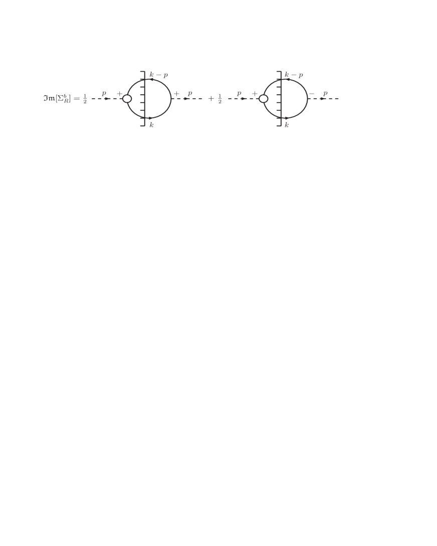
Figure 3: Diagrammatic representation of the cutting rules leading to the imaginary part of the retarded part of the one-loop self-energy diagram for scalar bosons, $\Sigma_{R}^{b}$ in the Yukawa theory.

Here, $G_{ab}^{\pm}$ and $S_{ab}^{\pm}$ with $a,b=\pm$ are the retarded ($+$) and advanced ($-$) part of the bosonic and fermionic Green’s functions. They are defined in the following decomposition for a generic Green’s function, ${\cal{D}}_{ab}$, with $a,b=\pm$,

$${\cal{D}}_{ab}(x)=\theta(t){\cal{D}}_{ab}^{+}(x)+\theta(-t){\cal{D}}_{ab}^{-}(x).$$ (IV.11)

Using the definitions ${\cal{D}}_{ab},a,b=\pm$ and ${\cal{D}}=\{G,S\}$, from (IV) and (IV), we get the following identities:

$${\cal{D}}_{++}^{+}={\cal{D}}_{--}^{-}={\cal{D}}_{-+}^{+}={\cal{D}}_{-+}^{-}={\cal{D}}_{-+},$$

$${\cal{D}}_{++}^{-}={\cal{D}}_{--}^{+}={\cal{D}}_{+-}^{+}={\cal{D}}_{+-}^{-}={\cal{D}}_{+-}.$$ (IV.12)

In what follows, we will separately compute the imaginary part of the one-loop self-energy corrections to bosonic and fermionic two-point Green’s functions. The results will eventually be used to determine the bosonic and fermionic spectral widths.

IV.1 Bosonic spectral width in one-loop perturbative expansion

Let us consider the bosonic spectral width $\Gamma_{b}$ from (III.20), that evaluated at $\omega_{b}=(\mathbf{p}^{2}+m_{b}^{2})^{1/2}$ reads

$$\Gamma_{b}(\mathbf{p},\omega_{b})=-\frac{1}{2\omega_{b}}\mathfrak{Im}[\Sigma_{R}^{b}(\mathbf{p},\omega_{b})].$$ (IV.13)

To determine the imaginary part of $\Sigma_{R}^{b}(p)$ at one-loop level, we will use the diagrammatic representation of the cutting rules dasbook ; kobes1985 , demonstrated in Fig. 3. Using the propagators and vertices presented in Fig. 2, the imaginary part of $\Sigma_{R}^{b}(p)$ reads

$$\mathfrak{Im}[\Sigma_{R}^{b}(p)] = -\frac{g^{2}}{2}\int\frac{d^{4}k}{(2\pi)^{4}}\mbox{tr}\left(S_{++}^{-}(k-p)S_{++}^{+}(k)\right.$$ (IV.14)

$$\left.-S_{-+}^{-}(k-p)S_{+-}^{+}(k)\right),$$

where, according to (IV.11) with ${\cal{D}}_{ab}=S_{ab}$, $S_{ab}^{+}$ and $S_{ab}^{-}$ are the retarded and advanced parts of the fermionic Green’s function $S_{ab},a,b=\pm$ from (IV), respectively. To derive the spectral width of bosons, we use the identities (IV) together with (IV), and arrive after performing the integration over $k_{0}$ and some straightforward manipulations first at

$$\Gamma_{b}(\mathbf{p},\omega_{b})=\frac{g^{2}}{8\omega_{b}}\int\frac{d^{3}k}{(2\pi)^{2}}\frac{(4m_{f}^{2}-m_{b}^{2})}{\omega_{1}\omega_{2}}$$

$$\times\bigg{\{}\delta(\omega_{b}-\omega_{1}-\omega_{2})[1-n_{f}(\omega_{1})-n_{f}(\omega_{2})]$$

$$~{}~{}+\delta(\omega_{b}-\omega_{1}+\omega_{2})[n_{f}(\omega_{1})-n_{f}(\omega_{2})]$$

$$~{}~{}-\delta(\omega_{b}+\omega_{1}-\omega_{2})[n_{f}(\omega_{1})-n_{f}(\omega_{2})]$$

$$~{}~{}-\delta(\omega_{b}+\omega_{1}+\omega_{2})[1-n_{f}(\omega_{1})-n_{f}(\omega_{2})]\bigg{\}}.$$

Here, $\omega_{1}^{2}\equiv\mathbf{k}^{2}+m_{f}^{2}$ and $\omega_{2}^{2}\equiv(\mathbf{k}-\mathbf{p})^{2}+m_{f}^{2}$. The factor $(4m_{f}^{2}-m_{b}^{2})$ on the r.h.s. of (IV.1) arises by considering the on mass-shell relations, $k^{2}=m_{f}^{2}$ and $(k-p)^{2}=m_{f}^{2}$ from the Dirac-$\delta$-functions, appearing in $S_{ab}$ from (IV.14), with $S_{ab},a,b=\pm$ given in (IV). Using now the definition of the fermionic distribution functions $n_{f}(\omega)$ from (III.31), we get

$$\Gamma_{b}(\mathbf{p},\omega_{b})=\frac{g^{2}}{16\omega_{b}}\int\frac{d^{3}k}{(2\pi)^{2}}\frac{\sinh(\frac{\beta\omega_{b}}{2})}{\cosh(\frac{\beta\omega_{1}}{2})\cosh(\frac{\beta\omega_{2}}{2})}$$ (IV.16)

$$\times\frac{(4m_{f}^{2}-m_{b}^{2})}{\omega_{1}\omega_{2}}\bigg{\{}\delta(\omega_{b}-\omega_{1}-\omega_{2})-\delta(\omega_{b}-\omega_{1}+\omega_{2})$$

$$\qquad-\delta(\omega_{b}+\omega_{1}-\omega_{2})+\delta(\omega_{b}+\omega_{1}+\omega_{2})\bigg{\}}.$$

Note that in the rest-frame of the scalar bosons with $\mathbf{p}=0$, only the first term on the r.h.s. of (IV.1), proportional to $\delta(\omega_{b}-\omega_{1}-\omega_{2})$ will contribute. It leads to $m_{b}\geq 2m_{f}$, as a constraint on the relation between bosonic and fermionic masses. Thus, keeping in mind that $\Gamma_{b}(\mathbf{p},\omega_{b})$ is Lorentz invariant, it is in general given by

$$\Gamma_{b}(\mathbf{p},\omega_{b}) = \frac{g^{2}}{16\omega_{b}}\int\frac{d^{3}k}{(2\pi)^{2}}\frac{\sinh(\frac{\beta\omega_{b}}{2})}{\cosh(\frac{\beta\omega_{1}}{2})\cosh(\frac{\beta\omega_{2}}{2})}$$ (IV.17)

$$\times\frac{(4m_{f}^{2}-m_{b}^{2})}{\omega_{1}\omega_{2}}\delta(\omega_{b}-\omega_{1}-\omega_{2}).$$

After performing the integration over $k$, using the method described in App. C, the bosonic part of the spectral width of the Yukawa theory, evaluated in a one-loop perturbative expansion, reads

$$\Gamma_{b}(\mathbf{p},\omega_{b})=\frac{g^{2}T}{16\pi}\frac{\gamma_{b}^{2}(\xi^{2}-4)}{\xi^{2}\sqrt{1-\gamma_{b}^{2}}}$$ (IV.18)

$$\times\ln\bigg{[}\frac{1+\cosh\frac{\kappa_{b}}{2}(1+\frac{1}{\xi}\sqrt{(\xi^{2}-4)(1-\gamma_{b}^{2})})}{1+\cosh\frac{\kappa_{b}}{2}(1-\frac{1}{\xi}\sqrt{(\xi^{2}-4)(1-\gamma_{b}^{2})})}\bigg{]}.$$

Here, $\xi\equiv\frac{m_{b}}{m_{f}}$ and $\gamma_{b}\equiv\frac{m_{b}}{\omega_{b}}$, with $\omega_{b}^{2}=\mathbf{p}^{2}+m_{b}^{2}$. Moreover, $\kappa_{b}\equiv\omega_{b}/T$. In App. C, we have generalized the result presented in (IV.18) to the case of non-vanishing chemical potential, $\mu$. In this case, the one-loop contribution to the bosonic spectral width is presented in (C.16). In Sec. V, we will use (IV.18) and (C.16) to study the the thermal properties of $\Gamma_{b}$. Eventually $\Gamma_{b}$ will be inserted in (III.1) and the thermal properties of $\eta_{b}$ for various $\xi$ will be studied.

IV.2 Fermionic spectral width in one-loop perturbative expansion

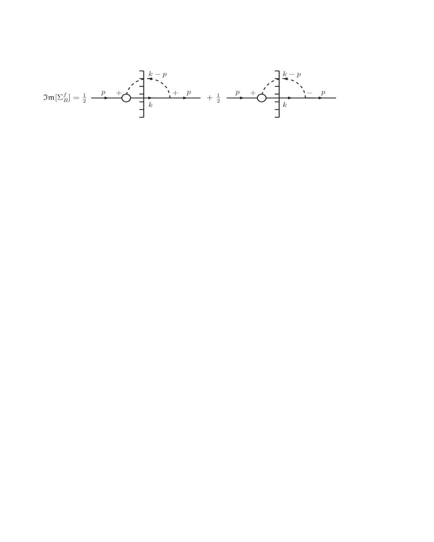
Figure 4: Diagrammatic representation of the cutting rules leading to the imaginary part of the retarded part of the one-loop self-energy diagram for fermions, $\Sigma_{R}^{f}$ in the Yukawa theory.

As we have demonstrated in the previous section, fermions possess two different spectral widths $\Gamma_{\pm}$, defined in (III.2). They can be perturbatively computed by evaluating the imaginary part of the retarded fermion self-energy $\Sigma_{R}^{f}$ in an appropriate loop expansion. In what follows, in analogy to the bosonic case, the standard finite temperature cutting rules from dasbook ; kobes1985 will be used to evaluate the imaginary part of $\Sigma_{R}^{f}$ at one-loop level. Using the Feynman rules presented in Fig. 2, and the diagrammatic representation of $\mathfrak{Im}[\Sigma_{R}^{f}]$ demonstrated in Fig. 4, we arrive first at

$$\mathfrak{Im}[\Sigma_{R}^{f}(p)] = \frac{g^{2}}{2}\int\frac{d^{4}k}{(2\pi)^{4}}\big{[}S_{++}^{+}(k)G_{++}^{-}(k-p)$$ (IV.19)

$$-S_{+-}^{+}(k)G_{-+}^{-}(k-p)\big{]},$$

where ${\cal{D}}_{ab}^{\pm},a,b=\pm$ and ${\cal{D}}_{ab}=\{G,S\}$ are defined in (IV.11). Using the identities (IV), with ${\cal{D}}=\{G,S\}$, together with the definitions of $G_{ab}$ and $S_{ab},a,b=\pm$ from (IV) and (IV), we arrive after performing the integration over $k_{0}$ in (IV.19) and some straightforward manipulations, at the fermionic spectral widths $\Gamma_{\pm}$, defined originally in (III.2),

$$\Gamma_{\pm}(\mathbf{p},\omega_{f})=\pm\frac{g^{2}}{8\omega_{f}}\int\frac{d^{3}k}{(2\pi)^{2}}\frac{1}{\omega_{1}\omega_{2}}$$ (IV.20)

$$\times\bigg{[}[\omega_{f}\omega_{1}\mp\mathbf{p}\cdot\mathbf{k}\pm m_{f}^{2}]\big{\{}\delta(\omega_{f}-\omega_{1}-\omega_{2})[1-n_{f}(\omega_{1})+n_{b}(\omega_{2})]+\delta(\omega_{f}-\omega_{1}+\omega_{2})[n_{f}(\omega_{1})+n_{b}(\omega_{2})]\big{\}}$$

$$+[\omega_{f}\omega_{1}\pm\mathbf{p}\cdot\mathbf{k}\mp m_{f}^{2}]\big{\{}\delta(\omega_{f}+\omega_{1}+\omega_{2})[1-n_{f}(\omega_{1})+n_{b}(\omega_{2})]+\delta(\omega_{f}+\omega_{1}-\omega_{2})[n_{f}(\omega_{1})+n_{b}(\omega_{2})]\big{\}}\bigg{]}.$$

According to our notations from Fig. 4, $\omega_{f}^{2}\equiv{\mathbf{p}}^{2}+m_{f}^{2}$ corresponds to the momentum of the external fermion propagators, and $\omega_{1}^{2}\equiv k_{0}^{2}=\mathbf{k}^{2}+m_{f}^{2}$ and $\omega_{2}^{2}\equiv(k_{0}-p_{0})^{2}=(\mathbf{k}-\mathbf{p})^{2}+m_{b}^{2}$ to the internal fermion and boson propagators, respectively. Here, in contrast to the bosonic case, only two terms on the r.h.s. of (IV.20), proportional to $\delta(\omega_{f}-\omega_{1}+\omega_{2})$ and $\delta(\omega_{f}+\omega_{1}-\omega_{2})$, contribute to the final results of $\Gamma_{+}$ and $\Gamma_{-}$. This is because of the specific kinematics of $f\to bf$ process in the rest frame of the particles. Here, $b$ and $f$ correspond to boson and fermion, respectively. Thus, the fermionic spectral widths are determined after some algebraic manipulations, where the definitions (III.15) and (III.31) of bosonic and fermionic distribution functions are used. For $\Gamma_{+}$, we obtain

$$\Gamma_{+}(\mathbf{p},\omega_{f})$$ (IV.21)

$$=\frac{g^{2}}{32\omega_{f}}\int\frac{d^{3}k}{(2\pi)^{2}}\frac{(4m_{f}^{2}-m_{b}^{2})}{\omega_{1}\omega_{2}}\frac{\cosh(\frac{\beta\omega_{f}}{2})}{\cosh(\frac{\beta\omega_{1}}{2})\sinh(\frac{\beta\omega_{2}}{2})}$$

$$~{}\times\bigg{\{}\delta(\omega_{f}-\omega_{1}+\omega_{2})-\delta(\omega_{f}+\omega_{1}-\omega_{2})\bigg{\}}.$$

As concerns $\Gamma_{-}$, it is given, according to (III.48), by $\Gamma_{-}=\Gamma_{+}-\Gamma_{f}^{-}$, where $\Gamma_{f}^{-}$ is given by

$$\Gamma_{f}^{-}(\mathbf{p},\omega_{f})=\frac{g^{2}}{8}\int\frac{d^{3}k}{(2\pi)^{2}\omega_{2}}\frac{\cosh(\frac{\beta\omega_{f}}{2})}{\cosh(\frac{\beta\omega_{1}}{2})\sinh(\frac{\beta\omega_{2}}{2})}$$ (IV.22)

$$\times\bigg{\{}\delta(\omega_{f}-\omega_{1}+\omega_{2})+\delta(\omega_{f}+\omega_{1}-\omega_{2})\bigg{\}}.$$

Performing the integration over $k$ in (IV.21), by making use of the method presented in App. B, $\Gamma_{+}$ reads

$$\Gamma_{+}(\xi,\gamma_{f},\kappa_{f};T)=\frac{g^{2}T}{32\pi}\frac{\gamma_{f}^{2}(\xi^{2}-4)}{\sqrt{1-\gamma_{f}^{2}}}$$

$$\times\bigg{\{}\ln\bigg{[}\frac{1-\cosh(2~{}\Xi_{-})}{\cosh(\Upsilon_{-}+\Xi_{+})-\cosh(\Upsilon_{-}-\Xi_{+})}\bigg{]}$$

$$-\ln\bigg{[}\frac{1+\cosh(2~{}\Xi_{-}-\kappa_{f})}{\cosh(\Upsilon_{-}+\Xi_{+})+\cosh(\Upsilon_{+}-\Xi_{+})}\bigg{]}\bigg{\}}.$$

Here, $\xi=\frac{m_{b}}{m_{f}}$ and $\gamma_{f}\equiv\frac{m_{f}}{\omega_{f}}$ with $\omega_{f}^{2}=\mathbf{p}^{2}+m_{f}^{2}$. Moreover, we have

$$\Xi_{\pm} = \frac{\kappa_{f}}{4}\xi[\xi\pm\sqrt{(\xi^{2}-4)(1-\gamma_{f}^{2})}],$$

$$\Upsilon_{\pm} = \frac{\kappa_{f}}{2}(\gamma_{f}\pm 1),$$ (IV.24)

with $\kappa_{f}\equiv\omega_{f}/T$. Similarly, the integration over $k$ in (IV.22) can be performed analytically. This is done in App. B, where the final result for $\Gamma_{f}^{-}$ is presented in (B). In App. C, the same method is used for the case of non-vanishing chemical potential and $\Gamma_{+}$ and $\Gamma_{f}^{-}$ are determined at one-loop level. The results for $\Gamma_{+}$ and $\Gamma_{f}^{-}$ are presented in (C.2) and (C.2), respectively.

In Sec. V, we will study the qualitative behavior of dimensionless quantities $\Gamma_{+}/g^{2}T$ and $\Gamma_{f}^{-}/g^{2}T$ in terms of dimensionless variables $\xi,\gamma_{f}$ and $\kappa_{f}$. We will then study the $T$ and $\mu$ dependence of $\Gamma_{+}$ and $\Gamma_{-}$, and will show that in certain regime of parameter space $\Gamma_{f}^{-}=\Gamma_{+}-\Gamma_{-}$ is not negligible. Plugging the resulting expressions for $\Gamma_{\pm}$ and $\Gamma_{f}^{-}$ in (III.2) and assuming that $E_{f}\sim\omega_{f}=(\mathbf{p}^{2}+m_{f}^{2})^{1/2}$, we will eventually explore the thermal properties of the fermionic part of the shear viscosity.

V Numerical Results

In this section, we will mainly study the $T$ and $\mu$ dependence of bosonic and fermionic spectral widths $\Gamma_{b}$ and $\Gamma_{\pm}$, as well as the thermal properties of bosonic and fermionic part of the shear viscosity, $\eta_{b}$ and $\eta_{f}$. We will first determine the $T$ and $\mu$ dependence of these quantities for constant $\xi_{0}\equiv m_{b}^{0}/m_{f}^{0}$, including the $T$ and $\mu$ independent bosonic and fermionic masses, $m_{b}^{0}$ and $m_{f}^{0}$, respectively. We then consider the standard thermal corrections of bosonic and fermionic masses kiessig2010 , arising from standard HTL approximation,

$$(m_{b}^{\mbox{\tiny{th}}})^{2} = \frac{g^{2}}{6}\left(T^{2}+\frac{3\mu^{2}}{\pi^{2}}\right),$$

$$(m_{f}^{\mbox{\tiny{th}}})^{2} = \frac{g^{2}}{16}\left(T^{2}+\frac{\mu^{2}}{\pi^{2}}\right),$$ (V.1)

and will add these thermal corrections to the original constant $m_{b}^{0}$ and $m_{f}^{0}$. Using the definition

$$\xi(T,\mu)\equiv\frac{m_{b}(T,\mu)}{m_{f}(T,\mu)},$$ (V.2)

with

$$m_{b}(T,\mu) \equiv m_{b}^{0}+m_{b}^{\mbox{\tiny{th}}}(T,\mu),$$

$$m_{f}(T,\mu) \equiv m_{f}^{0}+m_{f}^{\mbox{\tiny{th}}}(T,\mu),$$ (V.3)

we will then determine the $T$ and $\mu$ dependence of $\Gamma_{b},\Gamma_{\pm}$ as well as $\eta_{b}$ and $\eta_{f}$, including the thermal corrections to bosonic and fermionic masses. According to the descriptions in kiessig2009 ; kiessig2010 , and since in the Yukawa theory the vertices do not receive any HTL corrections, the above treatment of thermal masses equals the HTL treatment with an approximate fermion propagator. In this way, the apparent drawback of our one-loop perturbative treatment of $\eta_{b}[\Gamma_{b}]$ and $\eta_{f}[\Gamma_{\pm}]$ is partly compensated. For the fermions, we mainly focus on the difference between $\Gamma_{+}$ and $\Gamma_{-}$, arising from normal and collective (plasminos) excitations of fermions at finite $T$ and $\mu$, respectively. In the literature, the spectral widths $\Gamma_{+}$ and $\Gamma_{-}$ are often assumed to be equal (see e.g. jeon2007 ). We will show that depending on $T$ and/or $\mu$, their difference is not negligible. To study the effect of plasminos on $\eta_{f}$, we will determine $\eta_{f}$ once for $\Gamma_{+}\neq\Gamma_{-}$ and once for $\Gamma_{+}=\Gamma_{-}$, and compare the corresponding results.

V.1 Bosonic contributions

V.1.1 Bosonic spectral width

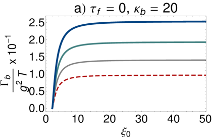
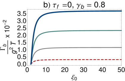
Figure 5: (color online). The $\xi_{0}$ dependence of $\frac{\Gamma_{b}}{g^{2}T}$ for $\tau_{f}=0$ and (a) $\kappa_{b}=20$ as well as $\gamma_{b}=0.5,0.6,0.7,0.8$ (from below to above) and (b) $\gamma_{b}=0.8$ as well as $\kappa_{b}=1,2,3,4$ (from below to above). As it turns out, $\frac{\Gamma_{b}}{g^{2}T}$ remains constant for $\xi_{0}\gtrsim 10$. For fixed values of $\xi_{0}$ and $\kappa_{b}$ ($\gamma_{b}$), $\frac{\Gamma_{b}}{g^{2}T}$ increases with increasing $\gamma_{b}$ ($\kappa_{b}$) [see panel a (b)].

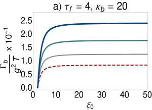
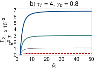
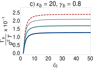
Figure 6: (color online). The $\xi_{0}$ dependence of $\frac{\Gamma_{b}}{g^{2}T}$ for $\tau_{f}=4$ and (a) $\kappa_{b}=20$ as well as $\gamma_{b}=0.5,0.6,0.7,0.8$ (from below to above), and (b) $\gamma_{b}=0.8$ as well as $\kappa_{b}=1,2,3,4$ (from below to above). As it turns out, $\frac{\Gamma_{b}}{g^{2}T}$ remains constant for $\xi_{0}\gtrsim 10$. For a fixed value of $\xi_{0}$, $\frac{\Gamma_{b}}{g^{2}T}$ increases with increasing $\gamma_{b}$ for all values of $\kappa_{b}$ (panel a) and with increasing $\kappa_{b}$ for all values of $\gamma_{b}$ (panel b). (c) The $\xi_{0}$ dependence of $\frac{\Gamma_{b}}{g^{2}T}$ for fixed $\kappa_{b}=20,\gamma_{b}=0.8$ and $\tau_{f}=4,6,8,10$ (from above to below). As in the previous cases, $\frac{\Gamma_{b}}{g^{2}T}$ remains constant for $\xi_{0}\gtrsim 10$ for all values of $\kappa_{b},\gamma_{b}$ and $\tau_{f}$. For a fixed value of $\kappa_{b},\gamma_{b}$ and $\xi_{0}$, $\frac{\Gamma_{b}}{g^{2}T}$ decreases with increasing $\tau_{f}$.

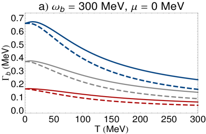
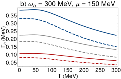
Figure 7: (color online). The $T$ dependence of $\Gamma_{b}$ for $\omega_{b}=300$ MeV and (a) $\mu=0$ MeV as well as (b) $\mu=150$ MeV. The red, gray and blue lines correspond to $m_{b}^{0}=100,150,200$ MeV and $m_{f}^{0}=5$ MeV, respectively. The dashed lines include only the constant mass contributions of bosons, $m_{b}^{0}=100,150,200$ MeV, and fermions $m_{f}^{0}=5$ MeV. The solid lines include, in addition to the constant mass contributions, the thermal corrections of the boson and fermion masses as functions of $T$ and $\mu$ [see (V) to (V)]. Here, the Yukawa coupling $g=0.5$ is used.

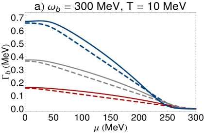
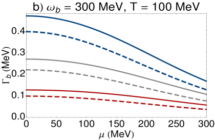
Figure 8: (color online). The $\mu$ dependence of $\Gamma_{b}$ for $\omega_{b}=300$ MeV and (a) $T=10$ MeV as well as (b) $T=100$ MeV. The red, gray and blue lines correspond to $m_{b}^{0}=100,150,200$ MeV and $m_{f}^{0}=5$ MeV, respectively. The dashed lines include only the constant mass contributions of bosons, $m_{b}^{0}=100,150,200$ MeV, and fermions, $m_{f}^{0}=5$ MeV. The solid lines include, in addition to the constant mass contributions, the thermal corrections of the boson and fermion masses as functions of $T$ and $\mu$ [see (V) to (V)]. Here, the Yukawa coupling $g=0.5$ is used.

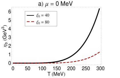
Figure 9: (color online). (a) The $T$ dependence of $\eta_{b}$ is plotted for $\mu=0$ and $T$ independent $\xi_{0}=40,80$ arising from $m_{b}^{0}=200,400$ MeV and $m_{f}^{0}=5$ MeV. (b) The $T$ dependence of $\eta_{b}$, including the $T$ dependent thermal corrections to bosonic and fermionic masses, is plotted for $m_{b}^{0}=200,400$ MeV and $m_{f}^{0}=5$ MeV. Here, $\xi_{0}^{T}$ denotes the ratio $m_{b}^{0}/m_{f}^{0}$ in $\xi(T,\mu)$ from (V.2) and (V).

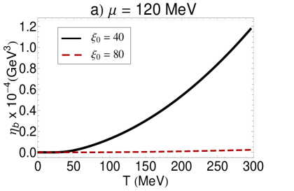
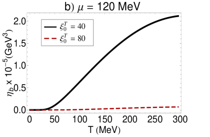
Figure 10: (color online). (a) The $T$ dependence of $\eta_{b}$ is plotted for $\mu=120$ MeV and $(T,\mu)$ independent $\xi_{0}=40,80$ arising from $m_{b}^{0}=200,400$ MeV and $m_{f}^{0}=5$ MeV. (b) The $T$ dependence of $\eta_{b}$, including the $T$ and $\mu$ dependent thermal corrections to bosonic and fermionic masses, is plotted for $m_{b}^{0}=200,400$ MeV and $m_{f}^{0}=5$ MeV, leading to $\xi_{0}^{T}=40,80$.

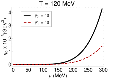
Figure 11: (color online). The $\mu$ dependence of $\eta_{b}$ is plotted for $T=120$ MeV and $\xi_{0}=\xi_{0}^{T}=40$.

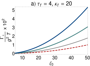
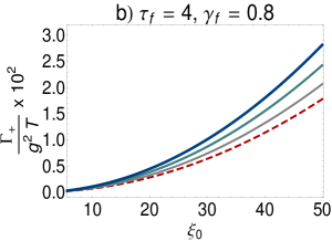
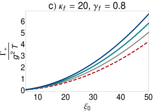
Figure 12: (color online). The $\xi_{0}$ dependence of $\frac{\Gamma_{+}}{g^{2}T}$ for $\tau_{f}=4$ and (a) $\kappa_{f}=20$ as well as $\gamma_{f}=0.5,0.6,0.7,0.8$ (from below to above), and (b) $\gamma_{f}=0.8$ as well as $\kappa_{f}=2,4,6,8$ (from below to above).(c) The $\xi_{0}$ dependence of $\frac{\Gamma_{+}}{g^{2}T}$ for $\kappa_{f}=20,\gamma_{f}=0.8$ and $\tau_{f}=0,3,6,9$ (from below to above). As it turns out, for a fixed $\xi_{0}$, $\frac{\Gamma_{+}}{g^{2}T}$ increases whenever one of the parameters $\gamma_{f},\kappa_{f}$ or $\tau_{f}$ increases and the other two parameters are held fixed. It can be shown that the same is also true for $\frac{\Gamma_{-}}{g^{2}T}$.

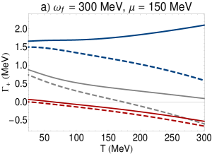
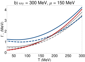
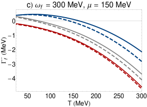
Figure 13: (color online). The $T$ dependence of (a) $\Gamma_{+}$ (b) $\Gamma_{-}$ and (c) $\Gamma_{f}^{-}=\Gamma_{+}-\Gamma_{-}$ is plotted for constant $\omega_{f}=300$ MeV and $\mu=150$ MeV. The red, gray and blue solid and dashed lines correspond to $m_{b}^{0}=300,450,600$ MeV and $m_{f}^{0}=5$ MeV. Whereas the dashed lines correspond to $\Gamma_{\pm}$ and $\Gamma_{f}^{-}$ as functions of $(T,\mu)$ independent $\xi_{0}=60,90,120$, the solid lines correspond to the same quantities including the thermal corrections to bosonic and fermionic masses with $\xi_{0}^{T}=60,90,120$. It turns out that the absolute value of the difference between $\Gamma_{+}$ and $\Gamma_{-}$, i.e. $|\Gamma_{f}^{-}|$, increases with increasing $T$, and decreases with increasing $\xi_{0}$ and $\xi_{0}^{T}$. Moreover, for small $\xi_{0}$ or $\xi_{0}^{T}$ and fixed $(T,\mu)$, $\Gamma_{-}$ is always larger than $\Gamma_{+}$.

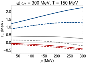
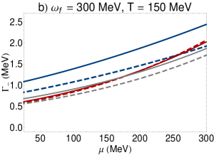
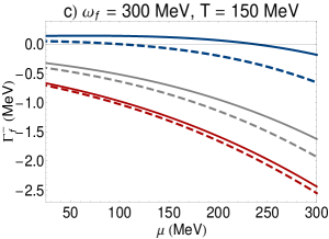
Figure 14: (color online). The $\mu$ dependence of (a) $\Gamma_{+}$ (b) $\Gamma_{-}$ and (c) $\Gamma_{f}^{-}=\Gamma_{+}-\Gamma_{-}$ is plotted for constant $\omega_{f}=300$ MeV and $T=150$ MeV. The red, gray and blue solid and dashed lines correspond to $m_{b}^{0}=300,450,600$ MeV and $m_{f}^{0}=5$ MeV. Whereas the dashed lines correspond to $\Gamma_{\pm}$ and $\Gamma_{f}^{-}$ as functions of $(T,\mu)$ independent $\xi_{0}=60,90,120$, the solid lines correspond to the same quantities including the thermal corrections to bosonic and fermionic masses with $\xi_{0}^{T}=60,90,120$. Similar to their $T$ dependence, demonstrated in Fig. 13, it turns out that $|\Gamma_{f}^{-}|$ increases with increasing $\mu$, and decreases with increasing $\xi_{0}$ as well as $\xi_{0}^{T}$. Moreover, for small $\xi_{0}$ or $\xi_{0}^{T}$ and fixed $(T,\mu)$, $\Gamma_{-}$ is always larger than $\Gamma_{+}$.

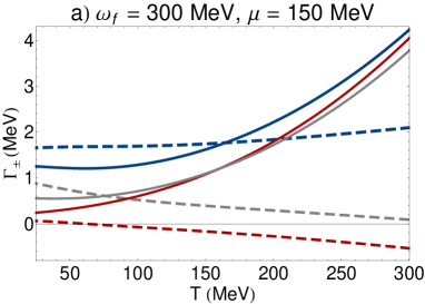
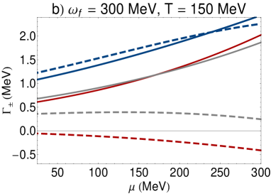
Figure 15: (color online). (a) The $T$ dependence of $\Gamma_{\pm}$ for $\omega_{f}=300$ MeV and $\mu=150$ MeV, including the thermal corrections to bosonic and fermionic masses. (b) The $\mu$ dependence of $\Gamma_{\pm}$ for $\omega_{f}$ MeV and $T=150$ MeV, including the thermal corrections to bosonic and fermionic masses. The dashed (solid) lines correspond to $\Gamma_{+}$ ($\Gamma_{-}$). The red, gray and blue dashed and solid lines correspond to $\xi_{0}^{T}=60,90$ and $\xi_{0}^{T}=120$, respectively.

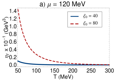
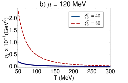
Figure 16: (color online). The $T$ dependence of $\eta_{f}$ is plotted for $\mu=120$ MeV and $T$ independent $\xi_{0}=40,80$ arising from $m_{b}^{0}=200,400$ MeV and $m_{f}^{0}=5$ MeV. (b) The $T$ dependence of $\eta_{f}$, including the $T$ and $\mu$ dependent thermal corrections to bosonic and fermionic masses, is plotted for $m_{b}^{0}=200,400$ MeV and $m_{f}^{0}=5$ MeV, leading to $\xi_{0}^{T}=40,80$.

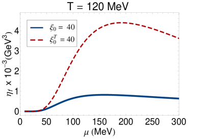
Figure 17: (color online). The $\mu$ dependence of $\eta_{f}$ is plotted for $T=120$ MeV and $\xi_{0}=\xi_{0}^{T}=40$.

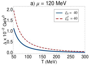
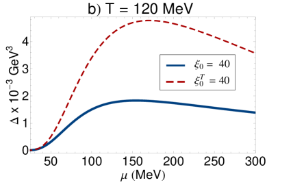
Figure 18: (color online). (a) The $T$ dependence of $\Delta$, defined in (V.4), is plotted for $\mu=120$ MeV and $\xi_{0}=\xi_{0}^{T}=40$. (b) The $\mu$ dependence of $\Delta$ is plotted for $T=120$ MeV and $\xi_{0}=\xi_{0}^{T}=40$. As it turns out, $\Delta$ decreases (increases) with increasing $T$ ($\mu$) and constant mass ratio $\xi_{0}$ as well as $\xi_{0}^{T}$.

Let us first consider (IV.18) and (C.16), where the bosonic spectral width $\Gamma_{b}$ is presented as a function of dimensionless parameters, $\gamma_{b}=\frac{m_{b}}{\omega_{b}},\kappa_{b}=\omega_{b}/T$ with $\omega_{b}^{2}=\mathbf{p}^{2}+m_{b}^{2}$ and $\xi=\frac{m_{b}}{m_{f}}$ as well as $\tau_{f}=\mu/T$ for $\mu=0$ (IV.18) and $\mu\neq 0$ (C.16). We consider first the constant mass approach, and replace all $m_{b}$ and $m_{f}$ with $m_{b}^{0}$ and $m_{f}^{0}$, respectively. We then focus on the $\xi_{0}$ dependence of $\Gamma_{b}$ for fixed $\kappa_{b},\gamma_{b}$ and $\tau_{f}$. In Fig. 5(a), the $\xi_{0}$ dependence of dimensionless quantity $\frac{\Gamma_{b}}{g^{2}T}$ is plotted for $\tau_{f}=0$ and $\kappa_{b}=20$ as well as $\gamma_{b}=0.5,0.6,0.7,0.8$ [from below (red dashed line) to above (blue solid line)]. In Fig. 5(b), the $\xi_{0}$ dependence of $\frac{\Gamma_{b}}{g^{2}T}$ is plotted for $\tau_{f}=0$ and $\gamma_{b}=0.8$ as well as $\kappa_{b}=1,2,3,4$ [from below (red dashed line) to above (blue solid line)]. We observe that $\frac{\Gamma_{b}}{g^{2}T}$ remains constant for $\xi_{0}\gtrsim 10$ in both cases. Moreover, for fixed values of $\xi_{0}$ and $\kappa_{b}$ ($\gamma_{b}$), the ratio $\frac{\Gamma_{b}}{g^{2}T}$ increases with increasing $\gamma_{b}$ ($\kappa_{b}$) [see panels (a) and (b) of Fig. 5].

In Fig. 6(a), the $\xi_{0}$ dependence of $\frac{\Gamma_{b}}{g^{2}T}$ is plotted for $\tau_{f}=4$ and $\kappa_{b}=20$ as well as $\gamma_{b}=0.5,0.6,0.7,0.8$ [from below to above]. In Fig. 6(b), the same dimensionless quantity is plotted for $\tau_{f}=4$ and $\gamma_{b}=0.8$ as well as $\kappa_{b}=1,2,3,4$ [from below to above]. Similar to the case of $\tau_{f}=0$, $\frac{\Gamma_{b}}{g^{2}T}$ remains constant for $\xi_{0}\gtrsim 10$, and increases with increasing $\gamma_{b}(\kappa_{b})$ for fixed values of $\xi_{0}$ and $\kappa_{b}$ ($\gamma_{b}$). In Fig. 6(c), the $\xi_{0}$ dependence of $\frac{\Gamma_{b}}{g^{2}T}$ is plotted for fixed $\kappa_{b}=20$ and $\gamma_{b}=0.8$ as well as $\tau_{f}=4,6,8,10$ [from above (red dashed line) to below (blue solid line)]. In contrast to the previous cases, $\frac{\Gamma_{b}}{g^{2}T}$ decreases with increasing $\tau_{f}$ and fixed $\kappa_{b},\gamma_{b}$ and $\xi_{0}$. These results indicate that $\Gamma_{b}$ decreases with increasing $T$ and/or $\mu$. This conclusion is compatible with the observed result demonstrated in Figs. 7 and 8, where the $T$ and $\mu$ dependence of $\Gamma_{b}$ is studied for various fixed parameters.

In Fig. 7, the $T$ dependence of $\Gamma_{b}$ is plotted for $\omega_{b}=300$ MeV, $m_{f}^{0}=5$ MeV and $\mu=0$ MeV [Fig. 7(a)] as well as $\mu=150$ MeV [Fig. 7(b)]. The Yukawa coupling is chosen to be $g=0.5$. Similarly, in Fig. 8, the $\mu$ dependence of $\Gamma_{b}$ is plotted for $\omega_{b}=300,m_{f}^{0}=5$ MeV and $T=10$ MeV [Fig. 8(a)] as well as $T=100$ MeV [Fig. 8(b)]. The red, gray and blue lines in Figs. 7 and 8 correspond to $m_{b}^{0}=100,150$ and $200$ MeV, respectively. The dashed lines include the contributions of constant masses $m_{b}^{0}$ and $m_{f}^{0}$ for bosons and fermions, respectively, and the solid lines include the contributions of thermal corrections of fermion and boson masses, $m_{b}(T,\mu)$ and $m_{f}(T,\mu)$ from (V). As it turns out, $\Gamma_{b}$ decreases with increasing $T$ and $\mu$. Having in mind that $\Gamma_{b}^{-1}$ is essentially proportional to the mean free path of the bosons, $\lambda_{b}$, lang2012 , the fact that $\Gamma_{b}$ decreases with increasing $T$ and $\mu$ means that $\lambda_{b}$ increases with increasing $T$ and $\mu$. However, for constant $T$ and $\mu$, heavier bosons seems to have smaller $\lambda_{b}$, as expected. Although, according to Figs. 7 and 8, adding $T$ and $\mu$ dependent (thermal) masses of bosons and fermions to the bare masses $m_{b}^{0}$ and $m_{f}^{0}$ shifts $\Gamma_{b}$ to larger values, but the qualitative interpretation concerning $\lambda_{b}$ remains unchanged. According to (III.1), indicating that $\eta_{b}\sim\Gamma_{b}^{-1}$, the thermal behavior of $\lambda_{b}$ is expected to be reflected in thermal behavior of $\eta_{b}$, as it will be shown below.

V.1.2 Bosonic part of the shear viscosity

The bosonic part of the shear viscosity is presented in (III.1), with $\Gamma_{b}$ given in (IV.18) for $\mu=0$ and (C.16) for $\mu\neq 0$. To determine $\eta_{b}$, we neglect the contribution of $\mathfrak{Re}[\Sigma_{R}^{b}(p)]$ in $E_{b}$ from (III.19) and set $E_{b}\sim\omega_{b}$. In Fig. 9, the $T$ dependence of $\eta_{b}$ is plotted for $\mu=0$. The black solid and red dashed lines in Fig. 9(a) correspond to constant ratio $\xi_{0}=40$ MeV and $\xi_{0}=80$ MeV. The latter arise from $m_{b}^{0}=200,400$ MeV and $m_{f}^{0}=5$ MeV, respectively. In Fig. 9(b), the $T$ dependence of $\eta_{b}$ is plotted for $\mu=0$. But, in this case, in contrast to the plot in Fig. 9(a), $\eta_{b}$ includes thermal masses $m_{b}(T,\mu)$ and $m_{f}(T,\mu)$ from (V) with $m_{b}^{0}=200,400$ MeV and $m_{f}^{0}=5$ MeV. In Fig. 9(b), $\xi_{0}^{T}$ denotes the ratio $m_{b}^{0}/m_{f}^{0}$ in $\xi(T,\mu)$ from (V.2). In Figs. 10(a) and (b), the same quantities are plotted for $\mu=120$ MeV. Comparing the plots of $\eta_{b}$ for different constant masses in Figs. 9(a) and 10(a), it turns out that $\eta_{b}$ decreases with increasing $\xi_{0}$. The same is also true for $\xi(T,\mu)$ [see Figs. 9(b) and 10(b)]. These results are compatible with our findings in Figs. 7(a) and 7(b), since for constant $T$ and $\mu$, $\eta_{b}$ is approximately proportional to $\Gamma_{b}^{-1}$ [see (III.1)]. Moreover, as expected from Fig. 7, $\eta_{b}$ increases with increasing $T$. Comparing the results for constant and $(T,\mu)$ dependent masses in Figs. 9 and 10, it turns out that, as expected from Fig. 7, adding the thermal corrections to the constant bosonic and fermionic masses decreases the value of $\eta_{b}$. Moreover, for both constant and $T$ or/and $\mu$ dependent masses, the difference between $\eta_{b}$ for different $\xi_{0}$ as well as $\xi_{0}^{T}$ increases with increasing $T$. However, since the scales in the plots of Fig. 9 and Fig. 10 are different, the difference between $\eta_{b}$ for $\xi_{0}$ and $\xi_{0}^{T}$ seems to be negligible for the case $\mu\neq 0$ comparing to the case $\mu=0$. When we compare the plots of Fig. 9 with the plots of Fig. 10, it seems that $\eta_{b}$ decreases with increasing $\mu$. This conclusion contradicts the result from Figs. 7 and 8, together with the fact that $\eta_{b}\sim\Gamma_{b}^{-1}$ from (III.1). This apparent contradiction may lie on the fact that for $\mu\neq 0$, the $p$-integration in (III.1) is taken in the interval $p\in[0,(\mu^{2}-m_{f}^{0~{}2})^{1/2}]$ for constant fermionic mass $m_{f}^{0}$, and $p\in[0,[\mu^{2}-m_{f}^{2}(T,\mu)]^{1/2}]$, with $(T,\mu)$ dependent fermionic mass $m_{f}(T,\mu)$ from (V). Hence, the $\mu$ dependence of $\Gamma_{b}$ is not the only source for the $\mu$ dependence of $\eta_{b}$. In Fig. 11, the $\mu$ dependence of $\eta_{b}$ is demonstrated for constant $T=120$ MeV and $\xi_{0}=40$ as well as $(T,\mu)$ dependent $\xi(T,\mu)$ with $\xi_{0}^{T}=40$. As expected from Figs. 7 and 8, $\eta_{b}$ increases with increasing $\mu$. Recently, in sarkar2013 , the shear viscosity of a hot pion gas, $\eta_{\pi}$, is determined by solving the relativistic transport equation in Chapman-Enskog and relaxation time approximations. It is shown that for zero pion chemical potential, $\eta_{\pi}$ increases with $T$. Although the setup discussed in sarkar2013 is slightly different from ours – the self-interaction of pseudoscalar pions is described by the Lagrangian density of chiral perturbation theory – our results for zero $\mu$ and finite $T$ coincide with the results presented in sarkar2013 . The fact that, according to our results from Figs. 9-11, $\eta_{b}$ increases also with $T$ or $\mu$, shows that $T$ and $\mu$ have the same effect on the bosons propagating in a dissipative hot and dense medium. As we have argued in the previous section, the mean free path of bosons, $\lambda_{b}$ increases with increasing $T$ and/or $\mu$. The results of the present section shows that the thermal properties of $\lambda_{b}$ is directly reflected in the thermal properties of $\eta_{b}$. Moreover, as it turns out heavier bosons have smaller $\eta_{b}$ and $\lambda_{b}$, as expected.

V.2 Fermionic contributions

V.2.1 Fermionic spectral width

In this section, we will focus on the $T$ and $\mu$ dependence of the fermionic spectral widths $\Gamma_{\pm}$, with the emphasis on the difference between them. As aforementioned, in the chiral limit $m_{f}\to 0$ and at finite $(T,\mu)$, $\Gamma_{+}$ and $\Gamma_{-}$ correspond to the normal and collective excitations of fermions, respectively. The latter is referred to either as a hole or as a plasmino. Moreover, in the chiral limit, $\Gamma_{+}$ ($\Gamma_{-}$) corresponds to excitations with the same (opposite) chirality and helicity. The difference between $\Gamma_{+}$ and $\Gamma_{-}$ is often neglected in the literature jeon2007 . We, however, highlight this difference and study its impact on the fermionic shear viscosity in different regimes of temperature and chemical potential.

In (IV.2) and (C.2), $\Gamma_{+}$ is presented for vanishing and non-vanishing $\mu$ in terms of dimensionless parameters $\gamma_{f}=\frac{m_{f}}{\omega_{f}},\kappa_{f}=\omega_{f}/T$ with $\omega_{f}^{2}=\mathbf{p}^{2}+m_{f}^{2}$ and $\xi=\frac{m_{b}}{m_{f}}$ as well as $\tau_{f}=\mu/T$. Similarly, $\Gamma_{f}^{-}(\gamma_{f},\kappa_{f},\tau_{f};\xi)$ for $\mu=0$ and $\mu\neq 0$ are presented in (B) and (C.2), respectively. Using $\Gamma_{-}=\Gamma_{+}-\Gamma_{f}^{-}$, $\Gamma_{-}$ can be determined from the difference between $\Gamma_{+}$ and $\Gamma_{f}^{-}$. Similar to the bosonic case, let us replace $m_{b}$ and $m_{f}$ with $(T,\mu)$ independent $m_{b}^{0}$ and $m_{f}^{0}$, respectively, and focus first on the $\xi_{0}=m_{b}^{0}/m_{f}^{0}$ dependence of the dimensionless quantity $\frac{\Gamma_{+}}{g^{2}T}$ as a function of dimensionless parameters $\gamma_{f},\kappa_{f}$ and $\tau_{f}$.

In Fig. 12(a), the $\xi_{0}$ dependence of $\frac{\Gamma_{+}}{g^{2}T}$ is plotted for fixed $\tau_{f}=4$ and $\kappa_{f}=20$ as well as $\gamma_{f}=0.5,0.6,0.7,0.8$ [from below (red dashed line) to above (blue solid line)]. Similarly, in Fig. 12(b), the $\xi_{0}$ dependence of $\frac{\Gamma_{+}}{g^{2}T}$ is plotted for $\tau_{f}=4$ and $\gamma_{f}=0.8$ as well as $\kappa_{f}=2,4,6.8$ [from below (red dashed line) to above (blue solid line)]. Finally, in Fig. 12(c), the $\xi_{0}$ dependence of $\frac{\Gamma_{+}}{g^{2}T}$ is plotted for fixed $\kappa_{f}=20$ and $\gamma_{f}=0.8$ as well as $\tau_{f}=0,3,6,9$ [from below (red dashed line) to above (blue solid line)]. In contrast to the bosonic case, for a fixed $\xi_{0}$, $\frac{\Gamma_{+}}{g^{2}T}$ increases whenever one of the parameters $\gamma_{f},\kappa_{f}$ or $\tau_{f}$ increases and the other two parameters are held fixed. Neglecting the tiny difference between $\frac{\Gamma_{+}}{g^{2}T}$ and $\frac{\Gamma_{-}}{g^{2}T}$, the same can easily be shown to be true for $\frac{\Gamma_{-}}{g^{2}T}$. Let us notice at this stage, that to derive the final results for $\Gamma_{\pm}$ for $\mu=0$ and $\mu\neq 0$, the condition $m_{b}^{0}\geq 2m_{f}^{0}$ was necessary. It is easy to show that $\Gamma_{\pm}$ diverges once $m_{b}^{0}=m_{f}^{0}=0$. This is also indicated in plasmino-yukawa-2 , where it is noted that nonzero boson and fermion mass difference, $\delta m^{2}=m_{b}^{2}-m_{f}^{2}$, ensures the smoothness of the fermion self-energy, and consequently $\Gamma_{\pm}$, in the far infrared (IR) limit.

Although the $\xi_{0}$ dependence of $\frac{\Gamma_{+}}{g^{2}T}$ and $\frac{\Gamma_{-}}{g^{2}T}$ as functions of dimensionless parameters $\gamma_{f},\kappa_{f}$ and $\tau_{f}$ are practically identical, the $T$ ($\mu$) dependence of $\Gamma_{+}$ and $\Gamma_{-}$ turns out to be different for fixed value of $\mu$ ($T$) and $\xi_{0}$. In Figs. 13 and 14, the $T$ and $\mu$ dependence of $\Gamma_{+}$ (panel a), $\Gamma_{-}$ (panel b) as well as $\Gamma_{f}^{-}$ (panel c) are plotted for $\omega_{f}=300$ MeV and $\mu=150$ MeV (Fig. 13), as well as for $\omega_{f}=300$ MeV and $T=150$ MeV (Fig. 14). The red, gray and blue solid and dashed lines correspond to $m_{b}^{0}=300,450,600$ MeV and $m_{f}^{0}=5$ MeV. The dashed lines correspond to $\Gamma_{\pm}$ and $\Gamma_{f}^{-}$ as functions of $(T,\mu)$ independent $\xi_{0}=60,90,120$, and the solid lines correspond to the same quantities, including the thermal masses of bosons and fermions, with $\xi_{0}^{T}=m_{b}^{0}/m_{f}^{0}=60,90,120$. According to the results in Figs. 13 and 14, it turns out that the absolute value of the difference between $\Gamma_{+}$ and $\Gamma_{-}$, $|\Gamma_{f}^{-}|$, increases with increasing $T$ and constant $\mu$ (Fig. 13), as well as with increasing $\mu$ and constant $T$ (Fig. 14). It decreases with increasing $\xi_{0}$ and $\xi_{0}^{T}$. Moreover, for small value of $\xi_{0}$ or $\xi_{0}^{T}$ and fixed $(T,\mu)$, $\Gamma_{-}$ is always larger than $\Gamma_{+}$.

To compare $\Gamma_{+}$ and $\Gamma_{-}$ more directly, their $T$ and $\mu$ dependence are plotted in Fig. 15 for constant $\omega_{f}=300$ MeV and $\mu=150$ MeV (panel a) and $T=150$ MeV. Here, $\Gamma_{\pm}$ include only thermal bosonic and fermionic masses. The dashed (solid) lines correspond to $\Gamma_{+}$ ($\Gamma_{-}$). The red, gray and blue dashed and solid correspond to $\xi_{0}^{T}=60,90,120$, respectively. As it turns out, whereas for smaller $\xi_{0}^{T}=m_{b}^{0}/m_{f}^{0}$, $\Gamma_{+}$, the spectral width of normal fermion excitations, decreases with $T$ or $\mu$, for larger $\xi_{0}^{T}$, it increases with increasing $T$ or $\mu$. In contrast, $\Gamma_{-}$, the spectral width of the plasmino excitations, increases with $T$ or $\mu$, independent of $\xi_{0}^{T}$. Assuming, in analogy to the bosonic case, that the spectral widths $\Gamma_{+}$ and $\Gamma_{-}$ are inversely proportional to the mean free paths of the normal and plasmino excitations of the fermions, $\lambda_{+}$ and $\lambda_{-}$, the above results suggest that at higher temperature or chemical potential, plasminos have smaller $\lambda_{-}$, while for normal fermions, the thermal behavior of $\lambda_{+}$ depends strongly on the relation between the masses of the fermions and bosons included in our Yukawa-Fermi gas. Heavier (normal) fermions have smaller $\lambda_{+}$, as expected. Let us eventually mention that, according to the plots in Figs. 13 and 14, $|\Gamma_{f}^{-}|=|\Gamma_{+}-\Gamma_{-}|$ increases with increasing $T$ ($\mu$) and fixed $\mu$ ($T$), as suggested from the fact that holes (plasminos) are more significant at higher temperature weldon1989 . In what follows, we will study the impact of this difference on the fermionic part of the shear viscosity.

V.2.2 Fermionic part of the shear viscosity

In Sec. III.2, the fermionic part of the shear viscosity, $\eta_{f}$, is computed in terms of $\Gamma_{+}$ and $\Gamma_{-}$ for vanishing chemical potential [see (III.2)]. In App. C, we presented $\eta_{f}$ for non-vanishing chemical potential [see (C.1)]. Neglecting the contribution of $\mathfrak{Re}[\Sigma_{R}^{f}]$ in $E_{\pm}$ from (III.2) and in ${\cal{E}}_{\pm}$ from (C.1), and replacing $E_{\pm}$ and ${\cal{E}}_{\pm}$, appearing in (III.2) and (C.1), with $\omega_{f}$ and $\omega_{\pm}=\omega_{f}\pm\mu$, respectively, we have plotted the $T$ dependence of $\eta_{f}$ for fixed $\mu=120$ MeV and $\xi_{0}=40,80$ in Fig. 16(a) and for $\mu=120$ MeV and $\xi_{0}^{T}=40,80$ in Fig. 16(b). In contrast to the $T$ dependence of $\eta_{b}$ from Fig. 10, we observe that $\eta_{f}$ decreases with increasing $T$, $\eta_{f}$ is in general larger than $\eta_{b}$, and at a fixed temperature and for a fixed chemical potential, $\eta_{f}$ increases with increasing $\xi_{0}$ [Fig. 16(a)] as well as $\xi_{0}^{T}$ [Fig. 16(b)]. The fact that for a fixed $T$ and $\mu$, $\eta_{f}$ decreases with increasing $\xi_{0}$ is compatible with the results arising from Fig. 12, where it is shown that $\Gamma_{\pm}$ increases with increasing $\xi_{0}$, and confirms the fact that for small values of $\xi_{0}$ (or $\xi_{0}^{T}$), $\eta_{f}\sim\Gamma_{\pm}^{-1}$. But, in general, it seems that the thermal property of $\eta_{f}$ is dominated by the thermal behavior of $\Gamma_{-}$. The fact that $\eta_{f}$ is inversely proportional to the fermionic spectral width coincides with the results presented in plasmino-NJL , and indicates that $\eta_{f}$ increases with increasing the mean free path.

In Fig. 17, the $\mu$ dependence of $\eta_{f}$ is plotted for $T=120$ MeV and $\xi_{0}=40$ (blue solid line) and $\xi_{0}^{T}=40$ (red dashed line). In contrast to the $\mu$ dependence of $\eta_{b}$ from Fig. 11, $\eta_{f}$ decreases with increasing $\mu$ at a fixed temperature. Moreover, at a fixed $T$ and $\mu$, $\eta_{f}$ decreases when the thermal corrections to the bosonic and fermionic masses are taken into account. This is again in contrast with the observed results for $\eta_{b}$ in Fig. 11.

As we have shown in Figs. 13, 14 and 15, $\Gamma_{+}$ and $\Gamma_{-}$ have different thermal properties. To study how this difference can affect $\eta_{f}$, we define a quantity $\Delta$, as the difference between $\eta_{f}$ as a functional of $\Gamma_{+}=\Gamma_{-}$, and $\eta_{f}$ as a functional of $\Gamma_{+}\neq\Gamma_{-}$,

$$\Delta=\eta_{f}[\Gamma_{+}=\Gamma_{-}]-\eta_{f}[\Gamma_{+}\neq\Gamma_{-}].$$ (V.4)

Let us remind, that in the literature the difference between $\Gamma_{+}$ and $\Gamma_{-}$ is often neglected, and in so far, $\Delta\simeq 0$ is assumed. In Figs. 18(a) and (b), the $T$ and $\mu$ dependence of $\Delta$ is plotted for constant $\mu=120$ MeV (panel a) and $T=120$ MeV (panel b), and for $\xi_{0}=40$ (blue solid lines) and $\xi_{0}^{T}=40$ (red dashed lines). It turns out that in the whole range of $T$ and $\mu$, $\Delta$ is positive. This means that the value of $\eta_{f}$ increases, when the difference between $\Gamma_{+}$ and $\Gamma_{-}$ is neglected. Moreover, for fixed $\mu$ (T) and constant $\xi_{0}$ or $\xi_{0}^{T}$, $\Delta$ decreases (increases) with $T$ ($\mu$). In other word, as it is shwon in Fig. 18(a), whereas at lower temperature and for an intermediate value of $\mu$, the difference between $\eta_{f}[\Gamma_{+}=\Gamma_{-}]$ and $\eta_{f}[\Gamma_{+}\neq\Gamma_{-}]$ is relatively large, and becomes larger by including the thermal corrections to the bosonic and fermionic masses, it can be neglected at higher temperature. In contrast, the difference between $\eta_{f}[\Gamma_{+}=\Gamma_{-}]$ and $\eta_{f}[\Gamma_{+}\neq\Gamma_{-}]$ is negligible at fixed temperature and for small value of chemical potential. It increases with increasing $\mu$ and is enhanced by adding the thermal corrections to the bosonic and fermionic masses.

VI Summary and outlook

The shear viscosity $\eta$ is a transport coefficient, that characterizes the diffusion of momentum transverse to the direction of propagation. It plays an important rôle in the physics of QGP. In the past few years, there have been several attempts to explore its thermal properties, in particular in the vicinity of QCD chiral transition point. The aim is to determine the position of the transition temperature of QCD, using the thermal properties of $\eta$, in addition to and independently of the equation of state kapusta2008 . In this paper, we studied the thermal properties of the shear viscosity of an interacting boson-fermion system with Yukawa coupling. We followed the method presented in lang2012 to derive the bosonic part of the shear viscosity of this theory in terms of the bosonic spectral width, $\Gamma_{b}$. The latter is then determined in a one-loop perturbative expansion in the orders of the Yukawa coupling. Using $\eta_{b}[\Gamma_{b}]$, it was then possible to study the thermal properties of $\eta_{b}$, in addition to its dependence to the masses of bosons and fermions.

We took the method used in lang2012 , as our guideline, and determined the fermionic part of the shear viscosity of the Yukawa theory in terms of the fermionic widths $\Gamma_{+}$ and $\Gamma_{-}$. The expression $\eta_{f}[\Gamma_{\pm}]$ from (III.2) and (C.1) for vanishing and non-vanishing chemical potential, build the central analytical results of the present paper. Here, $\Gamma_{+}$ and $\Gamma_{-}$ are the spectral widths, corresponding to the normal and collective (plasmino) excitations of fermions. They are studied very intensively in the literature and lead e.g. to structures in the low mass dilepton production rate, which might provide a unique signature for the QGP formation at relativistic heavy ion collisions plasmino-app . However, to the best of our knowledge, the difference between their spectral widths is often neglected (see e.g. in nardi2009 ; kiessig2010 ; plasmino-yukawa-1 ), and, as in jeon2007 ; lang2013 , the fermionic spectral density function, $\rho_{f}$, is given in terms of one and the same fermionic spectral width. We, however, used the structure of $\rho_{f}$ presented in plasmino-NJL , including both $\Gamma_{+}$ and $\Gamma_{-}$, and following the method presented in lang2012 , determined $\eta_{f}[\Gamma_{\pm}]$ in an appropriate Laurent expansion. Moreover, we completed the results presented in plasmino-NJL , and evaluated first $\Gamma_{\pm}$ in one-loop perturbative expansion in the orders of the Yukawa coupling, and studied their thermal properties. Plugging then $\Gamma_{\pm}$ in the proposed relation for the fermionic shear viscosity, $\eta_{f}[\Gamma_{\pm}]$ from (III.2) and (C.1), we determined the thermal properties of $\eta_{f}$, and studied its mass dependence. Apart from various results on the thermal properties of $\Gamma_{b},\Gamma_{\pm}$ as well as $\eta_{b}$ and $\eta_{f}$, discussed in the previous section, we showed that, depending on temperature and/or chemical potential, $\eta_{f}[\Gamma_{+}\neq\Gamma_{-}]$ is smaller than $\eta_{f}[\Gamma_{+}=\Gamma_{-}]$.

It shall be noted that our one-loop computation, including bare fermion and boson masses, is incomplete and can be improved, for instance, by considering the full HTL correction to the fermion propagator. The latter plays a crucial rôle in determining $\Gamma_{b}$ and $\Gamma_{\pm}$, and consequently $\eta_{b}$ and $\eta_{f}$. This drawback is partly compensated in the present paper by adding thermal corrections to the bosonic and fermionic masses. This ad-hoc treatment of thermal masses seems to be natural, since, as it is also discussed in kiessig2009 ; kiessig2010 , it equals the HTL treatment with an approximate fermion propagator. Moreover, since it is known that the HTL/HDL treatment are only valid for soft momenta $p\lesssim gT,g\mu$, even the HTL treatment can be improved by studying the ultra-soft fermionic excitations, with $p\lesssim g^{2}T,g^{2}\mu$. They are recently discussed in plasmino-yukawa-2 ; balizot2014 , in the framework of the Yukawa theory. An important question related to the perturbative treatment of transport coefficients, in general, and shear viscosity, in particular, is the appearance of the so called pinch singularities, that would break the perturbation theory based on loop expansion. A useful description of these singularities is presented in hidaka2010 : In the quasiparticle approximation, where the propagators are given by the energy and spectral widths of the quasiparticles, the pinch singularity is essentially related to the IR behavior of the product of retarded and advanced propagators, that appears in the perturbative loop calculations. Once the spectral width is zero, the above mentioned product becomes IR divergent. The consequence is that higher loop diagrams, if they are sufficiently IR sensitive, become as important as the one-loop contribution, and a resummation of an infinite number of ladder diagrams will be necessary. In jeon1994 , a detailed power-counting is presented for $\lambda\varphi^{3}$ and $\lambda\varphi^{4}$ theories, and it is shown that all ladder diagrams contribute in the same leading-order. In plasmino-yukawa-2 , similar power-counting is performed for the ladder diagrams contributing to the fermion self-energy of a Yukawa theory, and it is shown that in contrast to the above mentioned scalar theories with cubic and quartic interactions, and also in sharp contrast to QED and QCD, the ladder diagrams are indeed suppressed, and consequently the one-loop self-energy diagram with dressed propagators (including the thermal masses) gives the leading-order contribution to the fermion self-energy. The main reason for this suppression is the fact that the Yukawa coupling constant receives no correction in the leading order HTL approximation. Or, as is stated in plasmino-yukawa-2 , “the ladder diagrams giving a vertex correction do not contribute in the leading order in the scalar coupling”. As concerns higher loop contributions to the spectral width and shear viscosity of the Yukawa theory, it seems therefore that no ladder resummation may be necessary, and the one-loop computation, including the thermal masses, may build the leading order contribution to these quantities. A recent perturbative computation of the shear viscosity of the Yukawa theory up to two-loop order confirms this conclusion ghosh2014 . It is, in particular, shown that the two-loop diagrams, having same power of coupling as the one-loop diagram, is substantially suppressed comparing to one-loop contribution. According to the arguments presented in ghosh2014 , it is indeed expected that by increasing the number of loops, the suppression successively grows, so that the one-loop results of the shear viscosity of the Yukawa-Fermi gas can be considered as the leading order. A more detailed analysis of ladder resummation corresponding to the shear viscosity of the Yukawa theory will be postponed to future publication.

In Sec. IV, the leading order contributions to the bosonic and fermionic spectral widths of the Yukawa theory are determined by computing the imaginary part of two one-loop bosonic and fermionic self-energy diagrams [see Figs. 3 and 4]. Let us notice at this stage, that these one-loop contributions correspond to 1$\to$2 scattering processes (Landau damping), which seem to build the leading order contribution to the spectral widths of the Yukawa theory. This is again in contrast to the situation apprearing in QED, where, as it is argued by Gagnon and Jeon in jeon2007 , apart from the special case of 1$\to$2 collinear scatterings including massless electrons, the perturbative series of the spectral widths starts from the leading 2$\to$2 scattering processes, arising from two-loop self-energies. This is because of the fact that in QED, in contrast to the Yukawa theory, the imaginary parts of the one-loop boson (photon) and fermion (electron) self-energies vanish, as can be easily checked, and as it is also stated in jeon2007 . Hence, an on mass-shell massless excitations cannot decay into two on mass-shell excitations, as expected. We can therefore conclude that in the Yukawa theory, the 2$\to$2 scattering processes, arising from two-loop contributions to the bosonic and fermionic self-energies build the subleading contribution to the spectral widths of this theory relative to 1$\to$2 scattering processes, arising from one-loop self-energy diagrams demonstrated in Figs. 3 and 4 of the present paper.

Let us finally notice that one of the possibilities to extend the present computation is to apply it for QCD-like model, e.g. quark-meson or NJL models, including spontaneous or dynamical chiral symmetry breaking, and study the behavior of $\eta$ in the vicinity of chiral transition point. The latter project is currently under investigation. The results will be reported elsewhere.

Appendix A Spectral density function of fermions

In this appendix, we will apply the method presented in blaizot1996 for massive fermions, and will show that the spectral density function of fermions is given by (III.36). To start, let us consider the Källen-Lehmann representation of free fermion propagator in terms of free spectral density function $\rho_{f}^{0}$

$$S_{0}(\mathbf{p},\omega)=\int_{-\infty}^{+\infty}\frac{dp_{0}}{2\pi}\frac{\rho_{f}^{0}(\mathbf{p},p_{0})}{p_{0}-\omega}.$$ (A.1)

Plugging

$$\rho_{f}^{0}(\mathbf{p},p_{0})=2\pi(p\cdot\gamma+m_{f})\mbox{sgn}(p_{0})\delta(p_{0}^{2}-\omega_{f}^{2}),$$ (A.2)

with $\omega_{f}^{2}=\mathbf{p}^{2}+m_{f}^{2}$, in (A.1), and integrating over $p_{0}$, we arrive at the following decomposition of $S_{0}$ in terms of two independent matrices $\hat{g}_{\pm}$, defined in (III.37),

$$S_{0}(\mathbf{p},\omega)=-\frac{1}{\omega-\omega_{f}}\hat{g}_{+}-\frac{1}{\omega+\omega_{f}}\hat{g}_{-}.$$ (A.3)

To determine the inverse propagator of free fermions, we introduce new matrices

$$\hat{g}^{\prime}_{\pm}\equiv\frac{1}{2\omega_{f}}\big{[}\gamma_{0}\omega_{f}\mp\left(\gamma.\mathbf{p}+m_{f}\right)\big{]},$$ (A.4)

that satisfy

$$(\hat{g}^{\prime}_{\pm})^{\dagger}=\hat{g}_{\mp}, \hat{g}_{\pm}\hat{g}^{\prime}_{\pm}=0,$$

$$\hat{g}^{\prime}_{\mp}\hat{g}_{\pm}=\hat{g}^{\prime}_{\mp}\gamma_{0}, \hat{g}_{\pm}\hat{g}^{\prime}_{\mp}=\gamma_{0}\hat{g}^{\prime}_{\mp}.$$ (A.5)

The inverse propagator of free fermions is then given by

$$S_{0}^{-1}(\mathbf{p},\omega)=-(\omega+\omega_{f})\hat{g}^{\prime}_{+}-(\omega-\omega_{f})\hat{g}^{\prime}_{-}.$$ (A.6)

To determine the dressed spectral density $\rho_{f}(\omega,p_{0})$ for dressed fermion propagator $S(\mathbf{p},\omega)$, let us now consider the inverse fermion propagator,

$$S^{-1}(\mathbf{p},\omega)=S_{0}^{-1}(\mathbf{p},\omega)+\Sigma^{f}(\mathbf{p},\omega),$$ (A.7)

where $\Sigma(\mathbf{p},\omega)$ is the fermion self-energy, including all one-particle irreducible radiative corrections, corresponding to the two-point Green’s function of fermions. Decomposing now $\Sigma^{f}$ as

$$\Sigma^{f}(\mathbf{p},\omega)=\hat{g}^{\prime}_{-}\Sigma_{+}(\omega,\mathbf{p})-\hat{g}^{\prime}_{+}\Sigma_{-}(\omega,\mathbf{p}),$$ (A.8)

and combining the resulting expression with (A.6), we arrive, according to (A.7), at

$$S^{-1}(\mathbf{p},\omega)$$ (A.9)

$$=-\hat{g}^{\prime}_{+}\left(\omega+\omega_{f}+\Sigma_{-}\right)-\hat{g}^{\prime}_{-}\left(\omega-\omega_{f}-\Sigma_{+}\right).$$

Using the identities (A) for $\hat{g}_{\pm}$ and $\hat{g}^{\prime}_{\pm}$, it is easy to show that $\Sigma_{\pm}$ from (A.8) is given by

$$\Sigma_{\pm}=\pm\frac{1}{2}\mbox{tr}\left(\hat{g}_{\pm}\Sigma^{f}\right).$$ (A.10)

Inverting now (A.9), by making use of the properties (A), the dressed fermion propagator reads

$$S(\mathbf{p},\omega)$$ (A.11)

$$=-\frac{1}{\omega-\left(\omega_{f}+\Sigma_{+}\right)}\hat{g}_{+}-\frac{1}{\omega+\left(\omega_{f}+\Sigma_{-}\right)}\hat{g}_{-}.$$

Using at this stage the definition $\rho_{f}=-2~{}\mathfrak{Im}[S_{R}]$, and introducing

$$E_{\pm}\equiv\omega_{f}+\mathfrak{Re}[\Sigma_{\pm}^{R}],$$ (A.12)

as well as

$$\Gamma_{\pm}\equiv\mathfrak{Im}[\Sigma_{\pm}^{R}],$$ (A.13)

we arrive at $\rho_{f}(\mathbf{p},\omega)$ from (III.36). Let us finally notice that $E_{\pm}$ and $\Gamma_{\pm}$ defined in (III.2), arise by plugging (A.10) in (A.12) and (A.13) and neglecting the imaginary part of $\hat{g}_{\pm}$, defined in (III.37).

Appendix B Computation of (IV.18) and (IV.2)

In this appendix, we will perform analytically the three-dimensional $k$-integration in (IV.17) and (IV.22) to arrive at (IV.18) and (IV.2), respectively. We also present the final result for $\Gamma_{f}^{-}$.

Let us start by considering the integral

$${\cal{I}}=\int\frac{d^{3}k}{(2\pi)^{2}2\omega_{1}2\omega_{2}}\delta(\omega_{b}-\omega_{1}-\omega_{2})f(\omega_{b},\omega_{1},\omega_{2}),$$

where $f(\omega_{b},\omega_{1},\omega_{2})$ is a generic function of $\omega_{i},i=b,1,2$. According to the definitions in Sec. IV.1, $\omega_{b}^{2}=\mathbf{p}^{2}+m_{b}^{2}$, $\omega_{1}^{2}=\mathbf{k}^{2}+m_{f}^{2}$ and $\omega_{2}^{2}=(\mathbf{k}-\mathbf{p})^{2}+m_{f}^{2}$. Denoting the angle between $\mathbf{k}$ and $\mathbf{p}$ with $\theta_{p}$, and inserting

$$1=\frac{1}{2}\int d(\cos\theta_{p}),$$ (B.2)

in the integration over $k$, appearing in (B), we arrive at

$${\cal{I}}=\frac{1}{2}\int\frac{d^{3}k}{(2\pi)^{2}2\omega_{1}}\frac{d(\cos\theta_{p})}{2\omega_{2}}$$ (B.3)

$$~{}~{}~{}\times\delta(\omega_{b}-\omega_{1}-\omega_{2})f(\omega_{b},\omega_{1},\omega_{2})$$

$$=\frac{1}{2}\int\frac{d^{3}k}{(2\pi)^{2}2\omega_{1}}\int d\omega_{2}\left(\frac{d\omega_{2}^{2}}{d(\cos\theta_{p})}\right)^{-1}$$

$$~{}~{}~{}\times\delta(\omega_{b}-\omega_{1}-\omega_{2})f(\omega_{b},\omega_{1},\omega_{2})$$

$$=-\frac{1}{8\pi|\mathbf{p}|}\int d\omega_{1}f(\omega_{b},\omega_{1},\omega_{2}=\omega_{b}-\omega_{1}).$$

To derive the above relation, the identity

$$\omega_{2}^{2}=\omega_{1}^{2}+\mathbf{p}^{2}-2|\mathbf{p}||\mathbf{k}|\cos\theta_{p},$$ (B.4)

arising from the definition of $\omega_{2}$ in terms of $\mathbf{p}$ and $\mathbf{k}$, is used. The latter identity can also be used to determine the range of integration over $\omega_{1}$ in (B.3). Having in mind that

$$-1\leq\cos\theta_{p}=\frac{\omega_{1}^{2}+\mathbf{p}^{2}-\omega_{2}^{2}}{2|\mathbf{k}||\mathbf{p}|}\leq+1,$$ (B.5)

we arrive at

$$\omega_{1}^{2}-\omega_{1}\omega_{b}+\frac{m_{b}^{4}+4m_{f}^{2}\mathbf{p}^{2}}{4m_{b}^{2}}\leq 0,$$ (B.6)

whose solution yields $\alpha^{-}_{b}\leq\omega_{1}\leq\alpha^{+}_{b}$, with

$$\alpha^{\pm}_{b}\equiv\frac{1}{2}\left(\omega_{b}\pm\frac{|\mathbf{p}|}{\xi}\sqrt{\xi^{2}-4}\right),$$ (B.7)

and $\xi=\frac{m_{b}}{m_{f}}$. Plugging

$$f(\omega_{b},\omega_{1},\omega_{2})$$ (B.8)

$$=\frac{g^{2}(4m_{f}^{2}-m_{b}^{2})}{4\omega_{b}}\frac{\sinh(\frac{\beta\omega_{b}}{2})}{\cosh(\frac{\beta\omega_{1}}{2})\cosh(\frac{\beta\omega_{2}}{2})},$$

from (IV.17) in the expression on the r.h.s. of (B.3), we arrive after some straightforward manipulations at (IV.14).

To derive (IV.2), let us now consider (IV.22), where in contrast to the previous case two $\delta$-functions $\delta(\omega_{f}\mp\omega_{1}\pm\omega_{2})$ contribute to $\Gamma_{+}$. Having in mind that in the fermionic case $\omega_{f}^{2}=\mathbf{p}^{2}+m_{f}^{2}$, $\omega_{1}^{2}=\mathbf{k}^{2}+m_{f}^{2}$ and $\omega_{2}^{2}=(\mathbf{k}-\mathbf{p})^{2}+m_{b}^{2}$, we obtain $\omega_{2}^{2}=\omega_{1}^{2}+\mathbf{p}^{2}-2|\mathbf{p}||\mathbf{k}|\cos\theta_{p}+m_{b}^{2}-m_{f}^{2}$. Following now the same steps leading from (B) to (B.3), we arrive at

$$\int\frac{d^{3}k}{(2\pi)^{2}2\omega_{1}2\omega_{2}}\delta(\omega_{f}\mp\omega_{1}\pm\omega_{2})f(\omega_{f},\omega_{1},\omega_{2})$$ (B.9)

$$=-\frac{1}{8\pi|\mathbf{p}|}\int d\omega_{1}f(\omega_{f},\omega_{1},\omega_{2}=\omega_{1}\mp\omega_{f}).$$

As concerns the range of integration over $\omega_{1}$, we can use

$$-1\leq\cos\theta_{p}=\frac{\omega_{1}^{2}-\omega_{2}^{2}+\mathbf{p}^{2}+m_{b}^{2}-m_{f}^{2}}{2|\mathbf{k}||\mathbf{p}|}\leq+1,$$

to get

$$\omega_{1}^{2}\pm(\xi^{2}-2)\omega_{f}\omega_{1}+\mathbf{p}^{2}+\frac{m_{f}^{2}}{4}(\xi^{2}-2)^{2}\leq 0.$$ (B.10)

Here, the $\pm$ signs before the second term correspond to $\omega_{2}=\omega_{1}\mp\omega_{f}$, respectively. Solving the above equation, we arrive for $\omega_{2}=\omega_{1}-\omega_{f}$ at $m_{f}\leq\omega_{1}\leq\alpha_{f}^{+}$, with

$$\alpha_{f}^{+}\equiv\frac{-\omega_{f}(\xi^{2}-2)+|\mathbf{p}|\xi\sqrt{\xi^{2}-4}}{2},$$ (B.11)

and for $\omega_{2}=\omega_{1}+\omega_{f}$ at $\beta_{f}^{-}\leq\omega_{1}\leq\beta_{f}^{+}$, with

$$\beta_{f}^{\pm}\equiv\frac{\omega_{f}(\xi^{2}-2)\pm|\mathbf{p}|\xi\sqrt{\xi^{2}-4}}{2}.$$ (B.12)

Plugging (B.11) and (B.12) in (B.9), and using the resulting expression, the three-dimensional $k$-integration in (IV.22) can be performed analytically. We arrive after some algebra at (IV.2).

To evaluate $\Gamma_{f}^{-}$ from (IV.22), we follow the same procedure as above. Using

$$\int\frac{d^{3}k}{(2\pi)^{2}2\omega_{2}}[\delta(\omega_{f}-\omega_{1}+\omega_{2})+\delta(\omega_{f}+\omega_{1}-\omega_{2})]$$ (B.13)

$$\times f(\omega_{f},\omega_{1},\omega_{2})$$

$$=-\frac{1}{4\pi|\mathbf{p}|}\bigg{[}\int_{m_{f}}^{\alpha_{f}^{+}}d\omega_{1}\omega_{1}f(\omega_{f},\omega_{1},\omega_{2}=\omega_{1}-\omega_{f})$$

$$+\int_{\beta_{f}^{-}}^{\beta_{f}^{+}}d\omega_{1}\omega_{1}f(\omega_{f},\omega_{1},\omega_{2}=\omega_{1}+\omega_{f})\bigg{]},$$

with

$$f(\omega_{f},\omega_{1},\omega_{2})=\frac{g^{2}}{4}\frac{\cosh(\frac{\beta\omega_{f}}{2})}{\cosh(\frac{\beta\omega_{1}}{2})\sinh(\frac{\beta\omega_{2}}{2})},$$

and

$$\int duu(\coth u)^{\pm 1}$$

$$=\frac{1}{2}\bigg{[}u\left(u+2\ln(1\mp e^{-2u})\right)-\mbox{Li}_{2}(\pm e^{-2u})\bigg{]},$$

we arrive at

$$\Gamma_{f}^{-}=-\frac{g^{2}T}{8\pi\kappa_{f}\sqrt{1-\gamma_{f}^{2}}}$$

$$\times\bigg{\{}\kappa_{f}\ln\bigg{[}\frac{1-\cosh(2~{}\Xi_{-})}{\cosh(\Upsilon_{-}+\Xi_{+})-\cosh(\Upsilon_{-}-\Xi_{+})}\bigg{]}$$

$$+[u(u+2\ln(1-e^{-2u}))-\mbox{Li}_{2}(e^{-2u})]\bigg{|}_{\Upsilon_{-}}^{-\Xi_{-}}$$

$$+[u(u+2\ln(1-e^{-2u}))-\mbox{Li}_{2}(e^{-2u})]\bigg{|}_{\Xi_{-}}^{\Xi_{+}}$$

$$-[u(u+2\ln(1+e^{-2u}))-\mbox{Li}_{2}(-e^{-2u})]\bigg{|}_{\Upsilon_{-}+\frac{\kappa_{f}}{2}}^{-\Xi_{-}+\frac{\kappa_{f}}{2}}$$

$$-[u(u+2\ln(1+e^{-2u}))-\mbox{Li}_{2}(-e^{-2u})]\bigg{|}_{\Xi_{-}-\frac{\kappa_{f}}{2}}^{\Xi_{+}-\frac{\kappa_{f}}{2}}\bigg{\}},$$

where $\kappa_{f}$, $\Xi_{\pm}$ and $\Upsilon_{\pm}$ are defined below (IV.2) and in (IV.2).

Appendix C Shear viscosity and spectral width of fermions for non-vanishing chemical potential

In this appendix, we will first determine the fermionic spectral widths $\Gamma_{\pm}$ and shear viscosity $\eta_{f}$ for non-vanishing chemical potential. To do this, we will follow the same method, described in Sec. III.2 and App. A. We will then use the method presented in Sec. IV and App. B, and derive the one-loop contribution to the bosonic and fermionic spectral widths for non-vanishing temperature and chemical potential.

C.1 Fermionic contribution to $\eta_{f}$ for $\mu\neq 0$

In what follows, we will show that in the one-loop skeleton expansion, the fermionic part of the shear viscosity $\eta_{f}$, is given by

$$\eta_{f} \sim \frac{2\beta}{15\pi^{2}}\int_{0}^{\infty}dp\frac{\mathbf{p}^{4}}{\omega_{f}^{2}}\sum_{s=\pm}\bigg{\{}\frac{e^{\beta({\cal{E}}_{s}-s\mu)}}{(e^{\beta({\cal{E}}_{s}-s\mu)}+1)^{2}}$$ (C.1)

$$\times\bigg{[}\frac{\mathbf{p}^{2}}{\Gamma_{s}}-\frac{4m_{f}^{2}(\Gamma_{f}^{+}-\Gamma_{s})}{[{\cal{E}}_{f}+is\Gamma_{f}^{+}][{\cal{E}}_{f}+i\Gamma_{f}^{-}]}\bigg{]}\bigg{\}},$$

where ${\cal{E}}_{f}={\cal{E}}_{+}+{\cal{E}}_{-}$ and $\Gamma_{f}^{\pm}=\Gamma_{+}\pm\Gamma_{-}$, similar to the definitions in (III.48). Here, in contrast to $E_{\pm}$ defined in (III.2), ${\cal{E}}_{\pm}$ appearing in ${\cal{E}}_{f}$ are given by

$${\cal{E}}_{\pm}(\mathbf{p},\omega_{\pm})\equiv\omega_{\pm}\pm\frac{1}{2}\mbox{tr}\left(\hat{g}_{\pm}(\mathbf{p},\omega_{f})\mathfrak{Re}[\Sigma_{R}^{f}(\mathbf{p},\omega_{f})]\right),$$

where $\omega_{\pm}\equiv\omega_{f}\pm\mu$. To derive (C.1), we start, as in App. A, with the Källen-Lehmann representation of the free fermion propagator in terms of the free spectral density function, $\rho_{f}^{0}$,

$$S_{0}(\mathbf{p},\omega)=\int_{-\infty}^{\infty}\frac{dp_{0}}{2\pi}\frac{\rho_{f}^{0}(\mathbf{p},p_{0})}{p_{0}+\mu-\omega},$$ (C.3)

where $\rho_{f}^{0}(\mathbf{p},p_{0})$ is defined in (A.2). Integrating over $p_{0}$, we arrive at a decomsposition, similar to what is demonstrated in (A.3),

$$S_{0}(\mathbf{p},\omega)=-\frac{1}{\omega-\omega_{+}}\hat{g}_{+}-\frac{1}{\omega+\omega_{-}}\hat{g}_{-}.$$ (C.4)

Here, $\omega_{\pm}=\omega_{f}\pm\mu$ and $\hat{g}_{\pm}$ are defined in (III.37). Following now the same steps as described in App. A, we arrive first at the dressed fermion propagator for non-vanishing $\mu$,

$$S(\mathbf{p},\omega)=-\frac{1}{\omega-\left(\omega_{+}+\Sigma_{+}\right)}\hat{g}_{+}-\frac{1}{\omega+\left(\omega_{-}+\Sigma_{-}\right)}\hat{g}_{-},$$

where $\Sigma_{\pm}$ are given in (A.10). Using at this stage $\rho_{f}=-2~{}\mathfrak{Im}[S_{R}]$, we arrive at

$$\rho_{f}(\mathbf{p},\omega)=\frac{2\Gamma_{+}(\mathbf{p},\omega_{f})}{[\omega-{\cal{E}}_{+}(\mathbf{p},\omega_{f}]^{2}+\Gamma_{+}^{2}(\mathbf{p},\omega_{f})}\hat{g}_{+}(\mathbf{p},\omega_{f})$$ (C.6)

$$-\frac{2\Gamma_{-}(\mathbf{p},\omega_{f})}{[\omega+{\cal{E}}_{-}(\mathbf{p},\omega_{f})]^{2}+\Gamma_{-}^{2}(\mathbf{p},\omega_{f})}\hat{g}_{-}(\mathbf{p},\omega_{f}),$$

with ${\cal{E}}_{\pm}$ defined in (B.2) and $\Gamma_{\pm}$ in (III.2). Plugging then the standard representation

$$S_{T}(\mathbf{p},\omega_{n})=\frac{1}{2\pi}\int_{-\infty}^{+\infty}d\omega\frac{\rho_{f}(\mathbf{p},\omega)}{i\omega_{n}-\omega+\mu},$$ (C.7)

in (III.29) and performing the summation over Matsubara frequencies $\omega_{n}$, we arrive at

$$S_{T}(\mathbf{p},\tau)=\frac{1}{2\pi}\int_{-\infty}^{+\infty}d\omega e^{(\mu-\omega)\tau}\rho_{f}(\mathbf{p},\omega)$$ (C.8)

$$\times\bigg{(}\theta(-\tau)n_{f}^{+}(\omega)-\theta(\tau)(1-n_{f}^{+}(\omega))\bigg{)},$$

that replaces (III.30). Here, fermionic distribution functions, including $\mu$, are defined by

$$n_{f}^{\pm}(\omega)\equiv\frac{1}{e^{\beta(\omega\mp\mu)}+1}.$$ (C.9)

Plugging now $S_{T}(\mathbf{p},\tau)$ from (C.8) in (III.9), and following the same steps leading from (III.33) to (III.2), we arrive at $\eta_{f}[\Gamma_{\pm}]$ from (C.1).

C.2 Bosonic and fermionic spectral widths for $\mu\neq 0$

To determine the one-loop contributions to $\Gamma_{b}$ and $\Gamma_{\pm}$ for non-vanishing chemical potential, we will follow the same method as described in Sec. IV, and will compute the imaginary part of the one-loop bosonic and fermionic self-energy diagrams, using Schwinger-Keldysh real-time formalism schwinger1961 . Since the chemical potential is only introduced for fermions, the free propagator of scalar bosons remains unchanged [see (IV.3) and (IV)]. As concerns the free fermion propagator, it is given for non-vanishing $\mu$ by

$${\cal{S}}=\left(\begin{array}[]{cc}S_{++}&S_{+-}\\ S_{-+}&S_{--}\end{array}\right),$$ (C.12)

with $S_{ab},a,b=\pm$ slightly different from (IV),

$$S_{++}(p) = =\left(\gamma\cdot p+m_{f}\right)\left(-\frac{i}{p^{2}-m_{f}^{2}+i\epsilon}+2\pi\delta(p^{2}-m_{f}^{2})[\theta(p_{0})n_{f}(x_{p})+\theta(-p_{0})n_{f}(-x_{p})]\right),$$

$$S_{+-}(p) = -2\pi\left(\gamma\cdot p+m_{f}\right)\big{[}\theta(-p_{0})\left(1-n_{f}(-x_{p})\right)-\theta(p_{0})n_{f}(x_{p})\big{]},$$

$$S_{-+}(p) = -2\pi\left(\gamma\cdot p+m_{f}\right)\big{[}\theta(p_{0})\left(1-n_{f}(x_{p})\right)-\theta(-p_{0})n_{f}(-x_{p})\big{]},$$

$$S_{--}(p) = =\left(\gamma\cdot p+m_{f}\right)\left(\frac{i}{p^{2}-m_{f}^{2}-i\epsilon}+2\pi\delta(p^{2}-m_{f}^{2})[\theta(p_{0})n_{f}(x_{p})+\theta(-p_{0})n_{f}(-x_{p})]\right),$$ (C.13)

where $x_{p}$ is defined by $x_{p}\equiv p_{0}+\mu$ and $n_{f}(\omega)$ is given in (III.31). According to (IV.13), the bosonic spectral width, $\Gamma_{b}$, is given by the imaginary part of $\Sigma_{R}^{b}$. At one-loop level, $\mathfrak{Im}[\Sigma_{R}^{b}(p)]$ is given in (IV.14). Using $S_{ab},a,b=\pm$ from (C.2), we arrive at

$$\Gamma_{b}(\mathbf{p},\omega_{b})=\frac{g^{2}}{8\omega_{b}}\int\frac{d^{3}k}{(2\pi)^{2}}\frac{(4m_{f}^{2}-m_{b}^{2})}{\omega_{1}\omega_{2}}$$ (C.14)

$$\times\bigg{\{}\delta(\omega_{b}-\omega_{1}-\omega_{2})[1-n_{f}^{-}(\omega_{1})-n_{f}^{+}(\omega_{2})]+\delta(\omega_{b}-\omega_{1}+\omega_{2})[n_{f}^{-}(\omega_{1})-n_{f}^{-}(\omega_{2})]$$

$$~{}~{}-\delta(\omega_{b}+\omega_{1}-\omega_{2})[n_{f}^{+}(\omega_{1})-n_{f}^{+}(\omega_{2})]-\delta(\omega_{b}+\omega_{1}+\omega_{2})[1-n_{f}^{+}(\omega_{1})-n_{f}^{-}(\omega_{2})]\bigg{\}}.$$

Here, $n_{f}^{\pm}$ are defined in (C.9). Following the same steps leading from (IV.1) to (IV.17), we arrive after some work first at

$$\Gamma_{b}(\mathbf{p},\omega_{b})=\frac{g^{2}(4m_{f}^{2}-m_{b}^{2})}{16\omega_{b}}\int\frac{d^{3}k}{(2\pi)^{2}}\frac{\sinh(\frac{\beta\omega_{b}}{2})}{\cosh(\frac{\beta(\omega_{1}+\mu)}{2})\cosh(\frac{\beta(\omega_{2}-\mu)}{2})}\frac{\delta(\omega_{b}-\omega_{1}-\omega_{2})}{\omega_{1}\omega_{2}},$$ (C.15)

and finally, after performing the integration over $k$, using the method demonstrated in App. B, at

$$\Gamma_{b}(\mathbf{p},\omega_{b})=\frac{g^{2}T}{16\pi}\frac{\gamma_{b}^{2}(\xi^{2}-4)}{\xi^{2}\sqrt{1-\gamma_{b}^{2}}}\ln\bigg{[}\frac{\cosh(\tau_{f})+\cosh\frac{\kappa_{b}}{2}(1+\frac{1}{\xi}\sqrt{(\xi^{2}-4)(1-\gamma_{b}^{2})})}{\cosh(\tau_{f})+\cosh\frac{\kappa_{b}}{2}(1-\frac{1}{\xi}\sqrt{(\xi^{2}-4)(1-\gamma_{b}^{2})})}\bigg{]},$$ (C.16)

where apart from $\xi,\kappa_{b},\gamma_{b}$ which are defined below (IV.18), $\tau_{f}\equiv\mu/T$.

As concerns the one-loop contribution to the fermionic spectral widths $\Gamma_{\pm}$ from (III.2), let us consider $\mathfrak{Im}[\Sigma_{R}^{f}]$ from (IV.19). Using $G_{ab}$ and $S_{ab}$, $a,b=\pm$ from (IV) and (B.11), we arrive first at

$$\Gamma_{\pm}(\mathbf{p},\omega_{f})=\pm\frac{g^{2}}{8\omega_{f}}\int\frac{d^{3}k}{(2\pi)^{2}}\frac{1}{\omega_{1}\omega_{2}}$$ (C.17)

$$\times\bigg{[}[\omega_{f}\omega_{1}\mp\mathbf{p}\cdot\mathbf{k}\pm m_{f}^{2}]\big{\{}\delta(\omega_{f}-\omega_{1}-\omega_{2})[1-n_{f}^{-}(\omega_{1})+n_{b}(\omega_{2})]+\delta(\omega_{f}-\omega_{1}+\omega_{2})[n_{f}^{-}(\omega_{1})+n_{b}(\omega_{2})]\big{\}}$$

$$+[\omega_{f}\omega_{1}\pm\mathbf{p}\cdot\mathbf{k}\mp m_{f}^{2}]\big{\{}\delta(\omega_{f}+\omega_{1}+\omega_{2})[1-n_{f}^{+}(\omega_{1})+n_{b}(\omega_{2})]+\delta(\omega_{f}+\omega_{1}-\omega_{2})[n_{f}^{+}(\omega_{1})+n_{b}(\omega_{2})]\big{\}}\bigg{]},$$

with $n_{f}^{\pm}(\omega)$ and $n_{b}(\omega)$ defined in (B.9) and (III.15), respectively. Following the same arguments, as described in Sec. IV.2, the relevant expression of $\Gamma_{+}$ for non-vanishing $\mu$ is given by

$$\Gamma_{+}(\mathbf{p},\omega_{f})$$ (C.18)

$$=\frac{g^{2}}{32\omega_{f}}\int\frac{d^{3}k}{(2\pi)^{2}}\frac{(4m_{f}^{2}-m_{b}^{2})}{\omega_{1}\omega_{2}}\frac{\cosh(\frac{\beta(\omega_{f}+\mu)}{2})}{\sinh(\frac{\beta\omega_{2}}{2})}$$

$$\times\bigg{\{}\frac{\delta(\omega_{f}-\omega_{1}+\omega_{2})}{\cosh(\frac{\beta(\omega_{1}+\mu)}{2})}-\frac{\delta(\omega_{f}+\omega_{1}-\omega_{2})}{\cosh(\frac{\beta(\omega_{1}-\mu)}{2})}\bigg{\}}.$$

Performing the three-dimensional integration over $k$, using the method described in App. B, we finally arrive at $\Gamma_{+}$ in term of dimensionless variables $\xi,\gamma_{f},\kappa_{f}$ and $\tau_{f}$, defined in Sec. IV.2,

$$\Gamma_{+}(\xi,\gamma_{f},\kappa_{f},\tau_{f};T)=\frac{g^{2}T}{32\pi}\frac{\gamma_{f}^{2}(\xi^{2}-4)}{\sqrt{1-\gamma_{f}^{2}}}$$

$$\times\bigg{\{}\ln\bigg{[}\frac{1-\cosh(2~{}\Xi_{-})}{\cosh(\Upsilon_{-}+\Xi_{+})-\cosh(\Upsilon_{-}-\Xi_{+})}\bigg{]}$$

$$-\ln\bigg{[}\frac{1+\cosh(2~{}\Xi_{-}-(\kappa_{f}+\tau_{f}))}{\cosh(\Upsilon_{-}+\Xi_{+})+\cosh(\Upsilon_{+}-\Xi_{+}+\tau_{f})}\bigg{]}\bigg{\}}.$$

Here, $\Xi_{\pm}$ and $\Upsilon_{\pm}$ are defined in (IV.2). The difference between $\Gamma_{+}$ and $\Gamma_{-}$ is, according to (III.48), defined by $\Gamma_{f}^{-}=\Gamma_{+}-\Gamma_{-}$. For non-vanishing $\mu$, $\Gamma_{f}^{-}$ is first given by

$$\Gamma_{f}^{-}(\mathbf{p},\omega_{f})=\frac{g^{2}}{8}\int\frac{d^{3}k}{(2\pi)^{2}\omega_{2}}\frac{\cosh(\frac{\beta(\omega_{f}+\mu)}{2})}{\sinh(\frac{\beta\omega_{2}}{2})}$$ (C.20)

$$\times\bigg{\{}\frac{\delta(\omega_{f}-\omega_{1}+\omega_{2})}{\cosh(\frac{\beta(\omega_{1}+\mu)}{2})}+\frac{\delta(\omega_{f}+\omega_{1}-\omega_{2})}{\cosh(\frac{\beta(\omega_{1}-\mu)}{2})}\bigg{\}},$$

and, after integrating over the three-momentum $k$, using the method described in App. B, it reads

$$\Gamma_{f}^{-}=-\frac{g^{2}T}{8\pi\kappa_{f}\sqrt{1-\gamma_{f}^{2}}}\bigg{\{}\kappa_{f}\ln\bigg{[}\frac{1-\cosh(2~{}\Xi_{-})}{\cosh(\Upsilon_{-}+\Xi_{+})-\cosh(\Upsilon_{-}-\Xi_{+})}\bigg{]}$$

$$+\tau_{f}\ln\bigg{[}\frac{1+\cosh(2~{}\Xi_{-}-(\kappa_{f}+\tau_{f}))}{\cosh(\Upsilon_{-}+\Xi_{+})+\cosh(\Upsilon_{+}-\Xi_{+}+\tau_{f})}\bigg{]}$$

$$+[u(u+2\ln(1-e^{-2u}))-\mbox{Li}_{2}(e^{-2u})]\bigg{|}_{\Upsilon_{-}}^{-\Xi_{-}}+[u(u+2\ln(1-e^{-2u}))-\mbox{Li}_{2}(e^{-2u})]\bigg{|}_{\Xi_{-}}^{\Xi_{+}}$$

$$-[u(u+2\ln(1+e^{-2u}))-\mbox{Li}_{2}(-e^{-2u})]\bigg{|}_{\Upsilon_{-}+\frac{(\kappa_{f}+\tau_{f})}{2}}^{-\Xi_{-}+\frac{(\kappa_{f}+\tau_{f})}{2}}-[u(u+2\ln(1+e^{-2u}))-\mbox{Li}_{2}(-e^{-2u})]\bigg{|}_{\Xi_{-}-\frac{(\kappa_{f}+\tau_{f})}{2}}^{\Xi_{+}-\frac{(\kappa_{f}+\tau_{f})}{2}}\bigg{\}}.$$

References

- (1) I. Arsene et al. [BRAHMS Collaboration], Quark gluon plasma and color glass condensate at RHIC? The perspective from the BRAHMS experiment, Nucl. Phys. A 757, 1 (2005), arXiv:nucl-ex/0410020. K. Adcox et al. [PHENIX Collaboration], Formation of dense partonic matter in relativistic nucleus-nucleus collisions at RHIC: Experimental evaluation by the PHENIX collaboration, Nucl. Phys. A 757, 184 (2005), arXiv:nucl-ex/0410003.B. B. Back et al. [PHOBOS Collaboration], The PHOBOS perspective on discoveries at RHIC, Nucl. Phys. A 757, 28 (2005), arXiv:nucl-ex/0410022.J. Adams et al. [STAR Collaboration], Experimental and theoretical challenges in the search for the quark gluon plasma: The STAR Collaboration’s critical assessment of the evidence from RHIC collisions, Nucl. Phys. A 757, 102 (2005), arXiv:nucl-ex/0501009.K. Aamodt et al. [ALICE Collaboration], Elliptic flow of charged particles in Pb-Pb collisions at 2.76 TeV, Phys. Rev. Lett. 105, 252302 (2010), arXiv:1011.3914 [nucl-ex]. D. Caffarri [ALICE Collaboration], Measurement of the meson elliptic flow in Pb-Pb collisions at TeV with ALICE, Nucl. Phys. A 904-905, 643c (2013), arXiv:1212.0786 [nucl-ex].
- (2) J. I. Kapusta, Viscous properties of strongly interacting matter at high temperature, ”Relativistic Nuclear Collisions”, Landolt-Bornstein New Series, Vol. I/23, ed. R. Stock (Springer-Verlag, Berlin Heidelberg 2010), arXiv:0809.3746 [nucl-th].
- (3) M. Luzum and J. -Y. Ollitrault, Extracting the shear viscosity of the quark-gluon plasma from flow in ultra-central heavy-ion collisions, Nucl. Phys. A 904-905, 377c (2013), arXiv:1210.6010 [nucl-th].
- (4) P. Huovinen, P. F. Kolb, U. W. Heinz, P. V. Ruuskanen and S. A. Voloshin, Radial and elliptic flow at RHIC: Further predictions, Phys. Lett. B 503, 58 (2001), arXiv:hep-ph/0101136. H. -J. Drescher, A. Dumitru, C. Gombeaud and J. -Y. Ollitrault, The centrality dependence of elliptic flow, the hydrodynamic limit, and the viscosity of hot QCD, Phys. Rev. C 76, 024905 (2007) arXiv:0704.3553 [nucl-th]. L. P. Csernai, J. .I. Kapusta and L. D. McLerran, On the strongly-interacting low-viscosity matter created in relativistic nuclear collisions, Phys. Rev. Lett. 97, 152303 (2006), arXiv:nucl-th/0604032.
- (5) P. Romatschke and U. Romatschke, Viscosity information from relativistic nuclear collisions: How perfect is the fluid observed at RHIC?, Phys. Rev. Lett. 99, 172301 (2007), arXiv:0706.1522 [nucl-th]. P. Huovinen and D. Molnar, The applicability of causal dissipative hydrodynamics to relativistic heavy ion collisions, Phys. Rev. C 79, 014906 (2009), arXiv:0808.0953 [nucl-th].
- (6) H. Song, QGP viscosity at RHIC and the LHC- a 2012 status report, Nucl. Phys. A 904-905, 114c (2013), arXiv:1210.5778 [nucl-th].
- (7) P. B. Arnold, G. D. Moore and L. G. Yaffe, Transport coefficients in high temperature gauge theories. 1. Leading log results, JHEP 0011, 001 (2000), arXiv:hep-ph/0010177. P. B. Arnold, G. D. Moore and L. G. Yaffe, Transport coefficients in high temperature gauge theories. 2. Beyond leading log, JHEP 0305, 051 (2003), arXiv:hep-ph/0302165. P. B. Arnold, G. D. Moore and L. G. Yaffe, Effective kinetic theory for high temperature gauge theories, JHEP 0301, 030 (2003), arXiv:hep-ph/0209353. A. S. Khvorostukhin, V. D. Toneev and D. N. Voskresensky, Shear and bulk viscosities for pure glue matter, Phys. Rev. C 83, 035204 (2011), arXiv:1011.0839 [nucl-th]. S. Plumari, A. Puglisi, F. Scardina and V. Greco, Shear viscosity of a strongly interacting system: Green-Kubo vs. Chapman-Enskog and Relaxation Time Approximation, Phys. Rev. C 86, 054902 (2012), arXiv:1208.0481 [nucl-th]. S. Plumari, A. Puglisi, M. Colonna, F. Scardina and V. Greco, Shear viscosity and chemical equilibration of the QGP, J. Phys. Conf. Ser. 420, 012029 (2013), arXiv:1209.0601 [hep-ph]. S. Mattiello, Transport coefficients of the quark-gluon plasma in ultrarelativistic limit, arXiv:1210.1038 [hep-ph]. S. Mitra and S. Sarkar, Medium effects on the viscosities of a pion gas, Phys. Rev. D 87, no. 9, 094026 (2013), arXiv:1303.6408 [hep-ph].
- (8) C. Sasaki and K. Redlich, Transport coefficients near chiral phase transition, Nucl. Phys. A 832, 62 (2010), arXiv:0811.4708 [hep-ph].
- (9) S. Ghosh, A. Lahiri, S. Majumder, R. Ray and S. K. Ghosh, Shear viscosity due to the Landau damping from quark-pion interaction, Phys. Rev. C 88, 068201 (2013), arXiv:1311.4070 [nucl-th].
- (10) D. N. Zubarev, Nonequilibrium statistical thermodynamics, Plenum, New York, (1974).
- (11) S. Jeon, Hydrodynamic transport coefficients in relativistic scalar field theory, Phys. Rev. D 52, 3591 (1995), arXiv:hep-ph/9409250.
- (12) P. F. Kelly, Q. Liu, C. Lucchesi and C. Manuel, Classical transport theory and hard thermal loops in the quark-gluon plasma, Phys. Rev. D 50, 4209 (1994) [hep-ph/9406285]. D. F. Litim and C. Manuel, Effective transport equations for non-Abelian plasmas, Nucl. Phys. B 562, 237 (1999) [hep-ph/9906210]. E. Wang and U. W. Heinz, Nonperturbative calculation of the shear viscosity in hot phi**4 theory in real time, Phys. Lett. B 471, 208 (1999), arXiv:hep-ph/9910367. E. Wang and U. W. Heinz, Shear viscosity of hot scalar field theory in the real time formalism, Phys. Rev. D 67, 025022 (2003), arXiv:hep-th/0201116. V. Ozvenchuk, O. Linnyk, M. I. Gorenstein, E. L. Bratkovskaya and W. Cassing, Shear and bulk viscosities of strongly interacting infinite parton-hadron matter within the parton-hadron-string dynamics transport approach, Phys. Rev. C 87, no. 6, 064903 (2013), arXiv:1212.5393.
- (13) G. Aarts and J. M. Martinez Resco, Transport coefficients from the lattice?, Nucl. Phys. Proc. Suppl. 119, 505 (2003), arXiv:hep-lat/0209033. A. Amato, G. Aarts, C. Allton, P. Giudice, S. Hands and J. -I. Skullerud, Transport coefficients of the QGP, arXiv:1310.7466 [hep-lat].
- (14) G. Aarts, D. Ahrensmeier, R. Baier, J. Berges and J. Serreau, Far from equilibrium dynamics with broken symmetries from the 2PI - 1/N expansion, Phys. Rev. D 66, 045008 (2002), arXiv:hep-ph/0201308. G. Aarts and J. M. Martinez Resco, Transport coefficients from the 2PI effective action, Phys. Rev. D 68, 085009 (2003), arXiv:hep-ph/0303216. M. E. Carrington, Transport coefficients and nPI methods, Acta Phys. Polon. Supp. 5, 659 (2012), arXiv:1110.1238 [hep-ph]. M. E. Carrington and E. Kovalchuk, Next-to-leading order transport coefficients from the four-particle irreducible effective action, Phys. Rev. D 81, 065017 (2010), arXiv:0912.3149 [hep-ph].
- (15) P. Kovtun, D. T. Son and A. O. Starinets, Viscosity in strongly interacting quantum field theories from black hole physics, Phys. Rev. Lett. 94, 111601 (2005), arXiv:hep-th/0405231.
- (16) Y. Hidaka and T. Kunihiro, Renormalized linear kinetic theory as derived from quantum field theory: A novel diagrammatic method for computing transport coefficients, Phys. Rev. D 83, 076004 (2011), arXiv:1009.5154 [hep-ph].
- (17) W. M. Alberico, S. Chiacchiera, H. Hansen, A. Molinari and M. Nardi, Shear viscosity of quark matter, Eur. Phys. J. A 38, 97 (2008), arXiv:0707.4442 [hep-ph]. P. Czerski, W. M. Alberico, S. Chiacchiera, A. De Pace, H. Hansen, A. M olinari and M. Nardi, Viscosity over entropy ratio in a quark plasma, J. Phys. G 36, 025008 (2009), arXiv:0708.0174 [hep-ph].
- (18) R. Lang, N. Kaiser and W. Weise, Shear viscosity of a hot pion gas, Eur. Phys. J. A 48, 109 (2012), arXiv:1205.6648 [hep-ph].
- (19) R. Lang and W. Weise, Shear viscosity from Kubo formalism: NJL-model study, Eur. Phys. J. A 50, 63 (2014), arXiv:1311.4628 [hep-ph].
- (20) S. -i. Nam and C. -W. Kao, Shear viscosity of quark matter at finite temperature in magnetic fields, Phys. Rev. D 87, 114003 (2013), arXiv:1304.0287 [hep-ph].
- (21) Y. Nambu and G. Jona-Lasinio, Dynamical model of elementary particles based on an analogy with superconductivity. I., Phys. Rev. 122, 345 (1961). Y. Nambu and G. Jona-Lasinio, Dynamical model of elementary particles based on an analogy with superconductivity. II, Phys. Rev. 124, 246 (1961). S. P. Klevansky, The Nambu-Jona-Lasinio model of quantum chromodynamics, Rev. Mod. Phys. 64, 649 (1992). M. Buballa, NJL model analysis of quark matter at large density, Phys. Rept. 407, 205 (2005), arXiv:hep-ph/0402234.
- (22) M. Iwasaki, H. Ohnishi and T. Fukutome, Shear viscosity and spectral function of the quark matter, arXiv:hep-ph/0606192.
- (23) C. P. Kiessig, M. Plumacher and M. H. Thoma, Decay of a Yukawa fermion at finite temperature and applications to leptogenesis, Phys. Rev. D 82, 036007 (2010), arXiv:1003.3016 [hep-ph].
- (24) C. P. Kiessig and M. Plumacher, Thermal masses in leptogenesis, AIP Conf. Proc. 1200, 999 (2010), arXiv:0910.4872 [hep-ph].
- (25) H. A. Weldon, Dynamical holes in the quark-gluon plasma, Phys. Rev. D 40, 2410 (1989).
- (26) H. A. Weldon, Structure of the quark propagator at high temperature, Phys. Rev. D 61, 036003 (2000), arXiv:hep-ph/9908204.
- (27) E. Braaten, R. D. Pisarski and T. -C. Yuan, Production of soft dileptons in the quark-gluon plasma, Phys. Rev. Lett. 64, 2242 (1990). E. Braaten and R. D. Pisarski, Calculation of the quark damping rate in hot QCD, Phys. Rev. D 46, 1829 (1992). J. I. Kapusta, P. Lichard and D. Seibert, High-energy photons from quark-gluon plasma versus hot hadronic gas, Phys. Rev. D 44, 2774 (1991), Erratum-ibid. D 47, 4171 (1993). A. Peshier and M. H. Thoma, Quark dispersion relation and dilepton production in the quark gluon plasma, Phys. Rev. Lett. 84, 841 (2000), arXiv:hep-ph/9907268.
- (28) J. -P. Blaizot and E. Iancu, Lifetimes of quasiparticles and collective excitations in hot QED plasmas, Phys. Rev. D 55, 973 (1997), arXiv:hep-ph/9607303.
- (29) M. A. Valle Basagoiti, Transport coefficients and ladder summation in hot gauge theories, Phys. Rev. D 66, 045005 (2002), arXiv:hep-ph/0204334. J. -S. Gagnon and S. Jeon, Leading order calculation of shear viscosity in hot quantum electrodynamics from diagrammatic methods, Phys. Rev. D 76, 105019 (2007), arXiv:0708.1631 [hep-ph].
- (30) M. Iwasaki, H. Ohnishi and T. Fukutome, Shear viscosity of the quark matter, arXiv:hep-ph/0703271. T. Fukutome and M. Iwasaki, Effect of soft modes on the shear viscosity of quark matter, Prog. Theor. Phys. 119, 991 (2008), arXiv:0707.3196 [hep-ph].
- (31) H. Liu, D. Hou and L. Jiarong, Shear viscosity of hot QED at finite density from Kubo formula, arXiv:hep-ph/0602221. H. Liu, D. -F. Hou and J. -R. Li, Shear viscosity of hot QED at finite chemical potential from Kubo formula, Commun. Theor. Phys. 50, 429 (2008).
- (32) D. Satow, Ultrasoft fermion mode and off-diagonal Boltzmann equation in a quark-gluon plasma at high temperature, Phys. Rev. D 87, no. 9, 096011 (2013), arXiv:1303.2684 [hep-ph].
- (33) M. H. Thoma, Damping of a Yukawa fermion at finite temperature, Z. Phys. C 66, 491 (1995), arXiv:hep-ph/9406242.
- (34) S. Sarkar, Viscous coefficients of a hot pion gas, Adv. High Energy Phys. 2013 (2013) 627137, arXiv:1308.1771 [nucl-th].
- (35) Y. Hidaka, D. Satow and T. Kunihiro, Ultrasoft fermionic mode in Yukawa theory at high temperature, arXiv:1105.0423 [hep-ph]. Y. Hidaka, D. Satow and T. Kunihiro, Ultrasoft fermionic modes at high temperature, Nucl. Phys. A 876, 93 (2012), arXiv:1111.5015 [hep-ph].
- (36) J. -P. Blaizot and D. Satow, Ultra-soft fermionic excitation at finite chemical potential, arXiv:1402.0241 [hep-ph].
- (37) S. Ghosh, A real-time thermal field theoretical analysis of Kubo-type shear viscosity: Numerical understanding with simple examples, Int. J. Mod. Phys. A 29 (2014) 1450054, arXiv: 1404.4788 [nucl-th].
- (38) J. S. Schwinger, Brownian motion of a quantum oscillator, J. Math. Phys. 2, 407 (1961). L. V. Keldysh, Diagram technique for nonequilibrium processes, Zh. Eksp. Teor. Fiz. 47, 1515 (1964) [Sov. Phys. JETP 20, 1018 (1965)].
- (39) A. Das, Finite temperature field theory, World Scientific (1997).
- (40) R. L. Kobes and G. W. Semenoff, Discontinuities of Green functions in field theory at finite temperature and density, Nucl. Phys. B 260, 714 (1985). R. L. Kobes and G. W. Semenoff, Discontinuities of Green functions in field theory at finite temperature and density (II), Nucl. Phys. B 272, 329 (1986).