Two algorithms for compressed
sensing of sparse tensors

Abstract

Compressed sensing (CS) exploits the sparsity of a signal in order to integrate acquisition and compression. CS theory enables exact reconstruction of a sparse signal from relatively few linear measurements via a suitable nonlinear minimization process. Conventional CS theory relies on vectorial data representation, which results in good compression ratios at the expense of increased computational complexity. In applications involving color images, video sequences, and multi-sensor networks, the data is intrinsically of high-order, and thus more suitably represented in tensorial form. Standard applications of CS to higher-order data typically involve representation of the data as long vectors that are in turn measured using large sampling matrices, thus imposing a huge computational and memory burden. In this chapter, we introduce Generalized Tensor Compressed Sensing (GTCS)–a unified framework for compressed sensing of higher-order tensors which preserves the intrinsic structure of tensorial data with reduced computational complexity at reconstruction. We demonstrate that GTCS offers an efficient means for representation of multidimensional data by providing simultaneous acquisition and compression from all tensor modes. In addition, we propound two reconstruction procedures, a serial method (GTCS-S) and a parallelizable method (GTCS-P), both capable of recovering a tensor based on noiseless and noisy observations. We then compare the performance of the proposed methods with Kronecker compressed sensing (KCS) and multi-way compressed sensing (MWCS). We demonstrate experimentally that GTCS outperforms KCS and MWCS in terms of both reconstruction accuracy (within a range of compression ratios) and processing speed. The major disadvantage of our methods (and of MWCS as well), is that the achieved compression ratios may be worse than those offered by KCS.

1 Introduction

Compressed sensing CS1 ; CS2 is a framework for reconstructing signals that have sparse representations. A vector $x\in\mathbb{R}^{N}$ is called $k$-sparse if $x$ has at most $k$ nonzero entries. The sampling scheme can be modelled by a linear operation. Assuming the number of measurements $m$ satisfies $m<N$, and $A\in\mathbb{R}^{m\times N}$ is the matrix used for sampling, then the encoded information is $y\in\mathbb{R}^{m}$, where $y=Ax$. The decoder knows $A$ and recovers $y$ by finding a solution $\hat{z}\in\mathbb{R}^{N}$ satisfying

$$\hat{z}=\arg\min_{z}\|z\|_{1}\quad\text{s.t.}\quad y=Az.$$ (1)

Since $\|\cdot\|$ is a convex function and the set of all $z$ satisfying $y=Az$ is convex, minimizing Eq. (1) is polynomial in $N$. Each $k$-sparse solution can be recovered uniquely if $A$ satisfies the null space property (NSP) of order $k$, denoted as NSP_k NSP . Given $A\in\mathbb{R}^{m\times N}$ which satisfies the NSP_k property, a $k$-sparse signal $x\in\mathbb{R}^{N}$ and samples $y=Ax$, recovery of $x$ from $y$ is achieved by finding the $z$ that minimizes Eq. (1). One way to generate such $A$ is by sampling its entries using numbers generated from a Gaussian or a Bernoulli distribution. This matrix generation process guarantees that there exists a universal constant $c$ such that if

$$m\geq 2ck\ln\frac{N}{k},$$ (2)

then the recovery of $x$ using Eq. (1) is successful with probability greater than $1-\exp(-\frac{m}{2c})$ Rauhut_compressivesensing .

The objective of this document is to consider the case where the $k$-sparse vector $x$ is represented as a $k$-sparse tensor $\mathcal{X}=[x_{i_{1},i_{2},\ldots,i_{d}}]\in\mathbb{R}^{N_{1}\times N_{2}\times\ldots\times N_{d}}$. Specifically, in the sampling phase, we construct a set of measurement matrices $\{U_{1},U_{2},\ldots,U_{d}\}$ for all tensor modes, where $U_{i}\in\mathbb{R}^{m_{i}\times N_{i}}$ for $i=1,2,\ldots,d$, and sample $\mathcal{X}$ to obtain $\mathcal{Y}=\mathcal{X}\times_{1}U_{1}\times_{2}U_{2}\times\ldots\times_{d}U_{d}\in\mathbb{R}^{m_{1}\times m_{2}\times\ldots\times m_{d}}$ (see Sec. 3.1 for a detailed description of tensor mode product notation). Note that our sampling method is mathematically equivalent to that proposed in KCS , where $A$ is expressed as a Kronecker product $A:=U_{1}\otimes U_{2}\otimes\ldots\otimes U_{d}$, which requires $m$ to satisfy

$$m\geq 2ck(-\ln k+\sum_{i=1}^{d}\ln N_{i}).$$ (3)

We show that if each $U_{i}$ satisfies the NSP_k property, then we can recover $\mathcal{X}$ uniquely from $\mathcal{Y}$ by solving a sequence of $\ell_{1}$ minimization problems, each similar to the expression in Eq. (1). This approach is advantageous relative to vectorization-based compressed sensing methods such as that from KCS because the corresponding recovery problems are in terms of $U_{i}$’s instead of $A$, which results in greatly reduced complexity. If the entries of $U_{i}$ are sampled from Gaussian or Bernoulli distributions, the following set of conditions needs to be satisfied:

$$m_{i}\geq 2ck\ln\frac{N_{i}}{k},\quad i=1,\ldots,d.$$ (4)

Observe that the dimensionality of the original signal $\mathcal{X}$, namely $N=N_{1}\cdot\ldots\cdot N_{d}$, is compressed to $m=m_{1}\cdot\ldots\cdot m_{d}$. Hence, the number of measurements required by our method must satisfy

$$m\geq(2ck)^{d}\prod_{i=1}^{d}\ln\frac{N_{i}}{k},$$ (5)

which indicates a worse compression ratio than that from Eq. (3). This is consistent with the observations from FLS13 (see Fig. 4(a) in FLS13 ). We first discuss our method for matrices, i.e., $d=2$, and then for tensors, i.e., $d\geq 3$.

2 Compressed Sensing of Matrices

2.1 Vector and Matrix Notation

Column vectors are denoted by italic letters as $x=(x_{1},\ldots,x_{N})^{T}\in\mathbb{R}^{N}$. Norms used for vectors include

$$\|x\|_{2}:=\sqrt{\sum_{i=1}^{N}x_{i}^{2}},\quad\|x\|_{1}:=\sum_{i=1}^{N}|x_{i}|.$$

Let $[N]$ denote the set $\{1,2,\ldots,N\}$, where $N$ is a positive integer. Let $S\subset[N]$. We use the following notation: $|S|$ is the cardinality of set $S$, $S^{c}:=[N]\setminus S$, and $\|x_{S}\|_{1}:=\sum_{i\in S}|x_{i}|$.

Matrices are denoted by capital italic letters as $A=[a_{ij}]\in\mathbb{R}^{m\times N}$. The transposes of $x$ and $A$ are denoted by $x^{T}$ and $A^{T}$ respectively. Norms of matrices used include the Frobenius norm $\|A\|_{F}:=\sqrt{\mathrm{tr}\;(AA^{T})}$, and the spectral norm $\|A\|_{2}:=\max_{\|x\|_{2}=1}\|Ax\|_{2}$. Let $R(X)$ denote the column space of $X$. The singular value decomposition (SVD) SVD of $A$ with $\mathrm{rank\;}(A)=r$ is:

$$A=\sum_{i=1}^{r}(\sqrt{\sigma_{i}}u_{i})(\sqrt{\sigma_{i}}v_{i})^{T},\quad u_{i}^{T}u_{j}=v_{i}^{T}v_{j}=\delta_{ij},\;i,j\in[r].$$ (6)

Here, $\sigma_{1}(A)=\sigma_{1}\geq\ldots\geq\sigma_{r}(A)=\sigma_{r}>0$ are all positive singular values of $A$. $u_{i}$ and $v_{i}$ are the left and the right singular vectors of $A$ corresponding to $\sigma_{i}$. Recall that

$$Av_{i}=\sigma_{i}u_{i},\;A^{T}u_{i}=\sigma_{i}v_{i},\quad i\in[r],\quad\|A\|_{2}=\sigma_{1}(A),\quad\|A\|_{F}=\sqrt{\sum_{i=1}^{r}\sigma_{i}^{2}(A)}.$$

For $k<r$, let

$$A_{k}:=\sum_{i=1}^{k}(\sqrt{\sigma_{i}}u_{i})(\sqrt{\sigma_{i}}v_{i})^{T}.$$

For $k\geq r$, we have $A_{k}:=A$. Then $A_{k}$ is a solution to the following minimization problems:

$$\min_{B\in\mathbb{R}^{m\times N},\mathrm{rank\;}(B)\leq k}\|A-B\|_{F}=\|A-A_{k}\|_{F}=\sqrt{\sum_{i=k+1}^{r}\sigma_{i}^{2}(A)},$$

$$\min_{B\in\mathbb{R}^{m\times N},\mathrm{rank\;}(B)\leq k}\|A-B\|_{2}=\|A-A_{k}\|_{2}=\sigma_{k+1}(A).$$

We call $A_{k}$ the best rank-$k$ approximation to $A$. Note that $A_{k}$ is unique if and only if $\sigma_{j}(A)>\sigma_{j+1}(A)$ for $j\in[k-1]$.

$A\in\mathbb{R}^{m\times N}$ satisfies the null space property of order $k$, abbreviated as NSP_k property, if the following condition holds: let $Aw=0,w\neq 0$; then for each $S\subset[N]$ satisfying $|S|=k$, the inequality $\|w_{S}\|_{1}<\|w_{S^{c}}\|_{1}$ is satisfied.

Let $\Sigma_{k,N}\subset\mathbb{R}^{N}$ denote all vectors in $\mathbb{R}^{N}$ which have at most $k$ nonzero entries. The fundamental lemma of noiseless recovery in compressed sensing that has been introduced in Chapter 1 is:

Lemma 1

Suppose that $A\in\mathbb{R}^{m\times N}$ satisfies the NSP_k property. Assume that $x\in\Sigma_{k,N}$ and let $y=Ax$. Then for each $z\in\mathbb{R}^{N}$ satisfying $Az=y$, $\|z\|_{1}\geq\|x\|_{1}$. Equality holds if and only if $z=x$. That is, $x=\arg\min_{z}\|z\|_{1}\quad\text{s.t.}\quad y=Az.$ The complexity of this minimization problem is $O(N^{3})$ Complexity ; Fast .

2.2 Noiseless Recovery

Compressed Sensing of Matrices - Serial Recovery (CSM-S)

The serial recovery method for compressed sensing of matrices in the noiseless case is described by the following theorem.

Theorem 2.1 (CSM-S)

Let $X=[x_{ij}]\in\mathbb{R}^{N_{1}\times N_{2}}$ be $k$-sparse. Let $U_{i}\in\mathbb{R}^{m_{i}\times N_{i}}$ and assume that $U_{i}$ satisfies the NSP_k property for $i\in[2]$. Define

$$Y=[y_{pq}]=U_{1}XU_{2}^{T}\in\mathbb{R}^{m_{1}\times m_{2}}.$$ (7)

Then $X$ can be recovered uniquely as follows. Let $y_{1},\ldots,y_{m_{2}}\in\mathbb{R}^{m_{1}}$ be the columns of $Y$. Let $\hat{z}_{i}\in\mathbb{R}^{N_{1}}$ be a solution of

$$\hat{z}_{i}=\arg\min_{z_{i}}\|z_{i}\|_{1}\quad\text{s.t.}\quad y_{i}=U_{1}z_{i},\quad i\in[m_{2}].$$ (8)

Then each $\hat{z}_{i}$ is unique and $k$-sparse. Let $Z\in\mathbb{R}^{N_{1}\times m_{2}}$ be the matrix whose columns are $\hat{z}_{1},\ldots,\hat{z}_{m_{2}}$. Let $w_{1}^{T},\ldots,w_{N_{1}}^{T}$ be the rows of $Z$. Then $v_{j}\in\mathbb{R}^{N_{2}}$, whose transpose is the $j$-th row of $X$, is the solution of

$$\hat{v}_{j}=\arg\min_{v_{j}}\|v_{j}\|_{1}\quad\text{s.t.}\quad w_{j}=U_{2}v_{j},\quad j\in[N_{1}].$$ (9)

Proof

Let $Z$ be the matrix whose columns are $\hat{z}_{1},\ldots,\hat{z}_{m_{2}}$. Then $Z$ can be written as $Z=XU_{2}^{T}\in\mathbb{R}^{N_{1}\times m_{2}}$. Note that $\hat{z}_{i}$ is a linear combination of the columns of $X$. $\hat{z}_{i}$ has at most $k$ nonzero coordinates, because the total number of nonzero elements in $X$ is $k$. Since $Y=U_{1}Z$, it follows that $y_{i}=U_{1}\hat{z}_{i}$. Also, since $U_{1}$ satisfies the NSP_k property, we arrive at Eq. (8). Observe that $Z^{T}=U_{2}X^{T}$; hence, $w_{j}=U_{2}\hat{v}_{j}$. Since $X$ is $k$-sparse, then each $\hat{v}_{j}$ is $k$-sparse. The assumption that $U_{2}$ satisfies the NSP_k property implies Eq. (9). ∎

If the entries of $U_{1}$ and $U_{2}$ are drawn from random distributions as described above, then the set of conditions from Eq. (4) needs to be met as well. Note that although Theorem 2.1 requires both $U_{1}$ and $U_{2}$ to satisfy the NSP_k property, such constraints can be relaxed if each row of $X$ is $k^{\prime}$-sparse, where $k^{\prime}<k$. In this case, it follows from the proof of Theorem 2.1 that $X$ can be recovered as long as $U_{1}$ and $U_{2}$ satisfy the NSP_k and the NSP${}_{k^{\prime}}$ properties respectively.

Compressed Sensing of Matrices - Parallelizable Recovery (CSM-P)

The parallelizable recovery method for compressed sensing of matrices in the noiseless case is described by the following theorem.

Theorem 2.2 (CSM-P)

Let $X=[x_{ij}]\in\mathbb{R}^{N_{1}\times N_{2}}$ be $k$-sparse. Let $U_{i}\in\mathbb{R}^{m_{i}\times N_{i}}$ and assume that $U_{i}$ satisfies the NSP_k property for $i\in[2]$. If Y is given by Eq. (7), then $X$ can be recovered approximately as follows. Consider a rank decomposition (e.g., SVD) of $Y$ such that

$$Y=\sum_{i=1}^{K}b_{i}^{(1)}(b_{i}^{(2)})^{T},$$ (10)

where $K=\mathrm{rank\;}(Y)$. Let $\hat{w}_{i}^{(j)}\in\mathbb{R}^{N_{j}}$ be a solution of

$$\hat{w}_{i}^{(j)}=\arg\min_{w_{i}}\|w_{i}^{(j)}\|_{1}\quad\text{s.t.}\quad b_{i}^{(j)}=U_{j}w_{i}^{(j)},\quad i\in[K],j\in[2].$$

Then each $\hat{w}_{i}^{(j)}$ is unique and $k$-sparse, and

$$X=\sum_{i=1}^{K}\hat{w}_{i}^{(1)}(\hat{w}_{i}^{(2)})^{T}.$$ (11)

Proof

First observe that $R(Y)\subset U_{1}R(X)$ and $R(Y^{T})\subset U_{2}R(X^{T})$. Since Eq. (10) is a rank decomposition of $Y$, it follows that $b_{i}^{(1)}\in U_{1}R(X)$ and $b_{i}^{(2)}\in U_{2}R(X^{T})$. Hence $\hat{w}_{i}^{(1)}\in R(X),\hat{w}_{i}^{(2)}\in R(X^{T})$ are unique and $k$-sparse. Let $\hat{X}:=\sum_{i=1}^{K}\hat{w}_{i}^{(1)}(\hat{w}_{i}^{(2)})^{T}$. Assume to the contrary that $X-\hat{X}\neq 0$. Clearly $R(X-\hat{X})\subset R(X),R(X^{T}-\hat{X}^{T})\subset R(X^{T})$. Let $X-\hat{X}=\sum_{i=1}^{J}u_{i}^{(1)}(u_{i}^{(2)})^{T}$ be a rank decomposition of $X-\hat{X}$. Hence $u_{1}^{(1)},\ldots,u_{J}^{(1)}\in R(X)$ and $u_{1}^{(2)},\ldots,u_{J}^{(2)}\in R(X^{T})$ are two sets of $J$ linearly independent vectors. Since each vector either in $R(X)$ or in $R(X^{T})$ is $k$-sparse, and $U_{1},U_{2}$ satisfy the NSP_k property, it follows that $U_{1}u_{1}^{(j)},\ldots,U_{1}u_{J}^{(j)}$ are linearly independent for $j\in[2]$ (see Appendix for proof). Hence the matrix $Z:=\sum_{i=1}^{J}(U_{1}u_{i}^{(1)})(U_{2}u_{i}^{(2)})^{T}$ has rank $J$. In particular, $Z\neq 0$. On the other hand, $Z=U_{1}(X-\hat{X})U_{2}^{T}=Y-Y=0$, which contradicts the previous statement. So $X=\hat{X}$. ∎

The above recovery procedure consists of two stages, namely, the decomposition stage and the reconstruction stage, where the latter can be implemented in parallel for each matrix mode. Note that the above theorem is equivalent to multi-way compressed sensing for matrices (MWCS) introduced in MWCS .

Simulation Results

We demonstrate experimentally the performance of GTCS methods on the reconstruction of sparse images and video sequences. As demonstrated in KCS , KCS outperforms several other methods including independent measurements and partitioned measurements in terms of reconstruction accuracy in tasks related to compression of multidimensional signals. A more recently proposed method is MWCS, which stands out for its reconstruction efficiency. For the above reasons, we compare our methods with both KCS and MWCS. Our experiments use the $\ell_{1}$-minimization solvers from l1 . We set the same threshold to determine the termination of the $\ell_{1}$-minimization process in all subsequent experiments. All simulations are executed on a desktop with a 2.4 GHz Intel Core i7 CPU and 16GB RAM.

The original grayscale image (see Fig. 1) is of size $128\times 128$ pixels ($N=16384$). We use the discrete cosine transform (DCT) as the sparsifying transform, and zero-out the coefficients outside the $16\times 16$ sub-matrix in the upper left corner of the transformed image. We refer to the inverse DCT of the resulting sparse set of transform coefficients as the target image. Let $m$ denote the number of measurements along both matrix modes; we generate the measurement matrices with entries drawn from a Gaussian distribution with mean 0 and standard deviation $\sqrt{\frac{1}{m}}$. For simplicity, we set the number of measurements for two modes to be equal; that is, the randomly constructed Gaussian matrix $U$ is of size $m\times 128$ for each mode. Therefore, the KCS measurement matrix $U\otimes U$ is of size $m^{2}\times 16384$, and the total number of measurements is $m^{2}$. We refer to $\frac{m^{2}}{N}$ as the normalized number of measurements. For GTCS, both the serial recovery method GTCS-S and the parallelizable recovery method GTCS-P are implemented. In the matrix case, for a given choice of rank decomposition method, GTCS-P and MWCS are equivalent; in this case, we use SVD as the rank decomposition approach. Although the reconstruction stage of GTCS-P is parallelizable, we recover each vector in series. Consequently, we note that the reported performance data for GTCS-P can be improved upon. We examine the performance of the above methods by varying the normalized number of measurements from 0.1 to 0.6 in steps of 0.1. Reconstruction performance for the different methods is compared in terms of reconstruction accuracy and computational complexity. Reconstruction accuracy is measured via the peak signal to noise ratio (PSNR) between the recovered and the target image (both in the spatial domain), whereas computational complexity is measured in terms of the reconstruction time (see Fig. 2).

Figure 1: The original grayscale image.

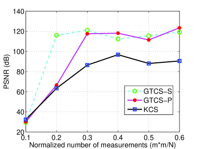
(a) PSNR comparison

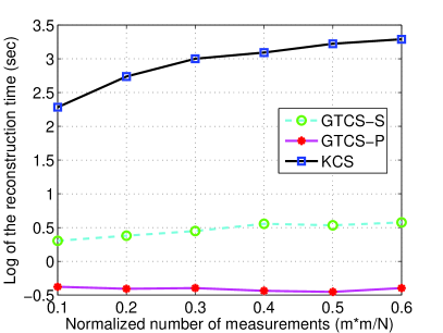
(b) Recovery time comparison

Figure 2: Performance comparison among the tested methods in terms of PSNR and reconstruction time in the scenario of noiseless recovery of a sparse image.

2.3 Recovery of Data in the Presence of Noise

Consider the case where the observation is noisy. For a given integer $k$, a matrix $A\in\mathbb{R}^{m\times N}$ satisfies the restricted isometry property (RIP_k) RIP if

$$(1-\delta_{k})\|x\|^{2}_{2}\leq\|Ax\|^{2}_{2}\leq(1+\delta_{k})\|x\|^{2}_{2}$$

for all $x\in\Sigma_{k,N}$ and for some $\delta_{k}\in(0,1)$.

It was shown in C2 that the reconstruction in the presence of noise is achieved by solving

$$\hat{x}=\arg\min_{z}\|z\|_{1},\quad\text{s.t.}\quad\|Az-y\|_{2}\leq\varepsilon,$$ (12)

which has complexity $O(N^{3})$.

Lemma 2

Assume that $A\in\mathbb{R}^{m\times N}$ satisfies the RIP_2k property for some $\delta_{2k}\in(0,\sqrt{2}-1)$. Let $x\in\Sigma_{k,N},y=Ax+e,$ where $e$ denotes the noise vector, and $\|e\|_{2}\leq\varepsilon$ for some real nonnegative number $\varepsilon$. Then

$$\|\hat{x}-x\|_{2}\leq C_{2}\varepsilon,\textrm{ where }C_{2}=\frac{4\sqrt{1+\delta_{2k}}}{1-(1+\sqrt{2})\delta_{2k}}.$$ (13)

Compressed Sensing of Matrices - Serial Recovery (CSM-S) in the Presence of Noise

The serial recovery method for compressed sensing of matrices in the presence of noise is described by the following theorem.

Theorem 2.3 (CSM-S in the presence of noise)

Let $X=[x_{ij}]\in\mathbb{R}^{N_{1}\times N_{2}}$ be $k$-sparse. Let $U_{i}\in\mathbb{R}^{m_{i}\times N_{i}}$ and assume that $U_{i}$ satisfies the RIP_2k property for some $\delta_{2k}\in(0,\sqrt{2}-1)$, $i\in[2]$. Define

$$Y=[y_{pq}]=U_{1}XU_{2}^{T}+E,\quad Y\in\mathbb{R}^{m_{1}\times m_{2}},$$ (14)

where $E$ denotes the noise matrix, and $\|E\|_{F}\leq\epsilon$ for some real nonnegative number $\epsilon$. Then $X$ can be recovered approximately as follows. Let $c_{1}(Y),\ldots,c_{m_{2}}(Y)\in\mathbb{R}^{m_{1}}$ denote the columns of $Y$. Let $\hat{z}_{i}\in\mathbb{R}^{N_{1}}$ be a solution of

$$\hat{z}_{i}=\arg\min_{z_{i}}\|z_{i}\|_{1}\quad\text{s.t.}\quad\|c_{i}(Y)-U_{1}z_{i}\|_{2}\leq\epsilon,\quad i\in[m_{2}].$$ (15)

Let $Z\in\mathbb{R}^{N_{1}\times m_{2}}$ be the matrix whose columns are $\hat{z}_{1},\ldots,\hat{z}_{m_{2}}$. According to Eq. (13), $\|c_{i}(Z)-c_{i}(XU_{2}^{T})\|_{2}=\|\hat{z}_{i}-c_{i}(XU_{2}^{T})\|_{2}\leq C_{2}\varepsilon$, hence $\|Z-XU_{2}^{T}\|_{F}\leq\sqrt{m_{2}}C_{2}\varepsilon$. Let $c_{1}(Z^{T}),\ldots,c_{N_{1}}(Z^{T})$ be the rows of $Z$. Then $u_{j}\in\mathbb{R}^{N_{2}}$, the $j$-th row of $X$, is the solution of

$$\hat{u}_{j}=\arg\min_{u_{j}}\|u_{j}\|_{1}\quad\text{s.t.}\quad\|c_{j}(Z^{T})-U_{2}u_{j}\|_{2}\leq\sqrt{m_{2}}C_{2}\varepsilon,\quad j\in[N_{1}].$$ (16)

Denote by $\hat{X}$ the recovered matrix, then according to Eq. (13),

$$\|\hat{X}-X\|_{F}\leq\sqrt{m_{2}N_{1}}C_{2}^{2}\varepsilon.$$ (17)

Proof

The proof of the theorem follows from Lemma 2. ∎

The upper bound in Eq. (17) can be tightened by assuming that the entries of $E$ adhere to a specific type of distribution. Let $E=[e_{1},\ldots,e_{m_{2}}]$. Suppose that each entry of $E$ is an independent random variable with a given distribution having zero mean. Then we can assume that $\|e_{j}\|_{2}\leq\frac{\varepsilon}{\sqrt{m_{2}}}$, which implies that $\|E\|_{F}\leq\varepsilon$.

Each $z_{i}$ can be recovered by finding a solution to

$$\hat{z}_{i}=\arg\min_{z_{i}}\|z_{i}\|_{1}\quad\text{s.t.}\quad\|c_{i}(Y)-U_{1}z_{i}\|_{2}\leq\frac{\varepsilon}{\sqrt{m_{2}}},\quad i\in[m_{2}].$$ (18)

Let $Z=[\hat{z}_{1}\ldots\hat{z}_{m_{2}}]\in\mathbb{R}^{N_{1}\times m_{2}}$. According to Eq. (13), $\|c_{i}(Z)-c_{i}(XU_{2}^{T})\|_{2}=\|\hat{z}_{i}-c_{i}(XU_{2}^{T})\|_{2}\leq C_{2}\frac{\varepsilon}{\sqrt{m_{2}}}$; therefore $\|Z-XU_{2}^{T}\|_{F}\leq C_{2}\varepsilon$.

Let $E_{1}:=Z-XU_{2}^{T}$ be the error matrix, and assume that the entries of $E_{1}$ adhere to the same distribution as the entries of $E$. Hence, $\|c_{i}(Z^{T})-c_{i}(U_{2}X^{T})\|_{2}\leq\frac{C_{2}\varepsilon}{\sqrt{N_{1}}}$.

$\hat{X}$ can be reconstructed by recovering each row of $X$:

$$\hat{u}_{j}=\arg\min_{u_{j}}\|u_{j}\|_{1}\quad\text{s.t.}\quad\|c_{j}(Z^{T})-U_{2}u_{j}\|_{2}\leq\frac{C_{2}\varepsilon}{\sqrt{N_{1}}},\quad j\in[N_{1}].$$ (19)

Consequently, $\|\hat{u}_{j}-c_{j}(X^{T})\|_{2}\leq\frac{C_{2}^{2}\varepsilon}{\sqrt{N_{1}}}$, and the recovery error is bounded as follows:

$$\|\hat{X}-X\|_{F}\leq C_{2}^{2}\varepsilon.$$ (20)

When $Y$ is not full-rank, the above procedure is equivalent to the following alternative. Let $Y_{k}$ be a best rank-$k$ approximation of $Y$:

$$Y_{k}=\sum_{i=1}^{k}(\sqrt{\tilde{\sigma}_{i}}\tilde{u}_{i})(\sqrt{\tilde{\sigma}_{i}}\tilde{v}_{i})^{T}.$$ (21)

Here, $\tilde{\sigma}_{i}$ is the $i$-th singular value of $Y$, and $\tilde{u}_{i},\tilde{v}_{i}$ are the corresponding left and right singular vectors of $Y$ for $i\in[k]$, assume that $k\leq\min(m_{1},m_{2})$. Since $X$ is assumed to be $k$-sparse, then $\mathrm{rank\;}(X)\leq k$. Hence the ranks of $XU_{2}$ and $U_{1}XU_{2}^{T}$ are less than or equal to $k$. In this case, recovering $X$ amounts to following the procedure described above with $Y_{k}$ and $Z_{k}$ taking the place of $Y$ and $Z$ respectively.

Compressed Sensing of Matrices - Parallelizable Recovery (CSM-P) in the Presence of Noise

The parallelizable recovery method for compressed sensing of matrices in the presence of noise is described by the following theorem.

Theorem 2.4 (CSM-P in the presence of noise)

Let $X=[x_{ij}]\in\mathbb{R}^{N_{1}\times N_{2}}$ be $k$-sparse. Let $U_{i}\in\mathbb{R}^{m_{i}\times N_{i}}$ and assume that $U_{i}$ satisfies the RIP_2k property for some $\delta_{2k}\in(0,\sqrt{2}-1)$, $i\in[2]$. Let $Y$ be as defined in Eq. (14). Then $X$ can be recovered uniquely as follows. Let $Y_{k^{\prime}}$ be a best rank-$k^{\prime}$ approximation of $Y$ as in Eq. (21), where $k^{\prime}$ is the minimum of $k$ and the number of singular values of $Y$ greater than $\frac{\varepsilon}{\sqrt{k}}$. Then $\hat{X}=\sum_{i=1}^{k^{\prime}}\frac{1}{\tilde{\sigma}_{i}}\hat{x}_{i}{\hat{y}_{i}}^{T}$ and

$$\|X-\hat{X}\|_{F}\leq C^{2}\varepsilon,$$ (22)

where

$$\hat{x}_{i}=\arg\min_{x_{i}}\|x_{i}\|_{1}\quad\text{s.t.}\quad\|\tilde{\sigma}_{i}\tilde{u}_{i}-U_{1}x_{i}\|_{2}\leq\frac{\varepsilon}{\sqrt{2k}},$$

$$\hat{y}_{i}=\arg\min_{y_{i}}\|y_{i}\|_{1}\quad\text{s.t.}\quad\|\tilde{\sigma}_{i}\tilde{v}_{i}-U_{2}y_{i}\|_{2}\leq\frac{\varepsilon}{\sqrt{2k}},$$ (23)

$$i\in[k].$$

Proof

Assume that $k<\min(m_{1},m_{2})$, otherwise $Y_{k}=Y$. Since $\mathrm{rank\;}(U_{1}XU_{2})\leq k$, $Y_{k}=U_{1}XU_{2}+E_{k}$. Let

$$U_{1}XU_{2}^{T}=\sum_{i=1}^{k}(\sqrt{\sigma_{i}}u_{i})(\sqrt{\sigma_{i}}v_{i})^{T}$$ (24)

be the SVD of $U_{1}XU_{2}^{T}$. Then $\|u_{i}\|=\|\tilde{u}_{i}\|=\|v_{i}\|=\|\tilde{v}_{i}\|=1$ for $i\in[k]$.

Assuming

$$e_{i}:=\sqrt{\tilde{\sigma}_{i}}\tilde{u}_{i}-\sqrt{\sigma_{i}}u_{i},\quad f_{i}:=\sqrt{\tilde{\sigma}_{i}}\tilde{v}_{i}-\sqrt{\sigma_{i}}v_{i},\quad i\in[k],$$ (25)

then the entries of $e_{i}$ and $f_{i}$ are independent Gaussian variables with zero mean and standard deviation $\frac{\varepsilon}{\sqrt{2\sigma_{i}m_{1}k}}$ and $\frac{\varepsilon}{\sqrt{2\sigma_{i}m_{2}k}}$, respectively, for $i\in[k]$. When $\varepsilon^{2}\ll\varepsilon$,

$$E_{k}\approx\sum_{i=1}^{k}e_{i}(\sqrt{\sigma_{i}}v_{i}^{T})+\sum_{i=1}^{k}(\sqrt{\sigma_{i}}u_{i})f_{i}^{T}.$$ (26)

In this scenario,

$$\|\sqrt{\sigma_{i}}u_{i}-\sqrt{\tilde{\sigma}_{i}}\tilde{u}_{i}\|\leq\frac{\varepsilon}{\sqrt{2k\sigma_{i}}},\quad\|\sqrt{\sigma_{i}}v_{i}-\sqrt{\tilde{\sigma}_{i}}\tilde{v}_{i}\|\leq\frac{\varepsilon}{\sqrt{2k\sigma_{i}}}.$$ (27)

Note that

$$\sum_{i=1}^{\min(m_{1},m_{2})}(\sigma_{i}-\sigma(Y_{k}))^{2}\leq\mathop{\mathrm{tr}}\nolimits(EE^{T})\leq\varepsilon^{2},\quad\sum_{i=1}^{k}(\sigma_{i}-\tilde{\sigma}_{i})^{2}\leq\mathop{\mathrm{tr}}\nolimits(E_{k}E_{k}^{T})\leq\varepsilon^{2}.$$ (28)

Given the way $k^{\prime}$ is defined, it can be interpreted as the numerical rank of $Y$. Consequently, $Y$ can be well represented by its best rank $k^{\prime}$ approximation. Thus

$$U_{1}XU_{2}^{T}\approx\sum_{i=1}^{k^{\prime}}(\sqrt{\sigma_{i}}u_{i})(\sqrt{\sigma_{i}}v_{i}^{T}),\quad Y_{k^{\prime}}=\sum_{i=1}^{k^{\prime}}(\sqrt{\tilde{\sigma}_{i}}\tilde{u}_{i})(\sqrt{\tilde{\sigma}_{i}}\tilde{v}_{i}^{T}),\quad i\in[k^{\prime}].$$ (29)

Assuming $\sigma_{i}\approx\tilde{\sigma}_{i}$ for $i\in[k^{\prime}]$, we conclude that

$$\|\tilde{\sigma}_{i}\tilde{u}_{i}-\sigma_{i}u_{i}\|\leq\frac{\varepsilon}{\sqrt{2k}},\quad\|\tilde{\sigma}_{i}\tilde{v}_{i}-\sigma_{i}v_{i}\|\leq\frac{\varepsilon}{\sqrt{2k}}.$$ (30)

A compressed sensing framework can be used to solve the following set of minimization problems, for $i\in[k^{\prime}]$:

$$\hat{x}_{i}=\arg\min_{x_{i}}\|x_{i}\|_{1}\quad\text{s.t.}\quad\|\tilde{\sigma}_{i}\tilde{u}_{i}-U_{1}x_{i}\|_{2}\leq\frac{\varepsilon}{\sqrt{2k}},$$ (31)

$$\hat{y}_{i}=\arg\min_{y_{i}}\|y_{i}\|_{1}\quad\text{s.t.}\quad\|\tilde{\sigma}_{i}\tilde{v}_{i}-U_{2}y_{i}\|_{2}\leq\frac{\varepsilon}{\sqrt{2k}}.$$ (32)

The error bound from Eq. (22) follows. ∎

Simulation Results

In this section, we use the same target image and experimental settings used in Section 2.2. We simulate the noisy recovery scenario by modifying the observation with additive, zero-mean Gaussian noise having standard deviation values ranging from 1 to 10 in steps of 1, and attempt to recover the target image using Eq. (12). As before, reconstruction performance is measured in terms of PSNR between the recovered and the target image, and in terms of reconstruction time, as illustrated in Figs. 3 and 4.

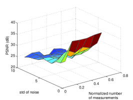
(a) GTCS-S

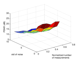
(b) GTCS-P

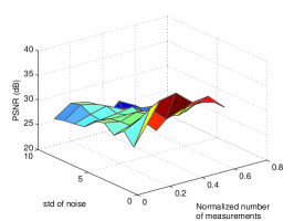
(c) KCS

Figure 3: PSNR between target and recovered image for the tested methods in the noisy recovery scenario.

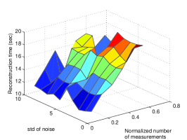
(a) GTCS-S

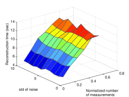
(b) GTCS-P

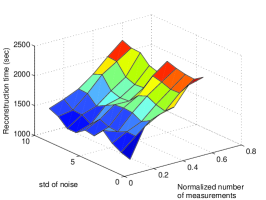
(c) KCS

Figure 4: Execution time for the tested methods in the noisy recovery scenario.

3 Compressed Sensing of Tensors

3.1 A Brief Introduction to Tensors

A tensor is a multidimensional array. The order of a tensor is the number of modes. For instance, tensor $\mathcal{X}\in\mathbb{R}^{N_{1}\times\ldots\times N_{d}}$ has order $d$ and the dimension of its $i^{th}$ mode (denoted mode $i$) is $N_{i}$.

Definition 1 (Kronecker Product)

The Kronecker product between matrices $A\in\mathbb{R}^{I\times J}$ and $B\in\mathbb{R}^{K\times L}$ is denoted by $A\otimes B$. The result is the matrix of dimensions $(I\cdot K)\times(J\cdot L)$ defined by

$A\otimes B=\left(\begin{array}[]{cccc}a_{11}B&a_{12}B&\cdots&a_{1J}B\\ a_{21}B&a_{22}B&\cdots&a_{2J}B\\ \vdots&\vdots&\ddots&\vdots\\ a_{I1}B&a_{I2}B&\cdots&a_{IJ}B\\ \end{array}\right)$.

Definition 2 (Outer Product and Tensor Product)

The operator $\circ$ denotes the tensor product between two vectors. In linear algebra, the outer product typically refers to the tensor product between two vectors, that is, $u\circ v=uv^{T}$. In this chapter, the terms outer product and tensor product are equivalent. The Kronecker product and the tensor product between two vectors are related by $u\circ v=u\otimes v^{T}.$

Definition 3 (Mode-$i$ Product)

The mode-$i$ product of a tensor $\mathcal{X}=[x_{\alpha_{1},\ldots,\alpha_{d}}]\in\mathbb{R}^{N_{1}\times\ldots\times N_{d}}$ and a matrix $U=[u_{j,\alpha_{i}}]\in\mathbb{R}^{J\times N_{i}}$ is denoted by $\mathcal{X}\times_{i}U$ and is of size $N_{1}\times\ldots\times N_{i-1}\times J\times N_{i+1}\times\ldots\times N_{d}$. Element-wise, the mode-$i$ product can be written as $(\mathcal{X}\times_{i}U)_{\alpha_{1},\ldots,\alpha_{i-1},j,\alpha_{i+1},\ldots,\alpha_{d}}=\sum_{\alpha_{i}=1}^{N_{i}}x_{\alpha_{1},\ldots,\alpha_{d}}u_{j,\alpha_{i}}$.

Definition 4 (Mode-$i$ Fiber and Mode-$i$ Unfolding)

The mode-$i$ fiber of tensor $\mathcal{X}=[x_{\alpha_{1},\ldots,\alpha_{d}}]\in\mathbb{R}^{N_{1}\times\ldots\times N_{d}}$ is the set of vectors obtained by fixing every index but $\alpha_{i}$. The mode-$i$ unfolding $X_{(i)}$ of $\mathcal{X}$ is the $N_{i}\times(N_{1}\cdot\ldots\cdot N_{i-1}\cdot N_{i+1}\cdot\ldots\cdot N_{d})$ matrix whose columns are the mode-$i$ fibers of $\mathcal{X}$. $\mathcal{Y}=\mathcal{X}\times_{1}U_{1}\times\ldots\times_{d}U_{d}$ is equivalent to $Y_{(i)}=U_{i}X_{(i)}(U_{d}\otimes\ldots\otimes U_{i+1}\otimes U_{i-1}\otimes\ldots\otimes U_{1})^{T}$.

Definition 5 (Core Tucker Decomposition)

Tuck1964 Let $\mathcal{X}\in\mathbb{R}^{N_{1}\times\ldots\times N_{d}}$ be a tensor with mode-$i$ unfolding $X_{(i)}\in\mathbb{R}^{N_{i}\times(N_{1}\cdot\ldots\cdot N_{i-1}\cdot N_{i+1}\cdot\ldots\cdot N_{d})}$ such that $\mathrm{rank\;}(X_{(i)})=r_{i}$. Let $R_{i}(\mathcal{X})\subset\mathbb{R}^{N_{i}}$ denote the column space of $X_{(i)}$, and $c_{1,i},\ldots,c_{r_{i},i}$ be a basis in $R_{i}(\mathcal{X})$. Then $\mathcal{X}$ is an element of the subspace $\mathbf{V}(\mathcal{X}):=R_{1}(\mathcal{X})\circ\ldots\circ R_{d}(\mathcal{X})\subset\mathbb{R}^{N_{1}\times\ldots\times N_{d}}$. Clearly, vectors $c_{i_{1},1}\circ\ldots\circ c_{i_{d},d}$, where $i_{j}\in[r_{j}]$ and $j\in[d]$, form a basis of $\mathbf{V}$. The core Tucker decomposition of $\mathcal{X}$ is

$$\mathcal{X}=\sum_{i_{j}\in[r_{j}],j\in[d]}\xi_{i_{1},\ldots,i_{d}}c_{i_{1},1}\circ\ldots\circ c_{i_{d},d}$$ (33)

for some decomposition coefficients $\xi_{i_{1},\ldots,i_{d}}$, $i_{j}\in[r_{j}]$ and $j\in[d]$.

A special case of the core Tucker decomposition is the higher-order singular value decomposition (HOSVD). Any tensor $\mathcal{X}\in\mathbb{R}^{N_{1}\times\ldots\times N_{d}}$ can be written as

$$\mathcal{X}=\mathcal{S}\times_{1}U_{1}\times\ldots\times_{d}U_{d},$$ (34)

where $U_{i}=[u_{1}\cdots u_{N_{i}}]$ is an orthonormal matrix for $i\in[d]$, and $\mathcal{S}=\mathcal{X}\times_{1}U_{1}^{T}\times\ldots\times_{d}U_{d}^{T}$ is called the core tensor. For a more in-depth discussion on HOSVD, including the set of properties the core tensor is required to satisfy, please refer to HOSVD .

$\mathcal{X}$ can also be expressed in terms of weaker decompositions of the form

$$\mathcal{X}=\sum_{i=1}^{K}a_{i}^{(1)}\circ\ldots\circ a_{i}^{(d)},\quad a_{i}^{(j)}\in R_{j}(\mathcal{X}),j\in[d].$$ (35)

For instance, first decompose $X_{(1)}$ as $X_{(1)}=\sum_{j=1}^{r_{1}}c_{j,1}g_{j,1}^{T}$ (e.g., via SVD); then each $g_{j,1}$ can be viewed as a tensor of order $d-1$ $\in R_{2}(\mathcal{X})\circ\ldots\circ R_{d}(\mathcal{X})\subset\mathbb{R}^{N_{2}\times\ldots\times N_{d}}$. Secondly, unfold each $g_{j,1}$ in mode $2$ to obtain ${g_{j,1}}_{(2)}$ and decompose ${g_{j,1}}_{(2)}=\sum_{l=1}^{r_{2}}d_{l,2,j}f_{l,2,j}^{T},\quad d_{l,2,j}\in R_{2}(\mathcal{X}),f_{l,2,j}\in R_{3}(\mathcal{X})\circ\ldots\circ R_{d}(\mathcal{X}).$ By successively unfolding and decomposing each remaining tensor mode, a decomposition of the form in Eq. (35) is obtained. Note that if $\mathcal{X}$ is $k$-sparse, then each vector in $R_{i}(\mathcal{X})$ is $k$-sparse and $r_{i}\leq k$ for $i\in[d]$. Hence, $K\leq k^{d-1}$.

Definition 6 (CANDECOMP/PARAFAC Decomposition)

Kolda09tensordecompositions For a tensor $\mathcal{X}\in\mathbb{R}^{N_{1}\times\ldots\times N_{d}}$, the CANDECOMP/PARAFAC (CP) decomposition is defined as $\mathcal{X}\approx[\lambda;A^{(1)},\ldots,A^{(d)}]\equiv\sum_{r=1}^{R}\lambda_{r}a_{r}^{(1)}\circ\ldots\circ a_{r}^{(d)},$ where $\lambda=[\lambda_{1}\ldots\lambda_{R}]^{T}\in\mathbb{R}^{R}$ and $A^{(i)}=[a_{1}^{(i)}\cdots a_{R}^{(i)}]\in\mathbb{R}^{N_{i}\times R}$ for $i\in[d].$

3.2 Noiseless Recovery

Generalized Tensor Compressed Sensing - Serial Recovery (GTCS-S)

The serial recovery method for compressed sensing of tensors in the noiseless case is described by the following theorem.

Theorem 3.1

Let $\mathcal{X}=[x_{i_{1},\ldots,i_{d}}]\in\mathbb{R}^{N_{1}\times\ldots\times N_{d}}$ be $k$-sparse. Let $U_{i}\in\mathbb{R}^{m_{i}\times N_{i}}$ and assume that $U_{i}$ satisfies the NSP_k property for $i\in[d]$. Define

$$\mathcal{Y}=[y_{j_{1},\ldots,j_{d}}]=\mathcal{X}\times_{1}U_{1}\times\ldots\times_{d}U_{d}\in\mathbb{R}^{m_{1}\times\ldots\times m_{d}}.$$ (36)

Then $\mathcal{X}$ can be recovered uniquely as follows. Unfold $\mathcal{Y}$ in mode $1$,

$$Y_{(1)}=U_{1}X_{(1)}[\otimes_{k=d}^{2}U_{k}]^{T}\in\mathbb{R}^{m_{1}\times(m_{2}\cdot\ldots\cdot m_{d})}.$$

Let $y_{1},\ldots,y_{m_{2}\cdot\ldots\cdot m_{d}}$ be the columns of $Y_{(1)}$. Then $y_{i}=U_{1}z_{i}$, where each $z_{i}\in\mathbb{R}^{N_{1}}$ is $k$-sparse. Recover each $z_{i}$ using Eq. (1). Let $\mathcal{Z}=\mathcal{X}\times_{2}U_{2}\times\ldots\times_{d}U_{d}\in\mathbb{R}^{N_{1}\times m_{2}\times\ldots\times m_{d}}$, and let $z_{1},\ldots,z_{m_{2}\cdot\ldots\cdot m_{d}}$ denote its mode-$1$ fibers. Unfold $\mathcal{Z}$ in mode 2,

$$Z_{(2)}=U_{2}X_{(2)}[\otimes_{k=d}^{3}U_{k}\otimes I]^{T}\in\mathbb{R}^{m_{2}\times(N_{1}\cdot m_{3}\cdot\ldots\cdot m_{d})}.$$

Let $w_{1},\ldots,w_{N_{1}\cdot m_{3}\cdot\ldots\cdot m_{d}}$ be the columns of $Z_{(2)}$. Then $w_{j}=U_{2}v_{j}$, where each $v_{j}\in\mathbb{R}^{N_{2}}$ is $k$-sparse. Recover each $v_{j}$ using Eq. (1). $\mathcal{X}$ can be reconstructed by successively applying the above procedure to tensor modes $3,\ldots,d$.

Proof

The proof of this theorem is a straightforward generalization of that of Theorem 2.1.∎

Note that although Theorem 3.1 requires $U_{i}$ to satisfy the NSP_k property for $i\in[d]$, such constraints can be relaxed if each mode-$i$ fiber of $\mathcal{X}\times_{i+1}U_{i+1}\times\ldots\times_{d}U_{d}$ is $k_{i}$-sparse for $i\in[d-1]$, and each mode-$d$ fiber of $\mathcal{X}$ is $k_{d}$-sparse, where $k_{i}\leq k$, for $i\in[d]$. In this case, it follows from the proof of Theorem 3.1 that $X$ can be recovered as long as $U_{i}$ satisfies the NSP${}_{k_{i}}$ property, for $i\in[d]$.

Generalized Tensor Compressed Sensing - Parallelizable Recovery (GTCS-P)

The parallelizable recovery method for compressed sensing of tensors in the noiseless case is described by the following theorem.

Theorem 3.2 (GTCS-P)

Let $\mathcal{X}=[x_{i_{1},\ldots,i_{d}}]\in\mathbb{R}^{N_{1}\times\ldots\times N_{d}}$ be $k$-sparse. Let $U_{i}\in\mathbb{R}^{m_{i}\times N_{i}}$ and assume that $U_{i}$ satisfies the NSP_k property for $i\in[d]$. If $\mathcal{Y}$ is given by Eq. (36), then $\mathcal{X}$ can be recovered uniquely as follows. Consider a decomposition of $\mathcal{Y}$ such that,

$$\mathcal{Y}=\sum_{i=1}^{K}b_{i}^{(1)}\circ\ldots\circ b_{i}^{(d)},\quad b_{i}^{(j)}\in R_{j}(\mathcal{Y})\subseteq U_{j}R_{j}(\mathcal{X}),j\in[d].$$ (37)

Let $\hat{w}_{i}^{(j)}\in R_{j}(\mathcal{X})\subset\mathbb{R}^{N_{j}}$ be a solution of

$$\hat{w}_{i}^{(j)}=\arg\min_{w_{i}^{(j)}}\|w_{i}^{(j)}\|_{1}\quad\text{s.t.}\quad b_{i}^{(j)}=U_{j}w_{i}^{(j)},\quad i\in[K],j\in[d].$$ (38)

Thus each $\hat{w}_{i}^{(j)}$ is unique and $k$-sparse. Then,

$$\mathcal{X}=\sum_{i=1}^{K}w_{i}^{(1)}\circ\ldots\circ w_{i}^{(d)},\quad w_{i}^{(j)}\in R_{j}(\mathcal{X}),j\in[d].$$ (39)

Proof

Since $\mathcal{X}$ is $k$-sparse, each vector in $R_{j}(\mathcal{X})$ is $k$-sparse. If each $U_{j}$ satisfies the NSP_k property, then $w_{i}^{(j)}\in R_{j}(\mathcal{X})$ is unique and $k$-sparse. Define $\mathcal{Z}$ as

$$\mathcal{Z}=\sum_{i=1}^{K}w_{i}^{(1)}\circ\ldots\circ w_{i}^{(d)},\quad w_{i}^{(j)}\in R_{j}(\mathcal{X}),j\in[d].$$ (40)

Then

$$(\mathcal{X}-\mathcal{Z})\times_{1}U_{1}\times\ldots\times_{d}U_{d}=0.$$ (41)

To show $\mathcal{Z}=\mathcal{X}$, assume a slightly more general scenario, where each $R_{j}(\mathcal{X})\subseteq\mathbf{V}_{j}\subset\mathbb{R}^{N_{j}}$, such that each nonzero vector in $\mathbf{V}_{j}$ is $k$-sparse. Then $R_{j}(\mathcal{Y})\subseteq U_{j}R_{j}(\mathcal{X})\subseteq U_{j}\mathbf{V}_{j}$ for $j\in[d]$. Assume to the contrary that $\mathcal{X}\neq\mathcal{Z}$. This hypothesis can be disproven via induction on mode $m$ as follows.

Suppose

$$(\mathcal{X}-\mathcal{Z})\times_{m}U_{m}\times\ldots\times_{d}U_{d}=0.$$ (42)

Unfold $\mathcal{X}$ and $\mathcal{Z}$ in mode $m$, then the column (row) spaces of $X_{(m)}$ and $Z_{(m)}$ are contained in $\mathbf{V}_{m}$ ($\hat{\mathbf{V}}_{m}:=\mathbf{V}_{1}\circ\ldots\circ\mathbf{V}_{m-1}\circ\mathbf{V}_{m+1}\circ\ldots\circ\mathbf{V}_{d}$). Since $\mathcal{X}\neq\mathcal{Z}$, $X_{(m)}-Z_{(m)}\neq 0$. Then $X_{(m)}-Z_{(m)}=\sum_{i=1}^{p}u_{i}v_{i}^{T}$, where $\mathrm{rank\;}(X_{(m)}-Z_{(m)})=p$, and $u_{1},\ldots,u_{p}\in\mathbf{V}_{m},v_{1},\ldots,v_{p}\in\hat{\mathbf{V}}_{m}$ are two sets of linearly independent vectors.

Since $(\mathcal{X}-\mathcal{Z})\times_{m}U_{m}\times\ldots\times_{d}U_{d}=0$,

$$0 =U_{m}(X_{(m)}-Z_{(m)})(U_{d}\otimes\ldots\otimes U_{m+1}\otimes I)^{T}$$

$$=U_{m}(X_{(m)}-Z_{(m)})\hat{U}_{m}^{T}$$

$$=\sum_{i=1}^{p}(U_{m}u_{i})(\hat{U}_{m}v_{i})^{T}.$$

Since $U_{m}u_{1},\ldots,U_{m}u_{p}$ are linearly independent (see Appendix for proof), it follows that $\hat{U}_{m}v_{i}=0$ for $i\in[p]$. Therefore,

$$(X_{(m)}-Z_{(m)})\hat{U}_{m}^{T}=(\sum_{i=1}^{p}u_{i}v_{i}^{T})\hat{U}_{m}^{T}=\sum_{i=1}^{p}u_{i}(\hat{U}_{m}v_{i})^{T}=0,$$

which is equivalent to (in tensor form, after folding)

$$(\mathcal{X}-\mathcal{Z})\times_{m}I_{m}\times_{m+1}U_{m+1}\times\ldots\times_{d}U_{d}$$

$$=(\mathcal{X}-\mathcal{Z})\times_{m+1}U_{m+1}\times\ldots\times_{d}U_{d}=0,$$ (43)

where $I_{m}$ is the $N_{m}\times N_{m}$ identity matrix. Note that Eq. (42) leads to Eq. (3.2) upon replacing $U_{m}$ with $I_{m}$. Similarly, when $m=1$, $U_{1}$ can be replaced with $I_{1}$ in Eq. (41). By successively replacing $U_{m}$ with $I_{m}$ for $2\leq m\leq d$,

$$(\mathcal{X}-\mathcal{Z})\times_{1}U_{1}\times\ldots\times_{d}U_{d}$$

$$= (\mathcal{X}-\mathcal{Z})\times_{1}I_{1}\times\ldots\times_{d}I_{d}$$

$$= \mathcal{X}-\mathcal{Z}=0,$$

which contradicts the assumption that $\mathcal{X}\neq\mathcal{Z}$. Thus, $\mathcal{X}=\mathcal{Z}$. This completes the proof. ∎

Note that although Theorem 3.2 requires $U_{i}$ to satisfy the NSP_k property for $i\in[d]$, such constraints can be relaxed if all vectors $\in R_{i}(\mathcal{X})$ are $k_{i}$-sparse. In this case, it follows from the proof of Theorem 3.2 that $X$ can be recovered as long as $U_{i}$ satisfies the NSP${}_{k_{i}}$, for $i\in[d]$.

As in the matrix case, the reconstruction stage of the recovery process can be implemented in parallel for each tensor mode.

Note additionally that Theorem 3.2 does not require tensor rank decomposition, which is an NP-hard problem. Weaker decompositions such as the one described by Eq. 35 can be utilized.

The above described procedure allows exact recovery. In some cases, recovery of a rank-$R$ approximation of $\mathcal{X}$, $\mathcal{\hat{X}}=\sum_{r=1}^{R}w_{r}^{(1)}\circ\ldots\circ w_{r}^{(d)}$, suffices. In such scenarios, $\mathcal{Y}$ in Eq. (37) can be replaced by its rank-$R$ approximation, namely, $\mathcal{Y}=\sum_{r=1}^{R}b_{r}^{(1)}\circ\ldots\circ b_{r}^{(d)}$ (obtained e.g.,  by CP decomposition).

Simulation Results

Examples of data that is amendable to tensorial representation include color and multi-spectral images and video. We use a 24-frame, $24\times 24$ pixel grayscale video to test the performance of our algorithm (see Fig. 5). In other words, the video data is represented as a $24\times 24\times 24$ tensor ($N=13824$). We use the three-dimensional DCT as the sparsifying transform, and zero-out coefficients outside the $6\times 6\times 6$ cube located on the front upper left corner of the transformed tensor. As in the image case, let $m$ denote the number of measurements along each tensor mode; we generate the measurement matrices with entries drawn from a Gaussian distribution with mean $0$ and standard deviation $\sqrt{\frac{1}{m}}$. For simplicity, we set the number of measurements for each tensor mode to be equal; that is, the randomly constructed Gaussian matrix $U$ is of size $m\times 24$ for each mode. Therefore, the KCS measurement matrix $U\otimes U\otimes U$ is of size $m^{3}\times 13824$, and the total number of measurements is $m^{3}$. We refer to $\frac{m^{3}}{N}$ as the normalized number of measurements. For GTCS-P, we employ the weaker form of the core Tucker decomposition as described in Section 3.1. Although the reconstruction stage of GTCS-P is parallelizable, we recover each vector in series. We examine the performance of KCS and GTCS-P by varying the normalized number of measurements from 0.1 to 0.6 in steps of 0.1. Reconstruction accuracy is measured in terms of the average PSNR across all frames between the recovered and the target video, whereas computational complexity is measured in terms of the $\log$ of the reconstruction time (see Fig. 6).

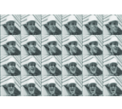
Figure 5: The original 24 video frames.

Note that in the tensor case, due to the serial nature of GTCS-S, the reconstruction error propagates through the different stages of the recovery process. Since exact reconstruction is rarely achieved in practice, the equality constraint in the $\ell_{1}$-minimization process described by Eq. (1) becomes increasingly difficult to satisfy for the latter stages of the reconstruction process. In this case, a relaxed recovery procedure as described in Eq. (12) can be employed. Since the relaxed constraint from Eq. (12) results in what effectively amounts to recovery in the presence of noise, we do not compare the performance of GTCS-S with that of the other two methods.

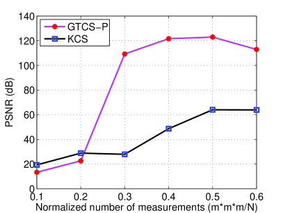
(a) PSNR comparison

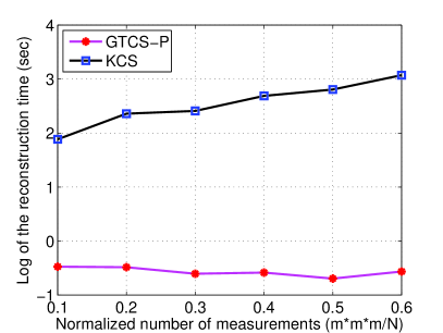
(b) Recovery time comparison

Figure 6: Performance comparison among the tested methods in terms of PSNR and reconstruction time in the scenario of noiseless recovery of the sparse video.

3.3 Recovery in the Presence of Noise

Generalized Tensor Compressed Sensing - Serial Recovery (GTCS-S) in the Presence of Noise

Let $\mathcal{X}=[x_{i_{1},\ldots,i_{d}}]\in\mathbb{R}^{N_{1}\times\ldots\times N_{d}}$ be $k$-sparse. Let $U_{i}\in\mathbb{R}^{m_{i}\times N_{i}}$ and assume that $U_{i}$ satisfies the NSP_k property for $i\in[d]$. Define

$$\mathcal{Y}=[y_{j_{1},\ldots,j_{d}}]=\mathcal{X}\times_{1}U_{1}\times\ldots\times_{d}U_{d}+\mathcal{E}\in\mathbb{R}^{m_{1}\times\ldots\times m_{d}},$$ (44)

where $\mathcal{E}$ is the noise tensor and $\|\mathcal{E}\|_{F}\leq\varepsilon$ for some real nonnegative number $\epsilon$. Although the norm of the noise tensor is not equal across different stages of GTCS-S, it is assumed that at any given stage, the entries of the error tensor are independent and identically distributed. The upper bound of the reconstruction error for GTCS-S recovery in the presence of noise is derived next by induction on mode $k$.

When $k=1$, unfold $\mathcal{Y}$ in mode $1$ to obtain matrix $Y_{(1)}\in\mathbb{R}^{m_{1}\times(m_{2}\cdot\ldots\cdot m_{d})}$. Recover each $z_{i}^{(1)}$ by

$$\hat{z}_{i}^{(1)}=\arg\min_{z_{i}^{(1)}}\|z_{i}^{(1)}\|_{1}\quad\text{s.t.}\quad\|c_{i}(Y_{(1)})-U_{1}z_{i}^{(1)}\|_{2}\leq\frac{\varepsilon}{\sqrt{m_{2}\cdot\ldots\cdot m_{d}}}.$$ (45)

Let $\hat{Z}^{(1)}=[\hat{z}_{1}^{(1)}\ldots\hat{z}_{m_{2}\cdot\ldots\cdot m_{d}}^{(1)}]\in\mathbb{R}^{N_{1}\times(m_{2}\cdot\ldots\cdot m_{d})}$. According to Eq. (13), $\|\hat{z}_{i}^{(1)}-c_{i}(X_{(1)}[\otimes_{k=d}^{2}U_{k}]^{T})\|_{2}\leq C_{2}\frac{\varepsilon}{\sqrt{m_{2}\cdot\ldots\cdot m_{d}}}$, and $\|\hat{Z}^{(1)}-X_{(1)}[\otimes_{k=d}^{2}U_{k}]^{T}\|_{F}\leq C_{2}\varepsilon$. In tensor form, after folding, this is equivalent to $\|\hat{\mathcal{Z}}^{(1)}-\mathcal{X}\times_{2}U_{2}\times\ldots\times_{d}U_{d}\|_{F}\leq C_{2}\varepsilon$.

Assume when $k=n$, $\|\hat{\mathcal{Z}}^{(n)}-\mathcal{X}\times_{n+1}U_{n+1}\times\ldots\times_{d}U_{d}\|_{F}\leq C_{2}^{n}\varepsilon$ holds. For $k=n+1$, unfold $\hat{\mathcal{Z}}^{(n)}$ in mode $n+1$ to obtain $\hat{Z}^{(n)}_{(n+1)}\in\mathbb{R}^{m_{n+1}\times(N_{1}\cdot\ldots\cdot N_{n}\cdot m_{n+2}\cdot\ldots\cdot m_{d})}$, and recover each $z_{i}^{(n+1)}$ by

$$\hat{z}_{i}^{(n+1)}=\arg\min_{z_{i}^{(n+1)}}\|z_{i}^{(n+1)}\|_{1}\quad\text{s.t.}$$

$$\|c_{i}(\hat{Z}^{(n)}_{(n+1)})-U_{n+1}z_{i}^{(n+1)}\|_{2}\leq C_{2}^{n}\frac{\varepsilon}{\sqrt{N_{1}\cdot\ldots\cdot N_{n}\cdot m_{n+2}\cdot\ldots\cdot m_{d}}}.$$ (46)

Let $\hat{Z}^{(n+1)}=[\hat{z}_{1}^{(n+1)}\ldots\hat{z}_{N_{1}\cdot\ldots\cdot N_{n}\cdot m_{n+2}\cdot\ldots\cdot m_{d}}^{(n+1)}]\in\mathbb{R}^{N_{n+1}\times(N_{1}\cdot\ldots\cdot N_{n}\cdot m_{n+2}\cdot\ldots\cdot m_{d})}$. Then $\|\hat{z}_{i}^{(n+1)}-c_{i}(X_{(n+1)}[\otimes_{k=d}^{n+2}U_{k}]^{T})\|_{2}\leq C_{2}^{n+1}\frac{\varepsilon}{\sqrt{N_{1}\cdot\ldots\cdot N_{n}\cdot m_{n+2}\cdot\ldots\cdot m_{d}}}$, and $\|\hat{Z}^{(n+1)}-X_{(n+1)}[\otimes_{k=d}^{n+2}U_{k}]^{T}\|_{F}\leq C_{2}^{n+1}\varepsilon$. Folding back to tensor form, $\|\hat{\mathcal{Z}}^{(n+1)}-\mathcal{X}\times_{n+2}U_{n+2}\times\ldots\times_{d}U_{d}\|_{F}\leq C_{2}^{n+1}\varepsilon$.

When $k=d$, $\|\hat{\mathcal{Z}}^{(d)}-\mathcal{X}\|_{F}\leq C_{2}^{d}\varepsilon$ by induction on mode $k$.

Generalized Tensor Compressed Sensing - Parallelizable Recovery (GTCS-P) in the Presence of Noise

Let $\mathcal{X}=[x_{i_{1},\ldots,i_{d}}]\in\mathbb{R}^{N_{1}\times\ldots\times N_{d}}$ be $k$-sparse. Let $U_{i}\in\mathbb{R}^{m_{i}\times N_{i}}$ and assume that $U_{i}$ satisfies the NSP_k property for $i\in[d]$. Let $\mathcal{Y}$ be defined as in Eq. (44). GTCS-P recovery in the presence of noise operates as in the noiseless recovery case described in Section 3.2, except that $\hat{w}_{i}^{(j)}$ is recovered via

$$\hat{w}_{i}^{(j)}=\arg\min_{w_{i}^{(j)}}\|w_{i}^{(j)}\|_{1}\quad\text{s.t.}\quad\|U_{j}w_{i}^{(j)}-b_{i}^{(j)}\|_{2}\leq\frac{\epsilon}{2k},\quad i\in[K],j\in[d].$$ (47)

It follows from the proof of Theorem 2.4 that the recovery error of GTCS-P in the presence of noise between the original tensor $\mathcal{X}$ and the recovered tensor $\hat{\mathcal{X}}$ is bounded as follows:

$$\|\hat{\mathcal{X}}-\mathcal{X}\|_{F}\leq C_{2}^{d}\varepsilon.$$

Simulation Results

In this section, we use the same target video and experimental settings used in Section 3.2. We simulate the noisy recovery scenario by modifying the observation tensor with additive, zero-mean Gaussian noise having standard deviation values ranging from 1 to 10 in steps of 1, and attempt to recover the target video using Eq. (12). As before, reconstruction performance is measured in terms of the average PSNR across all frames between the recovered and the target video, and in terms of $\log$ of reconstruction time, as illustrated in Figs. 7 and 8. Note that the illustrated results correspond to the performance of the methods for a given choice of upper bound on the $l_{2}$ norm in Eq. (12); the PSNR numbers can be further improved by tightening this bound.

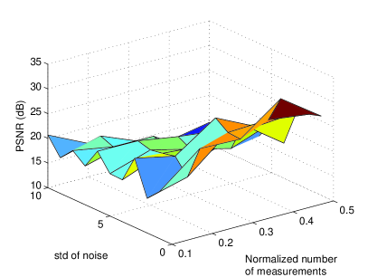
(a) GTCS-P

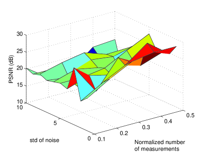
(b) KCS

Figure 7: PSNR for the tested methods in the scenario of recovering the sparse video in the presence of noise.

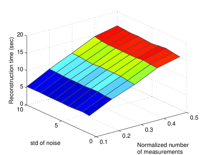
(a) GTCS-P

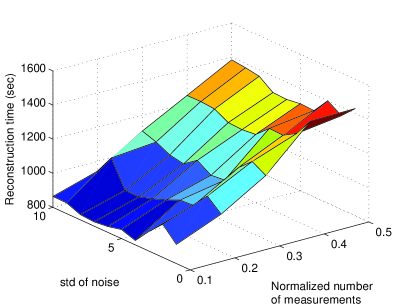
(b) KCS

Figure 8: Execution time for the tested methods in the scenario of recovering the sparse video in the presence of noise.

3.4 Tensor Compressibility

Let $\mathcal{X}=[x_{i_{1},\ldots,i_{d}}]\in\mathbb{R}^{N_{1}\times\ldots\times N_{d}}$. Assume the entries of the measurement matrix are drawn from a Gaussian or Bernoulli distribution as described above. For a given level of reconstruction accuracy, the number of measurements for $\mathcal{X}$ required by GTCS should satisfy

$$m\geq 2^{d}c^{d}\prod_{i\in[d]}\ln\frac{N_{i}}{k}.$$ (48)

Suppose that $N_{1}=\ldots N_{d}=N^{\frac{1}{d}}$. Then

$$m\geq 2^{d}c^{d}(\ln\frac{N^{\frac{1}{d}}}{k})^{d}=2^{d}c^{d}(\frac{1}{d}\ln N-\ln k)^{d}.$$ (49)

On the other hand, the number of measurements required by KCS should satisfy

$$m\geq 2c\ln\frac{N}{k}.$$ (50)

Note that the lower bound in Eq. (50) is indicative of a better compression ratio relative to that in Eq. (49). In fact, this phenomenon has been observed in simulations (see Ref. FLS13 ), which indicate that KCS reconstructs the data with better compression ratios than GTCS.

4 Conclusion

In applications involving color images, video sequences, and multi-sensor networks, the data is intrinsically of high-order, and thus more suitably represented in tensorial form. Standard applications of CS to higher-order data typically involve representation of the data as long vectors that are in turn measured using large sampling matrices, thus imposing a huge computational and memory burden. As a result, extensions of CS theory to multidimensional signals have become an emerging topic. Existing methods include Kronecker compressed sensing (KCS) for sparse tensors and multi-way compressed sensing (MWCS) for sparse and low-rank tensors. KCS utilizes Kronecker product matrices as the sparsifying bases and to represent the measurement protocols used in distributed settings. However, due to the requirement to vectorize multidimensional signals, the recovery procedure is rather time consuming and not applicable in practice. Although MWCS achieves more efficient reconstruction by fitting a low-rank model in the compressed domain, followed by per-mode decompression, its performance relies highly on the quality of the tensor rank estimation results, the estimation being an NP-hard problem. We introduced the Generalized Tensor Compressed Sensing (GTCS)–a unified framework for compressed sensing of higher-order tensors which preserves the intrinsic structure of tensorial data with reduced computational complexity at reconstruction. We demonstrated that GTCS offers an efficient means for representation of multidimensional data by providing simultaneous acquisition and compression from all tensor modes. We introduced two reconstruction procedures, a serial method (GTCS-S) and a parallelizable method (GTCS-P), both capable of recovering a tensor based on noiseless and noisy observations, and compared the performance of the proposed methods with Kronecker compressed sensing (KCS) and multi-way compressed sensing (MWCS). As shown, GTCS outperforms KCS and MWCS in terms of both reconstruction accuracy (within a range of compression ratios) and processing speed. The major disadvantage of our methods (and of MWCS as well), is that the achieved compression ratios may be worse than those offered by KCS. GTCS is advantageous relative to vectorization-based compressed sensing methods such as KCS because the corresponding recovery problems are in terms of a multiple small measurement matrices $U_{i}$’s, instead of a single, large measurement matrix $A$, which results in greatly reduced complexity. In addition, GTCS-P does not rely on tensor rank estimation, which considerably reduces the computational complexity while improving the reconstruction accuracy in comparison with other tensorial decomposition-based method such as MWCS.

Appendix

Let $X=[x_{ij}]\in\mathbb{R}^{N_{1}\times N_{2}}$ be $k$-sparse. Let $U_{i}\in\mathbb{R}^{m_{i}\times N_{i}}$, and assume that $U_{i}$ satisfies the NSP_k property for $i\in[2]$. Define $Y$ as

$$Y=[y_{pq}]=U_{1}XU_{2}^{T}\in\mathbb{R}^{m_{1}\times m_{2}}.$$ (51)

Given a rank decomposition of $X$, $X=\sum_{i=1}^{r}z_{i}u_{i}^{T}$, where $\mathrm{rank\;}(X)=r$, $Y$ can be expressed as

$$Y=\sum_{i=1}^{r}(U_{1}z_{i})(U_{2}u_{i})^{T},$$ (52)

which is also a rank-$r$ decomposition of $Y$, where $U_{1}z_{1},\ldots,U_{1}z_{r}$ and $U_{2}u_{1},\ldots,U_{2}u_{r}$ are two sets of linearly independent vectors.

Proof

Since $X$ is $k$-sparse, $\mathrm{rank\;}(Y)\leq\mathrm{rank\;}(X)\leq k$. Furthermore, both $R(X)$, the column space of $X$, and $R(X^{T})$ are vector subspaces whose elements are $k$-sparse. Note that $z_{i}\in R(X),u_{i}\in R(X^{T})$. Since $U_{1}$ and $U_{2}$ satisfy the NSP_k property, then $\dim(U_{1}R(X))=\dim(U_{2}R(X^{T}))=\mathrm{rank\;}(X)$. Hence the decomposition of $Y$ in Eq. (52) is a rank-$r$ decomposition of $Y$, which implies that $U_{1}z_{1},\ldots,U_{1}z_{r}$ and $U_{2}u_{1},\ldots,U_{2}u_{r}$ are two sets of linearly independent vectors. This completes the proof. ∎

References

- (1) Candes, E. J., Romberg, J. K., Tao, T.: Robust Uncertainty Principles: Exact Signal Reconstruction from Highly Incomplete Frequency Information. Information Theory, IEEE Transactions on , vol.52, no.2, pp.489-509, Feb. 2006
- (2) Donoho, D. L.: Compressed Sensing. Information Theory, IEEE Transactions on, vol.52, no.4, pp.1289-1306, Apr. 2006
- (3) Cohen, A., Dahmen, W., Devore, R.: Compressed Sensing and Best k-Term Approximation. J. Amer. Math. Soc., vol. 22, no.1, pp.211-231, 2009
- (4) Candes, E. J.: The Restricted Isometry Property and its Implications for Compressed Sensing. Comptes Rendus Math., vol.346, nos.9-10, pp.589-592, 2008
- (5) De Lathauwer, L., De Moor, B., Vandewalle, J.: A Multilinear Singular Value Decomposition, SIAM J. Matrix Anal. Appl., vol.21, pp.1253-1278, 2000
- (6) Duarte, M.F., Baraniuk, R.G.: Kronecker Compressive Sensing. Image Processing, IEEE Transactions on , vol.21, no.2, pp.494-504, Feb. 2012
- (7) Friedland, S., Li, Q., Schonfeld, D.: Compressive Sensing of Sparse Tensor, arXiv:1305.5777
- (8) Sidiropoulos, N.D., Kyrillidis, A.: Multi-Way Compressed Sensing for Sparse Low-Rank Tensors, Signal Processing Letters, IEEE ,vol.19, no.11, pp.757-760, Nov. 201
- (9) Golub, G. H., Charles, F. V. L.: Matrix Computations, fourth edition
- (10) Candes, E. J., Romberg, J. K.: The magic toolbox, available online: http://www.l1-magic.org
- (11) Candes,E. J., Romberg, J. K., Tao, T.: Stable Signal Recovery from Incomplete and Inaccurate Measurements, Communications on Pure and Applied Mathematics, Vol. LIX, pp. 1207-1223, 2006
- (12) Tucker, L. R: The Extension of Factor Analysis to Three-Dimensional Matrices, Contributions to mathematical psychology, 1964
- (13) Kolda, T. G., Bader, B. W.: Tensor Decompositions and Applications, SIAM REVIEW, vol. 51, no.3, pp. 455-500, 2009
- (14) Rauhut, Holger: Compressive Sensing and Structured Random Matrices, Radon Series Comp. Appl. Math XX, 1 C94
- (15) Donoho, D. L., Tsaig, Y.: Extensions of Compressed Sensing, Signal Processing, vol. 86, no.3, pp.533-548, Mar. 2006
- (16) Donoho, D.L., Tsaig, Y.: Fast Solution of -Norm Minimization Problems When the Solution May Be Sparse, Information Theory, IEEE Transactions on, vol.54, no.11, pp.4789-4812, Nov. 2008