A Ballistic Monte Carlo Approximation of $\pi$

Abstract

We compute a Monte Carlo approximation of $\pi$ using importance sampling with shots coming out of a Mossberg 500 pump-action shotgun as the proposal distribution. An approximated value of $3.131$ is obtained, corresponding to a $0.33\%$ error on the exact value of $\pi$. To our knowledge, this represents the first attempt at estimating $\pi$ using such method, thus opening up new perspectives towards computing mathematical constants using everyday tools.

I Introduction

The ratio between a circle’s circumference and its diameter, named $\pi$, is a mathematical constant of crucial importance to science, yet most scientists rely on pre-computed approximations of $\pi$ for their research. This is problematic, because scientific progress relies on information that will very likely disappear in case of a cataclysmic event, such as a zombie apocalypse. In such case, scientific progress might even stop entirely. This motivates the need for a robust, yet easily applicable method to estimate $\pi$.

We first lay down the theoretical framework for Monte Carlo methods, including importance sampling and propose a probabilistic interpretation of $\pi$ within this framework. We then introduce the idea of computing $\pi$ using importance sampling with a ballistic-based proposal distribution and suggest a robust way of dealing with the unknown generating distribution. Finally, we compare the obtained estimation of $\pi$ with the true value.

I.1 Monte Carlo

The Monte Carlo method, first introduced in Metropolis and Ulam (1949), is a stochastic approach to computing expectations of functions of random variables. Let $f(\mathbf{x}):\mathbb{R}^{n}\rightarrow\mathbb{R}^{+}$ be a probability density function over a random vector $\mathbf{x}\in\mathbb{R}^{n}$ and let $g(\mathbf{x}):\mathbb{R}^{n}\rightarrow\mathbb{R}$ be a function of $\mathbf{x}$.

The expected value $\mathbb{E}$ of $g$ over $f$ is defined as

$$\mathbb{E}_{f}[g(\mathbf{x})]=\int_{\mathbb{R}^{n}}f(\mathbf{x})g(\mathbf{x})d\mathbf{x}.$$ (1)

The Monte Carlo method approaches $\mathbb{E}_{f}[g(\mathbf{x})]$ with

$$\mathbb{E}_{f}[g(\mathbf{x})]\approx\hat{\mathbb{E}}_{f}[g(\mathbf{x})]=\frac{1}{N}\sum_{i=1}^{N}g(\mathbf{x}_{i}),\quad\mathbf{x}_{i}\sim f(\mathbf{x})$$ (2)

where $\mathbf{x}_{i}\sim f(\mathbf{x})$ means $\mathbf{x}_{i}$ is drawn $f(\mathbf{x})$.

Note that $\hat{\mathbb{E}}_{f}[g(\mathbf{x})]$ is a consistent estimator of $\mathbb{E}_{f}[g(\mathbf{x})]$, i.e. $\hat{\mathbb{E}}_{f}[g(\mathbf{x})]$ converges in probability to $\mathbb{E}_{f}[g(\mathbf{x})]$ as $N\rightarrow\infty$. Furthermore, its variance decreases as $\frac{1}{N}$ independently of the dimensionality of $\mathbf{x}$. For more details, see Bishop (2006).

I.2 Importance sampling

When sampling from $f(\mathbf{x})$ is difficult or impossible, or when $f(\mathbf{x})$ is too different from $g(\mathbf{x})$ (i.e. high probability mass regions correspond to a low-valued $g(\mathbf{x})$ and vice-versa), Monte Carlo methods may fail. In that case, we note that

$$\begin{split}\mathbb{E}_{f}[g(\mathbf{x})]&=\int_{\mathbb{R}^{n}}f(\mathbf{x})g(\mathbf{x})d\mathbf{x}\\ &=\int_{\mathbb{R}^{n}}q(\mathbf{x})\frac{f(\mathbf{x})}{q(\mathbf{x})}g(\mathbf{x})d\mathbf{x}\\ &=\mathbb{E}_{q}\left[\frac{f(\mathbf{x})}{q(\mathbf{x})}g(\mathbf{x})\right]\\ \end{split}$$ (3)

for some arbitrary distribution $q(\mathbf{x})$ such that $q(\mathbf{x})>0$ when $f(\mathbf{x})g(\mathbf{x})\neq 0$. We can therefore reformulate the approximation as

$$\begin{split}\mathbb{E}_{f}[g(\mathbf{x})]&\approx\hat{\mathbb{E}}_{q}\left[\frac{f(\mathbf{x})}{q(\mathbf{x})}g(\mathbf{x})\right]\\ &=\frac{1}{N}\sum_{i=1}^{N}\frac{f(\mathbf{x}_{i})}{q(\mathbf{x}_{i})}g(\mathbf{x}_{i}),\quad\mathbf{x}_{i}\sim q(\mathbf{x}).\end{split}$$ (4)

This method is called importance sampling, and given a careful choice of $q(\mathbf{x})$, can allow easier sampling and help reduce the variance of the estimator. We note once again that $\hat{\mathbb{E}}_{q}\left[\frac{f(\mathbf{x})}{q(\mathbf{x})}g(\mathbf{x})\right]$ is a coherent estimator of $\mathbb{E}_{f}[g(\mathbf{x})]$. For more details, see Bishop (2006).

I.3 Introducting $\pi$ in the Monte Carlo framework

Figure 1: $\pi$ is proportional to the area of a unit square occupied by a quarter circle of radius $1$.

By choosing an appropriate probability density function $f(\mathbf{x})$ and an appropriate function $g(\mathbf{x})$, the value of $\pi$ can be approached using a Monte Carlo estimation.

Consider a unit square and a circle arc joining two opposite corners of the square (Fig. 1). The area of the square is $1$, while the area of the quarter circle is $\frac{\pi}{4}$, which means the proportion of the square’s area occupied by the quarter circle is also $\frac{\pi}{4}$. In other words,

$$\int_{0}^{1}\int_{0}^{1}g(x,y)dxdy=\frac{\pi}{4}$$ (5)

with

$$g(x,y)=\begin{cases}1,\quad x^{2}+y^{2}\leq 1,\\ 0,\quad\text{otherwise}.\end{cases}$$ (6)

We rewrite equation 5 as

$$\int_{-\infty}^{\infty}\int_{-\infty}^{\infty}f(x,y)g(x,y)dxdy=\frac{\pi}{4}$$ (7)

with

$$f(x,y)=\begin{cases}1,\quad 0\leq x\leq 1\text{ and }0\leq y\leq 1,\\ 0,\quad\text{otherwise}\end{cases}$$ (8)

and observe that it is identical in form to equation 1. Therefore the numerical value of $\pi$ can be interpreted as the expected value of $g(\mathbf{x})$ with $\mathbf{x}$ being a random two-dimensional vector uniformly distributed over the unit square.

This allows us to approximate equation 7 as

$$\begin{split}\frac{\pi}{4}\approx\hat{\mathbb{E}}_{f}[g(\mathbf{x})]&=\frac{1}{N}\sum_{i=1}^{N}g(\mathbf{x}_{i}),\\ \mathbf{x}_{i}\sim f(\mathbf{x})&=\mathcal{U}([0,1]\times[0,1])\end{split}$$ (9)

In other words, to approximate $\frac{\pi}{4}$, one needs to draw $N$ uniformly-distributed samples across the unit square and count the proportion of those points which fall into the quarter circle.

I.4 Off-the-shelf random sampling

Figure 2: Experimental setup. The shotgun is pointed at an aluminum foil to record its shot pattern. Samples are iteratively drawn by shooting the shotgun.

In order to estimate $\pi$ using a Monte Carlo method, one needs to draw independent and identically-distributed (IID) samples from a uniform distribution. While computer-assisted pseudo-random number generation is computationally cheap and fast, it relies on technology which might not be available in the event of a zombie apocalypse.

On the other hand, primitive methods such as coin tosses or dice throws are almost always readily available, but they are slow and their sampling time scales linearly with the numerical precision required.

With this in mind, we advocate the use of ballistic-assisted (i.e. projectile-based) random sampling methods because they are both easily accessible and parallelizable. In particular, shotgun-assisted random sampling seems very suitable because of the presumed abundance of shotguns in cataclysmic times and the speed at which they can generate samples.

To our knowledge, no prior attempt at estimating $\pi$ using ballistic-assisted random sampling methods has ever been made.

I.5 Uniformity issue

There is no guarantee that shotgun shots are uniformly distributed. In fact, pellet distribution depends on many latent variables such as height of the shooter, distance to the target, orientation of the shotgun and wind direction, to name a few. The issue can be overcome by using importance sampling, but the shot distribution is unknown, and will need to be estimated in order for importance sampling to work.

Since this instance of density estimation problem is low-dimensional, a simple histogram method is sufficient. The bin width hyperparameter can be decided using cross-validation on the log-likelihood of the samples.

Thus $\frac{\pi}{4}$ can be computed as

$$\begin{split}\frac{\pi}{4}\approx\hat{\mathbb{E}}_{f}\left[\frac{f(\mathbf{x})}{\hat{q}(\mathbf{x})}g(\mathbf{x})\right]&=\frac{1}{N}\sum_{i=1}^{N}\frac{g(\mathbf{x}_{i})}{\hat{q}(\mathbf{x}_{i})},\\ \mathbf{x}_{i}\sim q(\mathbf{x})\end{split}$$ (10)

where $\hat{q}(\mathbf{x})$ is the histogram estimate of the probability density function (PDF).

II Experimental setup

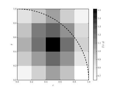
Figure 3: An estimate of the probability density function of the data points obtained using a 2D histogram method with a bin width of $0.2$ on $10000$ randomly-selected samples. A quarter circle was drawn for visual reference.

To sample from the proposal distribution, a 28-inch-barrel Mossberg 500 shotgun was used. The latter is chambered for 3 inches, 12-gauge shotshells and its spread can be tuned by using different types of chokes mounted at the end of the barrel.

For this experiment, we used an improved cylinder choke made by Mossberg. Cartriges used were composed of 3 dram equivalent of powder and 32 grams of #8 lead pellets. Average muzzle velocity is estimated to be around $366m/s$ by the manufacturer.

Samples were recorded by placing an aluminum foil in the trajectory of the shots (Fig. 2). The shotgun was fired at a $20m$ distance from the targets.

Foils were photographed and samples were extracted by locating holes in the image and computing their center of mass. Sample positions were normalized to be in $[0,1]\times[0,1]$ .

III Results

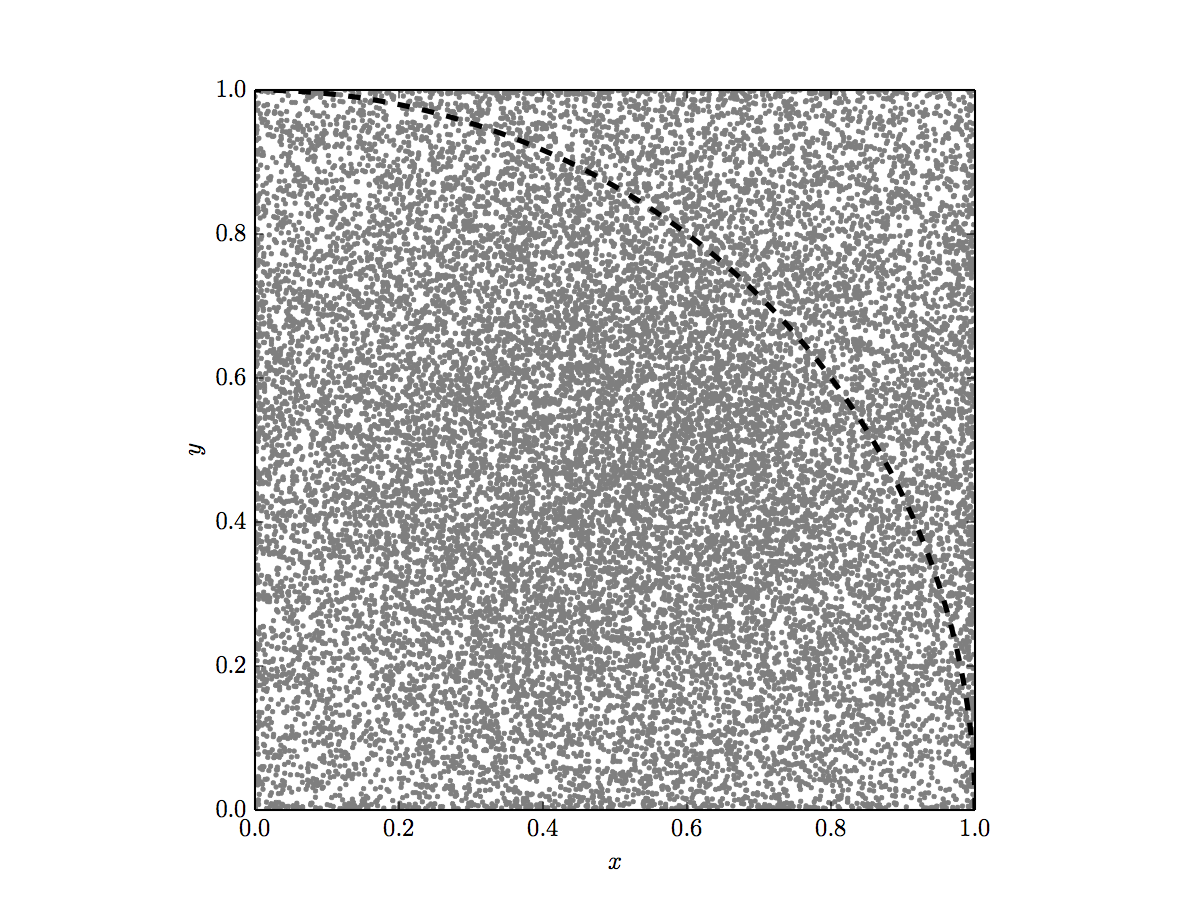
Figure 4: Remaining $20857$ samples used to approximate $\pi$. Positions were normalized to be in $[0,1]\times[0,1]$. A quarter circle was drawn for visual reference.

The experiment described above was carried by firing 200 shots, yielding $30857$ samples.

The sample extraction method described in section II could not distinguish holes made by one or many pellets. One sample might actually correspond to many pellet impacts, or even a wad impact, but this factor of variation is integrated in the PDF estimation.

Of the $30857$ samples produced, we used a random subset of $10000$ samples for PDF estimation. The optimal bin width hyperparameter was determined to be $0.2$ using 20-fold cross-validation. The estimated PDF of the shot distribution is shown in Fig. 3.

Using equation 10 on the $20857$ remaining samples (Fig. 4), a value of $3.131$ for $\pi$ was obtained, which corresponds to a $0.33\%$ error on the true value.

IV Conclusion

We successfully estimated the value of $\pi$ using a Monte Carlo method by drawing samples from shots coming out of a Mossberg 500 pump-action shotgun. Non-uniformity of pellet spread was accounted for by importance sampling. The pellet distribution was approximated using a 2D histograms method.

While variance on the estimate could be reduced by drawing more samples, this is still a striking display of the robustness of Monte Carlo methods: even though pellet distribution depended on many uncontrolled factors (wind direction, muzzle orientation, aluminium foil geometry, and wad impacts to name a few), the approached value of $\pi$ ($3.131$) is still within $0.33\%$ of the true value.

We feel confident that ballistic Monte Carlo methods such as the one presented in this paper constitute reliable ways of computing mathematical constants should a tremendous civilization collapse occur.