Observation of spectral interference for any path difference in an interferometer

Abstract

We report the experimental observation of spectral interference in a Michelson interferometer, regardless of the relationship between the temporal path difference introduced between the arms of the interferometer and the spectral width of the input pulse. This observation is possible by introducing the polarization degree of freedom into a Michelson interferometer using a typical weak value amplification scenario.

¹ICFO-Institut de Ciencies Fotoniques, Mediterranean Technology Park, 08860 Castelldefels (Barcelona), Spain
² Quantum Optics Laboratory, Universidad de los Andes, AA 4976, Bogotá, Colombia
³ Department of Signal Theory and Communications, Universitat Politecnica de Catalunya, 08034 Barcelona, Spain

^∗Corresponding author: luis-jose.salazar@icfo.es

260.0260, 260.3160,260.5430, 320.5550,120.3180

Interference is a fundamental concept in any theory based on waves, such as classical electromagnetism or quantum theory. The specific experimental arrangement required for the observation of interference depends on the characteristics of the light source, i.e., its spatio-temporal profile and its degree of coherence. For example, for first-order coherent light in a Michelson interferometer, for temporal delays shorter than the pulse width, interference manifests as a delay-dependent change of the intensity at the output port of the interferometer. For longer temporal delays, interference manifest as spectral interference for a given temporal delay. The observation of spectral interference was denoted by Mandel  [1, 2] as the Alford-Gold effect [3] and it is well- known in optics [4].

Here we report the observation of spectral interference independently of the temporal regime under consideration. The interference is revealed as a reshaping of the input spectrum that is accomplished by introducing the polarization degree of freedom into a Michelson interferometer. This scenario corresponds precisely to the conditions of a typical weak value amplification configuration [5, 6, 7, 8] that although was originally conceived in the framework of a quantum formalism, it is essentially based on the phenomena of interference and can thus be applied to any scenario with waves [9, 10, 11, 12, 13].

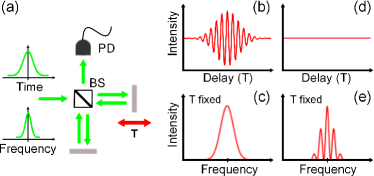
Figure 1: Typical interference patterns that can be observed in a Michelson interferometer, in the time and frequency domains. (a) depicts the interferometric configuration considered. BS: beam splitter, PD: Photodetector. (b) and (d) show the intensity measured as a function of a temporal delay $T$. (c) and (e) show the intensity as a function of frequency for a given value of $T$. (b) and (c) correspond to the case $T\ll\tau$, while (d) and (e) correspond to the case, $T\gg\tau$.

For the sake of clarity, let us start by describing temporal and spectral interference in a typical Michelson interferometer, without considering polarization. Later on, we will describe the effects that the introduction of the polarization degree of freedom has on spectral interference. Consider the situation depicted in Fig. 1(a). A first-order coherent input pulse with amplitude $E_{0}$, central frequency $\nu_{0}$, input polarization ${\bf e}_{in}$, and temporal duration $\tau$ (full width at half maximum) described by

$${\bf E}_{in}(t)=E_{0}\,\exp\left[-(2\ln 2/\tau^{2})\,t^{2}+i\,2\pi\nu_{0}t\right]\,{\bf e}_{in}\,,$$ (1)

enters a Michelson interferometer where is divided in two beams by a beam splitter (BS). Each of the new pulses follows a different path and after reflection in a mirror the two pulses recombine at the BS. By changing the position of one of the mirrors, a temporal delay ($T$) is generated between the two pulses. The intensity measured by a slow detector at the output port of the interferometer as a function of $T$ can be written as

$$I(T)=\frac{I_{0}}{2}\,\left[1+\exp\left(-\ln 2\,T^{2}/\tau^{2}\right)\,\cos\left(2\pi\nu_{0}T\right)\right]\,,$$ (2)

where $I_{0}=|E_{0}|^{2}$. Two interesting cases can be distinguished: i) when $T\ll\tau$, and therefore, the two pulses traveling the different paths overlap in time and ii) when $T\gg\tau$ and the two pulses do not overlap. In the first case, the output intensity as a function of $T$ reduces to

$$I_{T\ll\tau}(T)=\frac{I_{0}}{2}\,[1+\cos(2\pi\nu_{0}T)],$$ (3)

while in the case $T\gg\tau$, Eq. (2) becomes

$$I_{T\gg\tau}(T)=\frac{I_{0}}{2}\,.$$ (4)

These results are very well known in optics. They indicate the presence of temporal interference for the case $T\ll\tau$ and its absence for $T\gg\tau$. The two situations are illustrated in Fig. 1(b) and Fig. 1(d).

An analogous analysis can be done when the detector in Fig. 1(a) is changed by a spectrometer and the power spectrum $S(\nu)$ as a function of the frequency $\nu$ is considered. In this case,

$$S(\nu)=\frac{S_{in}(\nu)}{2}\left[1+\cos\left(2\pi\nu\,T\right)\right]\,,$$ (5)

where

$$S_{in}(\nu)=S_{0}\exp\left[-(\pi^{2}\tau^{2}/\ln 2)(\nu-\nu_{0})^{2}\right]\,$$ (6)

is the input power spectrum with $S_{0}$ being a constant.

Equation (5) indicates that $S(\nu)$ corresponds to a reshaping of the input spectrum. This reshaping can be understood if $h(\nu)=\tfrac{1}{2}[1+\cos(2\pi\nu\,T)]$ is considered as a transfer function that describes the effect of the interferometer. Therefore depending on the relationship between the oscillation frequency of the transfer function, defined by $T$, and the pulse width, $\tau$, it is possible to obtain different reshapings of the input spectrum that can be identified with interference. Fig. 1(c) and Fig. 1(e) depict the output power spectrum for the regime $T\ll\tau$ and $T\gg\tau$, respectively. The two cases are clearly different. As expected from standard interferometry, when $T\ll\tau$, the output power spectrum, is identical to the input one, while for $T\gg\tau$, a clear reshaping of the input spectrum appears. This last case corresponds to the Alford-Gold effect and indicates that a Michelson interferometer can be seen as a periodic filter that produces a modulation of the initial spectrum with a peak separation proportional to $\sim 1/T$.

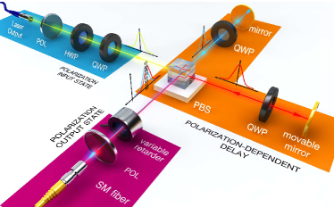
Figure 2: Experimental setup. The input pulse polarization state is selected to be left-circular by using a polarizer, a quarter wave plate (QWP) and a half wave plate (HWP). A Polarizing beam splitter (PBS) splits the input into two orthogonal linear polarizations that propagate along different arms of the interferometer. An additional QWP is introduced in each arm to rotate the beam polarization by $90^{\circ}$ to allow the recombination of both beams in a single beam by the same PBS. The output beam spectrum is measured by an optical spectrum analyzer (OSA) connected to a single mode fiber (SM).

Now let us describe the effects of adding the polarization degree of freedom to the Michelson interferometer. For this, consider the situation depicted in Fig. 2 in which four main differences with the standard Michelson interferometer of Fig. 1(a) can be observed: $1)$ the presence of polarization control elements in the input port of the interferometer, $2)$ the substitution of the beam splitter (BS) by a polarizing beam splitter (PBS), $3)$ the introduction of a quarter wave plate (QWP) in each arm of the interferometer, and $4)$ the presence, in the output port, of a variable polarization analyzer, composed by a liquid crystal variable retarder (LCVR) and a polarizer at $45^{\circ}$. The polarizer, half-wave plate and quarter wave plate in the interferometer’s input port are used to set up the polarization of the input beam. The PBS divides spatially the two orthogonal polarization components of the input beam and the QWP rotates the corresponding polarization component by $90^{\circ}$ after reflection in each mirror. The movable mirror generates the temporal delay $T$.

Since two beams with orthogonal polarizations do not interfere, an interference effect is generated by the polarization control elements of the output port that generate an additional phase difference, $\Gamma$, between the pulses coming from the two paths of the interferometer. In particular, for a left-handed circularly polarized input beam $({\bf e}_{in}={\bf x}-i{\bf y})$, where ${\bf x}$ denotes horizontal polarization and ${\bf y}$ vertical polarization, the output electric field reads

$${\bf E}_{out}(\nu)=E_{0}\sqrt{\frac{\pi\tau^{2}}{4\ln 2}}\exp\left\{-[\pi^{2}\tau^{2}/(2\ln 2)]\,(\nu-\nu_{0})^{2}\right\}$$

$$\times\left\{\exp\left(-i\,2\pi\nu T\right){\bf x}+\exp\left[-i\,\left(\Gamma+\pi/2\right)\right]{\bf y}\,\right\}.$$ (7)

The power spectrum of the light at the interferometer’s output port is then given by

$$S_{out}(\nu)=\frac{S_{in}(\nu)}{2}\left[1+\cos\left(2\pi\nu\,T-\Gamma-\pi/2\right)\right]\,.$$ (8)

In the same way as was done for Eq. (5), it is possible to identify from Eq. (8) a transfer function, $H(\nu)=\tfrac{1}{2}[1+\cos(2\pi\nu\,T-\Gamma-\pi/2)]$, and distinguish two cases depending on the relationship between the frequency of oscillation of $H(\nu)$ and the width of the input power spectrum. We illustrate in the first column of Figs. 3 and 4 various transfer functions (dashed lines) for different values of $\Gamma$ and $T$ and the measured power spectrum of a pulsed laser (solid line) with a temporal duration $\tau=320\,\mathrm{fs}$ and central frequency $\nu_{0}=193.5\,\mathrm{THz}$. We observe that while for the case $T\gg\tau$ (Fig. 3) various oscillations of the transfer function fit inside the initial spectrum bandwidth, for $T\ll\tau$ (Fig. 4) this is not the case. This fact results in an output spectrum that corresponds to different kinds of reshapings of the input spectrum depending on the regime $T\gg\tau$ or $T\ll\tau$. However, it is important to notice that for all regimes the reshaping of the spectrum is the result of an interference effect and therefore indicates that spectral interference can be observed in a Michelson interferometer, independently of the temporal path difference under consideration, when the polarization degree of freedom is considered in the interferometer.

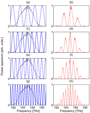
Figure 3: Spectral interference in the regime $T\gg\tau$. First column depicts theoretical transfer function, $H(\nu)$, as a dashed line for $\Gamma=61.5^{\circ}$ and different time delays: $T=1453\,\mathrm{fs}$ in (a), $T=2120\,\mathrm{fs}$ in (c), $T=2786\,\mathrm{fs}$ in (e) and $T=4120\,\mathrm{fs}$ in (g). The solid line corresponds to the measured spectrum of a pulsed laser with a temporal duration $\tau=320\,\mathrm{fs}$ centered in $\nu_{0}=193.5\,\mathrm{THz}$. Second column shows the experimental results for $S_{\mathrm{out}}(\nu)$. The vertical dashed line indicates the central frequency of the input spectrum.

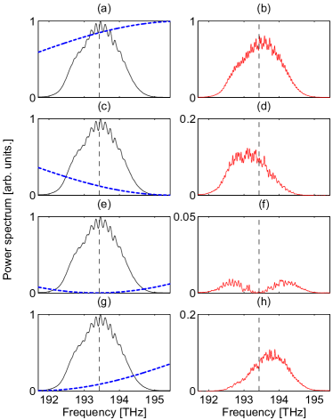
Figure 4: Spectral interference in the regime $T\ll\tau$. First column depicts theoretical transfer function, $H(\nu)$, as a dashed line for a fixed delay of $T=53.7\,\mathrm{fs}$ and $\Gamma=98.5^{\circ}$ in (a), $\Gamma=273.1^{\circ}$ in (c), $\Gamma=231.2^{\circ}$ in (e), and $\Gamma=198.9^{\circ}$ in (g). The solid line corresponds to the measured spectrum of a pulsed laser with a temporal duration $\tau=320\,\mathrm{fs}$ centered in $\nu_{0}=193.5\,\mathrm{THz}$. Second column shows the experimental results for $S_{\mathrm{out}}(\nu)$. The vertical dashed line indicates the central frequency of the input spectrum. To help the eye the vertical axis has been reescaled since the output intensity changes dramatically with different values of $\Gamma$ in this regime.

To check experimentally that spectral interference can be observed independently of the value of $T$, the setup of Fig. 2, based only on linear optical elements, was implemented. An input pulse (Calmar Laser - Mendocino) with a temporal duration $\tau=320\,\mathrm{fs}$, repetition rate of $20\,\mathrm{MHz}$ and central frequency $\nu_{0}=193.5\,\mathrm{THz}$ ($1550\,\mathrm{nm}$) is prepared with left-handed circular polarization, ${\bf e}_{in}={\bf x}-i\,{\bf y}$, by using the combination of a polarizer, HWP and QWP. The PBS splits the input beam into two beams with orthogonal polarizations and, as mentioned before, each polarization component is rotated by $90^{\circ}$ by using the QWP and the corresponding a mirror. The movable mirror, mounted on a translation stage, allows to change the temporal delay $T$ between pulses with orthogonal polarizations. The PBS recombines the two reflected beams in a single beam that emerges from the PBS, passes through the LCVR followed by a polarizer, and is finally focused into a single mode fiber (SM) and its spectrum is measured with an Optical Spectrum Analyzer (Yokogawa - AQ6370).

The second column of Figs. 3 and 4 shows the experimental results for $T\gg\tau$ and $T\ll\tau$, respectively. A reshaping of the spectrum is clearly observed in both cases. For the case of $T\gg\tau$, a clear modulation with a spacing between peaks proportional to $1/T$ is observed corresponding to the Alford-Gold effect. For the regime $T\ll\tau$, two situations can be distinguished, both accompanied by different amount of losses. In some cases the reshaping corresponds to a modulation of the initial spectrum [Fig. 4(f)], while in other the reshaping of the spectrum translate into a measurable shift of the central frequency of the output power spectrum when compared with the central frequency of the input pulse [Fig. 4(d) and (h)] [10, 12, 13].

In conclusion, we have shown that spectral interference can also be observed in the regime of small optical path differences ($T\ll\tau$). This result complements the observation of the Alford-Gold effect, which reveals interference in the frequency domain in the opposite regime, $T\gg\tau$. The observation of spectral interference, regardless the temporal path difference, was made possible by introducing the polarization variable in a Michelson interferometer in an experimental scheme similar to the ones used in a weak measurement scenario. The presence of interference in the regime $T\gg\tau$ appears as a clear modulation of the frequency spectrum with frequency $\sim 1/T$ [see Figs. 3(b), (d), (f) and (h)], while in the case $T\ll\tau$, interference manifests as a modulation of the input spectrum [Fig. 4(f)] or as a shift of the central frequency [Figs. 4(b), (d) and (h)].

Acknowledgements: We acknowledge support from the Spanish government projects FIS2010-14831 and Severo Ochoa programs, and from Fundació Privada Cellex, Barcelona. LJSS and AV acknowledges support from Facultad de Ciencias, Universidad de los Andes Bogotá, Colombia.

References

- [1] M. P. Givens, “Photoelectric Detection of Interference between Two Light Beams Having a Large Path Difference,” J. Opt. Soc. Am. 51, 1030–1032 (1961).
- [2] L. Mandel, “Interference and the Alford and Gold Effect,” J. Opt. Soc. Am. 52, 1335–1339 (1962).
- [3] W. P. Alford and A. Gold, “Laboratory Measurement of the Velocity of Light,” Am. J. Phys. 26, 481–484 (1958).
- [4] X. Y. Zou, T. P. Grayson ansd L. Mandel, “Observation of quantum interference effects in the frequency domain,” Phys. Rev. Lett. 69, 3041–3044 (1992).
- [5] Y. Aharonov, D. Z. Albert, and L. Vaidman, “How the result of a measurement of a component of the spin of a particle can turn out to be 100,” Phys. Rev. Lett. 60, 1351–1354 (1988).
- [6] I. M. Duck, P. M. Stevenson, and E. C. G. Sudarhshan, “The sense in which a “weak measurement” of a spin particle’s spin component yields a value of 100,” Phys. Rev. D 40, 2112–2117 (1989).
- [7] J. Dressel, M. Malik, F. M. Miatto, A. N. Jordan, and R. W. Boyd, “Colloquium: Understanding quantum weak values: Basics and applications,” Rev. Mod. Phys. 86, 307–316 (2014).
- [8] A. N. Jordan, J. Martinez-Rincon, and J. C. Howell, “Technical Advantages for Weak-Value Amplification: When Less Is More,” Phys. Rev. X 4, 011031, (2014).
- [9] J. C. Howell, D. J. Starling, P. Ben Dixon, P. K. Vudyasetu, and A. N. Jordan, “Interferometric weak value deflections: Quantum and classical treatments,” Phys. Rev. A 81, 033813 (2010).
- [10] N. Brunner and C. Simon, “Measuring small longitudinal phase shifts: weak measurements of standard interferometry,” Phys. Rev. Lett. 105 010405 (2010).
- [11] C.-F. Li, X.-Y. Xu, J.-S. Tang, J.-S. Xu, G.-C. Guo, “Ultrasensitive phase estimation with white light,” Phys. Rev. A 83, 044102 (2011).
- [12] X.-Y. Xu, Y. Kedem, K. Sun, L. Vaidman, C.-F. Li and G.-C. Guo, “Phase Estimation with Weak Measurement Using a White Light Source,” Phys. Rev. Lett. 111, 033604 (2013).
- [13] L. J. Salazar-Serrano, D. Janner, N. Brunner, V. Pruneri, J. P. Torres, “Measurement of sub-pulse-width temporal delays via spectral interference induced by weak value amplification ,” Phys. Rev. A 89 012126 (2014).