Trajectory and distribution of suspended non-Brownian particles moving past a fixed spherical or cylindrical obstacle

Abstract

We investigate the motion of a suspended non-Brownian sphere past a fixed cylindrical or spherical obstacle in the limit of zero Reynolds number for arbitrary particle-obstacle aspect ratios. We consider both a suspended sphere moving in a quiescent fluid under the action of a uniform force as well as a uniform ambient velocity field driving a freely suspended particle. We determine the distribution of particles around a single obstacle and solve for the individual particle trajectories to comment on the transport of dilute suspensions past an array of fixed obstacles. First, we obtain an expression for the probability density function governing the distribution of a dilute suspension of particles around an isolated obstacle, and we show that it is isotropic. We then present an analytical expression – derived using both Eulerian and Lagrangian approaches – for the minimum particle-obstacle separation attained during the motion, as a function of the incoming impact parameter, i.e. the initial offset between the line of motion far from the obstacle and the coordinate axis parallel to the driving field. Further, we derive the asymptotic behaviour for small initial offsets and show that the minimum separation decays exponentially. Finally we use this analytical expression to define an effective hydrodynamic surface roughness based on the net lateral displacement experienced by a suspended sphere moving past an obstacle.

1 Introduction

The interaction between suspended particles and obstacles encountered in their flow is essential for the understanding of the transport of particulate suspensions in natural porous systems as well as in engineered porous media used in different applications. In porous media, the behaviour of individual particles at the ‘pore-scale’ determines the migration, dispersion and ultimate fate of suspended particles (Lee & Koplik, 1999). Lagrangian methods in filtration theory, for example, rely on calculating the trajectory of individual particles in simplified representations of the pore space (Spielman, 1977; Adamczyk, 1989a; Ryan & Elimelech, 1996; Jegatheesan & Vigneswaran, 2005). Particle capture by single cylindrical and spherical collectors is investigated to understand filtration in fibrous media and packed beds, respectively (Spielman, 1977). In many filtration methods, such as deep bed filtration, the particles are typically smaller than the characteristic scale of the pores, and get collected or deposited onto the obstacles in their path. In order to gain insight into these systems, several studies have focused on the trajectories followed by small particles near large spherical or cylindrical collectors (Adamczyk & van de Ven, 1981; Adamczyk, 1989a, b; Goren & O’Neill, 1971; Gu & Li, 2002; Li & Marshall, 2007). Trajectory studies have also shown that not only particle capture but transit times may also be dominated by single particle-obstacle interactions (Lee & Koplik, 1999). Other studies modelling particle transport in porous media have focused on the similar problem of the trajectory followed by individual particles as they move through narrow channels, such as in the constricted-tube model (Burganos et al., 1992, 2001; Chang et al., 2003). Studies of particle migration, dispersion and capture using Eulerian methods also rely on calculating the detailed particle-fibre or particle-grain interactions in model porous media (Koch et al., 1989; Phillips et al., 1989, 1990; Shapiro et al., 1991; Nitsche, 1996). In this work, we investigate the properties of particle trajectories as the particles move past a fixed spherical or cylindrical obstacle driven by either a constant force or a uniform velocity field in the presence of particle-obstacle hydrodynamic interactions and for arbitrary particle-to-obstacle size ratios.

Recently, with the advent of microfluidic technology, there is a renewed interest in the understanding and characterization of the motion of individual particles past solid obstacles. The possibility of designing the stationary media with nearly arbitrary geometry and chemistry, with features of micron and sub-micron size, has led to microfluidic separation techniques that are primarily based on the species-specific particle-obstacle interactions. In deterministic lateral displacement, for example, a mixture of suspended particles driven through a two-dimensional (2D) periodic array of cylindrical obstacles spontaneously fractionates as different species migrate in different directions (Huang et al., 2004). The migration angle depends on the particle-obstacle interactions, and can be accurately described based on the trajectory followed by individual particles as they move past a fixed obstacle (Frechette & Drazer, 2009; Balvin et al., 2009; Herrmann et al., 2009; Bowman et al., 2012). Particle-obstacle interactions are also essential in separation methods based on ratchet effects induced by asymmetric arrays of obstacles (Li & Drazer, 2007). Other methods, such as pinched flow fractionation (Yamada et al., 2004) and some particle focusing systems (Hewitt & Marshall, 2010; Xuan et al., 2010) can also be investigated from the perspective of particle-obstacle interactions and the effect that both hydrodynamic and non-hydrodynamic forces have on the trajectories followed by different species (Luo et al., 2011). In all cases, the individual particle trajectories or the asymptotic distribution of suspended particles as they are driven past spherical or cylindrical obstacles contains the information necessary for calculation of the relevant average transport properties, such as migration speed and angle. However, an analytical treatment describing these two aspects of particle motion has not been developed. In this work, we provide such an analysis, within the purview of low Reynolds number hydrodynamics, wherein Stokes’ equations are assumed to describe the motion of the fluid, and particle inertia is neglected. Further, we consider the non-Brownian regime, since in many applications – separation devices in particular – high throughput is advantageous, leading to a routine occurrence of high Péclet numbers and the motion of the particles can be approximated as deterministic.

In addition, the results derived here are of relevance to suspension rheology and flows, specially in active micro-rheology, where a probe particle is driven through a quiescent suspension of particles. In turn, we shall show that it is possible to extend analytical results established in suspension rheology to the motion of a spherical particle driven past a fixed obstacle. In suspension flows, each individual particle is moving through a random distribution of other spheres. Furthermore, in the dilute approximation, the analysis of the relative motion (and distribution) between any two spheres of the suspension suffices to characterize its properties. Such a relative motion is analogous to the problem of a sphere moving with respect to a fixed obstacle in – say, for example – a microfluidic device. (Note that in the latter case the dilute approximation assumes not only a dilute suspension but also that the distance between obstacles is sufficiently large.) Therefore, before proceeding, it is convenient to briefly review some of the most relevant results concerning two-particle interactions in the limit of zero Reynolds and infinite Péclet numbers. Batchelor & Green (1972) first obtained the pair distribution function of spheres in a sheared suspension. Batchelor later extended his work by deriving the pair-distribution function in the case of a sedimenting polydispersed suspension of spheres (Batchelor, 1982; Batchelor & Wen, 1982; Batchelor, 1983). Davis & Hill (1992) used the resulting expression for the pair distribution function to analyze the hydrodynamic diffusion of a sphere sedimenting through a dilute suspension of neutrally buoyant particles. Almog & Brenner (1997) further employed the same pair distribution function to study the apparent viscosity experienced by a sphere moving through a quiescent suspension. They considered both the micro-rheological setting of a ‘falling ball viscometer’ as well as a non-rotating sphere moving with a prescribed velocity through the suspension. Khair & Brady (2006) studied the motion of a single Brownian particle through a suspension, and extended the analysis of Batchelor (1982) to obtain the pair-probability distribution function for finite Péclet numbers.

In this work, we consider the trajectory followed by a suspended particle driven by a constant external force (e.g. buoyancy force) or a uniform velocity field as it moves past a fixed sphere or cylinder in the limit of zero Reynolds and infinite Péclet numbers. We derive an expression for the minimum particle-obstacle separation attained during the motion, as a function of the incoming impact parameter between the sphere trajectory and the centre of the obstacle (offset $b_{in}$ in figure 1). The minimum distance between the particle and obstacle surfaces, that would result from a trajectory determined solely based on hydrodynamic interactions, dictates the relevance of short-range non-hydrodynamic interactions such as van der Waals forces, surface roughness (solid-solid contact), etc. In fact, the resulting scaling relation derived for small $b_{in}$ shows that extremely small surface-to-surface separations would be common during the motion of a particle past a distribution of periodic or random obstacles. This highlights the impact that short-range non-hydrodynamic interactions could have in the effective motion of suspended particles. In this context, we further demonstrate that the particle attains smaller surface-to-surface separations from the obstacle when confined in a channel, with walls parallel to the direction of motion of the particle. We also calculate the distribution of particles around a fixed obstacle in the dilute limit, by extending the existing analytical treatment in the case of sheared suspensions. We show that the steady state distribution is isotropic, which is a somewhat surprising result given the anisotropy induced by the driving field, but it is analogous to the distribution obtained in the cases of sheared and sedimenting suspensions investigated by Batchelor (Batchelor & Green, 1972; Batchelor, 1982). The steady state distribution of particles provides the necessary information to obtain macroscopic transport properties, such as the average velocity of the suspended particles, from the pore-scale point-wise velocity (Brenner & Edwards, 1993).

The organisation of the article is as follows: in the next section we formulate the problem, describe the relevant geometries and briefly summarise the available results for the mobility functions corresponding to these geometries. In §3 we derive the particle-obstacle pair-distribution function in terms of the mobility functions, and consider the limiting cases of nearly touching particle-obstacle pairs (§3.1) as well as widely separated pairs (§3.2). In §4 we derive an expression for the minimum surface-to-surface separation attained during the course of motion of a particle around an obstacle. The derivation follows two distinct paths outlined in §4.1 and §4.2; the former follows an Eulerian approach by deriving the expression using the probability distribution obtained in the preceding section, while the latter arrives at the same expression using a Lagrangian approach by calculating the particle trajectory. Then in §4.3, we discuss the scaling of the minimum surface-to-surface separation in the limiting case of particles nearly touching the obstacle due to small incoming impact parameters. Finally, in §5, we present a possible application of the relationship between the minimum separation and the incoming impact parameter to determine an effective hydrodynamic surface roughness.

2 Model systems and formulation of the problem

As discussed before, we intend to characterise the deterministic transport of a dilute suspension of spherical particles through an array of obstacles. Here, we refer to a dilute suspension in the sense that the particle-particle hydrodynamic interactions within the suspension can be neglected. In the case of an unbounded suspension, this approximation is accurate for particle volume fraction below $2\%$ (Batchelor & Green, 1972). In the case of a suspension under geometric confinement, such as in a microfluidic device, the confinement screens the particle-particle hydrodynamic interactions, and higher volume fractions might still be accurately described by the dilute limit approximation. In addition, we assume that the obstacles are sufficiently separated that particles interacts with only one obstacle at any instant. That is, we consider the situation in which a single particle negotiates an isolated fixed obstacle. In order to obtain the steady-state distribution of particles we shall assume that the incoming particles in suspension are spatially uncorrelated, i.e., they follow a uniform distribution far away from the obstacle. In addition, we neglect the effect of both fluid and particle inertia (zero Reynolds and Stokes numbers), as well as the Brownian motion of the suspended particles (infinite Péclet number). This leads to the consideration of pair hydrodynamic interactions between the suspended particle and a solid obstacle in the Stokes regime. We investigate the effect of the driving field (either a constant force or a uniform ambient velocity field), the obstacle type (either cylindrical or spherical), and the particle-obstacle aspect ratio. From a Lagrangian perspective we are interested in the trajectory followed by individual particles and, in particular, the distance of closest approach, $r_{min}$, as a function of the incoming impact parameter, $b_{in}$ (see figure 1 for a schematic representation). From an Eulerian perspective we are interested in the distribution of particles around the fixed obstacles. Note that in the problem considered here, the single-particle probability density around a fixed obstacle is analogous to the two-particle probability or pair distribution function in the case of suspension flows.

2.1 Problem geometry and symmetries

A schematic view of the problem under investigation is depicted in figure 1. A suspended sphere of radius $a$ moves towards the obstacle parallel to one of the Cartesian coordinate axes, say the $x$-axis, from $x\to-\infty$. An obstacle of radius $b$ (spherical or cylindrical) is held fixed with its centre at the origin of coordinates. The centre-to-centre separation is given by the radial coordinate $r$, and the corresponding surface-to-surface separation, nondimensionalised by the mean of the two radii is $\xi=2\left(r-a-b\right)/\left(a+b\right)$. The minimum (dimensionless) separation reached between the surfaces, $\xi_{min}$, occurs when the particle crosses the plane of symmetry perpendicular to the $x$-axis. We refer to the initial perpendicular distance between the line of motion and the $x$-axis as the incoming impact parameter and denote it by $b_{in}$ (it corresponds to the far upstream $y$-coordinate of the particle, as $x\to-\infty$). The motion is assumed to be caused by a uniform vector field $\boldsymbol{\mathcal{F}}$ acting on the sphere, which can be a constant body force ($\boldsymbol{\mathcal{F}}\equiv\mathbf{F}$, say, gravity) or a uniform incoming velocity field far from the obstacle ($\boldsymbol{\mathcal{F}}\equiv 6\math@atom{\pi}{\mathchoice{\hbox{$\displaystyle\pi$}}{\hbox{$\textstyle\pi$}}{\hbox{$\scriptstyle\pi$}}{\hbox{$\scriptscriptstyle\pi$}}}\mu a\mathbf{v^{\infty}}$). In either case, the sphere is torque free.

We note that in the case of a spherical obstacle, the symmetry of the problem results in the planar motion of the suspended particle. The centre of the particle moves in the plane formed by $\boldsymbol{\mathcal{F}}$ and the radial position vector at any time, and the problem is axisymmetric (the unit vector in the radial direction is indicated by $\mathbf{d}$ as shown in figure 1; the plane of motion is the $xy$- plane in the figure). In the case of a cylindrical obstacle, the motion of the particle parallel to the axis of the cylinder is decoupled from that perpendicular to the axis, due to translational symmetry. Here, we only consider the planar motion that occurs in the absence of a velocity component along the axis of the cylinder. Further, since the driving field $\boldsymbol{\mathcal{F}}$ points along the positive $x$-axis, all trajectories in the problem are open, extending to infinity in both directions.

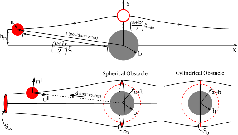
Figure 1: Schematic representation of the problem. (top) The small circle of radius $a$ on the left represents the moving sphere, with a corresponding incoming impact parameter $b_{in}$. The circle of radius $b$ with its centre at the origin of coordinates represents the fixed obstacle (either a sphere or a cylinder). The empty circle represents the position of the suspended particle as it crosses the symmetry plane normal to the $x$ axis. The surface-to-surface separation $\xi$ and its minimum value $\xi_{min}$ are also shown. (bottom) Representation of the conservation argument used to calculate the minimum separation (see §4). The unit vector in the radial direction $\mathbf{d}$ is shown, as well as the velocity components in the plane of motion. The surfaces over which the flux is conserved are shown, both far upstream ($S_{\infty}$) and at the plane of symmetry ($S_{0}$). The geometry is shown for the cases of a spherical and a cylindrical obstacle as indicated.

2.2 Mobility functions for the problem

In Stokes flows, the velocity of the suspended particle $\mathbf{U}$ is linear in the driving field $\boldsymbol{\mathcal{F}}$, such that $\mathbf{U}=\mathsfbi{M}~{}\boldsymbol{\cdot~{}\mathcal{F}}$ for an appropriate mobility tensor $\mathsfbi{M}$ that depends on the geometry of the particle-obstacle system. Moreover, since the particle motion is contained in the $xy$-plane, the velocity can be decomposed into two mutually orthogonal components in that plane; a radial component along $\mathbf{d}$ and a tangential component perpendicular to it (Batchelor, 1982; Davis & Hill, 1992). Then, given the symmetries of the system, the particle velocity can be represented as,

$$\mathbf{U}=(A(r)\mathbf{dd}+B(r)(\boldsymbol{\delta}-\mathbf{dd}))\cdot\boldsymbol{\mathcal{F}},$$ (1)

where $\boldsymbol{\delta}$ is the identity dyadic, and $A$ and $B$ are scalar functions of the separation $r$ (or equivalently, $\xi$), and also depend on the aspect ratio $\beta=b/a$.

It is well known that no analytical expressions are available for the radial ($A$) and tangential ($B$) mobility functions that are valid throughout the entire range of separations ($r\in\left(a+b,\infty\right)$ or $\xi\in\left(0,\infty\right)$). Instead, it is a common practice to derive expressions in two limiting cases, the near-field ($\xi\ll 1$) and the far-field ($\xi\gg 1$) limits (Jeffrey & Onishi, 1984; Kim & Karrila, 1991), and use some matching or interpolation procedure for intermediate separations. Lubrication theory and multipole expansions (equivalently, Lamb’s general solution, method of reflections) are typically employed to derive mobility functions in the near-field and far-field, respectively. Available results in these limiting cases are briefly discussed below, as it will be useful for subsequent derivations. A more detailed discussion of the mobility functions used in this work is presented in appendix A.

2.3 Mobility functions near contact $(\xi\ll 1)$

For sufficiently small separations, lubrication theory yields the following functional forms for the leading order of the radial and tangential mobility functions:

$$A(\xi) \approx a_{0}\xi,$$ (2)

$$B(\xi) \approx\frac{b_{1}}{\ln(1/\xi)}.$$ (3)

Expressions are available for the coefficients $a_{0}$ and $b_{1}$ above, for any generic pair of convex surfaces that can be approximated by a quadratic form (Cox, 1974; Claeys & Brady, 1989). In particular, Kim & Karrila (1991) provide the following expressions for $a_{0}$ and $b_{1}$ for a pair of spheres:

$$a_{0} =\frac{k_{0}}{6\math@atom{\pi}{\mathchoice{\hbox{$\displaystyle\pi$}}{\hbox{$\textstyle\pi$}}{\hbox{$\scriptstyle\pi$}}{\hbox{$\scriptscriptstyle\pi$}}}\mu a}\left[\frac{\beta}{2}\left(1+\frac{1}{\beta}\right)^{3}\right],$$

$$b_{1} =\frac{k_{1}}{6\math@atom{\pi}{\mathchoice{\hbox{$\displaystyle\pi$}}{\hbox{$\textstyle\pi$}}{\hbox{$\scriptstyle\pi$}}{\hbox{$\scriptscriptstyle\pi$}}}\mu a}\left[2\left(1+\frac{1}{\beta}\right)^{3}\right],$$

where, the constants $k_{i}=1$ for the case of a constant force acting on the particle, but are functions of $\beta$ in the case of a uniform velocity driving the particle. They can be written in terms of the $O(1)$-terms of the respective resistance functions, using the notation due to Kim & Karrila (1991):

$$k_{0} =A^{X}_{11}+\frac{1}{2}\left(1+\beta\right)A^{X}_{12},$$

$$k_{1} =A^{Y}_{11}+\frac{1}{2}\left(1+\beta\right)A^{Y}_{12}+\frac{1}{6}\frac{\beta+4}{\beta+1}\left(B^{Y}_{11}+\frac{1}{4}\left(1+\beta\right)^{2}B^{Y}_{12}\right).$$

The numerical values of $k_{i}$ for various values of $\beta$ are tabulated in Appendix A.

Nitsche (1996) applies expressions derived by Claeys & Brady (1989) to the case of a sphere moving relative to a cylinder of the same radius, in the case of a constant force driving the particle. We apply the same expressions to arbitrary ratios of radii to obtain:

$$a_{0} =\frac{1}{6\math@atom{\pi}{\mathchoice{\hbox{$\displaystyle\pi$}}{\hbox{$\textstyle\pi$}}{\hbox{$\scriptstyle\pi$}}{\hbox{$\scriptscriptstyle\pi$}}}\mu a}\left[\frac{1+2\beta}{4}\left(1+\frac{1}{\beta}\right)^{3/2}\right],$$

$$b_{1} =\frac{1}{6\math@atom{\pi}{\mathchoice{\hbox{$\displaystyle\pi$}}{\hbox{$\textstyle\pi$}}{\hbox{$\scriptstyle\pi$}}{\hbox{$\scriptscriptstyle\pi$}}}\mu a}\left[3\left(1+\frac{1}{\beta}\right)^{1/2}\right].$$

2.4 Mobility functions at large separations $(\xi\gg 1)$

In the case of a constant force driving the particle past a spherical obstacle, we use the far-field expansions of the mobility functions provided by Kim & Karrila (1991) to obtain the following expressions for the functions $A(r)$ and $B(r)$ in powers of $(a/r)$:

$$A(r) =\frac{1}{6\math@atom{\pi}{\mathchoice{\hbox{$\displaystyle\pi$}}{\hbox{$\textstyle\pi$}}{\hbox{$\scriptstyle\pi$}}{\hbox{$\scriptscriptstyle\pi$}}}\mu a}\left[1-\frac{9}{4}\beta\left(\frac{a}{r}\right)^{2}+\left(\frac{3\beta}{2}-\frac{9\beta^{3}}{4}\right)\left(\frac{a}{r}\right)^{4}+O\left(\frac{1}{r^{6}}\right)\right],$$

$$B(r) =\frac{1}{6\math@atom{\pi}{\mathchoice{\hbox{$\displaystyle\pi$}}{\hbox{$\textstyle\pi$}}{\hbox{$\scriptstyle\pi$}}{\hbox{$\scriptscriptstyle\pi$}}}\mu a}\left[1-\frac{9}{16}\beta\left(\frac{a}{r}\right)^{2}-\frac{3}{8}\left(\beta+3\beta^{3}\right)\left(\frac{a}{r}\right)^{4}+O\left(\frac{1}{r^{6}}\right)\right].$$

Analogously, in the case of a uniform velocity field and a spherical obstacle we obtain,

$$A(r) =\frac{1}{6\math@atom{\pi}{\mathchoice{\hbox{$\displaystyle\pi$}}{\hbox{$\textstyle\pi$}}{\hbox{$\scriptstyle\pi$}}{\hbox{$\scriptscriptstyle\pi$}}}\mu a}\left[1-\frac{3\beta}{2}\left(\frac{a}{r}\right)+\frac{1}{2}\left(\beta+\beta^{3}\right)\left(\frac{a}{r}\right)^{3}+O\left(\frac{1}{r^{5}}\right)\right],$$

$$B(r) =\frac{1}{6\math@atom{\pi}{\mathchoice{\hbox{$\displaystyle\pi$}}{\hbox{$\textstyle\pi$}}{\hbox{$\scriptstyle\pi$}}{\hbox{$\scriptscriptstyle\pi$}}}\mu a}\left[1-\frac{3\beta}{4}\left(\frac{a}{r}\right)-\frac{1}{4}\left(\beta+\beta^{3}\right)\left(\frac{a}{r}\right)^{3}+O\left(\frac{1}{r^{5}}\right)\right].$$

Note that, the leading order terms in the limit $a\ll b$ describe the streamlines of a uniform flow past a fixed spherical obstacle.

Finally, in the case of a constant force acting on a sphere moving past a cylindrical obstacle we use the following empirical far-field forms for radial and tangential mobility functions proposed by Nitsche (1996):

$$A(r) =\frac{1}{6\math@atom{\pi}{\mathchoice{\hbox{$\displaystyle\pi$}}{\hbox{$\textstyle\pi$}}{\hbox{$\scriptstyle\pi$}}{\hbox{$\scriptscriptstyle\pi$}}}\mu a}\left(1-\frac{117\math@atom{\pi}{\mathchoice{\hbox{$\displaystyle\pi$}}{\hbox{$\textstyle\pi$}}{\hbox{$\scriptstyle\pi$}}{\hbox{$\scriptscriptstyle\pi$}}}}{128}\frac{a/r}{\ln(r/a\beta)+2.39}\right),$$ (4)

$$B(r) =\frac{1}{6\math@atom{\pi}{\mathchoice{\hbox{$\displaystyle\pi$}}{\hbox{$\textstyle\pi$}}{\hbox{$\scriptstyle\pi$}}{\hbox{$\scriptscriptstyle\pi$}}}\mu a}\left(1-\frac{48\math@atom{\pi}{\mathchoice{\hbox{$\displaystyle\pi$}}{\hbox{$\textstyle\pi$}}{\hbox{$\scriptstyle\pi$}}{\hbox{$\scriptscriptstyle\pi$}}}}{128}\frac{a/r}{\ln(r/a\beta)+3.39}\right).$$ (5)

Here, we do not consider the case of a uniform velocity field driving a particle past an unbounded cylinder, since in this case, the description of the far-field motion in terms of mobility functions is not possible due to Stokes’ paradox (Happel & Brenner, 1965). In practice, however, the motion of the particle far from the obstacle would probably be dictated by the physical boundaries of the system (e.g. the walls of the microfluidic device). A similar ‘screening’ argument will become relevant when we discuss the far-field asymptotic probability distribution in §3.2. In order to understand the role of confinement, we shall consider the motion of a particle past a cylindrical obstacle between two parallel walls forming a channel of width $2\ell_{0}$. We shall assume that the particle moves in the mid-plane, driven by a constant force and thus the far-field mobility is dictated by the hydrodynamic interaction with the channel walls (Happel & Brenner, 1965):

$$M_{wall}(r)=\frac{1}{6\pi\mu a}\left[1-1.004\left(\frac{a}{\ell_{0}}\right)+0.418\left(\frac{a}{\ell_{0}}\right)^{3}+0.21\left(\frac{a}{\ell_{0}}\right)^{4}-0.169\left(\frac{a}{\ell_{0}}\right)^{5}\right]$$

As explained in appendix A, at intermediate separations we interpolate between this far-field mobility and the mobility of a sphere in the vicinity of an infinite cylinder. The latter is obtained by an interpolation between (4) (or (5)) and the lubrication regime discussed in §2.3 (Nitsche, 1996).

3 Steady-state distribution of particles around a fixed obstacle

From an Eulerian point-of-view, we are interested in the steady-state distribution of particles around a fixed obstacle. The basic assumption in this investigation is that the particles are uniformly distributed far away from the obstacle, leading to a uniform flux of incoming particles at infinity. The probability density of finding a particle at a given position $\mathbf{r}$ from the obstacle centre (i.e., the origin) is then analogous to the pair distribution function studied in dilute suspensions (Batchelor & Green, 1972; Batchelor, 1982; Davis & Hill, 1992; Almog & Brenner, 1997). Thus, we talk of the pair distribution function $p(\mathbf{r},t)$, referring to particle-obstacle pairs, with the fixed obstacle located at the origin and the particle at position $\mathbf{r}$. Further, $p({\bf r},t)$ is the normalised distribution function, such that the actual probability density is given by $n_{p}p({\bf r},t)$, where $n_{p}$ is the uniform number density of particles far from the obstacle.

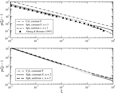
Figure 2: Excess probability distribution ($p(\xi)-1$) as a function of the dimensionless surface-to-surface separation, for radius-ratio $\beta=1$. (top) Comparison between both flow cases for a spherical obstacle with $n=3$ and a cylindrical obstacle. (bottom) Comparison between both flow cases for a spherical obstacle with $n=2$ and a cylindrical obstacle.

Following Batchelor & Green (1972), we start with the conservation equation for the number of particles, which in terms of the pair distribution function can be written as follows:

$$\frac{dp}{dt}=\frac{\partial p}{\partial t}+{\mathbf{U}}\cdot\nabla p=-p\nabla\cdot{\mathbf{U}}.$$ (6)

Then, we write the divergence of the particle velocity in terms of its radial component using (1),

$$\nabla\cdot{\mathbf{U}}=\left[\frac{(n-1)(A-B)}{rA}+\frac{1}{A}\frac{dA}{dr}\right]U_{r},$$ (7)

where $n$ equals $2$ or $3$ depending on the dimensionality of the problem (see the discussion below). Substituting this expression into (6) we obtain,

$$\frac{dp}{dt}=-pU_{r}\left[\frac{(n-1)(A-B)}{rA}+\frac{1}{A}\frac{dA}{dr}\right]=pU_{r}\frac{1}{q}\frac{dq}{dr}=p\frac{dr}{dt}\frac{1}{q}\frac{dq}{dr}=\frac{p}{q}\frac{dq}{dt},$$ (8)

where, following Batchelor & Green (1972) we introduced a function $q(r)$ defined such that $p(\mathbf{r},t)/q(r)$ is a constant of motion (its material derivative is zero). This result is valid for both types of obstacles and both driving fields, with $q(r)$ determined by the mobility functions specific to each case. Further, $p(\mathbf{r},t)/q(r)$ is constant under both steady as well as unsteady conditions and, as a result, the distribution of particles at a position $\mathbf{r}$ and time $t$ can be determined from a previous position of the same material point at a prior time. In addition, in steady state $p(\mathbf{r})/q(r)$ is constant along trajectories, which implies a stationary, radially symmetric distribution of particles (i.e., $p(\mathbf{r})\equiv p(r)$), a surprising result, but one that is analogous to that obtained by Batchelor & Green (1972). An alternative way to arrive at the same result is to propose a function $q(r)$ such that the field $q\mathbf{U}$ becomes solenoidal and therefore $p/q$ is constant along particle trajectories. We can obtain a solenoidal field by multiplying the velocity with a function $q$ of the magnitude $r$ only, which indicates an isotropic distribution of particles in steady state. Finally, solving for $q(r)$ and imposing the asymptotic limit $p(r\to\infty)\to 1$, we obtain a general expression for the pair distribution function in terms of the mobility functions A and B,

$$p(r)=\frac{A^{\infty}}{A(r)}\exp\left\{\displaystyle\int_{r}^{\infty}\frac{(n-1)(A-B)}{rA}dr\right\},$$ (9)

where $A^{\infty}=1/(6\pi\mu a)$ is the asymptotic value of the radial mobility function for $r\to\infty$. The precise effect of geometry and driving field is captured by the hydrodynamic mobility functions $A$ and $B$, as well as the effective dimensionality $n$ of the problem. An infinitely long cylindrical obstacle naturally imposes a two dimensional geometry ($n=2$). However, there are two independent possibilities in the case of a spherical obstacle. First, the fully 3-dimensional (3D) problem of a dilute suspension moving past a spherical obstacle corresponds to $n=3$. The second problem corresponds to the case in which the suspended particles are restricted to move in the $xy$-plane, i.e., the plane of the paper in figure 1. This simplification corresponds to $n=2$, and is sometimes used to approximate the motion past a cylindrical fibre (Phillips et al., 1989, 1990).

In figure 2, we show the probability density function for an aspect ratio $\beta=1$ and various possibilities in terms of driving field, geometry of the obstacle, and the associated dimensionality. The top plot shows that the distribution of particles around a cylindrical obstacle is almost five-fold larger than that in the case of a spherical obstacle with $n=3$ for a given separation from the obstacle. The distribution is observed to be less sensitive to the effect of the driving field (spherical obstacle, $n=3$), with that for the particles driven by a constant force being higher than when they are driven by a uniform velocity field. The same plot also shows a good agreement between our calculations for a spherical obstacle (with $n=3$) and those of Almog & Brenner (1997), for the case of a particle driven by a uniform velocity field. Note that, Almog & Brenner (1997) have analysed the equivalent case of a particle moving with a prescribed constant velocity in a suspension of neutrally buoyant spheres. In the bottom plot we compare the probability distribution around a cylindrical obstacle with that around a spherical obstacle when the incoming particles are restricted to move in the $xy$-plane ($n=2$). The distributions exhibit similar behaviour at small separations. However, we will show that the asymptotic scaling of the probability distributions in the limit of small separations is different for each geometry of the obstacle. We also note that all the distributions are in fact divergent at contact ($\xi\to 0$). We shall discuss the asymptotic behaviour and this divergence of the probability distributions in more detail in §3.1.

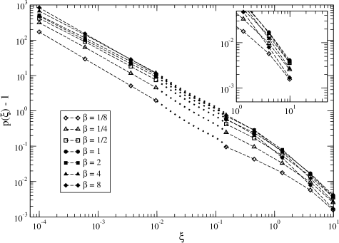
Figure 3: Excess probability distribution ($p(\xi)-1$) as a function of dimensionless surface-to-surface separation, for different aspect ratios $\beta$, a constant force and a spherical obstacle ($n=3$). Inset: Enlarged view for large values of $\xi$, depicting symmetric behaviour about $\beta=1$ for a fixed value of $\xi$, i.e., filled and open symbols almost overlap.

In figure 3, we compare the probability distribution function for different aspect ratios between the suspended particle and a spherical obstacle at the centre ($n=3$) when the particle is driven by a constant force. The distribution of particles increases monotonically with the aspect ratio $\beta$ for relatively small separations, $\xi\lesssim 1$. However, for large separations the probability distribution function exhibits a symmetric scaling behaviour with respect to the aspect ratio, in that the same leading order expressions are obtained for $\beta$ and $\beta^{-1}$, as discussed in §3.2 below.

As mentioned before, the mobility functions used to calculate the probability distribution plotted in figures 2 and 3 in the case of a spherical obstacle were obtained from the literature for the limiting cases of small and large separations. For intermediate separations, a transition is made between the two limits using interpolation. This interpolation region is depicted by dotted lines in figures 2 and 3. For the cylindrical obstacle, we have used interpolated functions empirically computed by Nitsche (1996) over the entire range of separations (see Appendix A).

3.1 Asymptotic behaviour of the probability distribution near contact

In order to investigate the asymptotic behaviour of the probability distribution near contact, we first rewrite (9) in terms of the dimensionless surface-to-surface separation $\xi$,

$$p(\xi)=\frac{A^{\infty}}{A(\xi)}\exp\left\{(n-1)H(\xi)\right\},$$ (10)

where,

$$H(\xi)=\displaystyle\int_{\xi}^{\infty}\frac{(A-B)}{2\left(1+\frac{\tilde{\xi}}{2}\right)A}d\tilde{\xi}.$$ (11)

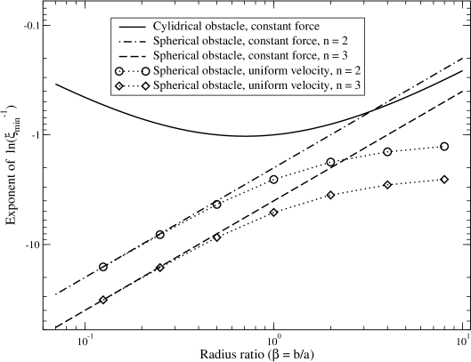
Figure 4: Exponents of $\ln(\xi^{-1}_{min})$ from (12), (22) and (24) as a function of $\beta$ for both cylindrical and spherical obstacles. The exponent for the case of a uniform velocity driving a particle past a sphere ($\Diamond$ and $\bigcirc$) is evaluated at discrete values of $\beta=1/8,~{}1/4,~{}1/2,~{}1,~{}2,~{}4,~{}8$, as explained in the text.

For small separations, we can split the domain of integration for $H(\xi)$ at some arbitrary value $\xi_{0}\ll 1$ such that the expressions for the mobility functions $A$ and $B$ can be approximated using lubrication theory in the near-field part of the integral, where $\xi\ll 1$. From this lubrication region we obtain the leading order term for the probability distribution of particles at small separations,

$$p(\xi)\approx p_{0}\xi^{-1}(\ln(\xi^{-1}))^{-(n-1)\alpha}~{}~{}~{}\ldots~{}\alpha=\frac{b_{1}}{2a_{0}}~{},$$ (12)

where $p_{0}$ is a constant that depends on the geometry and driving field, and from §2.3, $\alpha=2k_{1}/k_{0}\beta$ for the case of a spherical obstacle, while $\alpha=6\beta(1+2\beta)^{-1}(1+\beta)^{-1}$ for the case of a constant force driving the particle past a cylindrical obstacle. The divergence of the probability distribution at small separations is dominated by the $\xi^{-1}$ term, which explains the apparent linear behaviour observed in figure 2 and the weak dependence on the aspect ratio observed in figure 3. The asymptotic expression (12) is similar to the results obtained by Batchelor (1982) and Khair & Brady (2006). They obtain an expression of the form $p(\xi)\sim\xi^{-\ell}(\ln(\xi^{-1}))^{-m}$, wherein $\ell(\neq 1)$ arises due to the presence of $O(\xi^{0})$ terms in their tangential mobility functions. These terms are exactly zero when the obstacle is fixed, leading to $\ell=1$, as obtained in (12). Figure 4 shows the exponent $-(n-1)\alpha$ in the equation above, as a function of $\beta$ for both types of obstacles. As mentioned in §2.3, $k_{1}=k_{0}=1$ for the case of a constant force driving the particle past a spherical obstacle. This leads to $\alpha=2/\beta$, corresponding to the two straight lines in the log-log plot presented in the figure. Further, for the case of a uniform velocity driving the particle, $k_{0}$ and $k_{1}$ can be computed using the numerical values of the $O(1)$ terms in the corresponding resistance functions, which are available at discrete values of the aspect ratio (Jeffrey & Onishi, 1984; Kim & Karrila, 1991). This leads to a numerical evaluation of the exponent at these values, as shown in the figure (see appendix A for a table of values of $k_{0}$ and $k_{1}$). We note that for very small values of the aspect ratio$\beta$ – i.e., when the obstacle is very small compared to the particle – we get $k_{0}\approx k_{1}\approx 1$, and the exponent for the case of a spherical obstacle becomes equal for both types of driving fields. This is consistent with a constant drag acting on the suspended particle outside the lubrication region.

Finally, we note the presence of a diffusive boundary layer around the obstacle. A local Péclet number for the particle, $Pe_{L}$, can be written as the ratio between the radially inward convective flux ($j_{C}=n_{P}p(\xi)U_{r}$) and the radially outward diffusive flux ($j_{D}=-n_{P}Ddp/dr$). At small separations we can use the asymptotic behaviour of $p(\xi)$ to obtain,

$$Pe_{L} =\frac{j_{C}}{j_{D}}=-\frac{n_{P}pU_{r}}{n_{P}Ddp/dr}=-\frac{p(\xi)}{dp/d\xi}\cdot\frac{(a+b)\mathcal{F}}{2kT}\sim~{}\xi Pe_{0},$$

where, $Pe_{0}=(a+b)\mathcal{F}/{2kT}$ is the system Péclet number. This indicates the existence of a boundary layer around the obstacle for $\xi\lesssim 1/Pe_{0}$, within which the diffusive mode of transport dominates over the convective one. Thus, the expressions derived above for the probability distribution, under the deterministic assumption, are not valid within this boundary layer. Batchelor (1982) highlights this issue for sedimenting suspensions. Nitsche (1996) discusses the presence of such a boundary layer in the context of the diffusion of a spherical particle close to a cylindrical fibre of comparable size and Khair & Brady (2006) have quantified this region in the context of micro-rheology.

3.2 Asymptotic behaviour of the probability distribution at large distances

In order to obtain the leading order behaviour of the probability distribution far from the obstacle, we use the expressions for the far-field mobility functions discussed in §2.4. Substituting these far-field expressions for the mobility functions $A$ and $B$ in (9), we obtain the asymptotic probability distribution for $\xi\gg 1$,

$$p^{F}_{Sph}(r)\sim 1+\frac{45}{32}\beta\left(\frac{a}{r}\right)^{2}+O\left[\left(\frac{a}{r}\right)^{4}\right],$$ (13)

$$p^{v}_{Sph}(r)\sim 1+\frac{3}{4}\beta\frac{a}{r}+\frac{27}{32}\beta^{2}\left(\frac{a}{r}\right)^{2}+O\left[\left(\frac{a}{r}\right)^{3}\right],$$ (14)

$$p^{F}_{Cyl}(r)\sim 1+\frac{1.18(a/r)}{\left(3.39+\ln\left[\frac{r}{a\beta}\right]\right)}+O\left[\left(\frac{a}{r}\right)^{2}\right],$$ (15)

corresponding to a spherical obstacle ($n=2$) and constant driving force, a spherical obstacle ($n=2$) and a uniform velocity field driving the particle, and a cylindrical obstacle and a constant driving force, respectively.

Further, for a spherical obstacle with $n=3$, the following expressions for the asymptotic distribution are obtained:

$$p^{F}_{Sph}(r)\sim 1+\frac{9}{16}\beta\left(\frac{a}{r}\right)^{2}+O\left[\left(\frac{a}{r}\right)^{4}\right],$$ (16)

$$p^{v}_{Sph}(r)\sim 1+\frac{27}{8}\beta^{2}\left(\frac{a}{r}\right)^{5}+O\left[\left(\frac{a}{r}\right)^{6}\right],$$ (17)

Note that both (13) and (16) are symmetric about $\beta=1$ for a given (albeit large) separation $\xi$. This can be observed in figure 3 for $\xi\sim 10$ (see inset). When the particle and the obstacle can be treated as point forces separated far apart, the expressions the for mobility functions (given in §2.4) become symmetric in their radii $a$ and $b$, which leads to the symmetry shown above. In contrast, the mobility functions and the corresponding probability distribution remain asymmetric in the case of a uniform velocity field driving the particles.

Analogous expansions in the case of suspension flows are discussed by Batchelor (1982) and by Almog & Brenner (1997) in the context of micro-rheology. However, there is an important difference with these cases. The expressions for $n=2$, (13), (14) and (15) (for $n=3$, (16)) indicate that the integral $\int_{(a+b)}^{R}[p(r)-1]2\pi rdr$ (correspondingly, $\int_{(a+b)}^{R}[p(r)-1]4\pi r^{2}dr$) diverges for $R\to\infty$. Physically, this integral indicates a divergence in the total excess number of particles in the suspension at steady state, induced by the long-range nature of the hydrodynamic interactions with the fixed obstacle. As we mentioned earlier in §2.4, in the case of microfluidics either the channel walls and/or the presence of other suspended particles would effectively screen such long-range interactions, thus leading to convergent integrals. On the other hand, the asymptotic particle distribution around a spherical obstacle for the case of a uniform velocity field and $n=3$ given by (17), yields a finite excess number of particles. We attribute this to the rapidly decaying divergence of the particle velocity in this case, given by (7, $n=3$),

$$\nabla\cdot{\mathbf{U}}\propto\ln[p(r)]\sim\frac{27}{8}\beta^{2}\left(\frac{a}{r}\right)^{5}~{}~{}~{}\ldots~{}~{}~{}r\gg 1.$$

4 Minimum surface-to-surface separation

We now turn to the dependence of the dimensionless minimum surface-to-surface separation, $\xi_{min}$ (equivalently, the corresponding centre-to-centre separation $r_{min}$), on the incoming impact parameter $b_{in}$, following both Eulerian and Lagrangian approaches. The Eulerian approach entails invoking the conservation of the number of particles entering and exiting the region defined by the revolution of the trajectory of a particle around the $x$-axis (the region created by the translation of a particle trajectory along the axis of the cylinder in the case of a cylindrical obstacle). The Lagrangian approach involves the explicit calculation of the trajectory of an individual particle, followed by the evaluation of the position of the particle as it crosses the plane $x=0$.

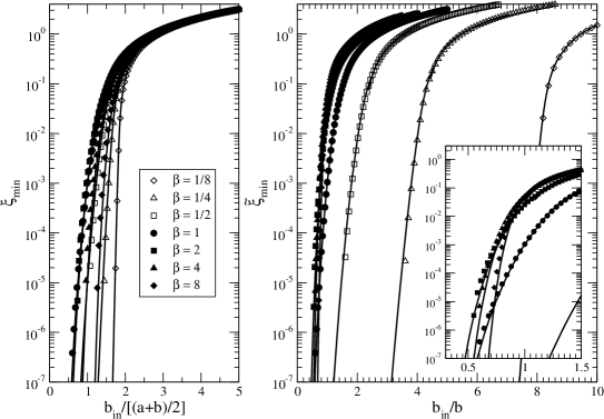
Figure 5: Minimum separation $\xi_{min}$ versus incoming impact parameter $b_{in}$. Comparison between particle-particle simulations (Frechette & Drazer, 2009) and the analytical result given in (20): different symbols depict the simulation data as described in the legend, while the solid lines represent (20). (left) Average radius, $(a+b)/2$, is used to nondimensionalize the axes, (right) radius of the obstacle is used to nondimensionalize the axes, $\tilde{\xi}=[(1+\beta)/2\beta]\xi$, (inset) Enlarged view of the interval $(0.5,1.5)$ of $\tilde{b}_{in}$

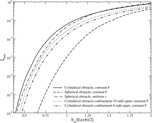
Figure 6: Minimum separation $\xi_{min}$ versus incoming impact parameter $b_{in}$ for different geometries and flow-fields when the particle and the obstacle are of the same radius. The incoming impact parameter is made dimensionless using the average radius, $(a+b)/2$. As explained in the text, for a cylindrical obstacle, the minimum separation decreases for a given incoming impact parameter in case of a confined system.

4.1 Eulerian approach: Conservation of the number of particles

We consider the situation depicted in the bottom half of figure 1. On the left, it shows the volume of revolution obtained by revolving around the axis of motion ($x$-axis) the trajectory followed by a spherical particle moving past a spherical obstacle. The conservation of particles inside this volume of revolution takes a simple form, due to the fact that the flux of particles across the surface of revolution is zero; since trajectories do not cross in Stokes flow. (The construction of such a volume of revolution corresponds to the fully 3D case with $n=3$. The 2D case with $n=2$ can be treated in a manner completely analogous to that of a cylindrical obstacle.) Then, we calculate the flux at two cross sections that are perpendicular to the $x$-axis, and over which the velocity is exactly normal to the surface. These two surfaces are depicted in figure 1: one is the cross section far upstream, indicated by $S_{\infty}$, and the otheris the annular region corresponding to the cross section at $x=0$, indicated by $S_{0}$ in the figure. (Note the excluded volume of radius $(a+b)$). On the bottom right corner of the figure, we show the analogous case of a cylindrical obstacle, in which the flux is considered per unit length in the $z$-direction. In both cases the local flux of particles is given by $p(\mathbf{r})\mathbf{U}$. Therefore, the conservation of particles in terms of surface integrals takes the form,

$$\int_{S_{\infty}}\left.p\mathbf{U}\right|_{x\rightarrow-\infty}\cdot d\mathbf{S}=\displaystyle\int_{S_{\infty}}p_{\infty}\,U_{\infty}\,dS=\displaystyle\int_{S_{0}}p_{0}\,U_{0}\,dS=\displaystyle\int_{S_{0}}\left.p\mathbf{U}\right|_{x=0}\cdot d\mathbf{S},$$ (18)

where $U_{\infty}$ and $U_{0}$ are the magnitude of the particle velocity far upstream and at $x=0$, respectively. The integration over $S_{\infty}$ is simple, the probability distribution tends to unity and the velocity is uniform. Specifically, the velocity is asymptotically radial and equal to $A^{\infty}\mathcal{F}$, that is $F/6\pi\mu a$ or $v^{\infty}$, depending on the driving field. The flux is, therefore, $S_{\infty}A^{\infty}\mathcal{F}$, with $S_{\infty}=\pi^{(n-2)}b^{(n-1)}_{in}$. At the plane of symmetry, the velocity is tangential to the obstacle, $U_{0}=B(r)\mathcal{F}$. Then, substituting in (18) and performing suitable algebraic simplifications we obtain,

$$\frac{b_{in}^{n-1}}{n-1}=\displaystyle\int_{a+b}^{r_{min}}\frac{B(r)}{A(r)}r^{n-2}\exp\left\{\displaystyle\int_{r}^{\infty}\frac{(n-1)(A-B)}{\tilde{r}A}d\tilde{r}\right\}dr,$$ (19)

where the limits of integration of the annular region are the excluded volume radius $(a+b)$ and the radial position of the particle at $x=0$, which corresponds to the minimum radial distance reached during the course of the motion, $r_{min}$. We can simplify the equation further, as shown in Appendix B to yield,

$$b_{in}=r_{min}\exp\left\{H\left(\xi_{min}\right)\right\},$$ (20)

where $H$ is the function defined in (11).

4.2 Lagrangian approach: Trajectory analysis

The differential equation for the particle trajectory in terms of $y$ and $r$ coordinates can be integrated in a straightforward manner by separation of variables,

$$\frac{dy}{dr}=\frac{U_{y}}{U_{r}}=\frac{U_{r}\sin\theta+U_{\theta}\cos\theta}{U_{r}}=\sin\theta-\frac{B(r)\mathcal{F}\sin\theta}{A(r)\mathcal{F}\cos\theta}\cos\theta=y\left[\frac{1}{r}-\frac{B(r)}{r~{}A(r)}\right].$$ (21)

Thus, upon integration between $(y=b_{in},r\to\infty)$ and $(y,r)$ we get,

$$\ln\left(\frac{b_{in}}{y}\right)=\displaystyle\int_{r}^{\infty}\frac{A(r)-B(r)}{rA(r)}dr=H(\xi)\Rightarrow b_{in}=y\exp\{H(\xi)\}.$$

Evaluating at $x=0$ (where $y=r_{min}$ and $\xi=\xi_{min}$), we retrieve (20).

The expression (20) explicitly relates the minimum separation between particle and obstacle surfaces with the incoming impact parameter, and is a general result applicable to systems in which the velocity can be decomposed as in (1). It is interesting to note that it has the same form for the relation between $b_{in}$ and $r_{min}$ (or, $\xi_{min}$) for two and three dimensional geometries, which can be explained by the fact that the motion is planar in both cases. Again, the entire information about the driving field and the geometry of the problem is implicit in the mobility functions $A(r)$ and $B(r)$.

In figure 5, we compare the minimum separation obtained using (20) with that obtained from the numerical integration of the trajectory followed by a spherical particle moving around a fixed spherical obstacle (Frechette & Drazer, 2009). Excellent agreement is observed for all the aspect ratios considered, $\beta=0.125,0.25,0.5,1,2,4,8$. Note that the same mobility functions were used in both cases, hence the agreement is independent of the accuracy of the mobility functions themselves. In order to illustrate (20) in a practical manner, we also present the minimum separation for particles of different size when the size of the obstacle is fixed (see right hand panel in figure 5). We observe that for a constant incoming impact parameter, $b_{in}/b\sim O(1)$, the minimum attained separation decreases with increasing particle radius. However, an asymptotic analysis at very small separations reveals that for a given (sufficiently small) incoming impact parameter, the minimum separation decreases monotonically with decreasing particle radius. This can be corroborated from the behaviour of the exponent involved in the asymptotic scaling of the incoming impact parameter (22) shown in figure 4 (see §4.3 below for a detailed discussion). The inset in the right hand panel of figure 5, in fact, portrays the imminent reversal of this trend in the form of the criss-crossing curves. Figure 6 shows $\xi_{min}$ as a function of $b_{in}$ for $\beta=1$ for five different cases. We can see that for a constant driving force and a given $b_{in}$ the particle gets closer to a spherical obstacle, compared to a cylindrical one. It also shows that a constant force drives the particle closer to a spherical obstacle than a uniform velocity field. Further, we show the case of an obstacle-particle pair confined between two parallel walls, when the obstacle is a cylinder and the walls are perpendicular to the axis of the cylinder. This case is the most relevant to model the motion of a particle past a cylindrical post in a microfluidic channel. As explained in §2.4 and appendix A, at intermediate separations we compute the mobility of the particle in this system by interpolating between the mobility of a sphere moving along the mid-plane between the two walls (Happel & Brenner, 1965) and that for a particle moving close to an infinite cylinder (Nitsche, 1996). We observe that the presence of such confinement, as well as increasing the extent of the confinement from 10 particle radii to 6 particle radii, decreases the attained minimum separation for a given incoming impact parameter. The underlying reason is that, in the far-field, the mobility is isotropic in the plane of motion and, therefore, the motion of the particle is not affected by the obstacle. The interaction with the obstacle becomes significant for particle-obstacle separations of the order of the channel width. Thus, for a narrower channel, the particle reaches closer to the obstacle before its mobility is affected by the presence of the obstacle. The minimum separation attained by the particle along its trajectory determines the relevance of short-ranged repulsive forces during its motion. Thus, in terms of the effect of confinement, the above observation implies that the particle will experience an earlier onset of non-hydrodynamic effects upon confinement between two parallel walls.

4.3 Asymptotic behaviour of minimum separation near contact, $\xi_{min}\to 0$

Here, we calculate the asymptotic behaviour of the relation (20) in the limit of very small separations, in a manner similar to that discussed in §3.1 for the probability distribution. Specifically, using the lubrication approximation for the mobility functions in §2.3, and substituting in (20) we get:

$$\left(\frac{b_{in}}{(a+b)/2}\right)\approx\lambda_{0}(\ln(1/\xi_{min}))^{-\alpha}~{}~{}~{}\ldots~{}\alpha=\frac{b_{1}}{2a_{0}},$$ (22)

where $\lambda_{0}$ is a constant that incorporates the contributions from the far-field. The behaviour of the exponent $(-\alpha)$ is depicted in figure 4. As discussed earlier, we can see from the behaviour of the exponent that for incoming imapct parameters small enough to follow (22), the minimum separation decreases monotonically with decreasing particle radius.

However, the asymptotic form of the tangential resistance function $1/B(r)$, derived using (3), is only logarithmically divergent, and valid only when extremely small separations are attained. Thus, for reasonably small values of $\xi_{min}$, albeit $\xi_{min}\ll 1$, the expression (22) is not an accurate approximation. Therefore, in addition to the leading order of the scalar resistance functions from which $B(\xi)$ is obtained by matrix inversion, we also retain their $O(1)$ terms. Consequently, the tangential mobility function takes the form:

$$B(\xi)\approx\frac{1}{6\math@atom{\pi}{\mathchoice{\hbox{$\displaystyle\pi$}}{\hbox{$\textstyle\pi$}}{\hbox{$\scriptstyle\pi$}}{\hbox{$\scriptscriptstyle\pi$}}}\mu a}\frac{s(\xi)(b_{1}+b_{2}s(\xi))}{1+b_{3}s(\xi)+b_{4}s(\xi)^{2}}~{}~{}~{}\ldots~{}~{}~{}s(\xi)=\frac{1}{\ln(1/\xi)}~{}.$$ (23)

We continue to use (2) as an approximation for the radial mobility function, so that $A(\xi)\approx a_{0}\xi$. This leads to the following approximate expression for the scaling:

$$\left(\frac{b_{in}}{(a+b)/2}\right)\approx\frac{\lambda_{1}(s(\xi_{min}))^{\alpha}}{\left(\gamma_{1}+s(\xi_{min})\right)^{\alpha-\gamma_{0}}\left(\gamma_{2}+s(\xi_{min})\right)^{\gamma_{0}}},$$ (24)

where, as before, the exponent $\alpha$ is as defined in (12) and (22), and the constant $\lambda_{1}$ captures the far-field behaviour. The constants $\gamma_{i}$ are functions of the coefficients $b_{i}$ in the tangential mobility function (see appendix A for their tabulated values). In figure 7, we compare the limiting behaviour given by (24), with $\lambda_{1}$ as the only fitting parameter, with the numerical evaluation of the governing relation (20), and observe that there is excellent agreement over a considerable range of separations.

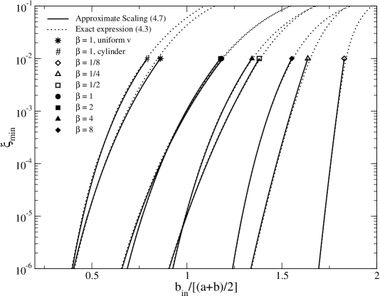
Figure 7: Open and filled symbols represent approximate scaling (24) compared with full governing relation (20) when a particle is driven by a constant driving force past a spherical obstacle for radius-ratios $\beta=1/8,~{}1/4,~{}1/2,~{}1,~{}2,~{}4$ and $8$. (#) represents a particle being driven past a cylindrical obstacle by a constant force, and (*) represents a particle being driven by a uniform velocity field past a spherical obstacle, for $\beta=1$. The multiplicative constant $\lambda_{1}$ is determined by fitting the data generated with (20) for small values of $\xi$. The fitted values are $1.91,~{}1.88,~{}1.84,~{}1.86,~{}1.99,~{}2.33,~{}2.08$ for $\beta=1/8,~{}1/4,~{}1/2,~{}1,~{}2,~{}4,~{}8$, respectively, in the case of the open and filled symbols. For a cylindrical obstacle (#) we obtained $\lambda_{1}=1.58$ and for the case of uniform flow (*) $\lambda_{1}=1.50$.

5 Discussion and Summary

Using (20) it is straightforward to extend the concept of hydrodynamic surface roughness (henceforth, HR) of spheres introduced by Smart & Leighton (1989), to the motion of a suspended particle past a fixed obstacle. In their original work, Smart & Leighton (1989) related the time taken by a sphere to fall away from a flat surface under the action of gravity to an effective surface roughness. In our case, we can establish a relationship between the net lateral displacement experienced by a suspended sphere moving past an obstacle and the length scale at which surface roughness effects become dominant over hydrodynamic forces. This relationship is based on the simple but useful excluded-annulus model in which the inter-particle potential is approximated by a hard sphere repulsion with range $(1+\epsilon)a$ (Brady & Morris, 1997). In this approximation, the effective roughness determines the minimum separation between particles but has no effect on the hydrodynamic interaction between them. Such hard sphere potentials (in some cases including tangential friction) are widely used to model roughness effects on suspension properties, including micro-structure (Rampall et al., 1997; Brady & Morris, 1997; Drazer et al., 2004; Blanc et al., 2011), shear-induced dispersion (da Cunha & Hinch, 1996; Drazer et al., 2002; Ingber et al., 2008), sedimentation (Davis, 1992; Davis et al., 2003), rheology (Wilson & Davis, 2000; Bergenholtz et al., 2002), and transport in periodic systems (Frechette & Drazer, 2009). In our problem, the excluded annulus model implies that, independent of the impact parameter $b_{in}$, separations smaller than $a\epsilon$ are unattainable due to the hard sphere potential. On the other hand, the repulsive potential has no effect as the particle separates from the obstacle. Therefore, if $b_{in}=b_{\epsilon}$ is the incoming impact parameter corresponding to $\xi_{min}=\epsilon$, any trajectory with $b_{in}<b_{\epsilon}$ reaches the same minimum separation $\epsilon$ and collapses onto the outgoing trajectory corresponding to $b_{in}=b_{\epsilon}$, thus inducing a net lateral displacement of magnitude $b_{in}-b_{\epsilon}$. In the case of a dilute suspension flowing past a fixed obstacle, this corresponds to the presence of a wake of width $2b_{\epsilon}$ behind the obstacle, analogous to that observed by Khair & Brady (2006). The excluded-annulus model implies that the wake behind a fixed obstacle is related to the HR by (20),

$$b_{\epsilon}=\left(a+b\right)\left(1+\frac{\epsilon}{2}\right)\exp\left\{H\left(\epsilon\right)\right\}.$$ (25)

Alternatively, we can view the equation above as the definition of the HR, which serves as an effective hard-wall potential resulting from all non-hydrodynamic short-range repulsive interactions. The experimental measurement of $b_{\epsilon}$ would yield such length scale $\epsilon a$ for deterministic systems with negligible particle and fluid inertia. A similar surface characterization method has been employed in the case of colloidal particles by numerically solving the particle trajectories (Dabroś & van de Ven, 1992; van de Ven et al., 1994; Wu & van de Ven, 1996; van de Ven & Wu, 1999; Whittle et al., 2000). We note, however, that due to the presence of a diffusive boundary layer (see §3.1), (25) is valid for sufficiently large Péclet numbers, such that the thickness of the boundary layer is smaller than the repulsive core, i.e., $\xi_{BL}\sim 1/Pe<\epsilon$.

In summary, we have investigated the problem of a spherical, non-Brownian particle negotiating a spherical or cylindrical obstacle in the absence of particle and fluid inertia. The particle is driven by a uniform ambient velocity field or a constant force acting on it, and its motion is entirely contained in the plane formed by the driving force and the radial vector joining the centres of the obstacle and the particle. Given this planar nature of the motion and the symmetry of the problem, the particle velocity renders itself for decomposition into a radial component (along the centre-to-centre line) and a tangential component (perpendicular to the centre-to-centre line), with the corresponding mobility functions being dependent on the centre-to-centre distance only. Based on these properties, and extending an approach introduced by Batchelor & Green (1972) in the context of sheared suspensions, we have derived the steady-state probability distribution of particles around the obstacle, assuming a uniform distribution of incoming particles at infinity. We showed the distribution to be radially symmetric for both obstacle types and both driving fields, analogous to the isotropic pair distribution functions obtained in sheared suspensions, sedimentation and microrheology. The asymptotic form of the distribution funtions diverges at contact, suggesting the presence of a boundary layer around the obstacle in which Brownian transport is not negligible; existence of such a boundary layer has also been reported in the context of sedimenting suspensions and microrheology (Batchelor, 1982; Nitsche, 1996; Khair & Brady, 2006). In addition, the asymptotic distribution of particles close to the obstacle is similar for both driving fields, and depends only weakly on the dimensionality and geometry of the problem. Further, our numerical results indicate that this asymptotic behaviour becomes dominant at small separations, highilighting the relevance of other (non-hydrodynamic) interactions. The other asymptotic limit, that of large separations, yields a divergent excess number of particles around the obstacle, suggesting that screening by other particles or container walls would eventually become important for the description of the distribution of particles far from the obstacle.

We have also derived an expression for the minimum particle-obstacle separation attained in the course of motion, as a function of the incoming impact parameter, using both Eulerian and Lagrangian approaches. We have shown that a smaller minimum separation is attained by particles moving in a confined channel, and the separation decreases with the extent of the confinement. The asymptotic behaviour in the limit of small impact parameters (particles nearly touching the obstacle) shows that the minimum surface-to-surface separation decays exponentially (with a negative power of the impact parameter). The exponent governing this asymptotic relationship varies monotonically with particle radius, and indicates that for a given obstacle size and sufficiently small incoming impact parameter, a smaller particle reaches closer to the obstacle than a larger one. Further, the exponential nature of the relationship shows that extremely small surface-to-surface separations can be frequently encountered in the motion of particles through an array of obstacles, which, could easily lead to a dominant role of non-hydrodynamic interactions in microfluidic systems. Interestingly, the exponential decay of the minimum separation as a function of the impact parameter is independent of the dimensionality of the problem and depends only weakly on the geometry of the obstacle and aspect ratio.

Appendix A Mobility fuctions $A$ and $B$

In this appendix, we describe the radial, $A(r)$, and tangential, $B(r)$, mobility functions used in this work. We also provide the tabulated values of the different coefficients used in the expressions provided for the mobility functions at small surface-to-surface separations.

A.1 Spherical obstacle

In the case of a spherical obstacle we follow the notation used by Jeffrey & Onishi (1984) and write $A$ and $B$ in terms of the scalar functions $x^{a}_{\alpha\beta}$, $x^{b}_{\alpha\beta}$, $x^{c}_{\alpha\beta}$, $y^{a}_{\alpha\beta}$, $y^{b}_{\alpha\beta}$ and $y^{c}_{\alpha\beta}$. The subscript $\alpha\beta$ denotes a function relating the motion of sphere $\alpha$ to the force or torque acting on sphere $\beta$. Consequently the values of $\alpha$ and $\beta$ can be $1$ or $2$. In our case, we use $1$ for the moving particle and $2$ for the obstacle. The expressions for $A$ and $B$ are given below for both driving fields. The near-field and far-field approximations presented in 2.3 and 2.4, respectively, were obtained from the equations below using the expressions tabulated by Kim & Karrila (1991).

A.1.1 Constant force acting on the moving sphere

$$A=\frac{1}{\mu}\left(\frac{-x^{a}_{12}x^{a}_{21}+x^{a}_{11}x^{a}_{22}}{x^{a}_{22}}\right)$$ (26)

$$B=-\frac{1}{\mu}\left(-y^{a}_{11}-y^{a}_{12}\frac{y^{a}_{21}y^{c}_{22}-y^{b}_{21}y^{b}_{22}}{-y^{a}_{22}y^{c}_{22}+(y^{b}_{22})^{2}}+\frac{y^{a}_{21}y^{b}_{21}}{y^{b}_{22}}+\frac{y^{a}_{22}y^{b}_{21}}{y^{b}_{22}}\frac{y^{a}_{21}y^{c}_{22}-y^{b}_{21}y^{b}_{22}}{-y^{a}_{22}y^{c}_{22}+(y^{b}_{22})^{2}}\right)$$ (27)

In table 1 below, we provide the numerical values of the coefficients $b_{i}$ and $\gamma_{i}$ used in §4.3 for the case of a constant force driving the particle:

$\beta$	$b_{1}$	$b_{2}$	$b_{3}$	$b_{4}$	$\gamma_{0}$	$\gamma_{1}$	$\gamma_{2}$
1/8	1458	31574.8	3115.50	31260.7	0.05991	0.00032	0.09934
1/4	250	2900	504.485	2917.17	0.09334	0.00200	0.17093
1/2	54	343.805	102.275	348.493	0.11920	0.01013	0.28335
1	16	56.2240	28.5301	54.6052	0.11890	0.03778	0.48470
2	6.75	12.2487	10.7917	9.67405	0.09389	0.10199	1.01354
4	3.90625	2.55981	4.69405	0.45347	0.06189	0.21761	10.1337
8	2.84766	-0.7352	1.64041	-1.6223	0.21398	1.4394	0.42824

Table 1.  Coefficients $b_{i}$ and $\gamma_{i}$ from (23) and (24). Constant force. Spherical obstacle.

A.1.2 A freely suspended sphere in a uniform ambient velocity field

$$A=\frac{1}{6\pi\mu a}\left(1-\frac{x^{a}_{12}}{x^{a}_{22}}\right)$$ (28)

$$B=\frac{1}{6\pi\mu a}\left(1-\frac{y^{b}_{21}}{y^{b}_{22}}+\frac{y^{a}_{22}y^{b}_{21}-y^{a}_{12}y^{b}_{22}}{y^{b}_{22}}\frac{y^{c}_{22}}{y^{a}_{22}y^{c}_{22}-(y^{b}_{22})^{2}}\right)$$ (29)

In table 2, we enlist the values of the coefficients $b_{i}$ and $\gamma_{i}$ used in §4.3 when a freely suspended particle is driven by a uniform velocity field:

$\beta$	$b_{1}$	$b_{2}$	$b_{3}$	$b_{4}$	$\gamma_{0}$	$\gamma_{1}$	$\gamma_{2}$
1/8	1452.41	31453.9	3115.50	31260.7	0.06001	0.00032	0.09934
1/4	245.43	2847	504.485	2917.17	0.09485	0.00200	0.17093
1/2	50.43	321.072	102.275	348.493	0.1285	0.01013	0.28335
1	13.18	46.299	28.5301	54.6052	0.1518	0.03778	0.48470
2	4.363	7.918	10.7917	9.67405	0.1664	0.10199	1.01354
4	1.734	1.1363	4.69405	0.45347	0.1769	0.21761	10.1337
8	0.774	-0.1998	1.64041	-1.6223	1.0922	1.4394	0.42824

Table 2.  Coefficients $b_{i}$ and $\gamma_{i}$ from (23) and (24). Uniform velocity field. Spherical obstacle.

In table 3, we tabulate the values of the coefficients $k_{0}$ and $k_{1}$ defined in §2.3, in the expressions for the mobility functions near contact for the case of a uniform ambient velocity past a spherical obstacle.

$\beta$	1/10	1/8	1/5	1/4	1/2	1	2	4	5	8	10
$k_{0}$	0.9965	0.9937	0.9796	0.9661	0.8663	0.6452	0.3648	0.1553	0.1121	0.0532	0.0364
$k_{1}$	0.9978	0.9962	0.9886	0.9817	0.9339	0.8235	0.6464	0.4439	0.3836	0.2718	0.2272

Table 3.  Coefficients $k_{0}$ and $k_{1}$ from §2.3. Uniform velocity field. Spherical obstacle.

A.2 Cylindrical obstacle

Unlike the hydrodynamic interactions between two spheres, those between a cylinder and a sphere of comparable radius (external to the cylinder) are scantily documented in the literature. Nitsche (1996) considers the motion of a sphere near a cylindrical fibre, for the case of a constant force acting on the sphere suspended in a quiescent fluid. First, representing the sphere by a point particle and the cylinder by a line of singularities, Nitsche obtains the far-field expressions for $A$ and $B$ in (4) and (5).

For small separations between the sphere and the obstacle, the framework established by Cox (1974) and generalized by Claeys & Brady (1989) yields the near-field expressions, as documented for the case of a sphere and a cylinder of the same radius (i.e., $\beta=1$) by Nitsche (1996). From these expressions, the coefficients $b_{i}$ and $\gamma_{i}$ used in §4.3 are given as follows: $b_{1}=4.2426,~{}b_{2}=0,~{}b_{3}=4.6669,~{}b_{4}=0$ and $\gamma_{0}=0,~{}\gamma_{1}=0.2143$ and $\gamma_{2}$ is immaterial.

Further, Nitsche (1996) provides an approximate functional form for the entire range of separations (for $\beta=1$) using a hyperbolic tangent as a weighting function between the far-field and near-field regions,

$$A(r) =\frac{1}{6\math@atom{\pi}{\mathchoice{\hbox{$\displaystyle\pi$}}{\hbox{$\textstyle\pi$}}{\hbox{$\scriptstyle\pi$}}{\hbox{$\scriptscriptstyle\pi$}}}\mu a}\left\{\frac{1}{2}\left[1+\text{tanh}\left(2\ln\left(\frac{r/a-2}{1.57}\right)\right)\right]\left[1-\frac{a}{r}\frac{117\math@atom{\pi}{\mathchoice{\hbox{$\displaystyle\pi$}}{\hbox{$\textstyle\pi$}}{\hbox{$\scriptstyle\pi$}}{\hbox{$\scriptscriptstyle\pi$}}}}{128}\frac{1}{\ln\left(\frac{2r}{a}+1.7\right)}\right]\right.$$ (30)

$$~{}\left.+\frac{1}{2}6\math@atom{\pi}{\mathchoice{\hbox{$\displaystyle\pi$}}{\hbox{$\textstyle\pi$}}{\hbox{$\scriptstyle\pi$}}{\hbox{$\scriptscriptstyle\pi$}}}\left[1-\text{tanh}\left(2\ln\left(\frac{r/a-2}{1.57}\right)\right)\right]\left[\frac{12\math@atom{\pi}{\mathchoice{\hbox{$\displaystyle\pi$}}{\hbox{$\textstyle\pi$}}{\hbox{$\scriptstyle\pi$}}{\hbox{$\scriptscriptstyle\pi$}}}}{3\sqrt{2}}\frac{1}{(r/a-2)}-\frac{151\math@atom{\pi}{\mathchoice{\hbox{$\displaystyle\pi$}}{\hbox{$\textstyle\pi$}}{\hbox{$\scriptstyle\pi$}}{\hbox{$\scriptscriptstyle\pi$}}}}{60\sqrt{2}}\ln\left(\frac{3}{4}\left(r/a-2\right)\right)+19.4\right]^{-1}\right.$$

$$~{}\left.-0.09\left[\text{cosh}\left(2\ln\left(\frac{r/a-2}{1.57}\right)\right)\right]^{-1}\right\},$$

$$B(r) =\frac{1}{6\math@atom{\pi}{\mathchoice{\hbox{$\displaystyle\pi$}}{\hbox{$\textstyle\pi$}}{\hbox{$\scriptstyle\pi$}}{\hbox{$\scriptscriptstyle\pi$}}}\mu a}\left\{\frac{1}{2}\left[1+\text{tanh}\left(2\ln\left(\frac{r/a-2}{1.034}\right)\right)\right]\left[1-\frac{a}{r}\frac{3\math@atom{\pi}{\mathchoice{\hbox{$\displaystyle\pi$}}{\hbox{$\textstyle\pi$}}{\hbox{$\scriptstyle\pi$}}{\hbox{$\scriptscriptstyle\pi$}}}}{8}\frac{1}{\ln\left(\frac{2r}{a}+2.7\right)}\right]\right.$$ (31)

$$~{}\left.+\frac{1}{2}6\math@atom{\pi}{\mathchoice{\hbox{$\displaystyle\pi$}}{\hbox{$\textstyle\pi$}}{\hbox{$\scriptstyle\pi$}}{\hbox{$\scriptscriptstyle\pi$}}}\left[1-\text{tanh}\left(2\ln\left(\frac{r/a-2}{1.034}\right)\right)\right]\left[-\math@atom{\pi}{\mathchoice{\hbox{$\displaystyle\pi$}}{\hbox{$\textstyle\pi$}}{\hbox{$\scriptstyle\pi$}}{\hbox{$\scriptscriptstyle\pi$}}}\sqrt{2}\ln\left(\frac{3}{4}\left(r/a-2\right)\right)+19.5\right]^{-1}\right.$$

$$~{}\left.-0.06\left[\text{cosh}\left(2\ln\left(\frac{r/a-2}{1.034}\right)\right)\right]^{-1}\right\}.$$

Finally, we compute the mobility of a sphere in a particle-obstacle system confined between two parallel walls that are perpendicular to the axis of the cylinder. To this end, we use an interpolation technique similar to the above expressions, i.e., we interpolate between the mobility of a sphere along the mid-plane between two parallel walls (Happel & Brenner, 1965) and the mobility of a sphere in the vicinity of a cylinder:

$$\left(\begin{smallmatrix}\text{effective mobility}\\ \text{in confinement}\end{smallmatrix}\right) =\frac{1}{2}\left[1+\text{tanh}\left(2\ln\left(\frac{r/a-2}{2\ell_{0}/a}\right)\right)\right]\left[M_{wall}(\ell_{0})\right]$$

$$+\frac{1}{2}\left[1-\text{tanh}\left(2\ln\left(\frac{r/a-2}{2\ell_{0}/a}\right)\right)\right]\left[M_{cyl}(r)\right],$$

where,

$$M_{wall}(r)=\frac{1}{6\pi\mu a}\left[1-1.004\left(\frac{a}{\ell_{0}}\right)+0.418\left(\frac{a}{\ell_{0}}\right)^{3}+0.21\left(\frac{a}{\ell_{0}}\right)^{4}-0.169\left(\frac{a}{\ell_{0}}\right)^{5}\right],$$

and $M_{cyl}(r)\equiv A(r)\text{ or }B(r)$ from (30) or (31). Note that $2\ell_{0}$ – involved in the hyperbolic tangent functions – is the separation between the parallel walls. This represents the length-scale at which the interpolation switches from the mobility of a sphere between parallel walls to that in the vicinity of a cylinder.

Appendix B Derivation of the equation for the minimum separation

Here we simplify the following equation:

$$\frac{b_{in}^{n-1}}{n-1}=\displaystyle\int_{a+b}^{r_{min}}\frac{B(r)}{A(r)}r^{n-2}\exp\left\{\displaystyle\int_{r}^{\infty}\frac{(n-1)(A-B)}{\tilde{r}A}d\tilde{r}\right\}dr$$ (32)

First, we multiply both sides by $(n-1)$ and then write the RHS of the equation as:

$$b_{in}^{n-1}=\displaystyle\int_{a+b}^{r_{min}}\left[-r^{n-1}\right]\left[\frac{(n-1)(A-B)}{rA}\exp\left\{\displaystyle\int_{r}^{\infty}\frac{(n-1)(A-B)}{\tilde{r}A}d\tilde{r}\right\}\right]dr$$ (33)

$$+\displaystyle\int_{a+b}^{r_{min}}(n-1)r^{n-2}\exp\left\{\displaystyle\int_{r}^{\infty}\frac{(n-1)(A-B)}{\tilde{r}A}d\tilde{r}\right\}dr.$$

Then, integrating the first term by parts we obtain,

$$b_{in}^{n-1}=\left(r_{\min}\right)^{n-1}\exp\left\{\displaystyle\int_{r_{\min}}^{\infty}\frac{(n-1)(A-B)}{\tilde{r}A}d\tilde{r}\right\}-(a+b)^{n-1}\exp\left\{\displaystyle\int_{a+b}^{\infty}\frac{(n-1)(A-B)}{\tilde{r}A}d\tilde{r}\right\}$$ (34)

The last term above can be written formally as the following limit,

$$\lim_{\xi\to 0}\left[\left(a+b\right)\left(1+\frac{\xi}{2}\right)\right]^{n-1}\exp\left\{(n-1)H\left(\xi\right)\right\}=0$$ (35)

Where $H(\xi)$ was defined in (11) of §3.1 and the limiting behavior can be obtained using the near-field lubrication expressions for $A$ and $B$. Therefore, we get

$$b_{in}^{n-1}=r_{min}^{n-1}\exp\left\{\displaystyle\int_{r_{min}}^{\infty}\frac{(n-1)(A-B)}{\tilde{r}A}d\tilde{r}\right\}$$ (36)

Taking $(n-1)^{th}$ root on both sides, one obtains the required relation (20) in terms of $r$. Simplification of this equation in terms of dimensionless separation is obtained by substituting $\xi=2\left(r-a-b\right)/(a+b)$.

References

- Adamczyk (1989a) Adamczyk, Z. 1989a Particle deposition from flowing suspensions. Colloids Surf. 39 (1), 1–37.
- Adamczyk (1989b) Adamczyk, Z. 1989b Particle transfer and deposition from flowing colloidal suspensions. Colloids Surf. 35 (2), 283–208.
- Adamczyk & van de Ven (1981) Adamczyk, Z. & van de Ven, T. G. M. 1981 Deposition of brownian particles onto cylindrical collectors. J. Colloid Interface Sci. 84 (2), 497–518.
- Almog & Brenner (1997) Almog, Y. & Brenner, H. 1997 Non-continuum anomalies in the apparent viscosity experienced by a test sphere moving through an otherwise quiescent suspension. Phys. Fluids 9 (1), 16–22.
- Balvin et al. (2009) Balvin, M., Sohn, E., Iracki, T., Drazer, G. & Frechette, J. 2009 Directional locking and the role of irreversible interactions in deterministic hydrodynamics separations in microfluidic devices. Phys. Rev. Lett. 103, 078301.
- Batchelor (1982) Batchelor, G. K. 1982 Sedimentation in a dilute polydisperse system of interacting spheres. Part I. General theory. J. Fluid Mech. 119, 379–408.
- Batchelor (1983) Batchelor, G. K. 1983 Corrigendum: Sedimentation in a dilute polydisperse system of interacting spheres. Parts I & II. J. Fluid Mech. 137, 467–469.
- Batchelor & Green (1972) Batchelor, G. K. & Green, J. T. 1972 The determination of the bulk stress in a suspension of spherical particles to order . J. Fluid Mech. 56, 401–427.
- Batchelor & Wen (1982) Batchelor, G. K. & Wen, C.S. 1982 Sedimentation in a dilute polydisperse system of interacting spheres. Part II. Numerical results. J. Fluid Mech. 124, 495–528.
- Bergenholtz et al. (2002) Bergenholtz, J., Brady, J. F. & Vicic, M 2002 The non-Newtonian rheology of dilute colloidal suspensions. J. Fluid Mech. 456, 239–275.
- Blanc et al. (2011) Blanc, F., Peters, F. & Lemaire, E. 2011 Experimental signature of the pair trajectories of rough spheres in the shear-induced microstructure in noncolloidal suspensions. Phys. Rev. Lett. 107, 208302.
- Bowman et al. (2012) Bowman, T., J., Frechette & G., Drazer 2012 Force driven separation of drops by deterministic lateral displacement. Lab Chip 12, 2903–2908.
- Brady & Morris (1997) Brady, J. F. & Morris, J. F. 1997 Microstructure of strongly sheared suspensions and its impact on rheology and diffusion. J. Fluid Mech. 348 (1), 103–139.
- Brenner & Edwards (1993) Brenner, H. & Edwards, D.A. 1993 Macrotransport processes. Butterworth-Heinemann.
- Burganos et al. (1992) Burganos, V. N., Paraskeva, C. A. & Payatakes, A. C. 1992 Three-dimensional trajectory analysis and network simulation of deep bed filtration. J. Colloid Interface Sci. 148 (1), 167–181.
- Burganos et al. (2001) Burganos, V. N., Skouras, E. D., Paraskeva, C. A. & Payatakes, A. C. 2001 Simulation of the dynamics of depth filtration of non-Brownian particles. AIChE J. 47 (4), 880–894.
- Chang et al. (2003) Chang, Y.-I., Chen, S.-C. & Lee, E. 2003 Prediction of brownian particle deposition in porous media using the constricted tube model. J. Colloid Interface Sci. 266 (1), 48–59.
- Claeys & Brady (1989) Claeys, I. L. & Brady, J. F. 1989 Lubrication singularities of the grand resistance tensor for two arbitrary particles. Physicochem. Hydrody. 11 (3), 261–293.
- Cox (1974) Cox, R. G. 1974 The motion of suspended particles almost in contact. Int. J. Multiphase Flow 1, 343.
- da Cunha & Hinch (1996) da Cunha, F. R. & Hinch, E. J. 1996 Shear-induced dispersion in a dilute suspension of rough spheres. J. Fluid Mech. 309, 211–223.
- Dabroś & van de Ven (1992) Dabroś, T. & van de Ven, T. G. M. 1992 Surface collisions in a viscous fluid. J. Colloid Interface Sci. 149 (2), 493–505.
- Davis (1992) Davis, R. H. 1992 Effects of surface-roughness on a sphere sedimenting through a dilute suspension of neutrally buoyant spheres. Phys. Fluids 4 (12), 2607–2619.
- Davis & Hill (1992) Davis, R. H. & Hill, N. A. 1992 Hydrodynamic diffusion of a sphere sedimenting through a dilute suspension of neutrally buoyant spheres. J. Fluid Mech. 236, 513–533.
- Davis et al. (2003) Davis, R. H., Zhao, Y., Galvin, K. P. & Wilson, H. J. 2003 Solid-solid contacts due to surface roughness and their effects on suspension behaviour. Phil. Trans. R. Soc. A 361 (1806), 871–894.
- Drazer et al. (2002) Drazer, G., Koplik, J., Khusid, B. & Acrivos, A. 2002 Deterministic and stochastic behaviour of non-Brownian spheres in sheared suspensions. J. Fluid Mech. 460, 307–335.
- Drazer et al. (2004) Drazer, G., Koplik, J., Khusid, B. & Acrivos, A. 2004 Microstructure and velocity fluctuations in sheared suspensions. J. Fluid Mech. 511, 237–263.
- Frechette & Drazer (2009) Frechette, J. & Drazer, G. 2009 Directional locking and deterministic separation in periodic arrays. J. Fluid Mech. 627, 379–401.
- Goren & O’Neill (1971) Goren, S. L. & O’Neill, M. E. 1971 On the hydrodynamic resistance to a particle of a dilute suspension when in the neighbourhood of a large obstacle. Chem. Eng. Sci. 26, 325–338.
- Gu & Li (2002) Gu, Y. & Li, D. 2002 Deposition of spherical particles onto cylindrical solid surfaces: I. numerical simulations. J. Colloid Interface Sci. 248 (2), 315–328.
- Happel & Brenner (1965) Happel, J. & Brenner, H. 1965 Low Reynolds number hydrodynamics: with special applications to particulate media. Prentice-Hall.
- Herrmann et al. (2009) Herrmann, J., Karweit, M. & Drazer, G. 2009 Separation of suspended particles in microfluidic systems by directional locking in periodic fields. Phys. Rev. E 79 (6), 061404.
- Hewitt & Marshall (2010) Hewitt, G. F. & Marshall, J. S. 2010 Particle focusing in a suspension flow through a corrugated tube. J. Fluid Mech. 660, 258–281.
- Huang et al. (2004) Huang, L. R., Cox, E. C., Austin, R. H. & Sturm, J. C. 2004 Continuous Particle Separation Through Deterministic Lateral Displacement. Science 304 (5673), 987–990.
- Ingber et al. (2008) Ingber, M. S., Feng, S., Graham, A. L. & Brenner, H. 2008 The analysis of self-diffusion and migration of rough spheres in nonlinear shear flow using a traction-corrected boundary element method. J. Fluid Mech. 598, 267–292.
- Jeffrey & Onishi (1984) Jeffrey, D. J. & Onishi, Y. 1984 Calculation of the resistance and mobility functions for two unequal rigid spheres in low-Reynolds-number flow. J. Fluid Mech. 139, 261–290.
- Jegatheesan & Vigneswaran (2005) Jegatheesan, V. & Vigneswaran, S. 2005 Deep bed filtration: mathematical models and observations. Crit. Rev. Environ. Sci. Tech. 35 (6), 515.
- Khair & Brady (2006) Khair, A. & Brady, J. F. 2006 Single particle motion in colloidal dispersions: a simple model for active and nonlinear microrheology. J. Fluid Mech. 557, 73–117.
- Kim & Karrila (1991) Kim, S. & Karrila, S. J. 1991 Microhydrodynamics: Principles and selected applications. Butterworth-Heinemann.
- Koch et al. (1989) Koch, D. L., Cox, R. G., Brenner, H. & Brady, J. F 1989 The effect of order on dispersion in porous-media. J. Fluid Mech. 200, 173–188.
- Lee & Koplik (1999) Lee, J. & Koplik, J. 1999 Microscopic motion of particles flowing through a porous medium. Phys. Fluids 11 (1), 76–87.
- Li & Marshall (2007) Li, S.-Q. & Marshall, J. S. 2007 Discrete element simulation of micro-particle deposition on a cylindrical fibre in an array. J. Aerosol Sci. 38 (10), 1031–1046.
- Li & Drazer (2007) Li, Z. & Drazer, G. 2007 Separation of suspended particles by arrays of obstacles in microfluidic devices. Phys. Rev. Lett. 98 (5), 050602.
- Luo et al. (2011) Luo, M., Sweeney, F., Risbud, S. R., Drazer, G. & Frechette, J. 2011 Irreversibility and pinching in deterministic particle separation. Appl. Phys. Lett. 99 (6), 064102.
- Nitsche (1996) Nitsche, J. M. 1996 On Brownian dynamics with hydrodynamic wall effects: A problem in diffusion near a fiber, and the meaning of no-flux boundary condition. Chem. Eng. Comm. 150, 623–651.
- Phillips et al. (1989) Phillips, R. J., Deen, W. M. & Brady, J. F. 1989 Hindered transport of spherical macromolecules in fibrous membranes and gels. AIChE J. 35 (11), 1761–1769.
- Phillips et al. (1990) Phillips, R. J., Deen, W. M. & Brady, J. F. 1990 Hindered transport in fibrous membranes and gels: Effect of solute size and fiber configuration. J. Colloid Interface Sci. 139 (2), 363–373.
- Rampall et al. (1997) Rampall, I., Smart, J. R. & Leighton, D. T. 1997 The influence of surface roughness on the particle-pair distribution function of dilute suspensions of non-colloidal spheres in simple shear flow. J. Fluid Mech. 339, 1–24.
- Ryan & Elimelech (1996) Ryan, J. N. & Elimelech, M. 1996 Colloid mobilization and transport in groundwater. Colloid Surf. Physicochem. Eng. Aspect. 107, 1–56.
- Shapiro et al. (1991) Shapiro, M., Kettner, I. J. & Brenner, H. 1991 Transport mechanics and collection of submicrometer particles in fibrous filters. J. Aerosol Sci. 22 (6), 707–722.
- Smart & Leighton (1989) Smart, J. R. & Leighton, D. T. 1989 Measurement of the hydrodynamic surface roughness of noncolloidal spheres. Phys. Fluids A 1 (1), 52–60.
- Spielman (1977) Spielman, L. A. 1977 Particle capture from low-speed laminar flows. Ann. Rev. Fluid Mech. 9 (1), 297–319.
- van de Ven et al. (1994) van de Ven, T. G. M., Warszynski, P., Wu, X. & Dabroś, T. 1994 Colloidal particle scattering: A new method to measure surface forces. Langmuir 10, 3046–3056.
- van de Ven & Wu (1999) van de Ven, T. G. M. & Wu, X. 1999 Characterizing the surface of latex particles with a microcollider. Colloid Surf. Physicochem. Eng. Aspect. 153, 453–458.
- Whittle et al. (2000) Whittle, M., Murray, B. S., Dickinson, E. & Pinfield, V. J. 2000 Determination of interparticle forces by colloidal particle scattering: A simulation study. J. Colloid Interface Sci. 223, 273–284.
- Wilson & Davis (2000) Wilson, H. J. & Davis, R. H. 2000 The viscosity of a dilute suspension of rough spheres. J. Fluid Mech. 421, 339–367.
- Wu & van de Ven (1996) Wu, X. & van de Ven, T. G. M. 1996 Characterization of hairy latex particles with colloidal particle scattering. Langmuir 12, 3859–3865.
- Xuan et al. (2010) Xuan, X., Zhu, J. & Church, C. 2010 Particle focusing in microfluidic devices. Microfluid. Nanofluid. 9 (1), 1–16.
- Yamada et al. (2004) Yamada, M., Nakashima, M. & Seki, M. 2004 Pinched Flow Fractionation: Continuous size separation of particles utilizing a laminar flow profile in a pinched microchannel. Anal. Chem. 76 (18), 5465–5471.