The Role of Constraints in a Segregation Model: The Symmetric Case

Abstract

In this paper we study the effects of constraints on the dynamics of an adaptive segregation model introduced by Bischi and Merlone (2011). The model is described by a two dimensional piecewise smooth dynamical system in discrete time. It models the dynamics of entry and exit of two populations into a system, whose members have a limited tolerance about the presence of individuals of the other group. The constraints are given by the upper limits for the number of individuals of a population that are allowed to enter the system. They represent possible exogenous controls imposed by an authority in order to regulate the system. Using analytical, geometric and numerical methods, we investigate the border collision bifurcations generated by these constraints assuming that the two groups have similar characteristics and have the same level of tolerance toward the members of the other group. We also discuss the policy implications of the constraints to avoid segregation.

1 Introduction

In his seminal contribution [23], Schelling underlines how discriminatory individual choices can lead to the segregation of two groups of people of opposite kind. People get separated for different reasons, such as sex, age, income, language or nationality, color of the skin, and the like. Since then, this idea has been developed and tested using mainly an agent based computer simulation approach, see e.g., [10] and [30]. Instead, [3] introduces an adaptive dynamical model in discrete time that captures the features of the segregation process designed by Schelling. This model is represented by an iterated two dimensional non invertible map. The analysis of the model provides a rather solid mathematical ground that confirms and extends the qualitative illustration of the dynamics provided by Schelling in [23]. In particular, the possibility, depending on the initial conditions, to end up either in an equilibrium of segregation or an equilibrium of coexistence of the members of the two groups in the same system. The investigation reveals also more complicated phenomena which could have not been observed in [23] due to the lack of mathematical formalization of the model, such as the emergence of periodic or chaotic solutions. Such oscillatory solutions represent situations in which the number of the members of the two groups that enter or exit the system oscillate perpetually in time as the results of overshooting due to impulsive (or emotional) behavior of the agents.

Following Schelling’s ideas, the authors of [3] introduced in the model two constraints that limit the maximum number of the members of each group allowed to enter the system. This is indeed quite relevant, as the constraint may reflect the policy decision of some state or group. The constraints make the model piecewise differentiable and, from a dynamical point of view, can be responsible for possible border collision bifurcations. In [3], the effects of these constraints are only marginally analyzed and a deeper investigation is left for further researches. In this paper, following their suggestion we provide a comprehensive description of the effects of these constraints on the dynamics of the model. In particular, we use geometrical, analytical and numerical tools to investigate the nature of the dynamics that can arise changing the value of these constraints.

Limiting the analysis to a symmetric setting, i.e. assuming that the two populations are of the same size and have the same level of tolerance toward the other type of agents, it emerges that if the two constraints are both sufficiently tight, then an equilibrium of non segregation exists and it is stable, together with two coexisting equilibria of segregation, which are always present and always stable. In particular, the two-dimensional bifurcation diagram reveals that if we relax the limitations to the maximum number of the members of the two populations allowed to enter the system, then for certain initial conditions we first observe a transition from a stable equilibrium of coexistence to stable cycles of any periodicity and subsequently a transition from stable cycles to equilibria of segregation. On the contrary, if the constraints are not fixed equally, for example we limit more the members of the population one to enter the system and less the members of population two and this gap is large enough, as a result we can have either only stable equilibria of segregation or coexistence of a stable periodic solution and stable equilibria of segregation. Thus, it is necessary to impose equal and sufficiently tight constraints on the maximum number of the members of the two populations allowed to enter the system, to have, at least for certain initial conditions, the possibility to convergence to an equilibrium of non segregation.

The dynamics of the model here proposed are particularly interesting from a mathematical point of view as well. Indeed, the model is described by a continuous two-dimensional piecewise differentiable map, with several borders crossing which the system changes its definition. The dynamics associated with piecewise smooth systems is a quite new research branch, and several papers have been dedicated to this subject in the last decade (see, e.g., [9] and [31]). Such an increasing interest towards nonsmooth dynamics comes both from the new theoretical problems due to the borders and from the wide interest in the applied context. In fact, many models are described by constrained functions, leading to piecewise smooth systems, continuous or discontinuous. We recall several oligopoly models with different kinds of constraints considered in the books [21] and [5], nonsmooth economic models in [7], [14], [16], [22] and [12], financial market modeling in [8], [29] and [28], and modeling of multiple-choice in [2], [11] and [6].

The map considered in the present paper is characterized by several constraints, leading to several different partitions of the phase plane in which the system changes definition. Moreover, the definitions in some regions are quite degenerate, as mapped into points or segments of straight lines. That is, the degeneracy consists in a Jacobian matrix which has one or two eigenvalues equal to zero in the points of a whole region. Thus, when an invariant set as a cycle has a periodic point colliding with a border, then a border collision occurs, which often leads to a border collision bifurcation (BCB for short), first described in [19] (see also [20] and [25]). The result of the contact, that is, what happens to the dynamics after the contact, is in general difficult to predict. However, in one-dimensional piecewise smooth systems, the possible results of a generic BCB of an attracting cycle with one border point can be rigorously classified depending on the parameters using the one-dimensional BCB normal form, which is the well known skew tent map defined by two linear functions. In fact, the dynamics of the skew tent map are completely described according to the slopes of the linear branches, and it is possible to use this map as a normal form (see, e.g., [15], [17], [24] and [25]).

This powerful result will be used also in the analysis of the two-dimensional system considered in this work. This is due to the high degeneracy of the map, often leading to a dynamic behavior which is constrained to some one-dimensional set, and in it the map can be studied by using its one-dimensional restriction. Another peculiarity of the degeneracy (when the system is defined by constant values in one or both variables), is that the one-dimensional restriction is characterized by a flat branch in the shape of the function. For a piecewise smooth map with a flat branch any cycle with a point on that branch is superstable (i.e. it has a $0$ eigenvalue). Moreover, in the applied context it is important to stress that superstable cycles related to a flat branch, differently from ”smooth” superstable cycles, are persistent under parameters’ perturbations. That is, in the parameter space there are open regions related to these cycles, as we shall see also in our map. Clearly, the boundaries of such periodicity regions can be defined only by BCBs of the related cycles given that the zero eigenvalue doesn’t allow any other bifurcation. Examples of systems characterized by a map with a flat branch can be found in [4], [1], [27] and [26]. The feature of such systems is that the bifurcation structure in some of the periodicity regions of superstable cycles of the parameter space are organized according to the well known U-sequence (first described in [18], see also [13]) which is characteristic for unimodal maps. In [26] this is well described introducing one more letter related to the flat branch, besides the two-letters for the symbolic sequences in increasing/decreasing branches. In the U-sequence the BCB are related to infinite cascades of flip BCBs (not standard flip, as not related to eigenvalues), and the first symbolic sequence in such a cascade for the cycles of periods $n>1$ is related to the cycle born due to fold BCB (not standard fold, or tangent, bifurcation as in smooth maps).

The plan of the work is as follows. In Section 2 we introduce the model and describe its main dynamical properties. In Section 3 we analyze the effect of the constraints on the dynamics of the model. In particular, we investigate the BCBs that occur as the constraints change and we provide the main implications in terms of segregation. In Section 4, we conclude providing some indications for possible further explorations of the dynamics of the model.

2 Model setup and preliminaries

As in [3] and [23], we assume that individuals are partitioned in two classes $C_{1}$ and $C_{2}$, say ”group 1” and ”group 2”, of respective numerosity $N_{1}$ and $N_{2}$ and that each group cares about the type of the people in the district they live in.

Moreover, we assume that any individual of group $i,\;i=1,2$, can observe the ratio of the two types of agents at any moment, and can decide to move in (out) depending on its own (dis)satisfaction with the observed proportion of opposite type agents to its own type. This degree of (dis)satisfaction is capture by functions

$$R_{1}\left(x_{1}\right)=\tau_{1}\left(1-\frac{x_{1}}{N_{1}}\right)\ \text{and }R_{2}\left(x_{2}\right)=\tau_{2}\left(1-\frac{x_{2}}{N_{2}}\right)$$ (1)

where $x_{i}R\left(x_{i}\right)$ gives the maximum number of agents of group $C_{j}$, that are tolerated by $x_{i}$ agents of group $C_{i}$. It follows that agents of type $i$ will enter the system if $x_{i}R_{i}\left(x_{i}\right)-x_{j}>0$ and will exit otherwise. From which we have that the equation giving the number of agents of type $i$ that are in the system at time $t+1$ is

$$\frac{x_{i}\left(t+1\right)-x_{i}\left(t\right)}{x_{i}\left(t\right)}=\gamma_{i}\left[x_{i}\left(t\right)R_{i}\left(x_{i}\left(t\right)\right)-x_{j}\left(t\right)\right]$$ (2)

where $\gamma_{i}$ is the speed of adjustment. Assuming also a restriction on the number of members of group $C_{i}$ that are allowed to enter the system, say $0\leq x_{i}\left(t\right)\leq K_{i}$, with $K_{i}\leq N_{i}$, as a result we obtain the following segregation model, as proposed in [3], which is rich of different dynamic behaviors. It is described by a continuous two-dimensional piecewise-smooth map $T:\ R_{+}^{2}\rightarrow R_{+}^{2}$ given by

$$(x_{1}(t+1),x_{2}(t+1))=T(x_{1}(t),x_{2}(t))=(T_{1}(x_{1}(t),x_{2}(t)),T_{2}(x_{1}(t),x_{2}(t)))$$ (3)

with

$$T_{1}\left(x_{1},x_{2}\right)=\left\{\begin{array}[c]{ccc}0&\text{if}&F_{1}\left(x_{1},x_{2}\right)\leq 0\\ F_{1}\left(x_{1},x_{2}\right)&\text{if}&0\leq F_{1}\left(x_{1},x_{2}\right)\leq K_{1}\\ K_{1}&\text{if}&F_{1}\left(x_{1},x_{2}\right)\geq K_{1}\end{array}\right.$$ (4)

$$T_{2}\left(x_{1},x_{2}\right)=\left\{\begin{array}[c]{ccc}0&\text{if}&F_{2}\left(x_{1},x_{2}\right)\leq 0\\ F_{2}\left(x_{1},x_{2}\right)&\text{if}&0\leq F_{2}\left(x_{1},x_{2}\right)\leq K_{2}\\ K_{2}&\text{if}&F_{2}\left(x_{1},x_{2}\right)\geq K_{2}\end{array}\right.$$ (5)

where

$$F_{1}\left(x_{1},x_{2}\right) =x_{1}\left[1-\gamma_{1}x_{2}+\gamma_{1}x_{1}R_{1}\left(x_{1}\right)\right]$$ (6)

$$F_{2}\left(x_{1},x_{2}\right) =x_{2}\left[1-\gamma_{2}x_{1}+\gamma_{2}x_{2}R_{2}\left(x_{2}\right)\right]$$

Let us also recall the conditions on the parameters. We have that for $i=1,2,$ $\gamma_{i},$ $\tau_{i}$ and $N_{i}$ can take any positive value, and it must be $K_{i}\leq N_{i}.$

From the definition of the map we have that the phase plane of the dynamical system can be divided into several regions where the system is defined by different functions. On the boundaries of the regions the map is continuous but not differentiable. The boundaries of non differentiability are given by the curves $F_{i}\left(x_{1},x_{2}\right)=K_{i}$ which can be written in explicit form as follows:

$$\begin{array}[c]{lll}BC_{1,K}:x_{2}=\left[1+\gamma_{1}x_{1}R_{1}\left(x_{1}\right)-\frac{K_{1}}{x_{1}}\right]/\gamma_{1}&\text{where}&F_{1}\left(x_{1},x_{2}\right)=K_{1}\\ BC_{2,K}:x_{1}=\left[1+\gamma_{2}x_{2}R_{2}\left(x_{2}\right)-\frac{K_{2}}{x_{2}}\right]/\gamma_{2}&\text{where}&F_{2}\left(x_{1},x_{2}\right)=K_{2}\end{array}$$ (7)

and $F_{i}\left(x_{1},x_{2}\right)=0$ which, as it is immediate, are satisfied by $x_{i}=0,$ and other points belonging to the curves given by:

$$\begin{array}[c]{lll}BC_{1,0}:x_{2}=\left[1+\gamma_{1}x_{1}R_{1}\left(x_{1}\right)\right]/\gamma_{1}&\text{where}&F_{1}\left(x_{1},x_{2}\right)=0,~{}x_{1}\neq 0\\ BC_{2,0}:x_{1}=\left[1+\gamma_{2}x_{2}R_{2}\left(x_{2}\right)\right]/\gamma_{2}&\text{where}&F_{2}\left(x_{1},x_{2}\right)=0,~{}x_{2}\neq 0\end{array}$$ (8)

In Fig. 1a these four curves are shown for parameter values $\gamma_{1}=\gamma_{2}=1$, $\tau_{1}=\tau_{2}=4$, $N_{1}=N_{2}=1.5$ and $K_{1}=1.4$ and $K_{2}=1.1$. In the present work all the figures are shown with the values of $\gamma_{i},$ $\tau_{i}$ and $N_{i}$ for $i=1,2$ as in Fig. 1, while we let vary the parameter values of $K_{1}$ and $K_{2},$ which are the constraints, and are responsible for several border collision bifurcations.

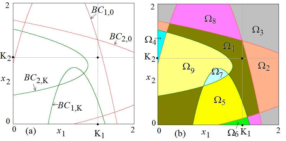
Figure 1: Parameters: $\gamma_{1}=\gamma_{2}=1$, $\tau_{1}=\tau_{2}=4$, $N_{1}=N_{2}=1.5,$ as in all the figures of the paper. $K_{1}=1.4$ and $K_{2}=1.1$. The gray lines mark the border of the phase plane $D=\left[0,K_{1}\right]\times\left[0,K_{2}\right]$. A black dot marks the intersection of these two lines. In (a) the border curves $BC_{1,0}$ and $BC_{2,0}$ in red, the border curves $BC_{1,K}$ and $BC_{2,K}$ in green. In (b) the regions $\Omega_{j}$ of the phase plane are evidenced by different colors. To better clarify the shape of the constraints, we illustrate all the figures in the phase plane $[0,2]\times\left[0,2\right],$ although the region of interest of the model is $D\subset\left[0,N_{1}\right]\times\left[0,N_{2}\right]$.

The positive quadrant of the phase plane is thus partitioned in nine regions, in each of which a different definition (i.e. a different function) is to be applied. Let us define the regions as follows:

$$\begin{array}[c]{lll}\Omega_{1}&=&\left\{\left(x_{1},x_{2}\right)|0\leq F_{1}\left(x_{1},x_{2}\right)\leq K_{1}\text{ and }0\leq F_{2}\left(x_{1},x_{2}\right)\leq K_{2}\right\}\\ \Omega_{2}&=&\left\{\left(x_{1},x_{2}\right)|F_{1}\left(x_{1},x_{2}\right)\leq 0\text{ and }0\leq F_{2}\left(x_{1},x_{2}\right)\leq K_{2}\right\}\\ \Omega_{3}&=&\left\{\left(x_{1},x_{2}\right)|F_{1}\left(x_{1},x_{2}\right)\leq 0\text{ and }F_{2}\left(x_{1},x_{2}\right)\leq 0\right\}\\ \Omega_{4}&=&\left\{\left(x_{1},x_{2}\right)|F_{1}\left(x_{1},x_{2}\right)\leq 0\text{ and }F_{2}\left(x_{1},x_{2}\right)\geq K_{2}\right\}\\ \Omega_{5}&=&\left\{\left(x_{1},x_{2}\right)|F_{1}\left(x_{1},x_{2}\right)\geq K_{1}\text{ and }0\leq F_{2}\left(x_{1},x_{2}\right)\leq K_{2}\right\}\\ \Omega_{6}&=&\left\{\left(x_{1},x_{2}\right)|F_{1}\left(x_{1},x_{2}\right)\geq K_{1}\text{ and }F_{2}\left(x_{1},x_{2}\right)\leq 0\right\}\\ \Omega_{7}&=&\left\{\left(x_{1},x_{2}\right)|F_{1}\left(x_{1},x_{2}\right)\geq K_{1}\text{ and }F_{2}\left(x_{1},x_{2}\right)\geq K_{2}\right\}\\ \Omega_{8}&=&\left\{\left(x_{1},x_{2}\right)|0\leq F_{1}\left(x_{1},x_{2}\right)\leq K_{1}\text{ and }F_{2}\left(x_{1},x_{2}\right)\leq 0\right\}\\ \Omega_{9}&=&\left\{\left(x_{1},x_{2}\right)|0\leq F_{1}\left(x_{1},x_{2}\right)\leq K_{1}\text{ and }F_{2}\left(x_{1},x_{2}\right)\geq K_{2}\right\}\end{array}$$ (9)

so that the map in each region is given by:

$$\begin{array}[c]{ll}\left(x_{1},x_{2}\right)\in\Omega_{1}&:(x_{1}^{\prime},x_{2}^{\prime})=(F_{1}\left(x_{1},x_{2}\right),F_{2}\left(x_{1},x_{2}\right))\\ \left(x_{1},x_{2}\right)\in\Omega_{2}&:(x_{1}^{\prime},x_{2}^{\prime})=(0,F_{2}\left(x_{1},x_{2}\right))\\ \left(x_{1},x_{2}\right)\in\Omega_{3}&:(x_{1}^{\prime},x_{2}^{\prime})=(0,0)\\ \left(x_{1},x_{2}\right)\in\Omega_{4}&:(x_{1}^{\prime},x_{2}^{\prime})=(0,K_{2})\\ \left(x_{1},x_{2}\right)\in\Omega_{5}&:(x_{1}^{\prime},x_{2}^{\prime})=(K_{1},F_{2}\left(x_{1},x_{2}\right))\\ \left(x_{1},x_{2}\right)\in\Omega_{6}&:(x_{1}^{\prime},x_{2}^{\prime})=(K_{1},0)\\ \left(x_{1},x_{2}\right)\in\Omega_{7}&:(x_{1}^{\prime},x_{2}^{\prime})=(K_{1},K_{2})\\ \left(x_{1},x_{2}\right)\in\Omega_{8}&:(x_{1}^{\prime},x_{2}^{\prime})=(F_{1}\left(x_{1},x_{2}\right),0)\\ \left(x_{1},x_{2}\right)\in\Omega_{9}&:(x_{1}^{\prime},x_{2}^{\prime})=(F_{1}\left(x_{1},x_{2}\right),K_{2})\end{array}$$ (10)

We notice that the points on the boundaries of the regions may belong to two different regions: as the map is continuous, it does not matter whether a point is considered belonging to one region or to the other, as the evaluated value of the map is the same. From the definition it follows immediately that the rectangle

$$D=\left[0,K_{1}\right]\times\left[0,K_{2}\right]$$ (11)

is absorbing, as any point of the plane is mapped in $D$ in one iteration and an orbit cannot escape from it, thus $D$ is our region of interest. In general, depending on the values of the parameters, only a few of the regions $\Omega_{j}$ for $j=1,...,9$ may have a portion, or subregion, present in $D$, say $\Omega_{j}\cap D\neq\varnothing,$ as shown for example in Fig. 1b. In any case, the behavior of the map in the other regions, not entering $D,$ may be easily explained. To this purpose, let us introduce first a few remarks on the fixed points that the system can have.

The fixed points of the system, satisfying $T(x_{1},x_{2})=(x_{1},x_{2})$, are associated with the solutions of several equations. For sure we have some fixed points on the axes, which correspond to disappearance (i.e. extinction) of one population. From $F_{i}\left(0,0\right)=\left(0,0\right)$ for $i=1,2$ we have that the origin $(0,0)$ is always a fixed point. Although, as we shall see, it is locally unstable, all the points belonging to region $\Omega_{3}$ are mapped into the origin in one iteration (and then they are fixed).

The axes are invariant, as considering a point $(x_{1},0)$ on the $x_{1}$ axis we have that $T(x_{1},0)=(T_{1}(x_{1},0),T_{2}(x_{1},0))=(T_{1}(x_{1},0),0)$ still belongs to the axis, and

$$T_{1}(x_{1},0)=\left\{\begin{array}[c]{ccc}0&\text{if}&F_{1}\left(x_{1},0\right)\leq 0\\ F_{1}\left(x_{1},0\right)&\text{if}&0\leq F_{1}\left(x_{1},0\right)\leq K_{1}\\ K_{1}&\text{if}&F_{1}\left(x_{1},0\right)\geq K_{1}\end{array}\right.$$ (12)

where

$$F_{1}\left(x_{1},0\right)=x_{1}\left[1+\gamma_{1}x_{1}\tau_{1}\left(1-\frac{x_{1}}{N_{1}}\right)\right].$$ (13)

Thus, region $\Omega_{6}$, whose points are all mapped in $(K_{1},0)$ in one iteration, necessarily has non-empty intersection with the rectangle $D,$ and $(K_{1},0)$ is a fixed point of the map. Moreover, considering the restriction $t_{1}(x_{1})\equiv T_{1}\left(x_{1},0\right)$ we have that $t_{1}(x_{1})=x_{1}$ is satisfied for $x_{1}^{\ast}=0$ which is a fixed point (representing the origin), and $x_{1}=N_{1}$ which is virtual for $K_{1}<N_{1}$ (constraint that we consider in the model). Thus the map $x_{1}(t+1)=t_{1}(x_{1}(t))$ has a fixed point $x_{1}^{\ast}=K_{1}$ where the piecewise smooth function $t_{1}(x_{1})$ has a flat branch, which means that the fixed point $(K_{1},0)$ always exists and is superstable (for the restriction). While considering $\frac{d}{dx_{1}}t_{1}(x_{1})=1+2\gamma_{1}\tau_{1}x_{1}-3\frac{\gamma_{1}\tau_{1}}{N_{1}}x_{1}^{2}$ we have $\frac{d}{dx_{1}}t_{1}(0)=1$ and $\frac{d^{2}}{d^{2}x_{1}}t_{1}(x_{1})=2\gamma_{1}\tau_{1}-6\frac{\gamma_{1}\tau_{1}}{N_{1}}x_{1}$ leads to $\frac{d^{2}}{d^{2}x_{1}}t_{1}(0)=2\gamma_{1}\tau_{1}>0$ so that the fixed point $x_{1}^{\ast}=0$ is repelling on its right side, that is, the origin $(0,0)$ is repelling along the $x_{1}$ direction.

Similarly for the second axis, we have that $T(0,x_{2})=(T_{1}(0,x_{2}),T_{2}(0,x_{2}))=(0,T_{2}(0,x_{2}))$ with

$$T_{2}(0,x_{2})=\left\{\begin{array}[c]{ccc}0&\text{if}&F_{2}\left(0,x_{2}\right)\leq 0\\ F_{2}\left(0,x_{2}\right)&\text{if}&0\leq F_{2}\left(0,x_{2}\right)\leq K_{2}\\ K_{2}&\text{if}&F_{2}\left(0,x_{2}\right)\geq K_{2}\end{array}\right.$$ (14)

where

$$F_{2}\left(0,x_{2}\right)=x_{2}\left[1+\gamma_{2}x_{2}\tau_{2}\left(1-\frac{x_{2}}{N_{2}}\right)\right].$$ (15)

So region $\Omega_{4}$ (whose points are all mapped in $(0,K_{2})$ in one iteration) intersects the rectangle $D$ and $(0,K_{2})$ is a superstable fixed point of the restriction, while the origin $(0,0)$ is repelling along the $x_{2}$ direction. The proof is the same as the one given above for the $x_{1}$ axis, changing the index $i=1$ into $i=2$. Regarding our example, the one-dimensional map $x_{2}(t+1)=t_{2}(x_{2}(t))\equiv T_{2}(0,x_{2}(t))$ is shown in Fig. 2a.

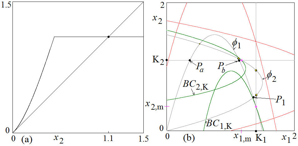
Figure 2: Parameters as in Fig. 1. In (a) function $t_{2}\left(x_{2}\right)$ for $x_{2}\in\left[0,N_{2}\right]$, the black dot is a superstable equilibrium. In (b) the reaction curves $\phi_{1}$ and $\phi_{2},$ as well as the lines $x_{1}=K_{1}$ and $x_{2}=K_{2},$ are in gray. Black dots are feasible equilibria, black dots with yellow interior are virtual equilibria. The dots in pink are the points $(x_{1,m},K_{2})$ and $(K_{1},x_{2,m}).$

Below we shall complete the comments regarding the fixed points $(K_{1},0)$ and $(0,K_{2})$ on the axes for the two-dimensional map $T$.

Other fixed points $(x_{1}^{\ast},x_{2}^{\ast})$ may exist as solutions of the equations

$$\left\{\begin{array}[c]{c}x_{1}R_{1}(x_{1})=x_{2}\\ x_{2}R_{2}(x_{2})=x_{1}\end{array}\right.$$

when belonging to region $\Omega_{1}$ (otherwise they are so-called virtual fixed points). These fixed points can be seen in the phase plane as intersection points of the two reaction curves

$$\phi_{1}:\ x_{2}=x_{1}R_{1}(x_{1})\text{ and }\phi_{2}:x_{1}=x_{2}R_{2}(x_{2}),$$ (16)

and the number of such points can be at most four.

Moreover, also fixed points $(K_{1},x_{2}^{\ast})$ may exist, associated with the solutions of the equation $x_{2}R_{2}(x_{2})=K_{1},$ when belonging to region $\Omega_{5}\cap D.$ Also these fixed points can be graphically seen in the phase plane as intersection points of the two curves $x_{1}=K_{1}$ (vertical straight line) and $\phi_{2}$. Similarly, fixed points of type $(x_{1}^{\ast},K_{2})$ associated with the solutions of the equation $x_{1}R_{1}(x_{1})=K_{2}$ (intersection points of the horizontal straight line $x_{2}=K_{2}$ and $\phi_{1}$) may exist, when belonging to region $\Omega_{9}\cap D.$

The fixed points of the example shown in Fig. 1 are evidenced in Fig. 2b where the two curves$\ \phi_{1}$ and $\phi_{2}$ (having a unimodal shape) are drawn, together with the straight lines $x_{1}=K_{1}$ and $x_{2}=K_{2}.$ Besides in the origin, the curves$\ \phi_{1}$ and $\phi_{2}$ have three intersection points, but two of them belong to region $\Omega_{9}$ and are outside $D$, while the third one, say $P_{1},$ belongs to region $\Omega_{1}$ in $D$ and thus it is a true fixed point of the map. On the vertical line $x_{1}=K_{1}$ a fixed point is $(K_{1},0)$ on the axis and, as we shall see, it is superstable. Then two more solutions of $x_{2}R_{2}(x_{2})=K_{1}$ exist, but both points belong to region $\Omega_{1}$ and thus are virtual fixed points. Differently, on the horizontal line $x_{2}=K_{2},$ besides the superstable fixed point $(0,K_{2})$ on the vertical axis, there are two more fixed points of the map, $P_{a}=(x_{1,a}^{\ast},K_{2})$ and $P_{b}=(x_{1,b}^{\ast},K_{2}),$ as both belong to region $\Omega_{9}\cap D.$ We shall return on these fixed points below.

The definitions of the map in the several regions $\Omega_{j}$ lead to different kinds of degeneracy. For example, when a portion of region $\Omega_{7}$ exists in $D$, then all the points of that region are mapped into a unique point: the corner $(K_{1},K_{2})$ of the absorbing rectangle $D,$ which means that in region $\Omega_{7}$ we have two degeneracies, that is, two eigenvalues equal to zero in the Jacobian matrix at any point of $\Omega_{7}$.

Thus, one more fixed point may be given by the point $P=(K_{1},K_{2})$ when it belongs to $\Omega_{7}\cap D$ (and in such a case this fixed point is superstable: both eigenvalues are equal to zero). While when $(K_{1},K_{2})$ does not belong to $\Omega_{7}\cap D,$ then for the dynamics of the points in region $\Omega_{7}$ it is enough to consider the trajectory of only one point: $(K_{1},K_{2})$.

Other regions with double degeneracies are $\Omega_{3},$ $\Omega_{4}$ and $\Omega_{6}$ as all of them are mapped into fixed points, $(0,0),$ $(0,K_{2})$ and $(K_{1},0),$ respectively. These fixed points do not deserve for other comments apart from their local stability/instability: as we have seen, the origin is unstable while we shall see below (in Property 2) that the two other fixed points on the axes are superstable when $\Omega_{4}$ and $\Omega_{6}$ intersect $D$ in a set of positive measure, stable otherwise.

There are other degeneracies which are immediate from the definition of the map, due to the regions bounded by the border curves $BC_{i,K}$ (see Fig. 1a). Considering the portion of the phase plane which is bounded by the border curve $BC_{1,K},$ we have that the whole region is mapped onto the line $x_{1}=K_{1}.$ Similarly the whole region bounded by the border curve $BC_{2,K}$ is mapped onto the line $x_{2}=K_{2}.$ Thus, in both regions we have one degeneracy as the Jacobian matrix in all the points of these regions has one eigenvalue equal to zero. As a whole region is mapped into a segment of straight line, the dynamics can be associated with the points of those particular segments. In particular, the stability/instability of the fixed points belonging to these lines can be investigated considering the restriction of the map to these lines, when they belong to the proper region (that is, when they are real fixed points of $T$ and not virtual). Let us first notice the following

Property 1

The three curves $x_{2}=K_{2}$, $BC_{2,K}$ and $\phi_{2}$ all intersect in the point $\left(x_{1,m},K_{2}\right)$, where $x_{1,m}=K_{2}\tau_{2}\left(1-\frac{K_{2}}{N_{2}}\right)$. The three curves $x_{1}=K_{1}$, $BC_{1,K}$ and $\phi_{1}$ all intersect in the point $\left(K_{1},x_{2,m}\right)$, where $x_{2,m}=K_{1}\tau_{1}\left(1-\frac{K_{1}}{N_{1}}\right)$.

Proof. In fact, $x_{2}=K_{2}$ intersects $BC_{2,K}:x_{1}=\left[1+\gamma_{2}x_{2}R_{2}\left(x_{2}\right)-\frac{K_{2}}{x_{2}}\right]/\gamma_{2}$ in the point $x_{1,m}=K_{2}R_{2}(K_{2})=K_{2}\tau_{2}\left(1-\frac{K_{2}}{N_{2}}\right),$ and also $x_{2}=K_{2}$ intersects $\phi_{2}:x_{1}=x_{2}R_{2}(x_{2})=x_{2}\tau_{2}\left(1-\frac{x_{2}}{N_{2}}\right)$ in the same point, as it is immediately evident. Similarly for the other curves (these points are evidenced in Fig. 2b).   

So, let us consider $x_{2}=K_{2}$ and the segment of this line for $x_{1}\geq 0$ and $x_{1}\leq x_{1,m},$ where $x_{1,m}$ is defined in Property 1. Then the restriction of the map to this segment is invariant, and on it the dynamics are given (for $0\leq x_{1}\leq x_{1,m}$) by the one-dimensional map

$$x_{1}(t+1)=f_{1}\left(x_{1}(t)\right)\ ,\ \ f_{1}\left(x_{1}\right)=\left\{\begin{array}[c]{ccc}0&\text{if}&F_{1}\left(x_{1},K_{2}\right)\leq 0\\ F_{1}\left(x_{1},K_{2}\right)&\text{if}&0\leq F_{1}\left(x_{1},K_{2}\right)\leq K_{1}\\ K_{1}&\text{if}&F_{1}\left(x_{1},K_{2}\right)\geq K_{1}\end{array}\right.$$ (17)

where

$$F_{1}\left(x_{1},K_{2}\right)=x_{1}\left[1-\gamma_{1}K_{2}+\gamma_{1}x_{1}\tau_{1}\left(1-\frac{x_{1}}{N_{1}}\right)\right]$$ (18)

The point $x_{1}=0$ corresponds to the fixed point $(0,K_{2})$ of $T$, and fixed points with positive values internal to the range $[0,K_{1}]$ are thus associated with the solutions of a quadratic equation, leading to

$$x_{1,b,a}^{\ast}=\frac{N_{1}}{2}\pm\sqrt{\left(\frac{N_{1}}{2}\right)^{2}-\frac{K_{2}N_{1}}{\tau_{1}}}$$

moreover

$$\frac{d}{dx_{1}}F_{1}\left(x_{1},K_{2}\right)=1-\gamma_{1}K_{2}+x_{1}\gamma_{1}\tau_{1}\left(2-\frac{3x_{1}}{N_{1}}\right)$$ (19)

so that $\frac{d}{dx_{1}}F_{1}\left(0,K_{2}\right)=1-\gamma_{1}K_{2}<1$, which implies that this fixed point is attracting also on the direction of the line (as the derivative is either zero, when the constraint is active, or positive and smaller that 1), and

$$\frac{d}{dx_{1}}F_{1}\left(x_{1,b,a}^{\ast},K_{2}\right) =1+2\gamma_{1}K_{2}-x_{1,b,a}^{\ast}\gamma_{1}\tau_{1}$$

$$=1+2\gamma_{1}K_{2}-\gamma_{1}\tau_{1}\left(\frac{N_{1}}{2}\pm\sqrt{\left(\frac{N_{1}}{2}\right)^{2}-\frac{K_{2}N_{1}}{\tau_{1}}}\right)$$

Summarizing, these two more are fixed points of the two-dimensional map only if $x_{1,a}^{\ast}\leq x_{1,m}$ and $x_{1,b}^{\ast}\leq x_{1,m}$ (as it occurs in the example shown in Fig. 2b), and their stability depends on the value of $\frac{d}{dx_{1}}f_{1}\left(x_{1,b,a}\right)$. When $|\frac{d}{dx_{1}}f_{1}\left(x_{1,b,a}\right)|<1$ (resp. $>1$) the fixed points are attracting (resp. repelling). In the example considered in Fig. 2b both fixed points $P_{a}=(x_{1,a}^{\ast},K_{2})$ and $P_{b}=(x_{1,b}^{\ast},K_{2})$ are repelling.

We can reason similarly for the restriction of the map on the straight line $x_{1}=K_{1},$ for $0\leq x_{2}\leq x_{2,m},$ where $x_{2,m}$ is defined in Property 1, which is given by the one-dimensional map

$$x_{2}(t+1)=f_{2}\left(x_{2}(t)\right)\ ,\ \ f_{2}\left(x_{2}\right)=\left\{\begin{array}[c]{ccc}0&\text{if}&F_{2}\left(K_{1},x_{2}\right)\leq 0\\ F_{2}\left(K_{1},x_{2}\right)&\text{if}&0\leq F_{2}\left(K_{1},x_{2}\right)\leq K_{2}\\ K_{2}&\text{if}&F_{2}\left(K_{1},x_{2}\right)\geq K_{2}\end{array}\right.$$ (20)

where

$$F_{2}\left(K_{1},x_{2}\right)=x_{2}\left[1-\gamma_{2}K_{1}+\gamma_{2}x_{2}\tau_{2}\left(1-\frac{x_{2}}{N_{2}}\right)\right]$$ (21)

Thus, besides $x_{2}=0,$ which represents the fixed point ($K_{1},0$), the fixed points are associated with the solutions of a quadratic equation, leading to

$$x_{2,b,a}^{\ast}=\frac{N_{2}}{2}\pm\sqrt{\left(\frac{N_{2}}{2}\right)^{2}-\frac{K_{1}N_{2}}{\tau_{2}}}$$

moreover

$$\frac{d}{dx_{2}}F_{2}\left(K_{1},x_{2}\right)=1-\gamma_{2}K_{1}+x_{2}\gamma_{2}\tau_{2}\left(2-\frac{3x_{2}}{N_{2}}\right)$$ (22)

so that $\frac{d}{dx_{2}}F_{2}\left(K_{1},0\right)=1-\gamma_{2}K_{1}<1$, which implies that this fixed point is attracting also on the direction of the line, and

$$\frac{d}{dx_{2}}F_{2}(K_{1},x_{2,b,a}^{\ast}) =1+2\gamma_{2}K_{1}-x_{2,b,a}^{\ast}\gamma_{2}\tau_{2}$$

$$=1+2\gamma_{2}K_{1}-\gamma_{2}\tau_{2}\left(\frac{N_{2}}{2}\pm\sqrt{\left(\frac{N_{2}}{2}\right)^{2}-\frac{K_{1}N_{2}}{\tau_{2}}}\right)$$

These solutions are fixed points of the two-dimensional map only if $x_{2,a}^{\ast}\leq x_{2,m}$ and $x_{2,b}^{\ast}\leq x_{2,m}.$

With the parameter values used in the example shown in Fig. 2b both the inequalities given above are not satisfied and these points are called virtual fixed points (i.e. they are not fixed points of the two-dimensional map).

We can also end the comments on the fixed points on the axes for the two-dimensional map $T$. In fact, let us consider $\left(0,K_{2}\right).$ We have already seen that along the axes $x_{1}=0$ there is a zero eigenvalue, and now we can complete with the eigenvalue along the invariant segment on $x_{2}=K_{2}.$ From the definition of the restriction in (17) and (18) we have that either this point (the origin of the restriction) is superstable (which occurs when $\Omega_{4}$ intersects $D$ in a set of positive measure), or stable, as we have $0<\frac{d}{dx_{1}}F_{1}\left(0,K_{2}\right)<1.$ Similarly we can reason for the other fixed point $(K_{1},0).$

This leads to an important property of the model: the two single ”segregation states” always exist and attract some points of the phase plane. How many points depends on the structure of the basins of attraction of these fixed points, and on the existence or not of other attracting sets having states with positive values (not converging to the axes). However, some results are already known from the remarks written above: as all the points of the region $\Omega_{2}$ are mapped into the $x_{2}$ axis, which is trapping and on which we know there is convergence to the fixed point $(0,K_{2})$, so we can immediately conclude that all the points of region $\Omega_{2}$ belong to the basin of attraction of $(0,K_{2}).$ Similarly, all the points of region $\Omega_{8}$ belong to the basin of attraction of the fixed point $(K_{1},0).$ We shall see some examples below. We can so state the following

Property 2

Two stable fixed points always exist in map $T$ given in (3): $\left(0,K_{2}\right)$ and $\left(K_{1},0\right)$. The points of region $\Omega_{4}$ are mapped into $\left(0,K_{2}\right)$ and those of region $\Omega_{2}$ converge to $\left(0,K_{2}\right)$. If $\Omega_{4}\cap D$ has positive measure, then $\left(0,K_{2}\right)$ is superstable for the two-dimensional map $T$. The points of region $\Omega_{6}$ are mapped into $\left(K_{1},0\right)$, and those of region $\Omega_{8}$ converge to $\left(K_{1},0\right)$. If $\Omega_{6}\cap D$ has positive measure, then $\left(K_{1},0\right)$ is superstable for the two-dimensional map $T$.

In the example considered in Fig.s 1,2 the two fixed points $(K_{1},0)$ and $(0,K_{2})$ on the axes are superstable for map $T$. Besides them, map $T$ has two more fixed points $P_{a}=(x_{1,a}^{\ast},K_{2})$ and $P_{b}=(x_{1,b}^{\ast},K_{2})$ in region $\Omega_{9}\cap D$ which are unstable, and one more fixed point: $P_{1}\in\phi_{1}\cap\phi_{2}$ belonging to region $\Omega_{1}\cap D.$ At $P_{1}$ the map has a smooth definition $(x_{1}(t+1),x_{2}(t+1))=(F_{1}(x_{1}(t),x_{2}(t)),F_{2}(x_{1}(t),x_{2}(t)))$, and the stability of this fixed point depends on the eigenvalues of the Jacobian matrix evaluated at $P_{1}.$ In our example also this fixed point $P_{1}$ is unstable. $P_{1}$ and $P_{a}$ belong to the frontiers separating the basins of attraction. A third (chaotic) attractor exists, as shown in Fig. 3a.

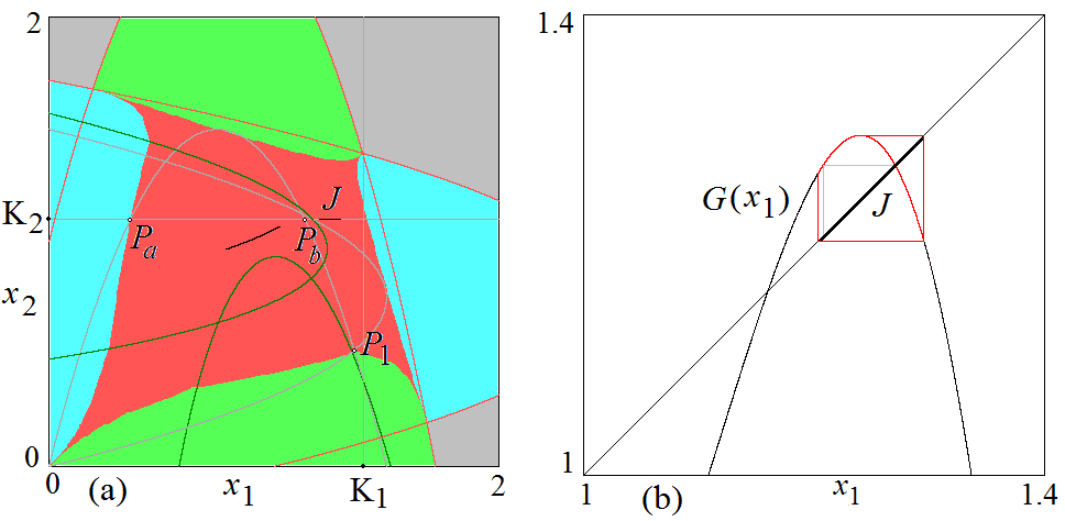
Figure 3: Parameters as in Fig. 1. In (a) basin of attraction of $\left(0,K_{1}\right)$ in green, basin of attraction of $\left(0,K_{2}\right)$ in azure, basin of attraction of $\left(0,0\right)$ in gray and basin of attraction of the chaotic attractor in red. $P_{a}$, $P_{b}$ and $P_{1}$ are unstable equilibria. In (b) first return map $G\left(x_{1}\right)$ on $x_{2}=K_{2}$. $J$ represents an invariant segment, it is the portion of the chaotic attractor of map $T$ that lies on $x_{2}=K_{2}$. The gray lines show that the fixed point of the first return map is homoclinic.

A trajectory on this attracting set consist of points which alternate from region $\Omega_{9}$ to region $\Omega_{1}.$ This may be of great help as the dynamics of $T$ can thus be investigated by use of a one dimensional map: the first return map on a segment of the straight line $x_{2}=K_{2}$. In fact, the points of the attracting set belonging to region $\Omega_{9}$ are mapped on the line $x_{2}=K_{2}$ above the point $x_{1,m}=K_{2}\tau_{2}\left(1-\frac{K_{2}}{N_{2}}\right)$ (in region $\Omega_{1}).$ Thus, a point $(x_{1},K_{2})$ of the attractor is mapped in $T(x_{1},K_{2})=(F_{1}\left(x_{1},K_{2}\right),F_{2}\left(x_{1},K_{2}\right))\in\Omega_{9}$ and then a second iteration leads to $T^{2}(x_{1},K_{2})=(F_{1}(F_{1}\left(x_{1},K_{2}\right),F_{2}\left(x_{1},K_{2}\right)),K_{2})=:(G\left(x_{1}\right),K_{2})\in\Omega_{1}.$ So it can be investigated by use of the following one-dimensional first return map on $x_{2}=K_{2}$:

$$x_{1}(t+1)=G\left(x_{1}(t)\right)$$ (23)

$$G\left(x_{1}\right)=F_{1}\left(x_{1}\left(1-\gamma_{1}K_{2}+\gamma_{1}x_{1}\tau_{1}\left(1-\frac{x_{1}}{N_{1}}\right)\right),K_{2}\left(1-\gamma_{2}x_{1}+\gamma_{2}K_{2}\tau_{2}\left(1-\frac{K_{2}}{N_{2}}\right)\right)\right)$$ (24)

in the range $x_{1,m}=K_{2}\tau_{2}\left(1-\frac{K_{2}}{N_{2}}\right)<x_{1}<K_{1}.$ This one-dimensional map, in our example, is shown in Fig. 3b, evidencing the invariant interval $J$ on which the dynamics seem to be chaotic. Indeed, the fixed point in Fig. 3b inside the invariant segment $J,$ which corresponds to an unstable 2-cycle of $T$, is homoclinic. This invariant segment $J$ corresponds to the segment of the attractor on the straight line $x_{2}=K_{2}$ in Fig. 3a.

As already remarked in the Introduction, the goal of this paper is to investigate the role of the constraints, which are the values of $K_{1}$ and $K_{2}.$ In doing so, here we investigate this only in the case in which the two states (groups or populations) represented by $x_{1}$ and $x_{2}$ are in some way symmetric, as characterized by parameters having the same values. Thus, in the next section we shall consider the parameters $N\equiv N_{1}=N_{2}$, $\tau\equiv\tau_{1}=\tau_{2}$ and $\gamma\equiv\gamma_{1}=\gamma_{2}$. Nevertheless, in piecewise smooth dynamical systems as the present one, the other parameters may also be relevant. This aspect and in particular the investigation of the role of the constraints in the generic case, with different parameter values for the two populations, is left for further studies.

Here we are mainly interested in the role played by the two constraints $K_{1}$ and $K_{2}$ which represent possible regulatory policy choices. Recall that $K_{1}$ and $K_{2}$ represent the upper limit number of individuals of a given group allowed to enter the system. We shall see a two-dimensional bifurcation diagrams which immediately emphasizes the attracting cycles existing as a function of the parameters $(K_{1},K_{2}).$ In the next section we shall describe several regions in that parameter plane which lead to interesting dynamic behaviors.

3 Border Collision Bifurcations and global analysis of the dynamics

Let us first consider the relevant dynamics occurring as a function of $(K_{1},K_{2})$, let us call them ”the control parameters”, when the other parameters are fixed (in our representative case at the values considered in the figures of the previous section: $N=1.5$, $\tau=4$ and $\gamma=1$). As in this paper we restrict our analysis to populations with the same characteristics (in the parameters $\gamma_{i},$ $\tau_{i}$ and $N_{i}),$ the bifurcations occurring in the parameters $(K_{1},K_{2})$ are obviously symmetric, which leads to the following Property:

Property 3 (Symmetric parameter plane)

Let $N\equiv N_{1}=N_{2}$, $\tau\equiv\tau_{1}=\tau_{2}$ and $\gamma\equiv\gamma_{1}=\gamma_{2}$. Let the control parameters have the values $\left(K_{1},K_{2}\right)=\left(\xi,\eta\right)$ and let $\left\{\left(a\left(t\right),b\left(t\right)\right),\;t>0\right\}$ be the trajectory associated with the initial condition $\left(a\left(0\right),b\left(0\right)\right)$. Then $\left\{\left(b\left(t\right),a\left(t\right)\right),\;t>0\right\}$ is the trajectory associated with the initial condition $\left(b\left(0\right),a\left(0\right)\right)$ when the control parameters have the values $\left(K_{1},K_{2}\right)=\left(\eta,\xi\right)$.

That is, via a change of variable $x_{2}:=x_{1}$ and $x_{1}:=x_{2}$ we have the same dynamics when $K_{1}$ and $K_{2}$ are exchanged. This explains the symmetric structure with respect to the main diagonal in the two-dimensional bifurcation diagram shown in Fig. 4.

As a particular case of Property 3 we have another property when $K_{1}=K_{2}$ (on the diagonal of the two-dimensional bifurcation diagram of Fig. 4):

Property 4 (Symmetric phase plane)

Let $N\equiv N_{1}=N_{2}$, $\tau\equiv\tau_{1}=\tau_{2}$, $\gamma\equiv\gamma_{1}=\gamma_{2}$ and $K\equiv K_{1}=K_{2}$. Then:

1. Let $(a(t),b(t))$ for any integer $t>0$ be the trajectory associated with the initial condition $\left(a\left(0\right),b\left(0\right)\right)$, then $\left(b\left(t\right),a\left(t\right)\right)$ for any integer $t>0$ is the trajectory associated with the initial condition $\left(b\left(0\right),a\left(0\right)\right).$

2. On the diagonal $\Delta$ of the phase plane map $T$ reduces to a one-dimensional system. From initial conditions $x_{1}\left(0\right)=x_{2}\left(0\right)$ it will be $x_{1}\left(t\right)=x_{2}\left(t\right)$ for any integer $t>0$ and the iterates are given by the one-dimensional map defined as $x\left(t+1\right)=T_{\Delta}\left(x\left(t\right)\right)$ with

   $$T_{\Delta}(x)=\left\{\begin{array}[c]{ccc}0&if&F_{\Delta}\left(x\right)\leq 0\\ F_{\Delta}\left(x\right)&\text{if}&0\leq F_{\Delta}\left(x\right)\leq K\\ K&if&F_{\Delta}\left(x\right)\geq K\end{array}\right.$$ (25)

   where $x\equiv x_{1}=x_{2}$ and $F_{\Delta}\left(x\right)\equiv F_{1}\left(x,x\right)=F_{2}\left(x,x\right)$ is given by

   $$F_{\Delta}\left(x\right)=x\left[1-\gamma x+\gamma x\tau\left(1-\frac{x}{N}\right)\right].$$ (26)

Clearly for the points of the phase plane outside the diagonal $x_{1}=x_{2}$ the Property (4i) stated above holds. Moreover, it is worth noting that Property (4i) implies that an invariant set of the two-dimensional map is either symmetric with respect to the diagonal $\Delta$ $(x_{1}=x_{2})$ of the phase plane, or the symmetric invariant set of it also exists.

As an example let us show the possible bifurcations occurring in the parameter plane of the control parameters $(K_{1},K_{2})$ in the range $\left[0,N_{1}\right]\times\left[0,N_{2}\right]$ as reported in Fig. 4. As the model is symmetric (Property (4i)), we can just analyze the dynamics of the model for $K_{2}\geq K_{1}$, i.e. taking into consideration only the region above the diagonal in the two-dimensional bifurcation diagram of Fig. 4, as the dynamics and bifurcations for parameters on the symmetric side, i.e. for $K_{2}\leq K_{1}$, are of the same kind (by Property 3).

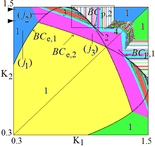
Figure 4: Two dimensional bifurcation diagram in the $\left(K_{1},K_{2}\right)$-parameter plane for the map $T$. Different colors are related to attracting cycles of different periods $n\leq 30$, the white region corresponds either to chaotic attractors or to cycles of higher periodicity.

In Fig. 4 we highlights some BCB curves, which we shall explain below.

It is worth to note that as the parameters $K_{1}$ and $K_{2}$ influence the borders of the regions at which the piecewise smooth map changes its definition, all the bifurcations that we observe in Fig. 4 are expected to be border collision bifurcations. Indeed, even if this is not a sufficient condition to state that all the curves are related to BCBs, the high degeneracy of the map leads to this particular result.

3.1 Case $K_{1}=K_{2}$

Let us first describe the dynamics occurring in the phase plane when the parameters belong to the diagonal $K_{1}=K_{2}$ of the two-dimensional bifurcation diagram, and let $K\equiv K_{1}=K_{2}.$ As already shown above, for points in the phase plane belonging to the diagonal where $x\equiv x_{1}=x_{2}$ we can consider the one-dimensional piecewise smooth continuous map $x(t+1)=T_{\Delta}(x(t))$ (given in (25) and (26)).

The map $T_{\Delta}$ has fixed points satisfying the equation $F_{\Delta}(x)=x$, leading to a fixed point in $x=0$ (representing the origin) and $x^{\ast}=N(1-\frac{1}{\tau})$ which exists (positive) only for $\tau>1.$ It is a real fixed point if $N(1-\frac{1}{\tau})\leq K,$ otherwise $x^{\ast}=K$ is a fixed point on the flat branch of the function. We can state the following

Property 5

Let $N\equiv N_{1}=N_{2}$, $\tau\equiv\tau_{1}=\tau_{2}>1$, $\gamma\equiv\gamma_{1}=\gamma_{2}$ and $K\equiv K_{1}=K_{2}$.

1. For $K<N\left(1-\frac{1}{\tau}\right)$ map $T_{\Delta}$ has a positive fixed point $x^{\ast}=K$ belonging to a flat branch, while for $K>N\left(1-\frac{1}{\tau}\right)$ map $T_{\Delta}$ has a positive fixed point $x^{\ast}=N(1-\frac{1}{\tau})$ belonging to a smooth branch. At $K=N\left(1-\frac{1}{\tau}\right)$ a border collision of the fixed point $x^{\ast}$ occurs. If the bifurcation value satisfies $K<\overline{K}$ (resp. $K>\overline{K}$), where

   $$\overline{K}=\frac{2\gamma(\tau-1)N+\sqrt{(2\gamma(\tau-1)N)^{2}+24N\gamma\tau}}{6\gamma\tau}$$ (27)

   then increasing $K$ the result of the border collision is persistence of a stable fixed point (resp. a repelling fixed point and a superstable 2-cycle with periodic points $\left\{K,\;T_{\Delta}\left(K\right)\right\}$).

2. For $K>T_{\Delta}\left(x_{c}\right)$ where

   $$x_{c}=\frac{(\tau-1)N}{3\tau}+\sqrt{\left(\frac{(1-\tau)N}{3\tau}\right)^{2}+\frac{N}{3\gamma\tau}}$$ (28)

   map $T_{\Delta}$ is smooth. At $K=T_{\Delta}(x_{c}$) there is a transition from piecewise-smooth to smooth.

Proof. We notice that at $K=N(1-\frac{1}{\tau})$ for the two-dimensional map $T$ the fixed point undergoes a codimension-two border collision as two borders are crossed simultaneously $(\phi_{1}$ and $\phi_{2})$.

At the bifurcation value $K=N(1-\frac{1}{\tau})$ the fixed point $x^{\ast}$ merges with the border point (point in which the map changes its definition), so it is a border collision. Increasing the value of $K$, the fixed point $x^{\ast}$ moves from the flat branch to the smooth branch. The result of this collision is completely predictable, as already remarked in the literature (see for example [25] and references therein). In fact, in the one-dimensional case the skew-tent map can be used as a border collision normal form, which means that in general, apart from codimension-two bifurcation cases, the slopes of the two functions on the right and left side of the border point at the BCB parameters values determine which kind of dynamic behavior will appear after the BCB. In our case we have that the slope on the left side of the border point is zero while on the right side it is given by $F_{\Delta}^{\prime}\left(K\right)$ (also $F_{\Delta}^{\prime}\left(K\right)=F_{\Delta}^{\prime}\left(N(1-\frac{1}{\tau})\right)=F_{\Delta}^{\prime}\left(x^{\ast}\right)).$ Thus if $F_{\Delta}^{\prime}\left(K\right)>-1$ (as the function is decreasing) we have persistence of a stable fixed point, while if $F_{\Delta}^{\prime}\left(K\right)<-1$ the fixed point on the smooth branch is unstable and a superstable 2-cycle exists (i.e. with eigenvalue equal to zero). We have

$$F_{\Delta}^{\prime}\left(x\right)=1+2\gamma(\tau-1)x-3\frac{\gamma\tau}{N}x^{2}$$

so that $F_{\Delta}^{\prime}\left(0\right)=1$ and $F_{\Delta}^{\prime\prime}\left(0\right)=2\gamma(\tau-1)>0$ for $\tau>1$ leading to $x^{\ast}=0$ repelling on its right side. Moreover,

$$F_{\Delta}^{\prime}\left(K\right)=1+2\gamma(\tau-1)K-3\frac{\gamma\tau}{N}K^{2}$$

and we have $F_{\Delta}^{\prime}\left(K\right)<-1$ for $K>\overline{K}$ where $\overline{K}$ is given in (27), and for $K>N(1-\frac{1}{\tau})$ a superstable 2-cycle appears, with periodic points $K$ and $F_{\Delta}\left(K\right)$.

In our specific example considered in Fig. 4 the qualitative shape of the map is shown in Fig. 5a, it is $N(1-\frac{1}{\tau})=1.125,$ thus for $K<1.125$ the map has a positive fixed point $x^{\ast}=K.$ The BCB of the fixed point occurs at $K=1.125,$ and it is $\overline{K}\simeq 1.07,$ so that at the bifurcation value we have $K>\overline{K}$ and by Property (5i) a 2-cycle appears.

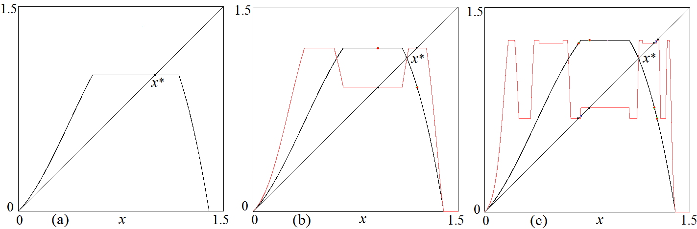
Figure 5: In (a) map $T_{\Delta}$ at $K=1$, superstable fixed point $x^{\ast}=K$. In (b) map $T_{\Delta}$ and its second iterate at $K=1.2$, superstable 2-cycle and unstable fixed point $x^{\ast}$. In (c) map $T_{\Delta}$ and its fourth iterate at $K=1.26$, superstable 4-cycle and unstable fixed point $x^{\ast}$.

When the fixed point $x^{\ast}$ exists, belonging to the decreasing branch (i.e. after the border collision), from piecewise smooth the map may become smooth. To detect this transition let us consider the critical point $x_{c}$ of $T_{\Delta}$ (point in which the derivative of $F_{\Delta}$ in (26) vanishes), where $x_{c}$ is given in (28). Then for $K<T_{\Delta}(x_{c})$ the map $T_{\Delta}$ has a horizontal flat branch (as it occurs in our example in Fig. 5), while for $K\geq T_{\Delta}(x_{c})$ the map is smooth (as it occurs in our example for $K=1.4)$.   

Notice that the two border points of the map $T_{\Delta}(x),$ bounding the flat branch, are given by the solutions of the equation $F_{\Delta}\left(x\right)=K,$ that is

$$x\left[1-\gamma x+\gamma x\tau\left(1-\frac{x}{N}\right)\right]=K$$

As long as the fixed point $x^{\ast}=K$ exists in the flat branch, the two border points are one smaller and one larger than $K$, while after its BCB (with the largest border point) the two border points are both smaller than $K$ (see Fig. 5).

After the BCB of the fixed point we can consider the second iterate of the map $T_{\Delta}^{2}(x)$ which, besides the unstable fixed point $x^{\ast}=N(1-\frac{1}{\tau})$, has a pair of superstable fixed points (related to the 2-cycle) which also undergo a border collision. The BCB of the fixed point of $T_{\Delta}^{2}$ can be studied in the same way as above for the fixed point of $T_{\Delta}.$ In particular, a sequence of period doubling BCBs (also called flip BCBs) occurs, leading to superstable cycles of period $2^{n}$.

In Fig. 5a the fixed point $x^{\ast}=K$ is still on the flat branch, while in Fig. 5b, after its BCB, we have a 2-cycle, and in Fig. 5c also the 2-cycle is unstable and a superstable 4-cycle exists, with periodic points $K$ and its first three iterates.

As $K$ increases, all the cycles existing in the complete U-sequence (see [18] and [13]) appear also here, either by saddle-node BCB or by flip BCB. For $T_{\Delta}(x)$ the cycles are either superstable or unstable. The superstable cycles occur as long as in the map a flat branch persists, that is, as remarked above in Property (5ii), as long as $K<T_{\Delta}(x_{c}),$ in which case the unstable cycles may belong to a chaotic repeller. While for $K>T_{\Delta}(x_{c})$ an invariant chaotic set may exist for the one-dimensional map $T_{\Delta}$ bounded by the critical point $T_{\Delta}(x_{c})$ and its images.

Going back to the two-dimensional map $T$ in the phase plane $(x_{1},x_{2})$, for $K<T_{\Delta}(x_{c})$ the one-dimensional map $T_{\Delta}(x)$ is piecewise smooth, and the attracting set for $T$ is some $n-$cycle on $\Delta$ having one (and necessarily only one) periodic point belonging to region $\Omega_{7}$ and its image is the point $(K,K).$ It follows that such an $n-$cycle is superstable also for the two-dimensional map $T$. However, it is not easy to predict the shape of its basin of attraction, as this attractor coexists with the fixed points on the two axes, and other attracting sets may exist in the phase plane outside $\Delta$. For example, for $K=1.2$, when an attracting 2-cycle exists, its basin of attraction is qualitatively similar to the one shown in Fig. 3a for the chaotic attractor. Differently it occurs for $K=1.2895$, when an attracting 3-cycle exists on the diagonal $\Delta$, but it is not the unique attractor with positive periodic points. In fact, it coexists with an attracting 4-cycle, born in pair with an unstable 4-cycle via saddle-node BCB, and the stable set of the unstable 4-cycle belongs to the frontier of the basins, shown in Fig. 6a.

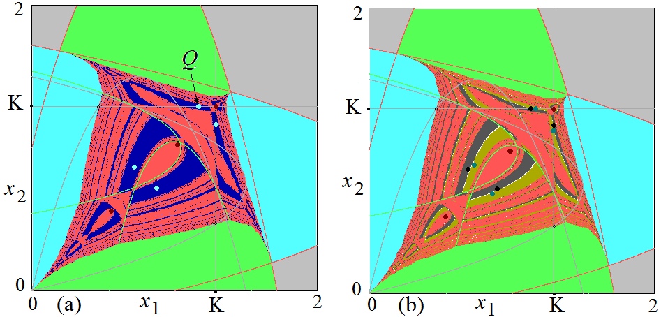
Figure 6: Basin of attraction of $\left(K,0\right)$ in green. Basin of attraction of $\left(0,K\right)$ in azure. Basin of attraction of $\left(0,0\right)$ in gray. Basin of attraction of the attractor lying on $x_{1}=x_{2}$ in red. In (a) $K=1.2895,$ the blue region is the basin of attraction of the 4-cycle. In (b) $K=1.29415,$ the dark-blue and dark-green regions are the basins of attraction of the two 4-cycles born by pitchfork bifurcation.

In order to investigate the stability and bifurcations of the 4-cycle we notice that, as already performed above, this can be done by use of a one dimensional map: the first return map on the straight line $x_{2}=K$ for $x_{1}>x_{1,m}=K\tau\left(1-\frac{K}{N}\right)$. So doing, it is possible to consider $T^{4}(x_{1},K)=(\psi(x_{1}),K)$ and the one-dimensional first return map $x_{1}(t+1)=\psi(x_{1}(t))$ has a stable fixed point in the range $[x_{1,m},K],$ corresponding to point $Q$ in Fig. 6a, with a positive eigenvalue. Increasing $K$ this fixed point undergoes a pitchfork bifurcation, leading to a pair of stable fixed points of $T^{4}$ which correspond to two stable 4-cycles for $T$ (see Fig. 6b). While the periodic points of the 4-cycles (one stable and one unstable) in Fig. 6a are symmetric with respect to $\Delta,$ those of the pair of stable 4-cycles existing after the pitchfork bifurcation are not symmetric themselves, but the two cycles have points which are pairwise symmetric with respect to $\Delta$ (as stated in Property-(4i)).

Remark. Notice that even if we have called the described bifurcation pitchfork, this term is proper only for the one-dimensional first return map on the straight line $x_{2}=K.$ In fact, let us reason as follows: considering the attracting 4-cycle before the bifurcation (as shown in Fig. 6a) we can see that two periodic points are in region $\Omega_{1},$ one in region $\Omega_{5}$ and one in region $\Omega_{9}$. Locally, in each point of the 4-cycle the map is smooth, and intuitively one can expect that the stability/instability of the 4-cycle depends on the eigenvalues of the Jacobian matrix of the map $T^{4}$ evaluated in any one of the four fixed points belonging to the 4-cycle of $T$, and obviously one eigenvalue is expected to be zero, due to the degeneracy of the map in regions $\Omega_{5}$ and $\Omega_{9}$. But this is not correct. The eigenvalue different from zero so determined, is not associated with the bifurcations of the 4-cycle. This is due to the degeneracy of the map: all the points of region $\Omega_{5}$ are mapped onto the straight line $x_{1}=K$ independently on the eigenvalues associated with the smooth map $T$ in points of this line belonging to region $\Omega_{1}.$ That is: the bifurcation associated with cycles must be determined by using the first return map, as we have done above, and not by using the standard tools which are correct for smooth systems (also locally).

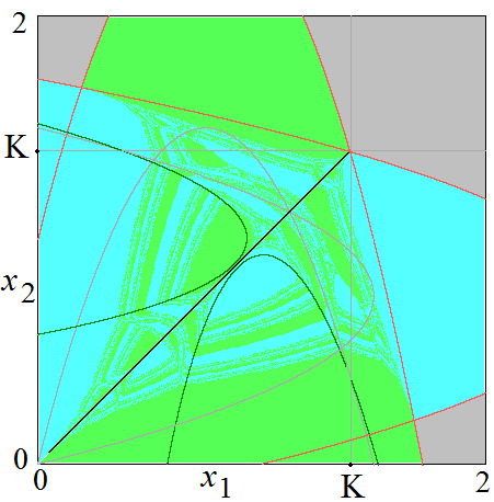
Figure 7: $K=1.4$ Basin of attraction of $\left(K,0\right)$ in green, basin of attraction of $\left(0,K\right)$ in azure, separated by a fractal frontier. The black dots along the line $x_{1}=x_{2}$ belong to a chaotic saddle.

Differently from the case $K<T_{\Delta}(x_{c})$, when a superstable cycles exists for $T$ on the diagonal of the phase plane, for $K>T_{\Delta}(x_{c})$ the one-dimensional map $T_{\Delta}(x)$ is smooth and an invariant set, which may be chaotic, exists on $\Delta$ but this invariant set may be not transversely attracting for the two-dimensional map $T$ in the phase plane $(x_{1},x_{2}).$ In fact, this can also be observed in our example at $K=1.4$: a chaotic interval exists on the diagonal $\Delta$, which is a chaotic repeller in the plane $\left(x_{1},x_{2}\right)$, the only attracting sets are the fixed points $(K,0)$ and $(0,K)$ on the axes, and their basins are separated by a fractal frontier, as shown in Fig. 7 (where the chaotic saddle is also evidenced by a black segment on $\Delta$). This may lead to a significant complexity in the socio-economic interpretation of the dynamics of the model. Indeed, given a generic value $(x_{1}(0),x_{2}(0))$ as initial condition it is hard to predict whether the states are ultimately converging to extinction of the first group or to extinction of the second group.

The analysis conducted till now for $K_{1}=K_{2}$ reveals the importance of the constraints for avoiding segregation. Indeed, from the dynamics of the model we know that if the number of the members of the two populations that are allowed to enter the system is sufficiently small, we always have a stable equilibrium of non segregation. On the contrary, as the maximum number of agents of the two groups that are allowed to enter the system increases, the equilibrium of non segregation loses its stability and a sequence of cycles of different periodicity appears. Further increasing this limit, we have that only equilibria of segregation are stable. This positive effect of the entry constraints on avoiding segregation can be explained observing that the reaction of agents of one group toward the presence of agents of the opposed group in the system is limited if the presence of the agents of both groups is small in number. In other words, the entry constraints avoid the problem of overshooting, which can be interpreted as impulsive and emotional behaviors.

3.2 Case $K_{1}\neq K_{2}$

Let us first describe some of the BCB curves observable in Fig. 4. The yellow region in the center of the figure is associated with the existence of the superstable fixed point $P=(K_{1},K_{2})\in\Omega_{7}.$ In our numerical simulations (in the given example) it is the only attractor coexisting with the fixed points on the axes, and its basin of attraction has a shape similar to the one shown in Fig. 3a (for the chaotic attractor). The boundaries of the yellow region in the two-dimensional bifurcation diagram in Fig. 4 are clearly curves of BCB, associated with a collision of $P$ with the borders $BC_{1,K}$ and $BC_{2,K}$ given in (7). The condition for the border collision is given by $P\in BC_{1,K}$ and $P\in BC_{2,K}$ leading to the BCB curves having the following equations:

$$BC_{e,1} :K_{2}=K_{1}\tau_{1}\left(1-\frac{K_{1}}{N_{1}}\right)\text{ at which }P=(K_{1},K_{2})\in BC_{1,K}$$ (29)

$$BC_{e,2} :K_{1}=K_{2}\tau_{2}\left(1-\frac{K_{2}}{N_{2}}\right)\text{ at which }P=(K_{1},K_{2})\in BC_{2,K}$$

which are drawn in Fig. 4. Notice that the intersection point of these two BCB curves, different from zero, is given by $K_{1}=K_{2}=N(1-\frac{1}{\tau})$ which corresponds to the BCB of the fixed point $K=N(1-\frac{1}{\tau})$ commented in Subsection 3.1. Let us consider the region with $K_{2}>K_{1}$, see Fig. 4. For parameters in the yellow region the fixed point $P$ is superstable. When a parameter point crosses these curves the fixed point $P$ either disappear by saddle-node BCB, when crossing $BC_{e,1},$ or enters (continuously) region $\Omega_{5}$ when crossing $BC_{e,2}.$ In our example, for parameters crossing $BC_{e,1}$ along the path $(j_{1})$ in Fig. 4, the fixed point $P$ merges with the unstable fixed point $P_{a}$ on the frontier of its basin of attraction and disappears, leaving the two fixed points on the axes as the only attractors. In Fig. 8a it is shown the phase plane before the bifurcation, and in Fig. 8b after the bifurcation, when $P_{a}$ becomes virtual and $(K_{1},K_{2})$ is no longer a fixed point. It can be seen that after the bifurcation, the former basin of $P$ is included in the basin of $\left(0,K_{2}\right).$

A similar bifurcation involving a 2-cycle is shown changing the parameters along the path $(j_{2})$ in Fig. 4. For low values of $K_{1}$ only the two fixed points on the axes are attracting (see Fig. 9a). Increasing $K_{1},$ a pair of 2-cycles appear by saddle-node BCB. Fig. 9b shows the phase plane very close to the bifurcation value, one of the pair of 2-cycles is attracting, with one periodic point in region $\Omega_{7}$ and one in region $\Omega_{1},$ while the saddle 2-cycle has periodic points in regions $\Omega_{9}$ and $\Omega_{1}$ (see Fig. 9c).

The occurrence of this saddle-node BCB bifurcation of the 2-cycle can also be determined analytically. In fact, considering the point $(K_{1},K_{2}),$ it must be a fixed point for the second iterate of map $T$. Thus let

$$F_{1}\left(K_{1},K_{2}\right) =K_{1}\left[1-\gamma_{1}K_{2}+\gamma_{1}\tau_{1}K_{1}\left(1-\frac{K_{1}}{N_{1}}\right)\right]$$ (30)

$$F_{2}\left(K_{1},K_{2}\right) =K_{2}\left[1-\gamma_{2}K_{1}+\gamma_{2}\tau_{2}K_{2}\left(1-\frac{K_{2}}{N_{2}}\right)\right]$$

the BCB curve satisfies the equation

$$F_{1}\left(F_{1}\left(K_{1},K_{2}\right),F_{2}\left(K_{1},K_{2}\right)\right)=K_{1}$$

that is:

$$F_{1}\left(K_{1},K_{2}\right)\left[1-\gamma_{1}F_{2}\left(K_{1},K_{2}\right)+\gamma_{1}\tau_{1}F_{1}\left(K_{1},K_{2}\right)\left(1-\frac{F_{1}\left(K_{1},K_{2}\right)}{N_{1}}\right)\right]=K_{1}$$

Notice that in Fig. 4 we have plotted the complete curves $BC_{e,1}$ and $BC_{e,2}$ as also the other parts, not bounding the region of a superstable fixed point, may be related to some border collision. Their effect may also be only of ”persistence border collision”, as it happens for example along the path $(j_{2})$ in Fig. 4: increasing $K_{1}$ the curve $BC_{e,1}$ is crossed, and the stable 2-cycle persists stable, but with periodic points in different regions (one point in $\Omega_{7}$ and one in region $\Omega_{9}).$

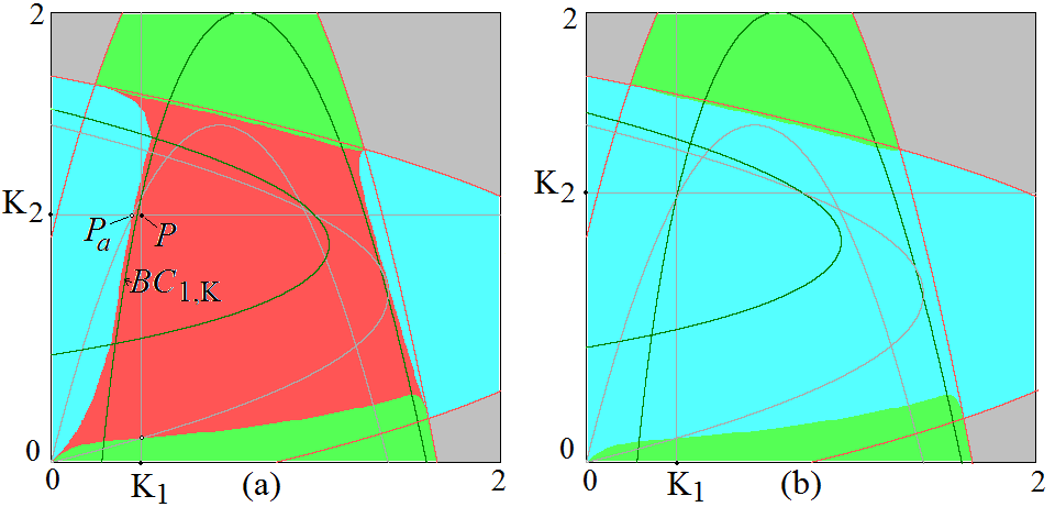
Figure 8: Bifurcation through $(j_{1})$, i.e. $K_{1}=0.4$. In (a) a superstable equilibrium, $P$, with basin in red, and a saddle, $P_{a}$, exist for $K_{2}=1.1$. In (b) for $K_{2}=1.2$ the equilibria $P$ and $P_{a}$ do not exist anymore as they disappeared by saddle-node BCB increasing $K_{2}$.

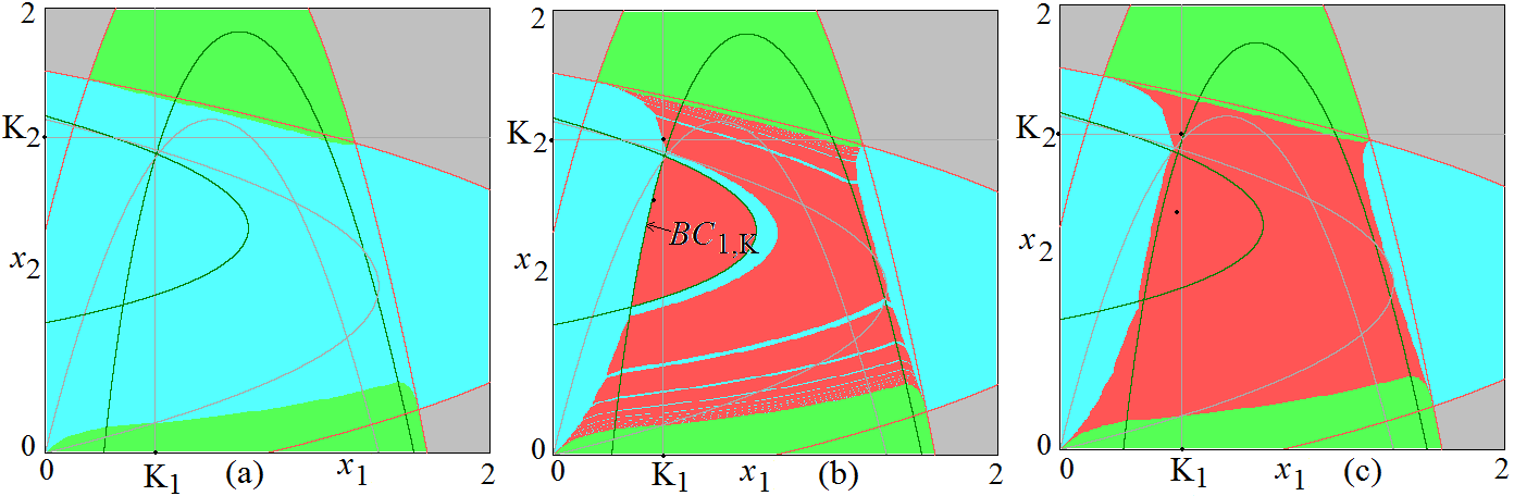
Figure 9: Bifurcation through $(j_{2}),$ $K_{2}=1.42$. In (a) $K_{1}=0.4936.$ In (b) $K_{1}=0.4937$. In (c) $K_{1}=0.55$. Basin of attraction of the 2-cycle in red.

In general, in order to predict the effect of the BCB of the fixed point, we can use the first return map along the straight line $x_{1}=K_{1}$ (considering the part above the diagonal in Fig. 4) and then make use of the skew tent map as the border collision normal form, evaluating the slopes of the functions at the border point, at the bifurcation values, as recalled in the previous sections. For example, crossing the curve $BC_{e,2}$ along the path $(j_{3})$ in Fig. 4 the fixed point $P$ crosses the curve $BC_{2,K}$ and enters region $\Omega_{5}$. The fixed point becomes unstable and a stable 2-cycle appears, having one periodic point in region $\Omega_{7}$ and one in region $\Omega_{5}$. In Fig. 10 it is shown the phase plane before the bifurcation, and in Fig. 10b the shape of the one-dimensional map restriction of $T$ on the straight line $x_{1}=K_{1},$ for $0\leq x_{2}\leq x_{2,m},$ given in (20) and (21), showing the superstable fixed point on the horizontal branch. The BCB of $P$ crossing the curve $BC_{2,K}$ in Fig. 10a corresponds to the BCB of the fixed point $x_{2}^{\ast}=K_{2}$ of the 1D map (20) in Fig. 10b. The slopes at the bifurcation value are one zero and one smaller than -1, thus the fixed point becomes unstable and a stable 2-cycle appears, as shown in Fig. 10c,d. We can see that the structure of the basins does not change.

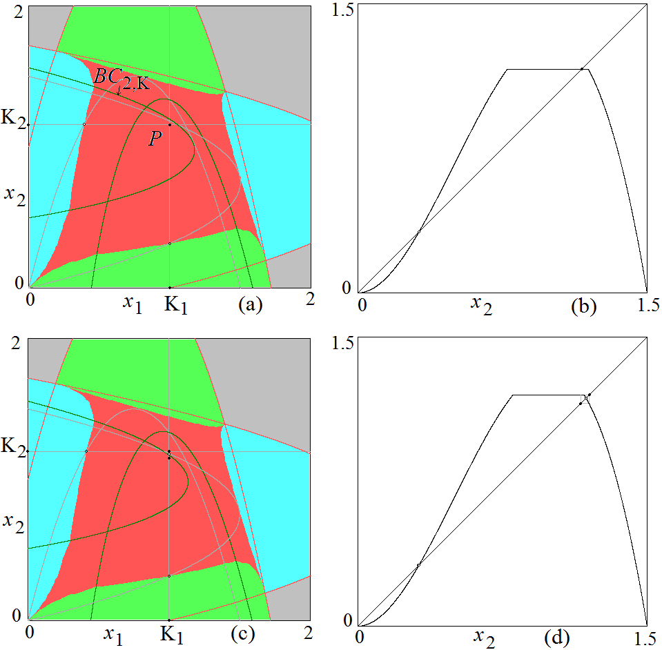
Figure 10: Bifurcation through $(j_{3})$, i.e. $K_{1}=1.$ In (a) and (b) $K_{2}=1.16$. In (a) the basin of attraction of $P=\left(K_{1},K_{2}\right)$ is in red. In (b) map $f_{2}\left(x_{2}\right)$ where black dot is the superstable equilibrium $x_{2}^{\ast}=K_{2}$. In (c) and (d) $K_{2}=1.2$, superstable 2-cycle appeared through a BCB of the fixed point $P$. In (c) basin of attraction of this 2-cycle in red. In (d) map $f_{2}\left(x_{2}\right)$ where the black dots are the 2-cycle. In (a) and (c) the black dots with while interior represent unstable equilibria.

Increasing $K_{2}$ along the path $(j_{3})$ in Fig. 4, the one-dimensional bifurcation diagram is reported in Fig. 11a. It can be seen that after the 2-cycle, also attracting cycles of period 4 and $2^{n}$ for any $n$ exist. This can be seen also in the enlargement of Fig. 4 reported in Fig. 11b. This region of the parameter plane corresponds to a region in which the BCBs lead to the appearance of all stable cycles in accordance with the U-sequence, as already remarked. In fact, the cycles there appearing all have one periodic point in the region $\Omega_{7}$ and the periodic points either belong all to the straight line $x_{1}=K_{1}$ (in which case the BCB can be studied via the restriction of $T$ on that line) or can be studied via the first return map on that line. All these cycles are superstable for these one-dimensional maps as well as for the two-dimensional map $T$, and undergo the border collisions. The periodicity regions observable in Fig. 11b are ordered according to the U-sequence.

Figure 11: In (a) 1D bifurcation diagram along $(j_{3})$, i.e. $K_{1}=1,$ and $K_{2}\in\left[1.15,1.35\right]$. The red segment represents the moment in which curve $BC_{p,2}$ is crossed. In (b) enlargement of the rectangle shown in Fig. 4.

From the enlargement in Fig. 11b it can be seen a change in the structure: the periodicity regions of the superstable cycles (on the left side) end, and a region with vertical strips appears. All the regions associated with superstable cycles on the left, according to the U-sequence, also have vertical strips on the right (still according with the U-sequence). This transition, which is typical for one-dimensional piecewise smooth maps with a horizontal branch, corresponds to the loss of the flat branch in the first return map or in the one-dimensional restriction representing the dynamics of the map $T$. In fact, as recalled above, the restriction of $T$ on the line $x_{1}=K_{1}$ has a horizontal branch as long as the cycles existing in the region characterized by the U-sequence have one periodic point in region $\Omega_{7}$. An example is shown in Fig. 10, and in Fig. 12a,b it is reported the map at the value of $K_{1}$ for which there is a superstable 4-cycle. Increasing $K_{1},$ a BCB occurs when the restriction of $T$ to the line $x_{1}=K_{1}$ becomes smooth, as shown in Fig. 12c,d.

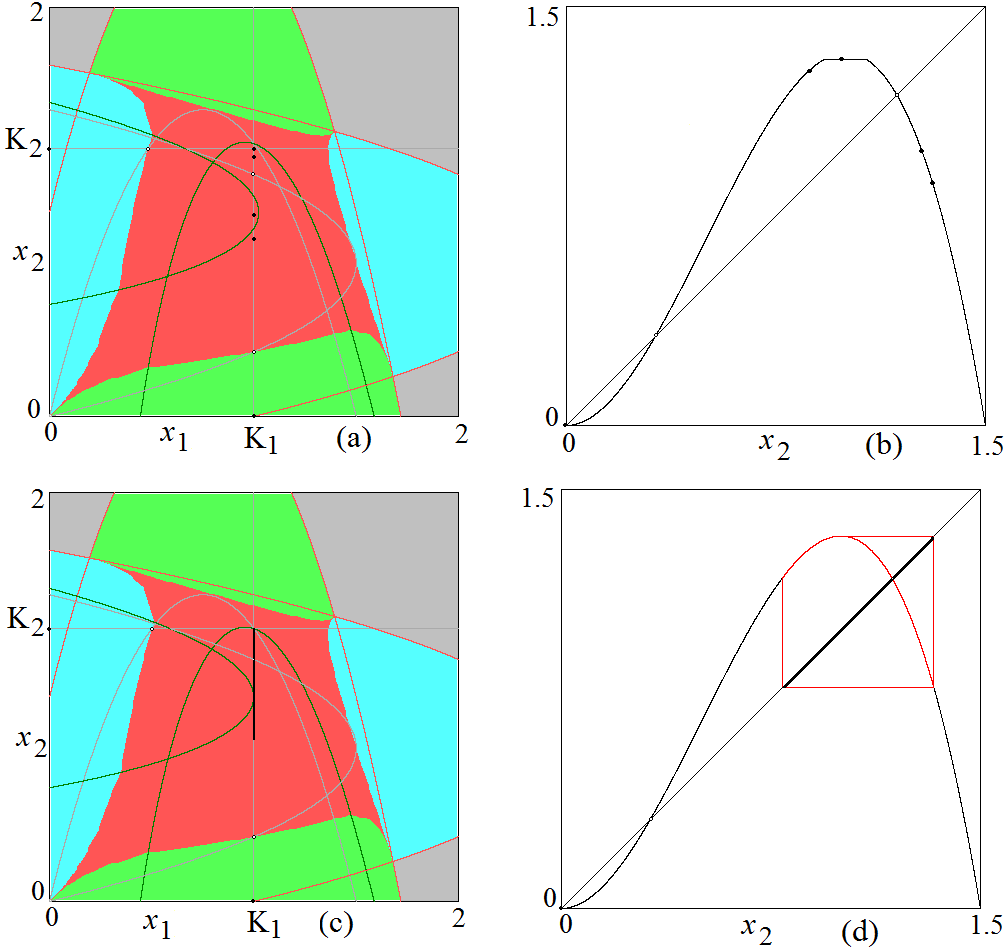
Figure 12: $K_{1}=1$. In (a) and (b) $K_{2}=1.31$. In (a) basin of attraction of the superstable 4-cycle (lying on $x_{1}=K_{1}$) in red. In (b) map $f_{2}\left(x_{2}\right)$ describing the dynamics of the model on the restriction $x_{1}=K_{1}$. In (c) and (d) $K_{2}=1.335$. In (c) basin of attraction of the chaotic attractor (lying on $x_{1}=K_{1}$) in red. In (d) map $f_{2}\left(x_{2}\right)$ which generates the chaotic attractor in (c).

In order to obtain the bifurcation curves in the parameter space $(K_{1},K_{2}),$ we proceed as follows. As recalled above, the restriction of map $T$ to the line $x_{1}=K_{1}$ is given in (20) and (21). The maximum of the function $F_{2}\left(K_{1},x_{2}\right),$ $\max_{x_{2}}\left\{F_{2}\left(K_{1},x_{2}\right)\right\}$, is obtained considering its proper critical point $x_{2,c}^{\ast},$ which satisfies $\frac{d}{dx_{2}}F_{2}\left(K_{1},x_{2,c}^{\ast}\right)=0,$ where the first derivative is given in (22), and the value in the critical point (i.e. $\max_{x_{2}}\left\{F_{2}\left(K_{1},x_{2}\right)\right\}=F_{2}\left(K_{1},x_{2,c}^{\ast}\right))$. Via standard computations we get

$$x_{2,c}^{\ast}=\frac{N_{2}}{3}+\left[\left(\frac{N_{2}}{3}\right)^{2}+\frac{N_{2}}{3\gamma_{2}\tau_{2}}\left(1-\gamma_{2}K_{1}\right)\right]^{1/2}$$

so that the maximum of the function $F_{2}\left(K_{1},x_{2}\right)$ is given by

$$F_{2}\left(K_{1},x_{2,c}^{\ast}\right)=\left(x_{2,c}^{\ast}\right)^{2}\left(2\frac{x_{2,c}^{\ast}}{N_{2}}-1\right)\gamma_{2}\tau_{2}$$

Then a BCB occurs when this maximum reaches the constraint on $x_{2},$ which is the value $K_{2},$ and thus is determined by the condition $K_{2}=F_{2}\left(K_{1},x_{2,c}^{\ast}\right)$ which leads to the following BCB curve in the parameter space:

$$BC_{p,2}:K_{2}=\left(x_{2,c}^{\ast}\right)^{2}\left(2\frac{x_{2,c}^{\ast}}{N_{2}}-1\right)\gamma_{2}\tau_{2}$$ (31)

A portion of this curve is shown in Fig. 4 and in the enlargement, in Fig. 11b.

The other BCB due to the restriction on the straight line $x_{2}=K_{2}$ is determined similarly, considering (17) and (18). The maximum of the function $F_{1}\left(x_{1},K_{2}\right)$ given in (18) is $\max_{x_{1}}\left\{F_{1}\left(x_{1},K_{2}\right)\right\}=F_{1}\left(x_{1,c}^{\ast},K_{2}\right)$, where $x_{1,c}^{\ast}$ is the proper critical point, a solution of $\frac{d}{dx_{1}}F_{1}\left(x_{1},K_{2}\right)=0.$ From the first derivative given in (19) we get

$$x_{1,c}^{\ast}=\frac{N_{1}}{3}+\left[\left(\frac{N_{1}}{3}\right)^{2}+\frac{N_{1}}{3\gamma_{1}\tau_{1}}\left(1-\gamma_{1}K_{2}\right)\right]^{1/2}$$

so that the maximum of the function is given by

$$F_{1}\left(x_{1,c}^{\ast},K_{2}\right)=\left(x_{1,c}^{\ast}\right)^{2}\left(2\frac{x_{1,c}^{\ast}}{N_{1}}-1\right)\gamma_{1}\tau_{1}$$

A BCB occurs when this maximum reaches the value $K_{1},$ and thus is determined by the condition $K_{1}=F_{1}\left(x_{1,c}^{\ast},K_{2}\right)$ which leads to the following BCB curve in the parameter space:

$$BC_{p,1}:K_{1}=\left(x_{1,c}^{\ast}\right)^{2}\left(2\frac{x_{1,c}^{\ast}}{N_{1}}-1\right)\gamma_{1}\tau_{1}$$ (32)

In Fig. 4 a portion of both bifurcation curves $BC_{p,1}$ and $BC_{p,2}$ are shown, and better visible is $BC_{p,2}$ in the enlargement in Fig. 11b. From the two-dimensional bifurcation diagram we can see that the BCB occurring crossing the curve $BC_{e,1}$ leads to persistence, while its portion in the region with vertical strips is no longer a bifurcation, as the restriction to the one-dimensional map is smooth and the point $(K_{1},K_{2})$ does not belong to the attracting set.

Differently, the crossing of the curve $BC_{p,2}$ leading to a smooth restriction, determines the transition from a piecewise-smooth (with a flat branch) to a smooth map. It is worth to note that each periodicity region associated with a superstable cycle, on the left side of the curve $BC_{p,2},$ leads to a correspondent vertical strip associated with an attracting cycle on its right side. On the left side of the curve $BC_{p,2}$ the periodicity regions of superstable cycles have as limit sets curves related with homoclinic bifurcations, which also leads to correspondent vertical lines associated with chaotic dynamics on the right side (when the map is smooth).

In order to illustrate the dynamics of $T$ in this parameter region we consider two more paths, at $K_{2}=1.48$ and at $K_{2}=1.37$ which also are evidenced in Fig. 4 and Fig. 11b, and describe some bifurcations occurring as $K_{1}$ increases.

Let us start considering $K_{2}=1.48$ fixed. From Fig. 11b we can see that increasing $K_{1}$ first the BCB crossing $BC_{e,1}$ occurs, and then the crossing of $BC_{p,2}$. The one-dimensional bifurcation diagram as a function of $K_{1}$ is shown in Fig. 13a. In the region where the dynamics are represented by the U-sequence as commented above, the effect of the crossing of $BC_{e,1}$ (which occurs approximately at $K_{1}=0.83)$ corresponds to a persistence of the attracting cycle: before the bifurcation the superstable cycles have one periodic point in region $\Omega_{7}$ and all others in region $\Omega_{5}$ while after the bifurcation the periodic point $(K_{1},K_{2})$ belongs to region $\Omega_{1},$ its preimage to region $\Omega_{7}$ and all others in region $\Omega_{5}$. Then, increasing $K_{1}$ the crossing of $BC_{p,2}$ occurs (approximately at $K_{1}=0.855),$ and this leads to a smooth shape of the first return map on $x_{1}=K_{1}$ (as above in Fig. 12d). The attracting set on this line seems a large invariant chaotic interval, as shown in Fig. 13c. Notice that after this bifurcation, the corner point $(K_{1},K_{2})$ (belonging to region $\Omega_{1}$) does not belong to the attracting set. This fact may lead to changes in the structure of the basins of attraction of the attracting sets. As an example, in Fig. 13c the corner point is very close to the boundary separating the basin of the chaotic attractor from the basin of the fixed point $(K_{1},0)$. In Fig. 13d (at $K_{1}=0.9$) we are at the contact: the corner point belongs to the boundary of the basin of $(K_{1},0),$ as in fact the complete region $\Omega_{7}$ which is mapped into $P$, now belongs to the basin of $(K_{1},0)$ together with all its preimages of any rank. Increasing $K_{1}$ the attractor (a cycle or a chaotic attractor) takes a more complex shape in the two-dimensional phase plane: the dynamics can still be studied by using the first return map on the line $x_{1}=K_{1}$ but the number of points of a trajectory outside the line changes at each iteration so that it is difficult to have it analytically, even in implicit form (an example is shown in Fig. 13e). In Fig. 11b we also have evidenced the point related to the ”final bifurcation”, as the positive attractor (here chaotic) has a contact with the boundary of its basin of attraction (see Fig. 13f at $K_{1}=1.198$). After it is transformed into a chaotic repeller, leaving only the two attracting fixed points on the axes, with a basin of attraction having a fractal structure (similar to the one shown above in Fig. 7).

Let us now consider $K_{2}=1.37$ fixed. The one-dimensional bifurcation diagram as a function of $K_{1}$ is shown in Fig. 14a. From the region where the dynamics are associated with superstable cycles and the U-sequence, the BCB crossing $BC_{p,2}$ occurs approximately at $K_{1}=0.963,$ leading to a chaotic attractor, which completely belongs to the line $x_{1}=K_{1}$ even if after the bifurcation the point $(K_{1},K_{2})$ no longer belongs to the attractor. The crossing of $BC_{e,1},$ which here occurs approximately at $K_{1}=0.975,$ does not represent a bifurcation, it denotes only the transition of the corner point $(K_{1},K_{2})$ from region $\Omega_{5}$ to region $\Omega_{1}$. Increasing $K_{1}$ it can be noticed another region in which the dynamics are again described by superstable cycles in the U-sequence structure. This transition happens when the existing attractor has a contact, i.e. a border collision, with the boundary of region $\Omega_{7}.$ In our example this occurs approximately at $K_{1}=1.185$ as shown in Fig. 14b. After the contact the attractor is a superstable cycle with one periodic point in region $\Omega_{7}$ and thus it is mapped into $P=(K_{1},K_{2})$ which is again a periodic point, an example is shown in Fig. 14c. The ”final bifurcation” of this attractor happens when the periodic point $P=(K_{1},K_{2})$ has a contact with its basin boundary, which occurs approximately at the value $K_{1}=1.245$ shown in Fig. 14c: on the other side of the contact point there is the basin of the fixed point $(K_{1},0$) so that after the bifurcation the attractors are only the fixed points on the axes, and the basin of $(K_{1},0$) increases, as shown in Fig. 14d ($K_{1}=1.246$).

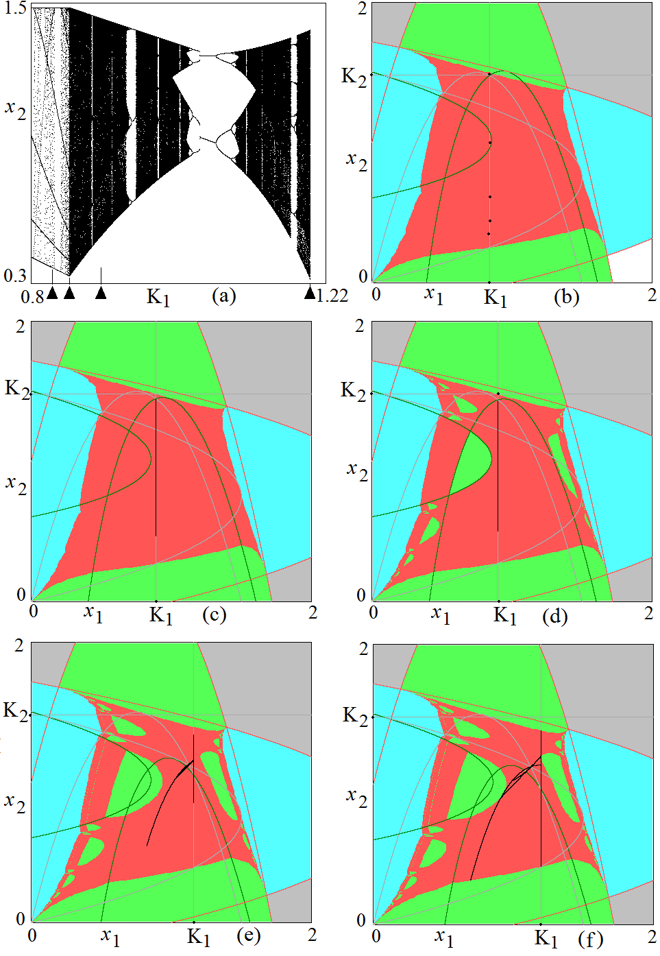
Figure 13: $K_{2}=1.48$. In (a) 1D bifurcation diagram for $K_{1}\in\left[0.8,1.22\right]$. In (b) basins of attraction and attractors for $K_{1}=0.84$. In (c) basins of attraction and attractors for $K_{1}=0.89$. In (d) basins of attraction and attractors for $K_{1}=0.9$, here the corner point $\left(K_{1},K_{2}\right)$ is marked with a black dot for highlighting that it enters the basin of attraction of $\left(K_{1},0\right)$, i.e. the green region. In (e) basins of attractions and attractors for $K_{1}=1.16$. In (f) basins of attraction and attractors for $K_{1}=1.198$.

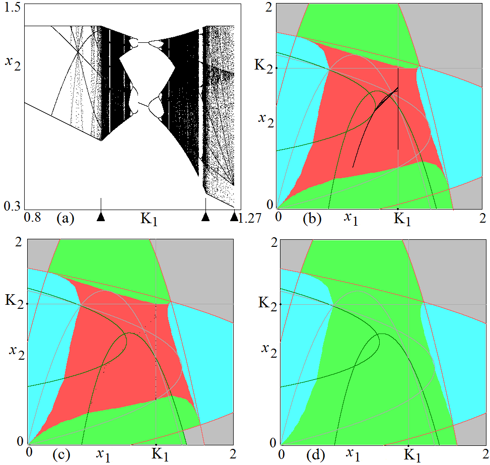
Figure 14: $K_{2}=1.37$. In (a) 1D bifurcation diagram for $K_{1}\in\left[0.8,1.27\right]$. In (b) basins of attraction and attractors for $K_{1}=1.185$. In (c) basins of attraction and attractors for $K_{1}=1.245$, the cycle in the red region is superstable. In (d) basins of attraction and attractors for $K_{1}=1.246$.

For what concerns the implications of the entry constraints, $K_{1}$ and $K_{2}$, in terms of segregation, the analysis conducted in this section reveals that the effects of these entry constraints change if we make a strong discrimination on the maximum number of agents allowed to enter the system between the two groups. Indeed, if the difference between $K_{i}$ and $K_{j}$ is sufficiently large, with $K_{i}$ near to $N_{i}$ and $K_{j}$ small, then we will have only stable equilibria of segregation. Moreover, starting with $K_{i}$ relatively large and increasing $K_{j}$, a stable equilibrium of non segregation cannot be reached, but rather an attractor in which the number of agents of the two groups that enter and exit the system fluctuates over time and when $K_{j}$ becomes sufficiently large again only an equilibrium of segregation is possible. This reveals an important aspect of the issue of segregation, i.e. to avoid overreaction of the two groups toward segregation we need to limit in a similar way the number of possible entrances of both types of agents in the system.

4 Conclusions

In this work we have analyzed the effects of several constraints on the dynamics of the adaptive model of segregation proposed in [3]. The constraints represent the maximum number of agents of two different groups that are allowed to enter a system. We have provided an accurate and deep investigation of the dynamics in the symmetric case, i.e. when the two groups of agents that differ for a specific feature are of the same size and have the same level of tolerance. The definition of the two-dimensional piecewise smooth map lead to a map with different definitions in several partitions. Besides the existence of two stable segregation equilibria on the axes, we have shown that other attractors may exist, regular or chaotic. The effect of the constraints, modifying the regions, leads to border collision bifurcations of the positive attracting sets. In the $\left(K_{1},K_{2}\right)$-parameter plane of the constraints, we have detected several BCB curves, explaining their effects on the dynamic behaviors. The results are obtained by using several first return maps on suitable intervals, and making use of the bifurcation theory for one-dimensional piecewise smooth maps. A deep investigation of the effects of the constraints when the symmetry is broken is desirable and can reveal dynamics not observable in the symmetric setting. This line of research is left for further studies.

References

- [1] V. Avrutin, B. Futter, and M. Schanz. The discontinuous top tent map and the nested period incrementing bifurcation structure. Chaos, Solitons & Fractals, 45:465–482, 2012.
- [2] G. I. Bischi, L. Gardini, and U. Merlone. Impulsivity in binary choices and the emergence of periodicity. Discrete Dynamics in Nature and Society, Volume 2009, 2009.
- [3] G. I. Bischi and U. Merlone. Nonlinear economic dynamics, chapter An Adaptive dynamic model of segregation, pages 191–205. Nova Science Publisher, New York, 2011.
- [4] S. Brianzoni, E. Michetti, and I. Sushko. Border collision bifurcations of superstable cycles in a one-dimensional piecewise smooth map. Mathematics and Computers in Simulation, 81(1):52–61, 2010.
- [5] G. I. Bischi C. Chiarella, M. Kopel, and F. Szidarovszky. Nonlinear oligopolies: Stability and bifurcations. Heidelberg: Springer., 2009.
- [6] A. Dal Forno, L. Gardini, and U. Merlone. Ternary choices in repeated games and border collision bifurcations. Chaos Solitons and Fractals, in press doi: 10.1016/j.chaos.2011.12.003, 2012.
- [7] R. Day. Complex Economic Dynamics. MIT Press, Cambridge, 1994.
- [8] R. Day and P. Chen. Nonlinear Dynamics and Evolutionary Economics, chapter Chaotically switching bear and bull markets: the derivation of stock price distributions from behavioral rules, pages 169–182. Oxford University Press, Oxford, 1993.
- [9] M. di Bernardo, C. J. Budd, A. R. Champneys, and P. Kowalczyk. Piecewise-smooth Dynamical Systems: Theory and Applications. Springer-Verlag, Berlin, 2008.
- [10] J. M. Epstein and R. L. Axtell. Growing Artificial Societies: Social Science from the Bottom up. Growing Artificial Societies: Social Science from the Bottom up.
- [11] L. Gardini, U. Merlone, and F. Tramontana. Inertia in binary choices: Continuity breaking and big-bang bifurcation points. Journal of Economic Behavior & Organization, 80(1):153–167, 2011.
- [12] L. Gardini, I. Sushko, and A. Naimzada. Growing through chaotic intervals. Journal of Economic Theory, 143:541–557, 2008.
- [13] B. L. Hao. Elementary Symbolic Dynamics and Chaos in Dissipative Systems. World Scientific, Singapore, 1989.
- [14] C. Hommes and H. Nusse. “Period three to period two”bifurcation for piecewise linear models. Journal of Economics, 54(2):157–169, 1991.
- [15] S. Ito, S. Tanaka, and H. Nakada. On unimodal transformations and chaos II. Tokyo Journal of Mathematics, 2:241–259, 1979.
- [16] K. Matsuyama. The good, the bad, and the ugly: An inquiry into the causes and nature of credit cycles. Center for Mathematical Studies in Economics and Management. Science Discussion Paper No.1391, Northwestern University., 2011.
- [17] Yu. L. Mas̆trenko, V. L. Mas̆trenko, and L. O. Chua. Cycles of chaotic intervals in a time-delayed Chua’s circuit. International Journal of Bifurcation and Chaos in Applied Sciences and Engineering, 3(6):1557–1572, 1993.
- [18] N. Metropolis, M. L. Stein, and P. R. Stein. On finite limit sets for transformations on the unit interval. J. Comb. Theory, 15:25–44, 1973.
- [19] H. E. Nusse and J. A. Yorke. Border-collision bifurcations including “period two to period three”for piecewise smooth systems. Physica D, 57(1–2):39–57, 1992.
- [20] H. E. Nusse and J. A. Yorke. Border-collision bifurcations for piecewise smooth one-dimensional maps. International Journal of Bifurcation and Chaos in Applied Sciences and Engineering, 5(1):189–207, 1995.
- [21] T. Puu and I. Sushko. Oligopoly Dynamics, Models and Tools. Springer Verlag, New York., 2002.
- [22] T. Puu and I. Sushko. Business Cycle Dynamics, Models and Tools. Springer Verlag, New York., 2006.
- [23] T. C. Schelling. Models of segregation. The American Economic Review, 59(2):488–493, 1969.
- [24] I. Sushko, A. Agliari, and L. Gardini. Bifurcation structure of parameter plane for a family of unimodal piecewise smooth maps: border-collision bifurcation curves. Chaos, Solitons & Fractals, 29(3):756–770, 2006.
- [25] I. Sushko and L. Gardini. Degenerate bifurcations and border collisions in piecewise smooth 1d and 2d maps. International Journal of Bifurcation and Chaos, 20:2045–2070, 2010.
- [26] I. Sushko, L. Gardini, and K. Matsuyama. “superstable credit cycles and u-sequence”. Chaos Solitons & Fractals, 59:13–27, 2014.
- [27] F. Tramontana, L. Gardini, and T. Puu. Mathematical properties of a combined cournot-stackelberg model. Chaos, Solitons & Fractals, 44:58–70, 2011.
- [28] F. Tramontana, L. Gardini, and F. Westerhoff. Heterogeneous Speculators and Asset Price Dynamics: Further Results from a One-Dimensional Discontinuous Piecewise-Linear Map. Computational Economics, 38(3):329–347, 2011.
- [29] F. Tramontana, F. Westerhoff, and L. Gardini. On the complicated price dynamics of a simple one-dimensional discontinuous financial market model with heterogeneous interacting traders. Journal of Economic Behavior & Organization, 74(3):187–205, 2010.
- [30] J. Zhang. Residential segregation in an all-integrationist world. Journal of Economic Behavior and Organization, 54:533–550, 2004.
- [31] Z. T. Zhusubaliyev and E. Mosekilde. Bifurcations and Chaos in Piecewise-Smooth Dynamical Systems. World Scientific, River Edge, NJ, 2003.