Büchi Determinization Made Tighter

Abstract

By separating the principal acceptance mechanism from the concrete acceptance condition of a given Büchi automaton with $n$ states, Schewe presented the construction of an equivalent deterministic Rabin transition automaton with $o((1.65n)^{n})$ states via history trees, which can be simply translated to a standard Rabin automaton with $o((2.66n)^{n})$ states. Apart from the inherent simplicity, Schewe’s construction improved Safra’s construction (which requires $12^{n}n^{2n}$ states). However, the price that is paid is the use of at most $2^{n-1}$ Rabin pairs (instead of $n$ in Safra’s construction). So, whether the index complexity of Schewe’s construction can be improved is an interesting problem. In this paper, we improve Schewe’s construction to $2^{\lceil(n-1)/2\rceil}$ Rabin pairs with the same state complexity. We show that when keeping the state complexity, the index complexity of proposed construction is tight already.

I Introduction

The theory of automata over infinite words underpins much of formal verification. In automata-based model checking [1, 2], to decide whether a given system described by an automaton satisfies a desired property specified by a Büchi automaton [3], one constructs the intersection of the system automaton with the complementation of the property automaton, and checks its emptiness [1, 2]. To complement Büchi automata, Rabin, Muller, Parity as well as Streett automata [4] are often involved, since deterministic Büchi automata are not closed under complementation. Recently, co-Büchi automata have attracted much attention because of its simplicity and its surprising utility [5, 6, 7]. Further, in LTL model checking, the transformation from LTL formulas to Büchi automata is a key procedure, where generalized Büchi automata are often used as an intermediary [1, 2].

Büchi automata were first introduced as a tool for proving the decidability of monadic second order logic of one successor (S1S) [3]. They are nearly the same as finite state automata except for the acceptance condition: a run of a finite state automaton is accepting if a final state is visited at the end of the run, whereas a run of a Büchi automaton is accepted if a final state is visited infinitely often. This small difference enables Büchi automata to accept infinite sequences instead of finite ones. However, the close relationship between finite state and Büchi automata does not mean that automata manipulations of Büchi automata are as simple as those for finite state automata [8]. In particular, Büchi automata are not closed under determinization. For a non-deterministic Büchi automaton, there might not exist a deterministic Büchi automaton that accepts the same language as the non-deterministic one does. That is, deterministic Büchi automata are strictly less expressive than the nondeterministic ones; while for a finite state automaton, a simple subset construction is sufficient for efficient determinization [8]. Determinization of Büchi automata requires automata with more complicated acceptance mechanisms, such as automata with Muller’s subset condition [12, 13], Rabin and Streett’s accepting pair conditions [9, 10], or Parity acceptance condition [11, 15], and so forth.

Besides the close relation with complementation, determinization is also useful in solving games and synthesizing strategies. The first determinization construction for Büchi automata was introduced by McNaughton by converting nondeterministic Büchi automata to deterministic Muller automata with a doubly exponential blow-up [10]. Safra achieved an asymptotically optimal determinization algorithm using Safra trees [9]. His method extends the powerset construction by branching out a new computation path each time the given automaton reaches a final state. Thus the states of the resulting automaton are not a set of states but a set of tree structures. Safra’s construction transforms a nondeterministic Büchi automaton with $n$ states into a deterministic Rabin automaton with $12^{n}n^{2n}$ states and $n$ Rabin pairs. Piterman [11] presented a tighter construction by utilizing compact Safra trees which are obtained by using a dynamic naming technique throughout the construction of Safra trees. With compact Safra trees, a nondeterministic Büchi automaton can be transformed into an equivalent deterministic parity automaton with $2n^{n}n!$ states and $2n$ priorities (can be equivalently transformed to a deterministic Rabin automaton with the same complexity and $n$ priorities). The advantage of Piterman’s determinization is to output deterministic Parity automata which is easier to manipulate.

By separating the principal acceptance mechanism from the concrete acceptance condition of a Büchi automaton with $n$ states, Schewe presented the construction of an equivalent deterministic Rabin transition automaton with $o((1.65n)^{n})$ states, which can be simply translated to a standard Rabin automaton with $o((2.66n)^{n})$ states [15]. Based on this construction, Schewe also obtained an $O((n!)^{2})$ transformation from Büchi automata to deterministic parity automata that actually resembles Piterman’s construction (Liu and Wang [14] independently present a similar state complexity result to Piterman’s determinization). Schewe’s construction is mainly based on a new data structure, namely, history tree which is an ordered tree with labels. Compared to Safra’s construction (whose complexity engendered a line of expository work), Schewe’s construction is simple and intuitive. Subsequently, a lower bound for the transformation from Büchi automata to deterministic Rabin transition automata is proved to be $O((1.64n)^{n})$ [17]. Therefore the state complexity for Schewe’s construction of Rabin transition automata is optimal. For the ordinary Rabin acceptance condition, the construction via history trees also conducts the best upper-bound complexity result $o((2.66n)^{n})$. However, the price paid for that is the use of $2^{n-1}$ Rabin pairs (instead of $n$ in Safra’s construction). Therefore, whether the index complexity of Schewe’s construction can be improved is an interesting problem.

With this motivation, we reconstruct history trees as history trees with canonical identifiers by adding an extra unique identifier on each node of the tree. To reduce the index complexity and keep the state complexity meanwhile, it is required that whenever a node $\tau$ occurs in a history tree, its identifer must keep the same with the one used in other history trees where $\tau$ occurs. We show that it is possible to keep each $\tau$, in the history trees throughout the determinization construction, annotated by the same identifer ranging over $2^{\lceil(n-1)/2\rceil}$ different identifiers. As a consequence, improved constructions of deterministic Rabin transition automata and ordinary Rabin automata are obtained which have the same state complexity as Schewe’s construction but reduces the index complexity to $2^{\lceil(n-1)/2\rceil}$. We also show that when keeping the state complexity, the index complexity of the proposed construction is tight already.

The rest of the paper is organized as follows. The next section briefly introduces automata over infinite words. In Section III, Schewe’s construction of deterministic Rabin automata based on history trees is presented. In section IV, the main data structure history trees with canonical identifiers is presented. In the sequel, our improved constructions of deterministic Rabin transition automata and ordinary deterministic Rabin automata are presented in Section V and VI, respectively.

II Automata

Let $\Sigma$ denote a finite set of symbols called an alphabet. An infinite word $\alpha$ is an infinite sequence of symbols from $\Sigma$. $\Sigma^{\omega}$ is the set of all infinite words over $\Sigma$. We present $\alpha$ as a function $\alpha:\mathbb{N}\rightarrow\Sigma$, where $\mathbb{N}$ is the set of non-negative integers. Thus, $\alpha(i)$ denotes the letter appearing at the $i^{th}$ position of the word. In general, $\mathsf{Inf}(\alpha)$ denotes the set of symbols from $\Sigma$ which occur infinitely often in $\alpha$. Formally,

$$\mathsf{Inf}(\alpha)=\{\sigma\in\Sigma\mid\exists^{\omega}n\in\mathbb{N}:\alpha(n)=\sigma\}$$

Note that $\exists^{\omega}n\in\mathbb{N}$ means there exist infinitely many $n$ in $\mathbb{N}$.

Definition 1 (Automata)

An automaton over $\Sigma$ is a tuple $A=(\Sigma,Q,\delta,Q_{0},\lambda)$, where $Q$ is a non-empty, finite set of states, $Q_{0}\subseteq Q$ is a set of initial states, ${\delta}\subseteq Q\times\Sigma\times Q$ is a transition relation, and $\lambda$ an acceptance condition. $\blacksquare$

A run $\rho$ of an automaton $A$ on an infinite word $\alpha$ is an infinite sequence $\rho:\mathbb{N}\rightarrow Q$ such that $\rho(0)\in Q_{0}$ and for all $i\in\mathbb{N}$, $(\rho(i),\alpha(i),\rho(i+1))\in{\delta}$. $A$ is said deterministic if $I$ is a singleton, and for any $(q,\sigma,q^{\prime})\in$ $\delta$, there exists no $(q,\sigma,q^{\prime\prime})\in\delta$ such that $q^{\prime\prime}=q^{\prime}$, and non-deterministic otherwise. Similar to infinite words, $\mathsf{Inf}(\rho)$ denotes the set of states from $Q$ which occur infinitely often in $\rho$. Formally,

$$\mathsf{Inf}(\rho)=\{q\mid\exists^{\omega}n\in\mathbb{N}:\rho(n)=q\}$$

Several acceptance conditions are studied in literature. We present three of them here:

• Büchi, where $\lambda\subseteq Q$, and $\rho$ is accepted iff $\mathsf{Inf}(\rho)\cap\lambda\not=\emptyset$.

• Parity, where $\lambda=\{\lambda_{1},\lambda_{2},\ldots,\lambda_{2k}\}$ with $\lambda_{1}\subset\lambda_{2}\subset\ldots\subset\lambda_{2k}=Q$, and $\rho$ is accepted if the minimal index $i$ for which $\mathsf{Inf}(\rho)\cap\lambda_{i}\not=\emptyset$ is even.

• Rabin, where $\lambda=\{(\lambda_{1},\beta_{1}),(\lambda_{2},\beta_{2}),\ldots,(\lambda_{k},\beta_{k})\}$ with $\lambda_{i}$, $\beta_{i}\subseteq Q$ and $\rho$ is accepted iff for some $1\leq i\leq k$, we have that $\mathsf{Inf}(\rho)\cap\lambda_{i}\not=\emptyset$ and $\mathsf{Inf}(\rho)\cap\beta_{i}=\emptyset$.

An automaton accepts a word if it has an accepted run on it. The accepted language of an automaton $A$, denoted by $L(A)$, is the set of words that $A$ accepts.

We denote the different types of automata by three letter acronyms in $\{D,N\}\times\{B,P,R\}\times\{W\}$. The first letter stands for the branching mode of the automaton (deterministic or nondeterministic); the second letter stands for the acceptance condition type (Büchi, parity, or Rabin); and the third letter indicates that the automaton runs on words. While acceptance condition of an ordinary automaton is defined on states, the acceptance condition of a transition automaton is defined on transitions of the automaton. Accordingly, with respect to each type of ordinary automata, we also have its transition version.

III Determinization via History Trees

This section presents Schewe’s determinization via history trees [15].

III-A History Trees

A history tree is a simplification of a Safra tree [9] by the omission of explicit names for nodes. It is actually an ordered tree with labels.

Let $\mathbb{N}_{{>}0}$ be the set of positive integers. An ordered tree $T\subseteq\mathbb{N}_{{>}0}^{*}$ is a finite, prefix-closed and order-closed (with respect to siblings) subset of finite sequences of positive integers. That is, if a sequence $\tau=t_{0}t_{1}\ldots t_{n}$ is in $T$, then all proper prefixes of $\tau$, $\tau^{\prime}=t_{0}t_{1}\ldots t_{m}$, $m<n$, concatenated with $s$ where $s=\epsilon$ or $s\in\{1,\cdots,t_{m+1}-1\}$ are also in $T$. For a node $\tau$ of an ordered tree $T$, we call the number of children of $\tau$ its degree, denoted by $deg_{T}(\tau)=|\{i\in\mathbb{N}_{{>}0}\mid\tau\cdot i\in T\}|$.

Notice that a tree is not order-closed if, and only if, there exists at least one node $x_{1}\ldots x_{n-1}x_{n}$ in the tree such that $x_{n}\geq 2$ and $x_{1}\ldots x_{n-1}(x_{n}-1)$ is not in the tree. We call such a node an imbalanced node. Further, the greatest order-closed subset of a tree is called the set of stable nodes; and the other nodes are called unstable nodes. Intuitively, if $x_{1}\ldots x_{n-1}x_{n}$ where $n\geq 1$ is an imbalanced node, all nodes $x_{1}\ldots x_{n-1}x$ where $x\geq x_{n}$, and their descendants, are unstable nodes.

Definition 2 (History Trees [15])

A history tree for a given nondeterministic Büchi automaton $A=(\Sigma,Q,Q_{0},\delta,$ $\lambda)$ is a labelled tree $\langle T,l\rangle$, where $T$ is an ordered tree, and $l:T\rightarrow 2^{Q}\setminus\{\emptyset\}$ is a labeling function that maps the nodes of $T$ to non-empty subsets of $Q$, such that the following three properties hold:

• P1: the label of each node is non-empty,

• P2: the labels of different children of a node are disjoint, and

• P3: the label of each node is a proper superset of the union of the labels of its children. $\blacksquare$

Notice that in a history tree, all the nodes are not explicitly named, but an implicit name (derived from the underlying ordered tree) is used. Fig. 1 shows an example of history tree where the implicit names of nodes are written in red. $a$, $b$, $c$, $d$, $e$, $f$, and $g$, are states of the relative NBW. Note that in the rest part of the paper, we often omit implicit names of nodes for simplicity.

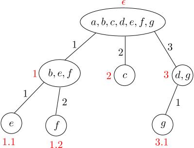
Figure 1: A history tree

Fact 1

The number of the nodes in each history tree of a non-deterministic Büchi automaton with $n$ states is no more than $n$.

Proof:

By the definition of history trees, the labels of siblings are disjoint (P2) and the label of each node contains at leat a state not appearing in any labels of its children (P3). That is any node $v$ in the history tree must have at least one state (in the Büchi automaton) which is specific to $v$ other than any nodes in the history tree. Consequently, the history tree can contain at most $n$ different nodes. ∎

Minor modification of history trees

History trees presented in this paper are different from the ones given in [15] where each node in a history tree is implicitly named as a sequence of non-negative integers. This small modification will not change the results presented in [15] but useful in reducing index complexity.

III-B Construction of History Trees

For a nondeterministic Büchi automaton $A=(\Sigma,Q,Q_{0},$ $\delta,\lambda)$, the initial history tree is $\langle T_{0},l_{0}\rangle=\langle\{\epsilon\},l_{0}(\epsilon)=Q_{0}\rangle$ that contains only one node $\epsilon$ that is labeled with the set of initial states $Q_{0}$. For a history tree $\langle T,l\rangle$, and an input letter $\sigma\in\Sigma$ of $A$, a new history tree, the $\sigma$-successor $\langle\widehat{T},\widehat{l}\rangle$ of $\langle T,l\rangle$, can be constructed in four steps:

Step 1

We first construct a labelled tree $\langle T^{\prime},l^{\prime}:T^{\prime}\rightarrow 2^{Q}\rangle$ such that

• $T^{\prime}=T\cup\{\tau^{\prime}\mid\tau^{\prime}=\tau\cdot(deg_{T}(\tau)+1)\mbox{ for any }\tau\in T\}$. That is, $T^{\prime}$ is formed by taken all nodes from $T$, and new nodes which are all node $\tau\in T$ appending with $deg_{T}(\tau)+1$.

• the label $l^{\prime}(\tau^{\prime})$ of an old node $\tau^{\prime}\in T$ is the set $\delta(l(\tau^{\prime}),\sigma)=\bigcup_{q\in l(\tau^{\prime})}\delta(q,\sigma)$ of $\sigma$-successors of the states in the label of $\tau^{\prime}$, and

• the label $l^{\prime}(\tau\cdot(deg_{T}(\tau)+1))$ of a new node $\tau\cdot(deg_{T}(\tau)+1)$ is the set of final states in $\sigma$-successors of the states in the label of $\tau$, i.e. $\delta(l(\tau),\sigma)\cap\lambda$.

Step 2

In this step, P2 is re-established. We construct the tree $\langle T^{\prime},l^{\prime\prime}:T^{\prime}\rightarrow 2^{Q}\rangle$, where $l^{\prime\prime}$ is inferred from $l^{\prime}$ by removing all states in the label of a node $\tau^{\prime}=\tau\cdot i$ and all its descendants if it appears in the label $l^{\prime}(\tau\cdot j)$ of an older sibling $(j<i)$.

Step 3

P1 and P3 are re-established in the third step. We construct the tree $\langle T^{\prime\prime},l^{\prime\prime}:T^{\prime\prime}\rightarrow 2^{Q}\rangle$ by (a) removing all descendants of nodes $\tau$ such that the label of $\tau$ is not a proper superset of the union of the labels of the children of $\tau$; and (b) removing all nodes $\tau$ with an empty label $l^{\prime\prime}(\tau)=\emptyset$. The stable nodes whose descendant have been deleted due to rule (a) are accepting nodes.

Step 4

The tree resulting from step 3 satisfies P1 - P3, but it might be not order-closed, i.e. there exist unstable nodes in the tree. We construct the $\sigma$-successor $\langle\widehat{T},\widehat{l}:T\rightarrow 2^{Q}\setminus\{\emptyset\}\rangle$ of $\langle T,l\rangle$ by “compressing” $T^{\prime\prime}$ to an order-closed tree, using the compression function $comp:T^{\prime\prime}\rightarrow\omega^{*}$ that maps the empty word $\epsilon$ to $\epsilon$, and $\tau\cdot i$ to $comp(\tau)\cdot j$, where $j=|\{k<i\mid\tau\cdot k\in T^{\prime\prime}\}|+1$ is the number of older siblings of $\tau\cdot i$ plus $1$. Note that the nodes that renamed during this step are exactly those which are unstable.

III-C Acceptance on Transitions

Based on the above constructing procedure, for a given NBW, an equivalent Deterministic Rabin Transition Automaton (DRTW) can be inductively established by:

• Build the initial history tree;

• for each history tree, by the four steps presented before, construct its $\sigma$-successor history $T_{i+1}$ for each $\sigma\in\Sigma$;

• performed (2) repeatedly until no new history trees can be created.

Now upon this underlying automata structure, deterministic Rabin transition automata are defined.

Definition 3

The deterministic Rabin transition automaton that equivalents to a given NBW $A$ is $RT=(\Sigma,Q_{RT},Q_{RT0},\delta_{RT},\lambda_{RT})$, where alphabet $\Sigma$ is the same as the one of $A$; $Q_{RT}$ is the set of history trees w.r.t $A$; $Q_{RT0}$ is the initial history tree; $\delta_{RT}$ is the history transition relation; and $\lambda_{RT}=((A_{\tau_{1}},R_{\tau_{1}}),\ldots,(A_{\tau_{k}},R_{\tau_{k}}))$, $k\geq 1$, is the acceptance condition. $\blacksquare$

In each Rabin pair $(A_{\tau},R_{\tau})$, $\tau$ ranges over implicit names of nodes (in a history tree). $A_{\tau}$ is the set of transitions where $\tau$ is accepting, and $R_{\tau}$ the set of transitions in which $\tau$ is unstable. For an input word $\alpha:\omega\rightarrow\Sigma$ we call the sequence $\Pi=\langle T_{0},l_{0}\rangle,\langle T_{1},l_{1}\rangle,\ldots$ of history trees that start with the initial history tree $\langle T_{0},l_{0}\rangle$ and where, for every $i\in\omega$, $\langle T_{i},l_{i}\rangle$ is followed by $\alpha(i)$-successor $\langle T_{i+1},l_{i+1}\rangle$, the history trace of $\alpha$. Let $\Pi$ be the history trace of a word $\alpha$ on the deterministic Rabin transition automaton. $\alpha$ is accepted by the automaton if, and only if, $\mathsf{Inf}(\Pi)\cap A_{\tau_{i}}\not=\emptyset$ and $\mathsf{Inf}(\Pi)\cap R_{\tau_{i}}=\emptyset$ for some $(A_{\tau_{i}},R_{\tau_{i}})\in\lambda_{RT}$, $1\leq i\leq k$.

With these notations, the following useful results are proved in [15].

Lemma 1

An $\omega$-word $\alpha$ is accepted by a nondeterministic Büchi automaton $A$ if, and only if, there is a node $\tau\in\mathbb{N}_{>0}^{*}$ such that $\tau$ is eventually always stable and always eventually accepting in the history trace of $\alpha$. $\blacksquare$

Let $RT$ be the deterministic Rabin transition automaton obtained from the given non-deterministic Büchi automaton $A$. The following corollary can easily be derived from Lemma 1.

Corollary 2

$L(RT)=L(A)$. $\blacksquare$

Eventually, the following main result for the determinization of NBWs in Rabin transition acceptance condition is claimed [15].

Theorem 3

For a given nondeterministic Büchi automaton with $n$ states, we can construct a deterministic Rabin transition automaton with $o((1.65n)^{n})$ states and $2^{n-1}$ accepting pairs that recognizes the language of $A$. $\blacksquare$

The state complexity $o((1.65n)^{n})$ is due to the result:

$$hist(n)\subset o((1.65n)^{n})$$

where $hist(n)$ is the number of history trees for a Büchi automaton with $n$ states; the index complexity is based on the number of (identifiable) nodes in the history trees [15]. Note that even though there are at most $n$ nodes in each history tree, there are a total of $2^{n-1}$ different nodes (identified by name) which may be involved in the history transitions of the Büchi automaton with $n$ states.

Due to the lower-bound result in [17], the state complexity for the construction of deterministic Rabin transition automaton is tight. However, whether the exponential index complexity can be improved is interesting.

In [15], by enriching history trees with information about which node of the resulting tree was accepting or unstable in the third step of the transition, ordinary deterministic Rabin automata can also be achieved.

Theorem 4

For a given nondeterministic Büchi automaton with $n$ states, we can construct a deterministic Rabin automaton with $o((2.66n)^{n})$ states and $2^{n-1}$ accepting pairs that recognizes the language $L(A)$ of $A$. $\blacksquare$

Further, by introducing the later introduction record as a record tailored for ordered trees, deterministic automata with Parity acceptance condition is constructed [15] which exactly resembles Piterman’s determinization with Parity acceptance condition [11].

Theorem 5

For a given nondeterministic Büchi automaton with $n$ states, we can construct a deterministic parity automaton with $O(n!^{2})$ states and $2n$ priorities that recognizes the language $L(A)$ of $A$. $\blacksquare$

Note that the original state complexity of Piterman’s construction is $2n^{n}n!$. By giving a better analysis, Liu and Wang, independently, achieved a similar result ($2n(n!)^{2}$ states and $2n$ priorities) for Piterman’s construction [14]. Further, it also have the transformation from NBW to DRW with $O(n!^{2})$ states and $n$ priorities. However, in state of the art for the upper bound complexity of the transformation from NBW to DRW, it is hard to say which one in ($o((2.66n)^{n})$, $2^{n-1}$) and ($O(n!^{2})$, $n$) is better. Note that the first element in the pair denotes the state complexity while the second one in the pair indicates the index complexity.

IV Ordered Trees with Identifiers

This section presents ordered trees with identifiers that are ordered trees with each node annotated by a unique identifier.

IV-A Height of Nodes in Ordered Trees

Given an ordered tree $T$, the height of a node $\tau=t_{1}t_{2}\ldots t_{n}\in T$ is $\mathit{height}(\tau):=\sum\limits_{i=1}^{len(\tau)}t_{i}$. For instance, the height of each node in the ordered tree in Fig.2 (1) is written inside the nodes as depicted in Fig.2 (2).

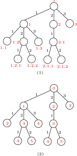
Figure 2: Height of nodes in ordered trees

With respect to height of nodes in ordered trees, order closedness for ordered trees is defined below.

Definition 4 (Order Closedness)

An ordered tree is order-closed if, and only if, it satisfies the following three conditions:

• C1: The height of the root node is $0$;

• C2: for each node with height being $n$, the height of its left sibling (older) is $n-1$ if it exists; and

• C3: for each node with height being $n$, the height of its leftmost child is $n+1$ if it exists. $\blacksquare$

If a node violates at least one of the above three conditions, it is an imbalanced node. Further, we call an imbalanced node, its younger siblings and their respective descendants unstable nodes; and the rest are stable nodes. (Thus, in particular, an imbalanced node is unstable.) Accordingly, we observe that whether a node in an ordered tree is imbalanced (respectively unstable and stable) depends on the height, which contains less information than implicit names, of nodes in the ordered trees. Note that if the ordered trees we use are exactly the same as Schewe’s [15], i.e. each integer in the name sequence is greater or equal to $0$, the above properties for ordered tree will not hold.

IV-B Partial Order Relation

We define a partial order relation $\preceq$ over nodes in a tree. Let $\tau=t_{1}t_{2}\cdot\cdot\cdot t_{n}$ and $\tau^{\prime}$ be nodes of an ordered tree $T$. We define $\tau^{\prime}\preceq\tau$ just if $\tau^{\prime}$ is a proper prefix $t_{0}t_{1}\ldots t_{m}$, $m<n$, of $\tau$ concatenated with $s$ where $s=\epsilon$ or $s\in\{1,\cdots,t_{m+1}-1\}$. The partial order relation $\preceq$ precisely characterizes the relationship (in stable or unstable situation) among nodes in an ordered tree. Suppose $\tau^{\prime}\preceq\tau$ for two different nodes in $T$. In case $\tau^{\prime}$ is unstable, $\tau$ is also unstable. Accordingly, w.r.t. each node $\tau$ in a tree $T$, a maximal chain $C(\tau)=\{\tau^{\prime}\mid\tau^{\prime}\in T,\mbox{ and }\tau^{\prime}\preceq\tau\}$ can be obtained. It is pointed out that for each node $\tau$ of an ordered tree, $height(\tau)=|C(\tau)|$. For instance, for $\tau_{5}$ in Fig. 3,

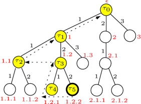
Figure 3: Partial order relation

a maximal chain $\tau_{0}\preceq\tau_{1}\preceq\tau_{2}\preceq\tau_{3}\preceq\tau_{4}\preceq\tau_{5}$ can be obtained. If $\tau_{i}$ is unstable for some $0\leq i\leq 4$, so is $\tau_{5}$; but if $\tau_{i}$ is stable for all $0\leq i\leq 4$ then $\tau_{5}$ is stable. Further, the number of the partial order chains in a tree depends on the number of the leaf nodes which is the right-most (youngest) child of its parent, e.g. nodes 1.1.2, 1.2.2, 1.3, 2.1.2, and 3 in Fig. 3.

IV-C $n$-Full Ordered Tree

We define $n$-full ordered tree which contains all the nodes that are possible to occur in an ordered tree with $n$ nodes (called $n$-ordered tree for convenience).

Definition 5 ($n$-Full Ordered Tree)

$n$-full ordered tree, $n\in\mathbb{N}_{{>}0}$, is an ordered tree where for each non-leaf node $\tau$ in the tree,

• the right-most child node $\tau^{\prime}$ of $\tau$ is a leaf node with $|C(\tau)|=n$;

• other children nodes of $\tau$ are non-leaf nodes. $\blacksquare$

The black part in Fig. 4 (1) - (6) shows $2$ to $7$-full ordered tree, respectively. Intuitively, $n$-full ordered tree, $n>1$, can be obtained from $(n-1)$-full ordered tree $T$ by adding a new right-most child node to each node in $T$.

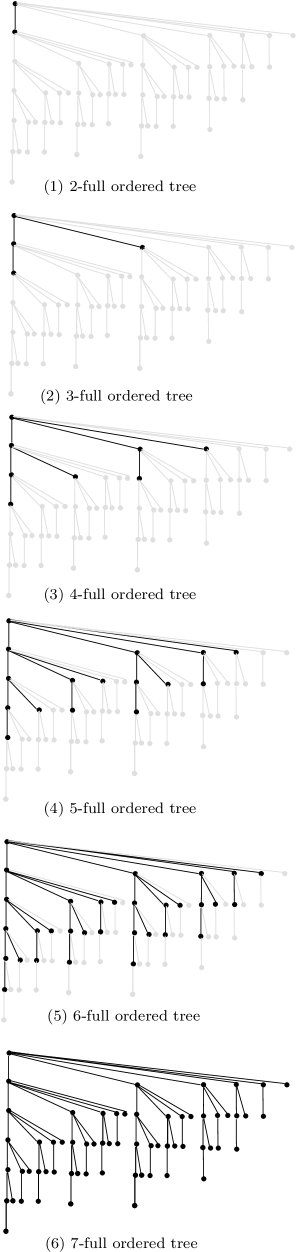
Figure 4: $n$-Full ordered tree

Fact 2

In $n$-full ordered tree, there are $2^{n-1}$ different nodes.

Proof:

The fact is obvious in case $n=1$ or $2$. Suppose the fact holds when $n=i$. That is there are totally $2^{i-1}$ nodes in $i$-full ordered tree $T$. Subsequently, $(i+1)$-full ordered tree $T^{\prime}$ can be obtained by creating a new right-most child for each node in $T$. Thus, there are $2^{i}$ nodes in $(i+1)$-full ordered tree. So the fact holds. ∎

Fact 2 shows that there are totally $2^{n-1}$ different nodes (identified by implicit names) possible to occur in an $n$-ordered tree. Thus, the index complexity of Schewe’s determinization is $2^{n-1}$ since implicit names of nodes in ordered trees containing $n$ nodes are utilized as the subscript when defining Rabin acceptance pairs. Fig. 5

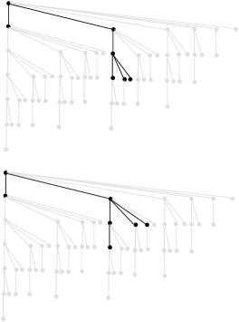
Figure 5: Ordered trees in full ordered tree

shows two different $7$-ordered trees (ordered trees with $7$ nodes) in the $7$-full ordered tree depicted in Fig. 4 (6).

Let $\tau$ and $\tau^{\prime}$ be two different nodes in an n-full ordered tree. $\tau$ and $\tau^{\prime}$ can occur in the same n-ordered tree if, and only if, $|C(\tau)\cup C(\tau^{\prime})|\leq n$. This indicates that if we assign a node $\tau$ of the $n$-full ordered tree a flag $f$ such that the flag is unique in ordered trees with no more that $n$ nodes where $\tau$ may occur, any other node $\tau^{\prime}$ where $|C(\tau)\cup C(\tau^{\prime\prime})|\leq n$ should be assigned a flag different to $f$. To use less flags meanwhile, a node $\tau^{\prime\prime}$ where $C(\tau)\cup C(\tau^{\prime\prime})>n$ can share the same flag with $\tau$. To further reduce the number of flags, we can use the height of each node as one property, and then for two nodes with different heights in an ordered tree, they can share the same flag. Accordingly, each node can be uniquely identified by its height in addition to flag in each ordered tree containing no more than $n$ nodes.

Lemma 6

At least $2^{\lceil(n-1)/2\rceil-1}$ different flags are required in $n$-full ordered tree such that each node in it can be uniquely identified in every $n$-ordered tree.

Proof:

Let $\tau$ be a node in an $n$-ordered tree with $height(\tau)=h$. There are $2^{h-1}$ different nodes with $height(\tau)=h$ in total that are possible to occur in an $n$-ordered tree where $\tau$ appears in case $h\leq\lceil(n-1)/2\rceil$; and $2^{n-h-1}$ otherwise. Thus, in case $h=\lceil(n-1)/2\rceil$, the maximal number of flags are required. Therefore, at least $2^{\lceil(n-1)/2\rceil-1}$ different flags are required in $n$-full ordered tree such that each node in any $n$-ordered tree is uniquely identified. ∎

IV-D $n$-Full Ordered Tree with Canonical Identifiers

Now we define $n$-full ordered tree with identifiers where every node in each $n$-ordered trees is annotated by a unique identifier.

Definition 6 ($n$-Full Ordered Tree with Identifiers)

$n$-full ordered tree with identifiers is a pair $\langle T,I\rangle$ where $T$ is $n$-full ordered tree, and $I:T\rightarrow(\mathbb{N},\mathbb{N}_{{>}0})$ maps each node $\tau$ in $T$ to its identifier $(h,f)$. Here $h$ is the height, $height(\tau)$, of $\tau$ and $f$ the flag of $\tau$, denoted by $flag(\tau)$, such that for any two different nodes, say $\tau$ and $\tau^{\prime}$, in $T$, $flag(\tau)\not=flag(\tau^{\prime})$ if $|C(\tau)\cup C(\tau^{\prime})|\leq n$ and $height(\tau)=height(\tau^{\prime})$. $\blacksquare$

There are different ways that are useful in assigning each node in $n$-full ordered tree a proper flag to obtain an $n$-full ordered tree with identifiers such that at most $2^{\lceil(n-1)/2\rceil-1}$ different flags are utilized. Here we present a canonical one $flag_{c}$ where each node is annotated by the minimal positive integer available in a predefined order.

Let $rm=\tau_{1}\ldots\tau_{x}$ be the sequence of the leaf nodes in $n$-full ordered tree in left-first order. For each $\tau_{i}$, $1\leq i\leq x$, in $rm$, a spine $sp_{i}$ is defined by $C(\tau_{i})\setminus(C(\tau_{1})\cup\ldots\cup C(\tau_{i-1}))$. Now we arrange all nodes in the tree as a sequence $se$ such that $\tau\leq\tau^{\prime}$ iff $\tau\preceq\tau^{\prime}$ or $\tau\in sp_{i}$, $\tau^{\prime}\in sp_{j}$, and $i\leq j$. We assign flags to the nodes in sequence $se$ from left to right. For the first $n$ nodes in $se$, we assign $1$ to $n$ to them in left-first order. In case the first $i$, $i>n$, nodes in $se$ have been assigned flags, for the $i+1^{th}$ node $\tau$ in the sequence, $flag_{c}(\tau)=Min(\{m\in\mathbb{N}_{{>}0}\mid\mbox{for any }\tau^{\prime}\mbox{ where }f(\tau^{\prime})=m\mbox{ and }height(\tau^{\prime})=height(\tau),\mbox{ it has }C(\tau^{\prime})\cup C(\tau)|>n\})$.

Definition 7

($n$-Full Ordered Tree with Canonical Identifiers) $n$-full ordered tree with canonical identifiers is a pair $\langle T,I_{c}\rangle$ where $T$ is $n$-full ordered tree, and $I:T\rightarrow(\mathbb{N},\mathbb{N}_{{>}0})$ maps each node $\tau$ in $T$ to its canonical identifier $(h,f_{c})$. Here $h$ is the height, $height(\tau)$, of $\tau$ and $f_{c}$ the canonical flag of $\tau$ obtained by $flag_{c}(\tau)$. $\blacksquare$

By the construction of $n$-Full Ordered Tree with Canonical Identifiers, the following fact is obtained.

Fact 3

That are at most $2^{\lceil(n-1)/2\rceil-1}$ different flags occurring in $n$-Full Ordered Tree with Canonical Identifiers.

Fig. 6 depicts $7$-full ordered tree with canonical identifers.

Figure 6: $7$-full ordered tree with canonical identifiers

We have developed a program to generate $n$-full ordered tree with canonical identifers automatically (http://web.xidian.edu.cn/ctian/files/20130417_183347.zip).

IV-E Ordered Trees with Canonical Identifiers

On $n$-full ordered tree with canonical identifiers, different n-ordered trees with canonical identifiers can be found. Let $T$ be one of the n-ordered trees with canonical identifiers. Each node in $T$ can be uniquely distinguished by its identifier. Accordingly, to reduce the index complexity of the determinization via history trees, in stead of the implicit names of nodes in ordered trees, we can identify each node in an ordered tree by its canonical identifer.

V Determinization of Büchi Automata via History Trees with Canonical Identifiers

This section presents the construction of deterministic Rabin transition automata via history trees with canonical identifiers from nondeterministic Büchi automata.

V-A History Trees with Canonical Identifiers

History trees with canonical Identifiers are built upon ordered trees with canonical identifiers.

Definition 8 (History Trees with Canonical Identifiers)

A history tree with canonical identifiers for a given nondeterministic Büchi automaton $B=(\Sigma,Q,Q_{0},\delta,\lambda)$ with $n$ states is a triple $\langle T,I_{c},l\rangle$ where $\langle T,I_{c}\rangle$ is an ordered tree with canonical identifiers, and $l:T\rightarrow 2^{Q}\setminus\{\emptyset\}$ labels each node of $T$ with a non-empty subset of $Q$, satisfying the following:

• The label of each node is non-empty.

• The labels of different children of a node are disjoint.

• The label of each node is a proper superset of the union of the labels of its children. $\blacksquare$

By Fact 1, there are at most $n$ nodes in the history trees with canonical identifiers for a given Büchi automaton with $n$ states. Fig. 7

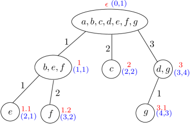
Figure 7: A history tree with canonical identifiers

shows a history tree with canonical identifiers where the label of a node is written inside the circle and the identifiers of nodes are in blue. It is a modification of the history tree (of a Büchi automaton with $7$ states) in Fig. 1 with each node annotated by an extra identifier adopt from 7-full ordered tree with canonical identifiers in Fig. 6.

V-B Construction of History Trees with Canonical Identifiers

Fix a nondeterministic Büchi automaton $B=(\Sigma,Q,Q_{0},$ $\delta,\lambda)$. The initial history tree with canonical identifiers $\langle T_{0},I_{c,0},l_{0}\rangle$ contains only one node $\epsilon$ with $I_{c,0}(\epsilon)=(0,1)$ and label being the set of initial states $Q_{0}$ of $B$.

Given a history tree with canonical identifiers $\langle T,I_{c},l\rangle$, and an input letter $\sigma\in\Sigma$ of Büchi automaton $B$, the $\sigma$-successor history tree with canonical identifiers $\langle\widehat{T},\widehat{I_{c}},\widehat{l}\rangle$ of $\langle T,I_{c},l\rangle$ is constructed in five steps below.

Step 1

We construct the a labeled tree with canonical identifiers $\langle T^{\prime},I_{c}^{\prime},l^{\prime}:T^{\prime}\rightarrow 2^{Q}\rangle$ such that

• $T^{\prime}=T\cup\{\tau^{\prime}=\tau\cdot(deg_{T}(\tau)+1)\mid\mbox{ for any }\tau\in T\}$. That is, $T^{\prime}$ is formed by taken all nodes from $T$ and creating the new child node $\tau\cdot(deg_{T}(\tau)+1)$ to any node $\tau\in T$;

• the label $l^{\prime}(\tau)=\delta(l(\tau),\sigma)$ of an old node $\tau\in T$ is the set $\delta(l(\tau),\sigma)=\bigcup_{q\in l(\tau)}\delta(q,\sigma)$ of $\sigma$-successors of the states in the label of $\tau$;

• the label $l^{\prime}(\tau^{\prime})=\delta(l(\tau),\sigma)\cap\lambda$ of a new node $\tau^{\prime}=\tau\cdot(deg_{T}(\tau)+1)$ is the set of final $\sigma$-successors of the states in the label of $\tau$;

• the identifiers of nodes are adopted from the n-full ordered tree with canonical identifiers. Here $n=|Q|$.

To illustrate the five steps of construction, we borrow the examples from [15] for ease of comparison with Schewe’s method. Fig. 8 shows all transitions for an input letter

Figure 8: Relevant fragment of a Büchi automaton

$\sigma$ from the states in the history tree with canonical identifiers in Fig. 7. The double circles indicate that the states $c$, $f$, and $g$ are final states.

Fig. 9 depicts the tree resulting from the history tree with canonical identifiers in Fig. 7 for the Büchi automaton and transition from Fig. 8 after Step 1 of the construction procedure. Each node of the tree from Fig. 7 has spawned a new child (marked by bold circle), whose label may be empty if, upon reading the input letter from any state in the label of the parent node, none of the new transition state is a final state. The canonical identifers of nodes are adopted from 7-full ordered tree with canonical identifers. The labels of nodes in gray will be deleted from the respective label in Step 2. Note that in Fig. 9, there may exist different nodes annotated with the same identifers, i.e. 1.3 and 4 are both annotated by $(4,4)$, since the tree resulted in this step may contain more than $n$ nodes (no more than $2n$ nodes in fact). However, at most one of the nodes with a same identifier will be kept in the eventually history tree with canonical identifers resulted in Step 5.

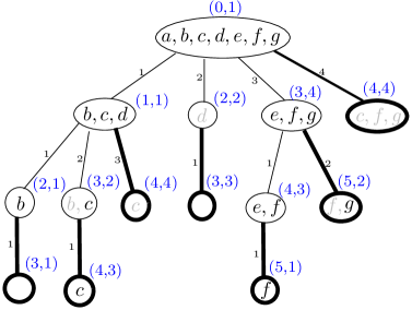
Figure 9: Step 1 of the construction procedure

Step 2

In this step, P2 is re-established. We construct the tree $\langle T^{\prime},I_{c}^{\prime},l^{\prime\prime}:T^{\prime}\rightarrow 2^{Q}\rangle$, where $l^{\prime\prime}$ is derived from $l^{\prime}$ by removing each state $q$ in the label of a node $\tau$ and all its descendants if $q$ appears in the label $l^{\prime}(\tau)$ of an older sibling.

Fig. 10 shows the tree that results from Step 2 of the construction procedure. In the resultant tree, the labels of the siblings are pairwise disjoint, but may be empty, and the union of the labels of the children of a node are not required to form a proper subset of their parent’s label. The part in dash lines will be deleted in Step 3.

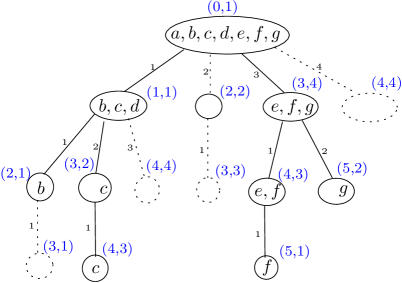
Figure 10: Step 2 of the construction procedure

Step 3

P1 is re-established in the third step. We construct the tree $\langle T^{\prime\prime},I_{c}^{\prime\prime},l^{\prime\prime}:T^{\prime\prime}\rightarrow 2^{Q}\rangle$ by removing all nodes $\tau$ with an empty label $l^{\prime\prime}(\tau)=\emptyset$.

The resulting tree is depicted in Fig. 11. The part in dash lines will be deleted in the next step.

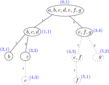
Figure 11: Step 3 of the construction procedure

Step 4

P3 is re-established in the this step. We construct the tree $\langle T^{\prime\prime\prime},I_{c}^{\prime\prime\prime},l^{\prime\prime\prime}:T^{\prime\prime\prime}\rightarrow 2^{Q}\rangle$ by removing all descendants of nodes $\tau$ if the label of $\tau$ is not a proper superset of the union of the labels of the children of $\tau$. The nodes whose descendant have been deleted because of this rule are called accepting nodes. For each accepting node, we add a symbol $\oplus$ on it to explicitly indicate that the node is accepting at the current step.

The resulting tree is depicted in Fig. 12 (1).

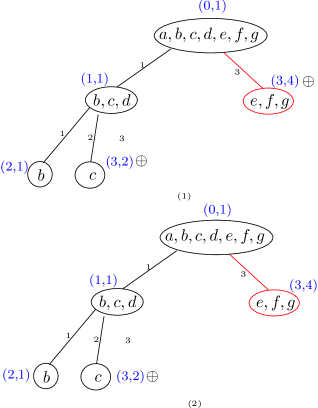
Figure 12: Step 4 of the construction procedure

The labels of the siblings are pairwise disjoint, and form a proper subset of their parent’s label, but the tree might not be order-closed. Two nodes with identifers being $(3,2)$ and $(3,4)$ are both accepting, as marked by $\oplus$. The nodes that will be renamed for establishing order closedness in Step 5 are drawn in red.

Step 5

The underling tree resulting from Step 4 satisfies properties P1-P3, but it may not be order-closed, i.e. there exist some imbalance nodes in the tree (e.g. $(3,4)$). We construct $\sigma$-successor $\langle\widehat{T},\widehat{I_{c}},\widehat{l}:T\rightarrow 2^{Q}\setminus\{\emptyset\}\rangle$ of $\langle T,I_{c},l\rangle$ by removing all the $\oplus$ symbols and “compressing” $T^{\prime\prime\prime}$ to an order-closed tree, using the compression function $comp:T^{\prime\prime\prime}\rightarrow\omega^{*}$ that maps the empty word $\epsilon$ to $\epsilon$, and $\tau\cdot i$ to $comp(\tau)\cdot j$, where $j=|\{k<i\mid\tau\cdot k\in T^{\prime\prime\prime}\}|+1$ is the number of older siblings of $\tau\cdot i$ plus $1$. Eventually, all the unstable nodes, i.e. imbalanced nodes as well as the descendants of the imbalanced nodes, and the younger siblings (and their descendants) of the imbalanced nodes, are renamed, and their identifiers are also updated. Further, for each node $\tau$ that is properly renamed in this step, we add a $\ominus$ symbol on the node before renaming (in the tree obtained in Step 4) to mean that this node is unstable in Step 5 if there is no $\oplus$ symbol on the node, otherwise we just remove the $\oplus$ symbol from the node.

Fig. 13 shows the $\sigma$-successor $\langle\widehat{T},\widehat{I_{c}},\widehat{l}:T\rightarrow 2^{Q}\setminus\{\emptyset\}\rangle$ of $\langle T,I_{c},l\rangle$ obtained in Step 5 and Fig. 7 (2) is the tree originally obtained in Step 4 but updated by Step 5.

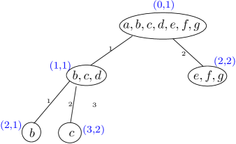
Figure 13: Step 5 of the construction procedure

Notice that the symbols $\oplus$ and $\ominus$ occur only in the trees created in the intermediate steps within the transitions, not in the history trees with canonical identifiers (states in the deterministic Rabin automata) eventually constructed.

V-C Deterministic Rabin Transition Automata

Based on the five-step construction procedure, for a given NBW, an equivalent deterministic Rabin transition automaton can be inductively constructed by:

• Build the initial history tree with canonical identifiers $(T_{0},I_{c,0},l_{0})$;

• for each history tree with canonical identifiers $(T_{i},I_{c,i},l_{i})$, by the five steps presented before, compute its $\sigma$-successor history tree with canonical identifiers $(T_{i+1},I_{c,i+1},l_{i+1})$ for each $\sigma\in\Sigma$.

• (2) is repeated until no new history trees with canonical identifiers can be created.

On this underlying automata structure, deterministic Rabin transition automata are defined.

Definition 9

The deterministic Rabin transition automaton equivalent to a given NBW $B$ is $RT=(\Sigma,Q_{RT},Q_{RT0},\delta_{RT},\lambda_{RT})$, where $Q_{RT}$ is the set of history trees with canonical identifiers w.r.t $B$; $Q_{RT0}$ the initial history trees with canonical identifiers; $\delta_{RT}$ the transition relation that is established during the construction of history trees with canonical identifiers; and $\lambda_{RT}=((A_{I1},R_{I1}),\ldots,(A_{Ii},R_{Ik}))$ the Rabin acceptance condition. $\blacksquare$

In each Rabin pair $(A_{I},R_{I})$, $I$ ranges over the canonical identifiers appearing in the history trees with canonical identifiers. $A_{I}$ is the set of transitions through which node $\tau$ with identifier being $I$ is accepting (annotated by $\oplus$), while $R_{I}$ is the set of transitions through which node $\tau$ with identifier being $I$ is unstable (annotated by $\ominus$).

For an input word $\alpha:\omega\rightarrow\Sigma$, we call the sequence $\Pi=\langle T_{0},I_{c,0},l_{0}\rangle,\langle T_{1},I_{c,1},l_{1}\rangle,\ldots$ of history trees with canonical identifiers that starts with the initial history trees with canonical identifiers $\langle T_{0},I_{c,0},l_{0}\rangle$ and where, for every $i\in\omega$, $\langle T_{i},I_{c,i},l_{i}\rangle$ is followed by $\alpha(i)$-successor $\langle T_{i+1},I_{c,i+1},l_{i+1}\rangle$, the history trace with canonical identifiers of $\alpha$. Let $\Pi$ be the history trace with canonical identifiers of a word $\alpha$ on the deterministic Rabin transition automaton. $\alpha$ is accepted by the automaton if, and only if, $\mathsf{Inf}(\Pi)\cap A_{Ii}\not=\emptyset$ and $\mathsf{Inf}(\Pi)\cap R_{Ii}=\emptyset$ for some $(A_{Ii},R_{Ii})$, $1\leq i\leq k$.

Let $RT$ be the deterministic Rabin transition automaton obtained from the given non-deterministic Büchi automaton $B$.

Theorem 7

$L(RT)=L(B)$.

Proof:

The theorem is proved by appealing to Lemma 1.
$\Rightarrow$: Given a history trace with canonical identifiers $\widehat{\Pi}$ such that $\mathsf{Inf}(\widehat{\Pi})\cap A_{Ii}\not=\emptyset$ and $\mathsf{Inf}(\widehat{\Pi})\cap R_{Ii}=\emptyset$, for some $i\geq 1$. By the construction of history trees with canonical identifiers, there exists some transition between two history trees with canonical identifiers (in $A_{Ii}$) containing node $\tau$ with $Ii$ being the identifier, such that $\tau$ is always eventually accepting since $\mathsf{Inf}(\widehat{\Pi})\cap A_{Ii}\not=\emptyset$. Further $\tau$ is eventually always stable because $\mathsf{Inf}(\widehat{\Pi})\cap R_{Ii}=\emptyset$ (in case $\tau$ is unstable in some transition in the loop, $\mathsf{Inf}(\widehat{\Pi})\cap R_{Ij}\not=\emptyset$).
$\Leftarrow$: Suppose history trace with canonical identifiers $\Pi$ contains node $\tau$, which is always eventually accepting and eventually always stable. By the construction of Rabin automata, there must exists $Ii$ which is the identifier of $\tau$ in the history trees with canonical identifiers such that $\mathsf{Inf}(\Pi)\cap A_{Ii}\not=\emptyset$ since $\tau$ is always eventually accepting (thus included in $A_{Ii}$). Further, $\mathsf{Inf}(\Pi)\cap R_{Ii}=\emptyset$ since $\tau$ is eventually always stable. ∎

Theorem 8

For a given nondeterministic Büchi automaton $B$ with $n$ states, we can construct a deterministic Rabin transition automaton with $o((1.65n)^{n})$ states and $2^{\lceil(n-1)/2\rceil}$ accepting pairs at most that recognizes the language $L(B)$ of $B$.

Proof:

For the state complexity, by the construction of history trees with canonical identifiers, for each node $\tau$ that is possible to occur in a history tree of a Büchi automaton with $n$ states, a unique identifier is assigned to the node and keeps unchanged no matter whether it occurs in a history tree. Thus, we cannot find two distinct history trees with canonical identifiers in the determinization construction of $B$ such that they coincide after the identifiers have been erased. So, $histf(n)=hist(n)\subset o((1.65n)^{n})$. Here $histf(n)$ is the number of history trees with canonical identifiers for a given nondeterministic Büchi automata with $n$ states.

Further, by Fact 3, for the nodes with height being $h$, at most $2^{h-1}$ different flags are required in case $h\leq\lceil(n-1)/2\rceil$; and $2^{n-h-1}$ otherwise. Thus, at most $2^{\lceil(n-1)/2\rceil}$ identifiers are required in $n$-full ordered tree. As a result, $2^{\lceil(n-1)/2\rceil}$ accepting pairs at most are required at most in the obtained deterministic Rabin transition automata. ∎

By the lower bound result of the state complexity in [17], the state complexity of the new construction is optimal. Further, by Lemma 6, the index complexity is already tight. Thus, we have the following corollary.

Corollary 9

Construction of deterministic Rabin transition automata from nondeterministic Büchi automata via history trees with canonical identifiers is optimal.

VI From Nondeterministic Büchi Automata to Ordinary Rabin Automata

By moving the acceptance and unstable information, i.e. $\oplus$ and $\ominus$ symbols, from transitions to states (history trees with canonical identifiers), a deterministic Rabin transition automaton can be equivalently transformed as an ordinary deterministic Rabin automaton. For convenience, we call history trees with canonical identifiers decorated with acceptance and unstable information enriched history trees with canonical identifiers.

Let $ehistf(n)$ be the number of enriched history trees with canonical identifiers for a given nondeterministic Büchi automata with $n$ states. The following lemma can be obtained.

Lemma 10

For a given nondeterministic Büchi automaton $B$ with $n$ states, we have $ehistf(n)\subset o((2.66n)^{n})$.

Proof:

Enriched history trees with canonical identifiers possible occurring in determinization construction are actually ordered trees decorated with (1) labels, (2) canonical identifiers, and (3) accepting and unstable information. It can be easily observed that ordered trees decorated with (1) labels and (3) accepting and unstable information, called enriched history trees are exactly the enriched history trees in [15] used by Schewe for defining the ordinary Rabin acceptance condition. By Theorem 4, $ehist(n)\subset o((2.66n)^{n})$. Here $ehist(n)$ denotes the number of the enriched history trees for an NBW with $n$ states. Further, $ehistf(n)=ehist(n)\subset o((2.66n)^{n})$ since additional identifiers will not increase the number of trees. ∎

Theorem 11

For a given nondeterministic Büchi automaton $B$ with $n$ states, we can construct a deterministic Rabin automaton with $o((2.66n)^{n})$ states and at most $2^{\lceil(n-1)/2\rceil}$ accepting pairs that recognizes the language $L(B)$ of $B$.

Proof:

The state complexity has been obtained in Lemma 10 and the index complexity can be proved similar to Theorem 8. ∎

VII Conclusion

In this paper, we present a transformation from Büchi automata of size $n$ into deterministic Rabin transition automata with $o((1.65n)^{n})$ states and $2^{\lceil(n-1)/2\rceil}$ Rabin pairs. This improves the current best construction with the same (and optimal) state complexity, but $2^{n-1}$ Rabin pairs. We also present a construction of ordinary deterministic Rabin automata from NBWs with $o((2.66n)^{n})$ states and $2^{\lceil(n-1)/2\rceil}$ accepting pairs.

References

- [1] M. Clark, O. Gremberg and A. Peled. Model Checking. The MIT Press, 2000.
- [2] J-P. Katoen. Concepts, Algorithms and Tools for Model Checking. Arbeitsberichte der Informatik, Friedrich-Alexander-Universitaet Erlangen-Nuernberg, Vol. 32, No. 1, 1999.
- [3] J. R. Büchi. On a decision method in restricted second order arithmetic. In Proceedings of the International Congress on Logic, Method, and Philosophy of Science, pages 1-12. Stanford University Press, 1962.
- [4] W. Thomas. Languages, automata and logic. In Handbook of Formal Languages, volume 3, pages 389-455. Springer-Verlag, Berlin, 1997.
- [5] Udi Boker, Orna Kupferman: Co-ing Büchi Made Tight and Useful. LICS 2009: 245-254.
- [6] Udi Boker, Orna Kupferman: The Quest for a Tight Translation of Büchi to co-Büchi Automata. Fields of Logic and Computation 2010: 147-164.
- [7] Udi Boker, Orna Kupferman: Co-Büching Them All. FOSSACS 2011: 184-198.
- [8] Rabin, M.O., Scott, D.S.: Finite automata and their decision problems. IBM Journal of Research and Development 3, 115-125 (1959)
- [9] Safra, S.: On the complexity of omega-automata. In: FOCS 1988: 319-327.
- [10] Muller, D.E., Schupp, P.E.: Simulating alternating tree automata by nondeterministic automata: new results and new proofs of the theorems of Rabin, McNaughton and Safra. Theoretical Computer Science 141, 69-107 (1995)
- [11] Piterman, N.: From nondeterministic Büuchi and Streett automata to deterministic parity automata. Journal of Logical Methods in Computer Science 3 (2007)
- [12] Muller, D.E.: Infinite sequences and finite machines. In: Proceedings of the 4th Annual Symposium on Switching Circuit Theory and Logical Design (FOCS 1963), pp. 3-16. IEEE Computer Society Press (1963)
- [13] McNaughton, R.: Testing and generating infinite sequences by a finite automaton. Information and Control 9, 521-530 (1966)
- [14] Wanwei Liu, Ji Wang: A tighter analysis of Piterman’s Büchi determinization. Inf. Process. Lett. 109(16): 941-945 (2009)
- [15] Sven Schewe: Tighter Bounds for the Determinisation of Büchi Automata. FOSSACS 2009: 167-181
- [16] M. Michel. Complementation is more difficult with automata on infinite words. CNET, Paris, 1988.
- [17] Thomas Colcombet, Konrad Zdanowski: A Tight Lower Bound for Determinization of Transition Labeled Büchi Automata. ICALP (2) 2009: 151-162
- [18] Qiqi Yan. Lower bounds for complementation of omega-automata via the full automata technique. ICALP 2006: 589-600.