Orthogonal Rank-One Matrix Pursuit
for Low Rank Matrix Completion

Zheng Wang School of Computing, Informatics, and Decision Systems Engineering, Arizona State University, Tempe, Arizona 85287, USA (zhengwang@asu.edu, jieping.ye@asu.edu).    Ming-Jun Lai Department of Mathematics, The University of Georgia, Athens, GA 30602, USA (mjlai@math.uga.edu).    Zhaosong Lu Department of Mathematics, Simon Frasor University, Burnaby, BC, V5A 156, Canada (zhaosong@sfu.ca).    Wei Fan Huawei Noah’s Ark Lab Hong Kong (wei.fan@gmail.com).    Hasan Davulcu11footnotemark: 1    Jieping Ye11footnotemark: 1
Abstract

In this paper, we propose an efficient and scalable low rank matrix completion algorithm. The key idea is to extend orthogonal matching pursuit method from the vector case to the matrix case. We further propose an economic version of our algorithm by introducing a novel weight updating rule to reduce the time and storage complexity. Both versions are computationally inexpensive for each matrix pursuit iteration, and find satisfactory results in a few iterations. Another advantage of our proposed algorithm is that it has only one tunable parameter, which is the rank. It is easy to understand and to use by the user. This becomes especially important in large-scale learning problems. In addition, we rigorously show that both versions achieve a linear convergence rate, which is significantly better than the previous known results. We also empirically compare the proposed algorithms with several state-of-the-art matrix completion algorithms on many real-world datasets, including the large-scale recommendation dataset Netflix as well as the MovieLens datasets. Numerical results show that our proposed algorithm is more efficient than competing algorithms while achieving similar or better prediction performance.

keywords:
Low rank, singular value decomposition, rank minimization, matrix completion, matching pursuit

1 Introduction

Recently, low rank matrix learning has attracted significant attentions in machine learning and data mining due to its wide range of applications, such as collaborative filtering, dimensionality reduction, compressed sensing, multi-class learning and multi-task learning. See [1, 2, 3, 7, 9, 23, 34, 40, 37] and the references therein. In this paper, we consider the general form of low rank matrix completion: given a partially observed real-valued matrix 𝐘n×m𝐘superscript𝑛𝑚{\bf Y}\in\Re^{n\times m}, the low rank matrix completion problem is to find a matrix 𝐗n×m𝐗superscript𝑛𝑚{\bf X}\in\Re^{n\times m} with minimum rank that best approximates the matrix 𝐘𝐘{\bf Y} on the observed elements. The mathematical formulation is given by

min𝐗n×mrank(𝐗)s.t.PΩ(𝐗)=PΩ(𝐘),subscript𝐗superscript𝑛𝑚𝑟𝑎𝑛𝑘𝐗formulae-sequence𝑠𝑡subscript𝑃Ω𝐗subscript𝑃Ω𝐘\begin{array}[]{cl}\min\limits_{{\bf X}\in\Re^{n\times m}}&rank({\bf X})\\ s.t.&P_{\Omega}({\bf X})=P_{\Omega}({\bf Y}),\end{array} (1)

where ΩΩ\Omega is the set of all index pairs (i,j)𝑖𝑗(i,j) of observed entries, and PΩsubscript𝑃ΩP_{\Omega} is the orthogonal projector onto the span of matrices vanishing outside of ΩΩ\Omega.

1.1 Related Works

As it is intractable to minimize the matrix rank exactly in the general case, many approximate solutions have been proposed to attack the problem (1) (cf., e.g. [7, 24, 28]). A widely used convex relaxation of matrix rank is the trace norm or nuclear norm [7]. The matrix trace norm is defined by the Schatten p𝑝p-norm with p=1𝑝1p=1. For matrix 𝐗𝐗{\bf X} with rank r𝑟r, its Schatten p𝑝p-norm is defined by (i=1rσip)1/psuperscriptsubscriptsuperscript𝑟𝑖1subscriptsuperscript𝜎𝑝𝑖1𝑝(\sum^{r}_{i=1}\sigma^{p}_{i})^{1/p}, where {σi}subscript𝜎𝑖\{\sigma_{i}\} are the singular values of 𝐗𝐗{\bf X} and without loss of generality we assume they are sorted in descending order. Thus, the trace norm of 𝐗𝐗{\bf X} is the 1subscript1\ell_{1} norm of the matrix spectrum as 𝐗=i=1r|σi|subscriptnorm𝐗subscriptsuperscript𝑟𝑖1subscript𝜎𝑖||{\bf X}||_{*}=\sum^{r}_{i=1}|\sigma_{i}|. Then the convex relaxation for problem (1) is given by

min𝐗n×m𝐗s.t.PΩ(𝐗)=PΩ(𝐘).subscript𝐗superscript𝑛𝑚subscriptnorm𝐗formulae-sequence𝑠𝑡subscript𝑃Ω𝐗subscript𝑃Ω𝐘\begin{array}[]{cl}\min\limits_{{\bf X}\in\mathcal{R}^{n\times m}}&||{\bf X}||_{*}\\ s.t.&P_{\Omega}({\bf X})=P_{\Omega}({\bf Y}).\end{array} (2)

Cai et al. [6] propose an algorithm based on soft singular value thresholding (SVT). Keshavan et al. [21] and Meka et al. [18] develop more efficient algorithms by using the top-k𝑘k singular pairs.

Many other algorithms have been developed to solve the trace norm penalized problem:

min𝐗n×mPΩ(𝐗)PΩ(𝐘)F2+λ𝐗.subscript𝐗superscript𝑛𝑚subscriptsuperscriptnormsubscript𝑃Ω𝐗subscript𝑃Ω𝐘2𝐹𝜆subscriptnorm𝐗\min_{{\bf X}\in\mathcal{R}^{n\times m}}||P_{\Omega}({\bf X})-P_{\Omega}({\bf Y})||^{2}_{F}+\lambda||{\bf X}||_{*}. (3)

Ji et al. [20], Liu et al. [27] and Toh et al. [44] independently propose to employ the proximal gradient algorithm to improve the algorithm of [6] by significantly reducing the number of iterations. They obtain an ϵitalic-ϵ\epsilon-accurate solution in O(1/ϵ)𝑂1italic-ϵO(1/\sqrt{\epsilon}) steps. More efficient soft singular vector thresholding algorithms are proposed in [29, 30] by investigating the factorization property of the estimated matrix. Each step of the algorithms requires the computation of a partial SVD for a dense matrix. In addition, several methods approximate the trace norm using its variational characterizations [32, 40, 46, 37], and proceed by alternating optimization. However these methods lack global convergence guarantees.

Solving these low rank or trace norm problems is computationally expensive for large matrices, as it involves computing singular value decomposition (SVD). Most of the methods above involve the computation of SVD or truncated SVD iteratively, which is not scalable to large-scale problems. How to solve these problems efficiently and accurately for large-scale problems attracts much attention in recent years.

Recently, the coordinate gradient descent method has been demonstrated to be efficient in solving sparse learning problems in the vector case [11, 39, 47, 48]. The key idea is to solve a very simple one-dimensional problem (for one coordinate) in each iteration. One natural question is whether and how such method can be applied to solve the matrix completion problem. Some progress has been made recently along this direction. Dudík et al. [9] propose a coordinate gradient descent solution for the trace norm penalized problem. They recast the non-smooth objective in problem (3) as a smooth one in an infinite dimensional rank-one matrix space, then apply the coordinate gradient algorithm on the collection of rank-one matrices. Zhang et al. [49] further improve the efficiency using the boosting method, and the improved algorithm guarantees an ϵitalic-ϵ\epsilon-accuracy within O(1/ϵ)𝑂1italic-ϵO(1/{\epsilon}) iterations. Although these algorithms need slightly more iterations than the proximal methods, they are more scalable as they only need to compute the top singular vector pair in each iteration. Note that the top singular vector pair can be computed efficiently by the power method or Lanczos iterations [13]. Jaggi et al. [17] propose an algorithm which achieves the same iteration complexity as the algorithm in [49] by directly applying the Hazan’s algorithm [15]. Tewari et al. [42] solve a more general problem based on a greedy algorithm. Shalev-Shwartz et al. [38] further reduce the number of iterations based on a heuristic without theoretical guarantees.

Most methods based on the top singular vector pair include two main steps in each iteration. The first step involves computing the top singular vector pair, and the second step refines the weights of the rank-one matrices formed by all top singular vector pairs obtained up to the current iteration. The main differences among these algorithms lie in how they refine the weights. The Jaggi’s algorithm (JS) [17] directly applies the Hazan’s algorithm [15], which relied on the Frank-Wolfe algorithm [10]. It updates the weights with a small step size and does not consider further refinement. It does not use all information in each step, which leads to a slow convergence rate. Similar to JS, Tewari et al. [42] use a small update step size for a general structure constrained problem. The greedy efficient component optimization (GECO) [38] optimizes the weights by solving another time consuming optimization problem. It involves a smaller number of iterations than the JS algorithm. However, the sophisticated weight refinement leads to a higher total computational cost. The lifted coordinate gradient descent algorithm (Lifted) [9] updates the rank-one matrix basis with a constant weight in each iteration, and conducts a LASSO type algorithm [43] to fully correct the weights. The weights for the basis update are difficult to tune: a large value leads to divergence; a small value makes the algorithm slow [49]. The matrix norm boosting approach (Boost) [49] learns the update weights and designs a local refinement step by a non-convex optimization problem which is solved by alternating optimization. It has a sub-linear convergence rate.

Let us summarize their common drawbacks as follows:

  • The weight refinement steps are inefficient, resulting in a slow convergence rate. The current best convergence rate is O(1/ϵ)𝑂1italic-ϵO(1/{\epsilon}). Some refinement steps themselves contain computationally expensive iterations [9, 49], which do not scale to large-scale data.

  • They have heuristic-based tunable parameters which are not easy to use. However, these parameters severely affect their convergence speed and the approximation result. In some algorithms, an improper parameter even makes the algorithm diverge [6, 9].

In this paper, we present a simple and efficient algorithm to solve the low rank matrix completion problem. The key idea is to extend the orthogonal matching pursuit (OMP) procedure [35] from the vector case to the matrix case. In each iteration, a rank-one basis matrix is generated by the left and right top singular vectors of the current approximation residual. In the standard version of the proposed algorithm, we fully update the weights for all rank-one matrices in the current basis set at the end of each iteration by performing an orthogonal projection of the observation matrix onto their spanning subspace. The most time-consuming step of the proposed algorithm is to calculate the top singular vector pair of a sparse matrix, which costs O(|Ω|)𝑂ΩO(|\Omega|) operations in each iteration. An appealing feature of the proposed algorithm is that it has a linear convergence rate. This is quite different from traditional orthogonal matching pursuit or weak orthogonal greedy algorithms, whose convergence rate for sparse vector recovery is sub-linear as shown in [26]. See also [8], [41], [45] for an extensive study on various greedy algorithms. With this rate of convergence, we only need O(log(1/ϵ))𝑂1italic-ϵO(\log(1/\epsilon)) iterations for achieving an ϵitalic-ϵ\epsilon-accuracy solution.

One drawback of the standard algorithm is that it needs to store all rank-one matrices in the current basis set for full weight updating, which contains r|Ω|𝑟Ωr|\Omega| elements in the r𝑟r-th iteration. This makes the storage complexity of the algorithm dependent on the number of iterations, which restricts the approximation rank especially for large-scale matrices. To tackle this problem, we propose an economic weight updating rule for this algorithm. In this economic version of the proposed algorithm, we only track two matrices in each iteration. One is the current estimated matrix and the other one is the pursued rank-one matrix. When restricted to the observations in ΩΩ\Omega, each has |Ω|Ω|\Omega| nonzero elements. Thus the storage requirement, i.e., 2|Ω|2Ω2|\Omega|, keeps the same in different iterations, which is the same as the greedy algorithms [17, 42]. Interestingly, we show that using this economic updating rule we still retain the linear convergence rate. To the best of our knowledge, our proposed algorithms are the fastest among all related methods in the literature. We verify the efficiency of our algorithms empirically on large-scale matrix completion problems, such as MovieLens [31] and Netflix [4, 5], see §7.

The main contributions of our paper are:

  • We propose a computationally efficient and scalable algorithm for matrix completion, which extends the orthogonal matching pursuit from the vector case to the matrix case.

  • We theoretically prove the linear convergence rate of our algorithm. As a result, we only need O(log(1/ϵ))𝑂1italic-ϵO(\log(1/{\epsilon})) steps to obtain an ϵitalic-ϵ\epsilon-accuracy solution, and in each step we only need to compute the top singular vector pair, which can be computed efficiently.

  • We further reduce the storage complexity of our algorithm based on an economic weight updating rule while retaining the linear convergence rate. This version of our algorithm has a constant storage complexity which is independent of the approximation rank and is more practical for large-scale matrices.

  • Both versions of our algorithm have only one free parameter, i.e., the rank of the estimated matrix. The proposed algorithm is guaranteed to converge, i.e., no risk of divergence.

1.2 Notations and Organization

Let 𝐘=(𝐲1,,𝐲m)n×m𝐘subscript𝐲1subscript𝐲𝑚superscript𝑛𝑚{\bf Y}=({\bf y}_{1},\cdots,{\bf y}_{m})\in\Re^{n\times m} be an n×m𝑛𝑚n\times m real matrix, and Ω{1,,n}×{1,,m}Ω1𝑛1𝑚\Omega\subset\{1,\cdots,n\}\times\{1,\cdots,m\} denote the indices of the observed entries of 𝐘𝐘{\bf Y}. PΩsubscript𝑃ΩP_{\Omega} is the projection operator onto the space spanned by the matrices vanishing outside of ΩΩ\Omega so that the (i,j)𝑖𝑗(i,j)-th component of PΩ(𝐘)subscript𝑃Ω𝐘P_{\Omega}({\bf Y}) equals to 𝐘i,jsubscript𝐘𝑖𝑗{\bf Y}_{i,j} for (i,j)Ω𝑖𝑗Ω(i,j)\in\Omega and zero otherwise. The Frobenius norm of 𝐘𝐘{\bf Y} is defined as 𝐘F=i,j𝐘i,j2subscriptnorm𝐘𝐹subscript𝑖𝑗subscriptsuperscript𝐘2𝑖𝑗||{\bf Y}||_{F}=\sqrt{\sum_{i,j}{\bf Y}^{2}_{i,j}}. Let vec(𝐘)=(𝐲1T,,𝐲mT)T𝑣𝑒𝑐𝐘superscriptsubscriptsuperscript𝐲𝑇1subscriptsuperscript𝐲𝑇𝑚𝑇vec({\bf Y})=({\bf y}^{T}_{1},\cdots,{\bf y}^{T}_{m})^{T} denote a vector reshaped from matrix 𝐘𝐘{\bf Y} by concatenating all its column vectors. Let 𝐲˙˙𝐲\dot{\bf y} be the vector by concatenating all observed entries in 𝐘𝐘{\bf Y}, which is composed by keeping the observed elements in the vector vec(PΩ(𝐘))𝑣𝑒𝑐subscript𝑃Ω𝐘vec(P_{\Omega}({\bf Y})). The Frobenius inner product of two matrices 𝐗𝐗{\bf X} and 𝐘𝐘{\bf Y} is defined as 𝐗,𝐘=trace(𝐗T𝐘)𝐗𝐘𝑡𝑟𝑎𝑐𝑒superscript𝐗𝑇𝐘\langle{\bf X},{\bf Y}\rangle=trace({\bf X}^{T}{\bf Y}), which also equals to the component-wise inner product of the corresponding vectors as vec(𝐗),vec(𝐘)𝑣𝑒𝑐𝐗𝑣𝑒𝑐𝐘\langle vec({\bf X}),vec({\bf Y})\rangle. Given a matrix 𝐀n×m𝐀superscript𝑛𝑚{\bf A}\in\Re^{n\times m}, we denote PΩ(𝐀)subscript𝑃Ω𝐀P_{\Omega}(\bf A) by 𝐀Ωsubscript𝐀Ω{\bf A}_{\Omega}. For any two matrices 𝐀,𝐁n×m𝐀𝐁superscript𝑛𝑚{\bf A},{\bf B}\in\Re^{n\times m}, we define

𝐀,𝐁Ω=𝐀Ω,𝐁Ω,subscript𝐀𝐁Ωsubscript𝐀Ωsubscript𝐁Ω\langle{\bf A},{\bf B}\rangle_{\Omega}=\langle{\bf A}_{\Omega},{\bf B}_{\Omega}\rangle,

𝐀Ω=𝐀,𝐀Ωsubscriptnorm𝐀Ωsubscript𝐀𝐀Ω\|{\bf A}\|_{\Omega}=\sqrt{\langle{\bf A},{\bf A}\rangle_{\Omega}}. Without further declaration, the matrix norm refers to the Frobenius norm, which could also be written as 𝐀=𝐀,𝐀norm𝐀𝐀𝐀\|{\bf A}\|=\sqrt{\langle{\bf A},{\bf A}\rangle}.

The rest of the paper is organized as follows: we present our algorithm in Section 2; Section 3 analyzes the convergence rate of the standard version of our algorithm; we further propose an economic version of our algorithm and prove its linear convergence rate in Section 4; Section 5 extends the proposed algorithm to a more general matrix sensing case, and presents its guarantee of finding the optimal solution under rank-restricted-isometry-property condition; in Section 6 we analyze the stability of both versions of our algorithms; empirical evaluations are presented in Section 7 to verify the efficiency and effectiveness of our algorithms. We finally conclude our paper in Section 8.

2 Orthogonal Rank-One Matrix Pursuit

It is well-known that any matrix 𝐗n×m𝐗superscript𝑛𝑚{\bf X}\in\Re^{n\times m} can be written as a linear combination of rank-one matrices, that is,

𝐗=𝐌(𝜽)=iθi𝐌i,𝐗𝐌𝜽subscript𝑖subscript𝜃𝑖subscript𝐌𝑖{\bf X}={\bf M}({\bm{\theta}})=\sum_{i\in\mathcal{I}}{\theta}_{i}{\bf M}_{i}, (4)

where {𝐌i:iI}conditional-setsubscript𝐌𝑖𝑖𝐼\{{\bf M}_{i}:i\in I\} is the set of all n×m𝑛𝑚n\times m rank-one matrices with unit Frobenius norm. Clearly, there is an infinitely many choice of 𝐌isubscript𝐌𝑖{\bf M}_{i}’s. Such a representation can be obtained via the standard SVD decomposition of 𝐗𝐗{\bf X}.

The original low rank matrix approximation problem aims to minimize the zero-norm of θ𝜃\theta subject to the constraint:

min𝜽𝜽0s.t.PΩ(𝐌(𝜽))=PΩ(𝐘),subscript𝜽subscriptnorm𝜽0formulae-sequence𝑠𝑡subscript𝑃Ω𝐌𝜽subscript𝑃Ω𝐘\begin{array}[]{ll}\min\limits_{\bm{\theta}}&||{\bm{\theta}}||_{0}\\[6.0pt] s.t.&P_{\Omega}({\bf M}({\bm{\theta}}))=P_{\Omega}({\bf Y}),\end{array} (5)

where 𝜽0subscriptnorm𝜽0||{\bm{\theta}}||_{0} denotes the number of nonzero elements of vector 𝜽𝜽{\bm{\theta}}.

If we reformulate the problem as

min𝜽PΩ(𝐌(𝜽))PΩ(𝐘)F2s.t.𝜽0r,subscript𝜽subscriptsuperscriptnormsubscript𝑃Ω𝐌𝜽subscript𝑃Ω𝐘2𝐹formulae-sequence𝑠𝑡subscriptnorm𝜽0𝑟\begin{array}[]{ll}\min\limits_{\bm{\theta}}&||P_{\Omega}({\bf M}({\bm{\theta}}))-P_{\Omega}({\bf Y})||^{2}_{F}\\[6.0pt] s.t.&||{\bm{\theta}}||_{0}\leq r,\end{array} (6)

we could solve it by an orthogonal matching pursuit type algorithm using rank-one matrices as the basis. In particular, we are to find a suitable subset with over-complete rank-one matrix coordinates, and learn the weight for each coordinate. This is achieved by executing two steps alternatively: one is to pursue the basis, and the other one is to learn the weights of the basis.

Suppose that after the (k(k-1)1)-th iteration, the rank-one basis matrices 𝐌1,,𝐌k1subscript𝐌1subscript𝐌𝑘1{\bf M}_{1},\ldots,{\bf M}_{k-1} and their current weight 𝜽k1superscript𝜽𝑘1{\bm{\theta}}^{k-1} are already computed. In the k𝑘k-th iteration, we are to pursue a new rank-one basis matrix 𝐌ksubscript𝐌𝑘{\bf M}_{k} with unit Frobenius norm, which is mostly correlated with the current observed regression residual 𝐑𝐤=PΩ(𝐘)𝐗k1subscript𝐑𝐤subscript𝑃Ω𝐘subscript𝐗𝑘1{\bf R_{k}}=P_{\Omega}({\bf Y})-{\bf X}_{k-1}, where

𝐗k1=(𝐌(𝜽k1))Ω=i=1k1θik1(𝐌i)Ω.subscript𝐗𝑘1subscript𝐌superscript𝜽𝑘1Ωsubscriptsuperscript𝑘1𝑖1subscriptsuperscript𝜃𝑘1𝑖subscriptsubscript𝐌𝑖Ω{\bf X}_{k-1}\ =\ ({\bf M}({\bm{\theta}}^{k-1}))_{\Omega}\ =\ \sum^{k-1}_{i=1}{\theta}^{k-1}_{i}({\bf M}_{i})_{\Omega}.

Therefore, 𝐌ksubscript𝐌𝑘{\bf M}_{k} can be chosen to be an optimal solution of the following problem:

max𝐌{𝐌,𝐑k:rank(𝐌)=1,𝐌F=1}.subscript𝐌:𝐌subscript𝐑𝑘formulae-sequencerank𝐌1subscriptnorm𝐌𝐹1\max_{\bf M}\{\langle{\bf M},{\bf R}_{k}\rangle:\ {\mathop{\operator@font rank}\nolimits({\bf M})=1,\ \|{\bf M}\|_{F}=1}\}. (7)

Notice that each rank-one matrix 𝐌𝐌{\bf M} with unit Frobenius norm can be written as the product of two unit vectors, namely, 𝐌=𝐮𝐯T𝐌superscript𝐮𝐯𝑇{\bf M}={\bf u}{\bf v}^{T} for some 𝐮n𝐮superscript𝑛{\bf u}\in\Re^{n} and 𝐯m𝐯superscript𝑚{\bf v}\in\Re^{m} with 𝐮=𝐯=𝟏norm𝐮norm𝐯1\|\bf u\|=\|\bf v\|=1. We then see that problem (7) can be equivalently reformulated as

max𝐮,𝐯{𝐮T𝐑k𝐯:𝐮=𝐯=𝟏}.subscript𝐮𝐯:superscript𝐮𝑇subscript𝐑𝑘𝐯norm𝐮norm𝐯1\max\limits_{{\bf u},{\bf v}}\{{\bf u}^{T}{\bf R}_{k}{\bf v}:\ \|\bf u\|=\|\bf v\|=1\}. (8)

Clearly, the optimal solution (𝐮,𝐯)subscript𝐮subscript𝐯({\bf u}_{*},{\bf v}_{*}) of problem (8) is a pair of top left and right singular vectors of 𝐑ksubscript𝐑𝑘{\bf R}_{k}. It can be efficiently computed by the power method [17, 9]. The new rank-one basis matrix 𝐌ksubscript𝐌𝑘{\bf M}_{k} is then readily available by setting 𝐌k=𝐮𝐯Tsubscript𝐌𝑘subscript𝐮superscriptsubscript𝐯𝑇{\bf M}_{k}={\bf u}_{*}{\bf v}_{*}^{T}.

After finding the new rank-one basis matrix 𝐌ksubscript𝐌𝑘{\bf M}_{k}, we update the weights 𝜽ksuperscript𝜽𝑘{\bm{\theta}}^{k} for all currently available basis matrices {𝐌1,,𝐌k}subscript𝐌1subscript𝐌𝑘\{{\bf M}_{1},\cdots,{\bf M}_{k}\} by solving the following least squares regression problem:

min𝜽ki=1kθi𝐌i𝐘Ω2.subscript𝜽superscript𝑘subscriptsuperscriptnormsubscriptsuperscript𝑘𝑖1subscript𝜃𝑖subscript𝐌𝑖𝐘2Ω\min_{{\bm{\theta}}\in\Re^{k}}||\sum^{k}_{i=1}\theta_{i}{\bf M}_{i}-{\bf Y}||^{2}_{\Omega}. (9)

By reshaping the matrices (𝐘)Ωsubscript𝐘Ω({\bf Y})_{\Omega} and (𝐌i)Ωsubscriptsubscript𝐌𝑖Ω({\bf M}_{i})_{\Omega} into vectors 𝐲˙˙𝐲\dot{\bf y} and 𝐦˙isubscript˙𝐦𝑖\dot{\bf m}_{i}, we can easily see that the optimal solution 𝜽ksuperscript𝜽𝑘{\bm{\theta}}^{k} of (9) is given by

𝜽k=(𝐌¯𝐤T𝐌¯𝐤)1𝐌¯𝐤T𝐲˙,superscript𝜽𝑘superscriptsuperscriptsubscript¯𝐌𝐤𝑇subscript¯𝐌𝐤1superscriptsubscript¯𝐌𝐤𝑇˙𝐲{\bm{\theta}}^{k}=({\bf{{\bar{M}}}_{k}}^{T}{\bf{{\bar{M}}}_{k}})^{-1}{\bf{{\bar{M}}}_{k}}^{T}{\dot{\bf y}}, (10)

where 𝐌¯𝐤=[𝐦˙1,,𝐦˙k]subscript¯𝐌𝐤subscript˙𝐦1subscript˙𝐦𝑘{\bf{{\bar{M}}}_{k}}=\left[\dot{\bf m}_{1},\cdots,\dot{\bf m}_{k}\right] is the matrix formed by all reshaped basis vectors. The row size of matrix 𝐌¯ksubscript¯𝐌𝑘{\bf{\bar{M}}}_{k} is the total number of observed entries. It is computationally expensive to directly calculate the matrix multiplication. We simplify this step by an incremental process, and give the implementation details in Appendix.

We run the above two steps iteratively until some desired stopping condition is satisfied. We can terminate the method based on the rank of the estimated matrix or the approximation residual. In particular, one can choose a preferred rank of the approximate solution matrix. Alternatively, one can stop the method once the residual 𝐑knormsubscript𝐑𝑘\|{\bf R}_{k}\| is less than a tolerance parameter ε𝜀\varepsilon. The main steps of Orthogonal Rank-One Matrix Pursuit (OR1MP) are given in Algorithm 1.

Algorithm 1 Orthogonal Rank-One Matrix Pursuit (OR1MP)
  Input: 𝐘Ωsubscript𝐘Ω{\bf Y}_{\Omega} and stopping criterion.
  Initialize: Set 𝐗0=0subscript𝐗00{\bf X}_{0}=0, 𝜽0=0superscript𝜽00{\bm{\theta}}^{0}=0 and k=1𝑘1k=1.
  repeat
     Step 1: Find a pair of top left and right singular vectors (𝐮k,𝐯k)subscript𝐮𝑘subscript𝐯𝑘({\bf u}_{k},{\bf v}_{k}) of the observed residual matrix 𝐑k=𝐘Ω𝐗k1subscript𝐑𝑘subscript𝐘Ωsubscript𝐗𝑘1{\bf R}_{k}={\bf Y}_{\Omega}-{\bf X}_{k-1} and set 𝐌k=𝐮k(𝐯k)Tsubscript𝐌𝑘subscript𝐮𝑘superscriptsubscript𝐯𝑘𝑇{\bf M}_{k}={\bf u}_{k}({\bf v}_{k})^{T}.
     Step 2: Compute the weight 𝜽ksuperscript𝜽𝑘{\bm{\theta}}^{k} using the closed form least squares solution 𝜽k=(𝐌¯𝐤T𝐌¯𝐤)1𝐌¯𝐤T𝐲˙superscript𝜽𝑘superscriptsuperscriptsubscript¯𝐌𝐤𝑇subscript¯𝐌𝐤1superscriptsubscript¯𝐌𝐤𝑇˙𝐲{\bm{\theta}}^{k}=({\bf{{\bar{M}}}_{k}}^{T}{\bf{{\bar{M}}}_{k}})^{-1}{\bf{{\bar{M}}}_{k}}^{T}{\dot{\bf y}}.
     Step 3: Set 𝐗k=i=1kθik(𝐌i)Ωsubscript𝐗𝑘subscriptsuperscript𝑘𝑖1subscriptsuperscript𝜃𝑘𝑖subscriptsubscript𝐌𝑖Ω{\bf X}_{k}=\sum^{k}_{i=1}{\theta}^{k}_{i}({\bf M}_{i})_{\Omega} and kk+1𝑘𝑘1k\leftarrow k+1.
  until  stopping criterion is satisfied
  Output: Constructed matrix 𝐘^=i=1kθik𝐌i^𝐘subscriptsuperscript𝑘𝑖1subscriptsuperscript𝜃𝑘𝑖subscript𝐌𝑖\hat{\bf Y}=\sum^{k}_{i=1}{\theta}^{k}_{i}{\bf M}_{i}.
Remark 1.

In our algorithm, we adapt orthogonal matching pursuit on the observed part of the matrix. This is similar to the GECO algorithm. However, GECO constructed the estimated matrix by projecting the observation matrix onto a much larger subspace, which is a product of two subspaces spanned by all left singular vectors and all right singular vectors obtained up to the current iteration. So it has much higher computational complexity. Lee et al. [25] recently proposed the ADMiRA algorithm, which is also a greedy approach. In each step it first chose 2r2𝑟2r components by top-2r2𝑟2r truncated SVD and then uses another top-r𝑟r truncated SVD to obtain a rank-r𝑟r matrix. Thus, the ADMiRA algorithm is computationally more expensive than the proposed algorithm. The difference between the proposed algorithm and ADMiRA is somewhat similar to the difference between the OMP [35] for learning sparse vectors and CoSaMP [33]. In addition, the performance guarantees (including recovery guarantee and convergence property) of ADMiRA rely on strong assumptions, i.e., the matrix involved in the loss function satisfies a rank-restricted isometry property [25].

3 Convergence Analysis of Algorithm 1

In this section, we will show that Algorithm 1 is convergent and achieves a linear convergence rate. This result is given in the following theorem.

Theorem 2.

The orthogonal rank-one matrix pursuit algorithm satisfies

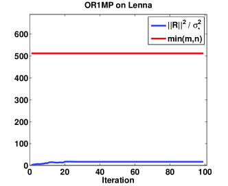
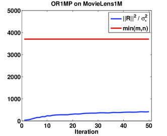
𝐑k(11min(m,n))k1YΩ,k1.formulae-sequencenormsubscript𝐑𝑘superscript11𝑚𝑛𝑘1subscriptnorm𝑌Ωfor-all𝑘1||{\bf R}_{k}||\ \leq\ \left(\sqrt{1-\frac{1}{\min(m,n)}}\right)^{k-1}\|Y\|_{\Omega},\ \ \ \forall k\geq 1.

Before proving Theorem 2, we need to establish some useful and preparatory properties of Algorithm 1. The first property says that 𝐑k+1subscript𝐑𝑘1{\bf R}_{k+1} is perpendicular to all previously generated 𝐌isubscript𝐌𝑖{\bf M}_{i} for i=1,,k𝑖1𝑘i=1,\cdots,k.

Property 3.

𝐑k+1,𝐌i=0subscript𝐑𝑘1subscript𝐌𝑖0\langle{\bf R}_{k+1},{\bf M}_{i}\rangle=0 for i=1,,k𝑖1𝑘i=1,\cdots,k.

Proof.

Recall that 𝜽ksuperscript𝜽𝑘{\bm{\theta}}^{k} is the optimal solution of problem (9). By the first-order optimality condition, one has

𝐘i=1tθik𝐌i,𝐌iΩ=0fori=1,,k,formulae-sequencesubscript𝐘subscriptsuperscript𝑡𝑖1subscriptsuperscript𝜃𝑘𝑖subscript𝐌𝑖subscript𝐌𝑖Ω0for𝑖1𝑘\langle{\bf Y}-\sum^{t}_{i=1}{\theta}^{k}_{i}{\bf M}_{i},{\bf M}_{i}\rangle_{\Omega}=0\ \mbox{for}\ i=1,\cdots,k,

which together with 𝐑k=𝐘Ω𝐗k1subscript𝐑𝑘subscript𝐘Ωsubscript𝐗𝑘1{\bf R}_{k}={\bf Y}_{\Omega}-{\bf X}_{k-1} and 𝐗k=i=1kθik(𝐌i)Ωsubscript𝐗𝑘subscriptsuperscript𝑘𝑖1subscriptsuperscript𝜃𝑘𝑖subscriptsubscript𝐌𝑖Ω{\bf X}_{k}=\sum^{k}_{i=1}{\theta}^{k}_{i}({\bf M}_{i})_{\Omega} implies that 𝐑k+1,𝐌i=0subscript𝐑𝑘1subscript𝐌𝑖0\langle{\bf R}_{k+1},{\bf M}_{i}\rangle=0 for i=1,,k𝑖1𝑘i=1,\cdots,k. ∎

The following property shows that as the number of rank-one basis matrices 𝐌isubscript𝐌𝑖{\bf M}_{i} increases during our learning process, the residual 𝐑knormsubscript𝐑𝑘\|{\bf R}_{k}\| does not increase.

Property 4.

𝐑k+1𝐑knormsubscript𝐑𝑘1normsubscript𝐑𝑘\|{\bf R}_{k+1}\|\leq\|{\bf R}_{k}\| for all k1𝑘1k\geq 1.

Proof.

We observe that for all k1𝑘1k\geq 1,

𝐑k+12=min𝜽k{𝐘i=1kθi𝐌iΩ2}min𝜽k1{𝐘i=1k1θi𝐌iΩ2}=𝐑k2,superscriptnormsubscript𝐑𝑘12subscript𝜽superscript𝑘subscriptsuperscriptnorm𝐘subscriptsuperscript𝑘𝑖1subscript𝜃𝑖subscript𝐌𝑖2Ωmissing-subexpressionsubscript𝜽superscript𝑘1subscriptsuperscriptnorm𝐘subscriptsuperscript𝑘1𝑖1subscript𝜃𝑖subscript𝐌𝑖2Ωmissing-subexpressionsuperscriptnormsubscript𝐑𝑘2\begin{array}[]{lcl}\|{\bf R}_{k+1}\|^{2}&=&\min\limits_{{\bm{\theta}}\in\Re^{k}}\{\|{\bf Y}-\sum^{k}_{i=1}{\theta}_{i}{\bf M}_{i}\|^{2}_{\Omega}\}\\[8.0pt] &\leq&\min\limits_{{\bm{\theta}}\in\Re^{k-1}}\{\|{\bf Y}-\sum^{k-1}_{i=1}{\theta}_{i}{\bf M}_{i}\|^{2}_{\Omega}\}\\[8.0pt] &=&\ \|{\bf R}_{k}\|^{2},\end{array}

and hence the conclusion holds. ∎

We next establish that {(𝐌i)Ω}i=1ksubscriptsuperscriptsubscriptsubscript𝐌𝑖Ω𝑘𝑖1\{({\bf M}_{i})_{\Omega}\}^{k}_{i=1} is linearly independent unless 𝐑k=0normsubscript𝐑𝑘0\|{\bf R}_{k}\|=0. It follows that formula (10) is well-defined and hence 𝜽ksuperscript𝜽𝑘{\bm{\theta}}^{k} is uniquely defined before the algorithm stops.

Property 5.

Suppose that 𝐑k0subscript𝐑𝑘0{\bf R}_{k}\neq 0 for some k1𝑘1k\geq 1. Then, 𝐌¯isubscript¯𝐌𝑖{\bf{\bar{M}}}_{i} has a full column rank for all ik𝑖𝑘i\leq k.

Proof.

Using Property 4 and the assumption 𝐑k0subscript𝐑𝑘0{\bf R}_{k}\neq 0 for some k1𝑘1k\geq 1, we see that 𝐑i0subscript𝐑𝑖0{\bf R}_{i}\neq 0 for all ik𝑖𝑘i\leq k. We now prove the statement of this lemma by induction on i𝑖i. Indeed, since 𝐑10subscript𝐑10{\bf R}_{1}\neq 0, we clearly have 𝐌¯10subscript¯𝐌10{\bf{\bar{M}}}_{1}\neq 0. Hence the conclusion holds for i=1𝑖1i=1. We now assume that it holds for i1<k𝑖1𝑘i-1<k and need to show that it also holds for ik𝑖𝑘i\leq k. By the induction hypothesis, 𝐌¯i1subscript¯𝐌𝑖1{\bf{\bar{M}}}_{i-1} has a full column rank. Suppose for contradiction that 𝐌¯isubscript¯𝐌𝑖{\bf{\bar{M}}}_{i} does not have a full column rank. Then, there exists 𝜶i1𝜶superscript𝑖1{\bm{\alpha}}\in\Re^{i-1} such that

(𝐌i)Ω=j=1i1αj(𝐌j)Ω,subscriptsubscript𝐌𝑖Ωsubscriptsuperscript𝑖1𝑗1subscript𝛼𝑗subscriptsubscript𝐌𝑗Ω({\bf M}_{i})_{\Omega}=\sum^{i-1}\limits_{j=1}{\alpha}_{j}({\bf M}_{j})_{\Omega},

which together with Property 3 implies that 𝐑i,𝐌i=0subscript𝐑𝑖subscript𝐌𝑖0\langle{\bf R}_{i},{\bf M}_{i}\rangle=0. It follows that

σ1(𝐑i)=uiT𝐑ivi=𝐑i,𝐌i=0,subscript𝜎1subscript𝐑𝑖subscriptsuperscript𝑢𝑇𝑖subscript𝐑𝑖subscript𝑣𝑖subscript𝐑𝑖subscript𝐌𝑖0\sigma_{1}({\bf R}_{i})=u^{T}_{i}{\bf R}_{i}v_{i}=\langle{\bf R}_{i},{\bf M}_{i}\rangle=0,

and hence 𝐑i=0subscript𝐑𝑖0{\bf R}_{i}=0, which contradicts the fact that 𝐑j0subscript𝐑𝑗0{\bf R}_{j}\neq 0 for all ji𝑗𝑖j\leq i. Therefore, 𝐌¯isubscript¯𝐌𝑖{\bf{\bar{M}}}_{i} has a full column rank and the conclusion holds for general i𝑖i. ∎

We next build a relationship between two consecutive residuals 𝐑k+1normsubscript𝐑𝑘1\|{\bf R}_{k+1}\| and 𝐑knormsubscript𝐑𝑘\|{\bf R}_{k}\|. For convenience, define θkk1=0subscriptsuperscript𝜃𝑘1𝑘0{\theta}^{k-1}_{k}=0 and let

𝜽k=𝜽k1+𝜼ksuperscript𝜽𝑘superscript𝜽𝑘1superscript𝜼𝑘{\bm{\theta}}^{k}={\bm{\theta}}^{k-1}+{\bm{\eta}}^{k}.

In view of (9), one can observe that

𝜼k=argmin𝜼i=1kηi𝐌i𝐑kΩ2.superscript𝜼𝑘subscript𝜼subscriptsuperscriptnormsuperscriptsubscript𝑖1𝑘subscript𝜂𝑖subscript𝐌𝑖subscript𝐑𝑘2Ω{\bm{\eta}}^{k}=\arg\min\limits_{{\bm{\eta}}}||\sum\limits_{i=1}^{k}{\eta}_{i}{\bf M}_{i}-{\bf R}_{k}||^{2}_{\Omega}. (11)

Let

𝐋k=i=1kηik(𝐌i)Ω.subscript𝐋𝑘subscriptsuperscript𝑘𝑖1subscriptsuperscript𝜂𝑘𝑖subscriptsubscript𝐌𝑖Ω{\bf L}_{k}=\sum^{k}_{i=1}{\eta}^{k}_{i}({\bf M}_{i})_{\Omega}. (12)

By the definition of 𝐗ksubscript𝐗𝑘{\bf X}_{k}, one can also observe that

𝐗k=𝐗k1+𝐋k,𝐑k+1=𝐑k𝐋k.subscript𝐗𝑘subscript𝐗𝑘1subscript𝐋𝑘subscript𝐑𝑘1subscript𝐑𝑘subscript𝐋𝑘\begin{array}[]{l}{\bf X}_{k}={\bf X}_{k-1}+{\bf L}_{k},\\[6.0pt] {\bf R}_{k+1}={\bf R}_{k}-{\bf L}_{k}.\end{array}
Property 6.

𝐑k+12=𝐑k2𝐋k2superscriptnormsubscript𝐑𝑘12superscriptnormsubscript𝐑𝑘2superscriptnormsubscript𝐋𝑘2||{\bf R}_{k+1}||^{2}=||{\bf R}_{k}||^{2}-||{\bf L}_{k}||^{2} and 𝐋k2𝐌k,𝐑k2superscriptnormsubscript𝐋𝑘2superscriptsubscript𝐌𝑘subscript𝐑𝑘2||{\bf L}_{k}||^{2}\geq\langle{\bf M}_{k},{\bf R}_{k}\rangle^{2}, where 𝐋ksubscript𝐋𝑘{\bf L}_{k} is defined in (12).

Proof.

Since 𝐋k=ik𝜼ik(𝐌i)Ωsubscript𝐋𝑘subscript𝑖𝑘subscriptsuperscript𝜼𝑘𝑖subscriptsubscript𝐌𝑖Ω{\bf L}_{k}=\sum_{i\leq k}{\bm{\eta}}^{k}_{i}({\bf M}_{i})_{\Omega}, it follows from Property 3 that 𝐑k+1,𝐋k=0subscript𝐑𝑘1subscript𝐋𝑘0\langle{\bf R}_{k+1},{\bf L}_{k}\rangle=0. We then have

𝐑k+12=𝐑k𝐋k2=𝐑k22𝐑k,𝐋k+𝐋k2=𝐑k22𝐑k+1+𝐋k,𝐋k+𝐋k2=𝐑k22𝐋k,𝐋k+𝐋k2=𝐑k2𝐋k2.superscriptnormsubscript𝐑𝑘12absentsuperscriptnormsubscript𝐑𝑘subscript𝐋𝑘2missing-subexpressionabsentsuperscriptnormsubscript𝐑𝑘22subscript𝐑𝑘subscript𝐋𝑘superscriptnormsubscript𝐋𝑘2missing-subexpressionabsentsuperscriptnormsubscript𝐑𝑘22subscript𝐑𝑘1subscript𝐋𝑘subscript𝐋𝑘superscriptnormsubscript𝐋𝑘2missing-subexpressionabsentsuperscriptnormsubscript𝐑𝑘22subscript𝐋𝑘subscript𝐋𝑘superscriptnormsubscript𝐋𝑘2missing-subexpressionabsentsuperscriptnormsubscript𝐑𝑘2superscriptnormsubscript𝐋𝑘2\begin{array}[]{ll}||{\bf R}_{k+1}||^{2}&=||{\bf R}_{k}-{\bf L}_{k}||^{2}\\[6.0pt] &=||{\bf R}_{k}||^{2}-2\langle{\bf R}_{k},{\bf L}_{k}\rangle+||{\bf L}_{k}||^{2}\\[6.0pt] &=||{\bf R}_{k}||^{2}-2\langle{\bf R}_{k+1}+{\bf L}_{k},{\bf L}_{k}\rangle+||{\bf L}_{k}||^{2}\\[6.0pt] &=||{\bf R}_{k}||^{2}-2\langle{\bf L}_{k},{\bf L}_{k}\rangle+||{\bf L}_{k}||^{2}\\[6.0pt] &=||{\bf R}_{k}||^{2}-||{\bf L}_{k}||^{2}.\end{array}

We next bound 𝐋k2superscriptnormsubscript𝐋𝑘2\|{\bf L}_{k}\|^{2} from below. If 𝐑k=0subscript𝐑𝑘0{\bf R}_{k}=0, 𝐋k2𝐌k,𝐑k2superscriptnormsubscript𝐋𝑘2superscriptsubscript𝐌𝑘subscript𝐑𝑘2||{\bf L}_{k}||^{2}\geq\langle{\bf M}_{k},{\bf R}_{k}\rangle^{2} clearly holds. We now suppose throughout the remaining proof that 𝐑k0subscript𝐑𝑘0{\bf R}_{k}\neq 0. It then follows from Property 5 that 𝐌¯ksubscript¯𝐌𝑘{\bf{\bar{M}}}_{k} has a full column rank. Using this fact and (11), we have

𝜼k=(𝐌¯kT𝐌¯k)1𝐌¯kT𝐫˙k,superscript𝜼𝑘superscriptsubscriptsuperscript¯𝐌𝑇𝑘subscript¯𝐌𝑘1subscriptsuperscript¯𝐌𝑇𝑘subscript˙𝐫𝑘{\bm{\eta}}^{k}=\left({\bf{\bar{M}}}^{T}_{k}{\bf{\bar{M}}}_{k}\right)^{-1}{\bf{\bar{M}}}^{T}_{k}\dot{\bf r}_{k},

where 𝐫˙ksubscript˙𝐫𝑘\dot{\bf r}_{k} is the reshaped residual vector of 𝐑ksubscript𝐑𝑘{\bf R}_{k}. Invoking that 𝐋k=ikηik(𝐌i)Ωsubscript𝐋𝑘subscript𝑖𝑘subscriptsuperscript𝜂𝑘𝑖subscriptsubscript𝐌𝑖Ω{\bf L}_{k}=\sum\limits_{i\leq k}{\eta}^{k}_{i}({\bf M}_{i})_{\Omega}, we then obtain

𝐋k2=𝐫˙kT𝐌¯k(𝐌¯kT𝐌¯k)1𝐌¯kT𝐫˙k.superscriptnormsubscript𝐋𝑘2subscriptsuperscript˙𝐫𝑇𝑘subscript¯𝐌𝑘superscriptsubscriptsuperscript¯𝐌𝑇𝑘subscript¯𝐌𝑘1subscriptsuperscript¯𝐌𝑇𝑘subscript˙𝐫𝑘||{\bf L}_{k}||^{2}=\dot{\bf r}^{T}_{k}{\bf{\bar{M}}}_{k}({\bf{\bar{M}}}^{T}_{k}{\bf{\bar{M}}}_{k})^{-1}{\bf{\bar{M}}}^{T}_{k}\dot{\bf r}_{k}. (13)

Let 𝐌¯k=𝐐𝐔subscript¯𝐌𝑘𝐐𝐔{\bf{\bar{M}}}_{k}={\bf Q}{\bf U} be the QR factorization of 𝐌¯ksubscript¯𝐌𝑘{\bf{\bar{M}}}_{k}, where 𝐐T𝐐=𝐈superscript𝐐𝑇𝐐𝐈{\bf Q}^{T}{\bf Q}={\bf I} and 𝐔𝐔{\bf U} is a k×k𝑘𝑘k\times k nonsingular upper triangular matrix. One can observe that (𝐌¯k)k=𝐦˙ksubscriptsubscript¯𝐌𝑘𝑘subscript˙𝐦𝑘({\bf{\bar{M}}}_{k})_{k}=\dot{\bf m}_{k}, where (𝐌¯k)ksubscriptsubscript¯𝐌𝑘𝑘({\bf{\bar{M}}}_{k})_{k} denotes the k𝑘k-th column of the matrix 𝐌¯ksubscript¯𝐌𝑘{\bf{\bar{M}}}_{k} and 𝐦˙ksubscript˙𝐦𝑘\dot{\bf m}_{k} is the reshaped vector of (𝐌k)Ωsubscriptsubscript𝐌𝑘Ω({\bf M}_{k})_{\Omega}. Recall that 𝐌k=𝐮k𝐯kT=1normsubscript𝐌𝑘normsubscript𝐮𝑘subscriptsuperscript𝐯𝑇𝑘1\|{\bf M}_{k}\|=\|{\bf u}_{k}{\bf v}^{T}_{k}\|=1. Hence, (𝐌¯k)k1normsubscriptsubscript¯𝐌𝑘𝑘1\|({\bf{\bar{M}}}_{k})_{k}\|\leq 1. Due to 𝐐T𝐐=𝐈superscript𝐐𝑇𝐐𝐈{\bf Q}^{T}{\bf Q}={\bf I}, 𝐌¯k=𝐐𝐔subscript¯𝐌𝑘𝐐𝐔{\bf{\bar{M}}}_{k}={\bf QU} and the definition of 𝐔𝐔\bf U, we have

0<|𝐔kk|𝐔k=(𝐌¯k)k 1.0subscript𝐔𝑘𝑘normsubscript𝐔𝑘normsubscriptsubscript¯𝐌𝑘𝑘10\ <\ |{\bf U}_{kk}|\ \leq\ \|{\bf U}_{k}\|\ =\ \|({\bf{\bar{M}}}_{k})_{k}\|\ \leq\ 1.

In addition, by Property 3, we have

𝐌¯kT𝐫˙k=[0,,0,𝐌k,𝐑k]T.subscriptsuperscript¯𝐌𝑇𝑘subscript˙𝐫𝑘superscript00subscript𝐌𝑘subscript𝐑𝑘𝑇{\bf{\bar{M}}}^{T}_{k}\dot{\bf r}_{k}=\left[0,\cdots,0,\langle{\bf M}_{k},{\bf R}_{k}\rangle\right]^{T}. (14)

Substituting 𝐌¯k=𝐐𝐔subscript¯𝐌𝑘𝐐𝐔{\bf{\bar{M}}}_{k}=\bf QU into (13), and using 𝐐𝐓𝐐=𝐈superscript𝐐𝐓𝐐𝐈\bf Q^{T}Q=I and (14), we obtain that

𝐋k2=𝐫˙kT𝐌¯k(𝐔T𝐔)1𝐌¯kT𝐫˙k=[0,,0,𝐌k,𝐑k]𝐔1𝐔T[0,,0,𝐌k,𝐑k]T=𝐌k,𝐑k2/(𝐔kk)2𝐌k,𝐑k2,superscriptnormsubscript𝐋𝑘2subscriptsuperscript˙𝐫𝑇𝑘subscript¯𝐌𝑘superscriptsuperscript𝐔𝑇𝐔1subscriptsuperscript¯𝐌𝑇𝑘subscript˙𝐫𝑘absent00subscript𝐌𝑘subscript𝐑𝑘superscript𝐔1superscript𝐔𝑇superscript00subscript𝐌𝑘subscript𝐑𝑘𝑇absentsuperscriptsubscript𝐌𝑘subscript𝐑𝑘2superscriptsubscript𝐔𝑘𝑘2superscriptsubscript𝐌𝑘subscript𝐑𝑘2\begin{array}[]{l}\|{\bf L}_{k}\|^{2}\ =\ \dot{\bf r}^{T}_{k}{\bf{\bar{M}}}_{k}({\bf U}^{T}{\bf U})^{-1}{\bf{\bar{M}}}^{T}_{k}\dot{\bf r}_{k}\\[5.0pt] =\ \left[0,\cdots,0,\langle{\bf M}_{k},{\bf R}_{k}\rangle\right]{\bf U}^{-1}{\bf U}^{-T}\left[0,\cdots,0,\langle{\bf M}_{k},{\bf R}_{k}\rangle\right]^{T}\\[5.0pt] =\ \langle{\bf M}_{k},{\bf R}_{k}\rangle^{2}/({\bf U}_{kk})^{2}\ \geq\ \langle{\bf M}_{k},{\bf R}_{k}\rangle^{2},\end{array}

where the last equality follows since 𝐔𝐔\bf U is upper triangular and the last inequality is due to |𝐔kk|1subscript𝐔𝑘𝑘1|{\bf U}_{kk}|\leq 1. ∎

We are now ready to prove Theorem 2.

of Theorem 2.

Using the definition of 𝐌ksubscript𝐌𝑘{\bf M}_{k}, we have

𝐌k,𝐑k=𝐮k(𝐯k)T,𝐑k=σ1(𝐑k)iσi2(𝐑k)rank(𝐑k)=𝐑k2rank(𝐑k)𝐑k2min(m,n).subscript𝐌𝑘subscript𝐑𝑘superscript𝐮𝑘superscriptsuperscript𝐯𝑘𝑇subscript𝐑𝑘subscript𝜎1subscript𝐑𝑘absentsubscript𝑖subscriptsuperscript𝜎2𝑖subscript𝐑𝑘ranksubscript𝐑𝑘superscriptnormsubscript𝐑𝑘2ranksubscript𝐑𝑘superscriptnormsubscript𝐑𝑘2𝑚𝑛\begin{array}[]{l}\langle{\bf M}_{k},{\bf R}_{k}\rangle\ =\ \langle{\bf u}^{k}({\bf v}^{k})^{T},{\bf R}_{k}\rangle\ =\ \sigma_{1}({\bf R}_{k})\\[8.0pt] \geq\ \sqrt{\frac{\sum_{i}\sigma^{2}_{i}({\bf R}_{k})}{\mathop{\operator@font rank}\nolimits({\bf R}_{k})}}\ =\ \sqrt{\frac{\|{\bf R}_{k}\|^{2}}{\mathop{\operator@font rank}\nolimits({\bf R}_{k})}}\ \geq\ \sqrt{\frac{\|{\bf R}_{k}\|^{2}}{\min(m,n)}}.\end{array}

Using this inequality and Property 6, we obtain that

𝐑k+12=𝐑k2𝐋k2𝐑k2𝐌k,𝐑k2(11min(m,n))𝐑k2.superscriptnormsubscript𝐑𝑘12superscriptnormsubscript𝐑𝑘2superscriptnormsubscript𝐋𝑘2superscriptnormsubscript𝐑𝑘2superscriptsubscript𝐌𝑘subscript𝐑𝑘2missing-subexpression11𝑚𝑛superscriptnormsubscript𝐑𝑘2\begin{array}[]{lcl}||{\bf R}_{k+1}||^{2}&=&||{\bf R}_{k}||^{2}-||{\bf L}_{k}||^{2}\ \leq\ ||{\bf R}_{k}||^{2}-\langle{\bf M}_{k},{\bf R}_{k}\rangle^{2}\\[8.0pt] &\leq&(1-\frac{1}{\min(m,n)})||{\bf R}_{k}||^{2}.\end{array}

In view of this relation and the fact that 𝐑1=𝐘𝛀𝟐normsubscript𝐑1subscriptsuperscriptnorm𝐘2𝛀\|{\bf R}_{1}\|=\|\bf Y\|^{2}_{\Omega}, we easily conclude that

𝐑k(11min(m,n))k1𝐘𝛀.normsubscript𝐑𝑘superscript11𝑚𝑛𝑘1subscriptnorm𝐘𝛀||{\bf R}_{k}||\ \leq\ \left(\sqrt{1-\frac{1}{\min(m,n)}}\right)^{k-1}\|\bf Y\|_{\Omega}.

This completes the proof. ∎

Remark 7.

If ΩΩ\Omega is the entire set of all indices of {(i,j),i=1,,m,j=1,,n}formulae-sequence𝑖𝑗𝑖1𝑚𝑗1𝑛\{(i,j),i=1,\cdots,m,j=1,\cdots,n\}, our orthogonal rank-one matrix pursuit algorithm equals to standard singular value decomposition using the power method. In particular, when ΩΩ\Omega is the set of all indices while the given entries are noisy values of an exact matrix, our OR1MP algorithm can help remove the noises.

Remark 8.

In a standard study of the convergence rate of the Orthogonal Matching Pursuit (OMP) or Orthogonal Greedy Algorithm (OGA), one can only get |𝐌k,𝐑k|𝐑k2subscript𝐌𝑘subscript𝐑𝑘superscriptnormsubscript𝐑𝑘2|\langle{\bf M}_{k},{\bf R}_{k}\rangle|\geq\|{\bf R}_{k}\|^{2}, which leads a sub-linear convergence. Our 𝐌ksubscript𝐌𝑘{\bf M}_{k} is a data dependent construction which is based on the top left and right singular vectors of the residual matrix 𝐑ksubscript𝐑𝑘{\bf R}_{k}. It thus has a better estimate which gives us the linear convergence.

4 An Economic Orthogonal Rank-One Matrix Pursuit Algorithm

The proposed OR1MP algorithm has to track all pursued bases and save them in the memory. It demands O(r|Ω|)𝑂𝑟ΩO(r|\Omega|) storage complexity to obtain a rank-r𝑟r estimated matrix. For large scale problems, such storage requirement is not negligible and restricts the rank of the matrix to be estimated. To adapt our algorithm to large scale problems with a large approximation rank, we simplify the orthogonal projection step by only tracking the estimated matrix 𝐗k1subscript𝐗𝑘1{\bf X}_{k-1} and the rank-one update matrix 𝐌ksubscript𝐌𝑘{\bf M}_{k}. In this case, we only need to estimate the weights for these two matrices by solving the following least squares problem:

𝜶k=argmin𝜶={α1,α2}α1𝐗k1+α2𝐌k𝐘Ω2.superscript𝜶𝑘subscript𝜶subscript𝛼1subscript𝛼2subscriptsuperscriptnormsubscript𝛼1subscript𝐗𝑘1subscript𝛼2subscript𝐌𝑘𝐘2Ω{\bm{\alpha}}^{k}=\arg\min\limits_{{\bm{\alpha}}=\{\alpha_{1},\alpha_{2}\}}||{\alpha}_{1}{\bf X}_{k-1}+{\alpha}_{2}{\bf M}_{k}-{\bf Y}||^{2}_{\Omega}. (15)

This still fully corrects all weights of the existed bases, though the correction is sub-optimal. If we write the estimated matrix as a linear combination of the bases, we have 𝐗k=i=1kθik(𝐌i)Ωsubscript𝐗𝑘subscriptsuperscript𝑘𝑖1subscriptsuperscript𝜃𝑘𝑖subscriptsubscript𝐌𝑖Ω{\bf X}_{k}=\sum^{k}_{i=1}{\theta}^{k}_{i}({\bf M}_{i})_{\Omega} with θkk=α2ksubscriptsuperscript𝜃𝑘𝑘superscriptsubscript𝛼2𝑘{\theta}^{k}_{k}={\alpha}_{2}^{k} and θik=θik1α1ksubscriptsuperscript𝜃𝑘𝑖subscriptsuperscript𝜃𝑘1𝑖superscriptsubscript𝛼1𝑘{\theta}^{k}_{i}={\theta}^{k-1}_{i}{\alpha}_{1}^{k}, for i<k𝑖𝑘i<k. The detailed procedure of this simplified method is given in Algorithm 2.

Algorithm 2 Economic Orthogonal Rank-One Matrix Pursuit (EOR1MP)
  Input: 𝐘Ωsubscript𝐘Ω{\bf Y}_{\Omega} and stopping criterion.
  Initialize: Set 𝐗0=0subscript𝐗00{\bf X}_{0}=0, 𝜽0=0superscript𝜽00{\bm{\theta}}^{0}=0 and k=1𝑘1k=1.
  repeat
     Step 1: Find a pair of top left and right singular vectors (𝐮k,𝐯k)subscript𝐮𝑘subscript𝐯𝑘({\bf u}_{k},{\bf v}_{k}) of the observed residual matrix 𝐑k=𝐘Ω𝐗k1subscript𝐑𝑘subscript𝐘Ωsubscript𝐗𝑘1{\bf R}_{k}={\bf Y}_{\Omega}-{\bf X}_{k-1} and set 𝐌k=𝐮k(𝐯k)Tsubscript𝐌𝑘subscript𝐮𝑘superscriptsubscript𝐯𝑘𝑇{\bf M}_{k}={\bf u}_{k}({\bf v}_{k})^{T}.
     Step 2: Compute the optimal weights 𝜶ksuperscript𝜶𝑘{\bm{\alpha}}^{k} for 𝐗k1subscript𝐗𝑘1{\bf X}_{k-1} and 𝐌ksubscript𝐌𝑘{\bf M}_{k} by solving: argmin𝜶α1𝐗k1+α2(𝐌k)Ω𝐘Ω2subscript𝜶superscriptnormsubscript𝛼1subscript𝐗𝑘1subscript𝛼2subscriptsubscript𝐌𝑘Ωsubscript𝐘Ω2\arg\min\limits_{\bm{\alpha}}||{\alpha}_{1}{\bf X}_{k-1}+{\alpha}_{2}({\bf M}_{k})_{\Omega}-{\bf Y}_{\Omega}||^{2}.
     Step 3: Set 𝐗k=α1k𝐗k1+α2k(𝐌k)Ωsubscript𝐗𝑘superscriptsubscript𝛼1𝑘subscript𝐗𝑘1superscriptsubscript𝛼2𝑘subscriptsubscript𝐌𝑘Ω{\bf X}_{k}={\alpha}_{1}^{k}{\bf X}_{k-1}+{\alpha}_{2}^{k}({\bf M}_{k})_{\Omega}; θkk=α2ksubscriptsuperscript𝜃𝑘𝑘superscriptsubscript𝛼2𝑘{\theta}^{k}_{k}={\alpha}_{2}^{k} and θik=θik1α1ksubscriptsuperscript𝜃𝑘𝑖subscriptsuperscript𝜃𝑘1𝑖superscriptsubscript𝛼1𝑘{\theta}^{k}_{i}={\theta}^{k-1}_{i}{\alpha}_{1}^{k} for i<k𝑖𝑘i<k; kk+1𝑘𝑘1k\leftarrow k+1.
  until  stopping criterion is satisfied
  Output: Constructed matrix 𝐘^=i=1kθik𝐌i^𝐘subscriptsuperscript𝑘𝑖1subscriptsuperscript𝜃𝑘𝑖subscript𝐌𝑖\hat{\bf Y}=\sum^{k}_{i=1}{\theta}^{k}_{i}{\bf M}_{i}.

The proposed economic orthogonal rank-one matrix pursuit algorithm (EOR1MP) uses the same amount of storage as the greedy algorithms [17, 42], which is significantly smaller than that required by our OR1MP algorithm, Algorithm 1. Interestingly, we can show that the EOR1MP algorithm is still convergent and retains the linear convergence rate. The main result is given in the following theorem.

Theorem 9.

Algorithm 2, the economic orthogonal rank-one matrix pursuit algorithm satisfies

𝐑k(11min(m,n))k1YΩ,k1.formulae-sequencenormsubscript𝐑𝑘superscript11𝑚𝑛𝑘1subscriptnorm𝑌Ωfor-all𝑘1||{\bf R}_{k}||\ \leq\ \left(\sqrt{1-\frac{1}{\min(m,n)}}\right)^{k-1}\|Y\|_{\Omega},\ \ \ \forall k\geq 1.

Before proving Theorem 9, we present several useful properties of our Algorithm 2. The first property says that 𝐑k+1subscript𝐑𝑘1{\bf R}_{k+1} is perpendicular to matrix 𝐗k1subscript𝐗𝑘1{\bf X}_{k-1} and matrix 𝐌ksubscript𝐌𝑘{\bf M}_{k}.

Property 10.

𝐑k+1,𝐗k1=0subscript𝐑𝑘1subscript𝐗𝑘10\langle{\bf R}_{k+1},{\bf X}_{k-1}\rangle=0 and 𝐑k+1,𝐌k=0subscript𝐑𝑘1subscript𝐌𝑘0\langle{\bf R}_{k+1},{\bf M}_{k}\rangle=0.

Proof.

Recall that 𝜶ksuperscript𝜶𝑘{\bm{\alpha}}^{k} is the optimal solution of problem (15). By the first-order optimality condition according to 𝐗k1subscript𝐗𝑘1{\bf X}_{k-1} and 𝐌ksubscript𝐌𝑘{\bf M}_{k}, one has

𝐘α1k𝐗k1α2k𝐌k,𝐗k1Ω=0,subscript𝐘superscriptsubscript𝛼1𝑘subscript𝐗𝑘1superscriptsubscript𝛼2𝑘subscript𝐌𝑘subscript𝐗𝑘1Ω0\langle{\bf Y}-{\alpha}_{1}^{k}{\bf X}_{k-1}-{\alpha}_{2}^{k}{\bf M}_{k},{\bf X}_{k-1}\rangle_{\Omega}=0,

and

𝐘α1k𝐗k1α2k𝐌k,𝐌kΩ=0,subscript𝐘superscriptsubscript𝛼1𝑘subscript𝐗𝑘1superscriptsubscript𝛼2𝑘subscript𝐌𝑘subscript𝐌𝑘Ω0\langle{\bf Y}-{\alpha}_{1}^{k}{\bf X}_{k-1}-{\alpha}_{2}^{k}{\bf M}_{k},{\bf M}_{k}\rangle_{\Omega}=0,

which together with 𝐑k=𝐘Ω𝐗k1subscript𝐑𝑘subscript𝐘Ωsubscript𝐗𝑘1{\bf R}_{k}={\bf Y}_{\Omega}-{\bf X}_{k-1} implies that 𝐑k+1,𝐗k1=0subscript𝐑𝑘1subscript𝐗𝑘10\langle{\bf R}_{k+1},{\bf X}_{k-1}\rangle=0 and 𝐑k+1,𝐌k=0subscript𝐑𝑘1subscript𝐌𝑘0\langle{\bf R}_{k+1},{\bf M}_{k}\rangle=0. ∎

Property 11.

𝐑k+12=𝐘Ω2𝐗k2superscriptnormsubscript𝐑𝑘12superscriptnormsubscript𝐘Ω2superscriptnormsubscript𝐗𝑘2\|{\bf R}_{k+1}\|^{2}=\|{\bf Y}_{\Omega}\|^{2}-\|{\bf X}_{k}\|^{2} for all k1𝑘1k\geq 1.

Proof.

We observe that for all k1𝑘1k\geq 1,

𝐘Ω2=𝐑k+1+𝐗k2=𝐑k+12+𝐗k2+2𝐑k+1,𝐗k=𝐑k+12+𝐗k2superscriptnormsubscript𝐘Ω2superscriptnormsubscript𝐑𝑘1subscript𝐗𝑘2missing-subexpressionsuperscriptnormsubscript𝐑𝑘12superscriptnormsubscript𝐗𝑘22subscript𝐑𝑘1subscript𝐗𝑘missing-subexpressionsuperscriptnormsubscript𝐑𝑘12superscriptnormsubscript𝐗𝑘2\begin{array}[]{lcl}\|{\bf Y}_{\Omega}\|^{2}&=&\|{\bf R}_{k+1}+{\bf X}_{k}\|^{2}\\[8.0pt] &=&\|{\bf R}_{k+1}\|^{2}+\|{\bf X}_{k}\|^{2}+2\langle{\bf R}_{k+1},{\bf X}_{k}\rangle\\[8.0pt] &=&\|{\bf R}_{k+1}\|^{2}+\|{\bf X}_{k}\|^{2}\end{array}

as 𝐑k+1,𝐗k=α1k𝐑k+1,𝐗k1+α2k𝐑k+1,𝐌k=0subscript𝐑𝑘1subscript𝐗𝑘superscriptsubscript𝛼1𝑘subscript𝐑𝑘1subscript𝐗𝑘1superscriptsubscript𝛼2𝑘subscript𝐑𝑘1subscript𝐌𝑘0\langle{\bf R}_{k+1},{\bf X}_{k}\rangle={\alpha}_{1}^{k}\langle{\bf R}_{k+1},{\bf X}_{k-1}\rangle+{\alpha}_{2}^{k}\langle{\bf R}_{k+1},{\bf M}_{k}\rangle=0, and hence the conclusion holds. ∎

The following property shows that as the number of rank-one basis matrices 𝐌isubscript𝐌𝑖{\bf M}_{i} increases during our iterative process, the residual 𝐑knormsubscript𝐑𝑘\|{\bf R}_{k}\| decreases.

Property 12.

𝐑k+1𝐑knormsubscript𝐑𝑘1normsubscript𝐑𝑘\|{\bf R}_{k+1}\|\leq\|{\bf R}_{k}\| for all k1𝑘1k\geq 1.

Proof.

We observe that for all k1𝑘1k\geq 1,

𝐑k2=min𝜶2𝐘α1𝐗k2α2𝐌k1Ω2=𝐘(α1k1𝐗k2+α2k1𝐌k1)Ω2min𝜶2𝐘α1(α1k1𝐗k2+α2k1𝐌k1)α2𝐌kΩ2=min𝜶2𝐘α1𝐗k1α2𝐌kΩ2=𝐑k+12,superscriptnormsubscript𝐑𝑘2subscript𝜶superscript2subscriptsuperscriptnorm𝐘subscript𝛼1subscript𝐗𝑘2subscript𝛼2subscript𝐌𝑘12Ωmissing-subexpressionsubscriptsuperscriptnorm𝐘superscriptsubscript𝛼1𝑘1subscript𝐗𝑘2superscriptsubscript𝛼2𝑘1subscript𝐌𝑘12Ωmissing-subexpressionsubscript𝜶superscript2subscriptsuperscriptnorm𝐘subscript𝛼1superscriptsubscript𝛼1𝑘1subscript𝐗𝑘2superscriptsubscript𝛼2𝑘1subscript𝐌𝑘1subscript𝛼2subscript𝐌𝑘2Ωmissing-subexpressionsubscript𝜶superscript2subscriptsuperscriptnorm𝐘subscript𝛼1subscript𝐗𝑘1subscript𝛼2subscript𝐌𝑘2Ωmissing-subexpressionsuperscriptnormsubscript𝐑𝑘12\begin{array}[]{lcl}\|{\bf R}_{k}\|^{2}&=&\min\limits_{{\bm{\alpha}}\in\Re^{2}}\|{\bf Y}-{\alpha}_{1}{\bf X}_{k-2}-{\alpha}_{2}{\bf M}_{k-1}\|^{2}_{\Omega}\\[8.0pt] &=&{\|{\bf Y}-({\alpha}_{1}^{k-1}{\bf X}_{k-2}+{\alpha}_{2}^{k-1}{\bf M}_{k-1})\|^{2}_{\Omega}}\\[8.0pt] &\geq&\min\limits_{{\bm{\alpha}}\in\Re^{2}}\|{\bf Y}-{\alpha}_{1}({\alpha}_{1}^{k-1}{\bf X}_{k-2}+{\alpha}_{2}^{k-1}{\bf M}_{k-1})-{\alpha}_{2}{\bf M}_{k}\|^{2}_{\Omega}\\[8.0pt] &=&\min\limits_{{\bm{\alpha}}\in\Re^{2}}\|{\bf Y}-{\alpha}_{1}{\bf X}_{k-1}-{\alpha}_{2}{\bf M}_{k}\|^{2}_{\Omega}\\[8.0pt] &=&\ \|{\bf R}_{k+1}\|^{2},\end{array}

and hence the conclusion holds. ∎

Let

𝐀k=𝐁kT𝐁k=[𝐗k1,𝐗k1𝐗k1,𝐌k𝐌k,𝐗k1𝐌k,𝐌kΩ]subscript𝐀𝑘subscriptsuperscript𝐁𝑇𝑘subscript𝐁𝑘matrixsubscript𝐗𝑘1subscript𝐗𝑘1subscript𝐗𝑘1subscript𝐌𝑘subscript𝐌𝑘subscript𝐗𝑘1subscriptsubscript𝐌𝑘subscript𝐌𝑘Ωmissing-subexpression{\bf A}_{k}={\bf B}^{T}_{k}{\bf B}_{k}=\begin{array}[]{lc}\begin{bmatrix}\langle{\bf X}_{k-1},{\bf X}_{k-1}\rangle&\langle{\bf X}_{k-1},{\bf M}_{k}\rangle\\[6.0pt] \langle{\bf M}_{k},{\bf X}_{k-1}\rangle&\langle{\bf M}_{k},{\bf M}_{k}\rangle_{\Omega}\end{bmatrix}\end{array}

and 𝐁k=[vec(𝐗k1),vec((𝐌k)Ω)]subscript𝐁𝑘𝑣𝑒𝑐subscript𝐗𝑘1𝑣𝑒𝑐subscriptsubscript𝐌𝑘Ω{\bf B}_{k}=[vec({\bf X}_{k-1}),vec(({\bf M}_{k})_{\Omega})]. The solution of problem (15) is 𝜶k=𝐀k1𝐁kTvec(𝐘Ω)superscript𝜶𝑘superscriptsubscript𝐀𝑘1subscriptsuperscript𝐁𝑇𝑘𝑣𝑒𝑐subscript𝐘Ω{\bm{\alpha}}^{k}={\bf A}_{k}^{-1}{\bf B}^{T}_{k}vec({\bf Y}_{\Omega}). We next establish that vec(𝐗k1)𝑣𝑒𝑐subscript𝐗𝑘1vec({\bf X}_{k-1}) and vec((𝐌k)Ω)𝑣𝑒𝑐subscriptsubscript𝐌𝑘Ωvec(({\bf M}_{k})_{\Omega}) are linearly independent unless 𝐑k=0normsubscript𝐑𝑘0\|{\bf R}_{k}\|=0. It follows that 𝐀ksubscript𝐀𝑘{\bf A}_{k} is invertible and hence 𝜶ksuperscript𝜶𝑘{\bm{\alpha}}^{k} is uniquely defined before the algorithm stops.

Property 13.

If 𝐗k1=β(𝐌k)Ωsubscript𝐗𝑘1𝛽subscriptsubscript𝐌𝑘Ω{\bf X}_{k-1}=\beta({\bf M}_{k})_{\Omega} for some β0𝛽0\beta\not=0, then 𝐑k+1=𝐑knormsubscript𝐑𝑘1normsubscript𝐑𝑘\|{\bf R}_{k+1}\|=\|{\bf R}_{k}\|.

Proof.

If 𝐗k1=β(𝐌k)Ωsubscript𝐗𝑘1𝛽subscriptsubscript𝐌𝑘Ω{\bf X}_{k-1}=\beta({\bf M}_{k})_{\Omega} with nonzero β𝛽\beta, we get

𝐑k+12=min𝜶2𝐘α1𝐗k1α2𝐌kΩ2=min𝜶2𝐘(α1+α2/β)𝐗k1Ω2=minγ𝐘γ𝐗k1Ω2=minγ𝐘γα1k1𝐗k2γα2k1𝐌k1Ω2min𝜸2𝐘γ1𝐗k2γ2𝐌k1Ω2=𝐘𝐗k1Ω2=𝐑k2.superscriptnormsubscript𝐑𝑘12subscript𝜶superscript2subscriptsuperscriptnorm𝐘subscript𝛼1subscript𝐗𝑘1subscript𝛼2subscript𝐌𝑘2Ωmissing-subexpressionsubscript𝜶superscript2subscriptsuperscriptnorm𝐘subscript𝛼1subscript𝛼2𝛽subscript𝐗𝑘12Ωmissing-subexpressionsubscript𝛾subscriptsuperscriptnorm𝐘𝛾subscript𝐗𝑘12Ωmissing-subexpressionsubscript𝛾subscriptsuperscriptnorm𝐘𝛾subscriptsuperscript𝛼𝑘11subscript𝐗𝑘2𝛾subscriptsuperscript𝛼𝑘12subscript𝐌𝑘12Ωmissing-subexpressionsubscript𝜸superscript2subscriptsuperscriptnorm𝐘subscript𝛾1subscript𝐗𝑘2subscript𝛾2subscript𝐌𝑘12Ωmissing-subexpressionsubscriptsuperscriptnorm𝐘subscript𝐗𝑘12Ωmissing-subexpressionsuperscriptnormsubscript𝐑𝑘2\begin{array}[]{lcl}\|{\bf R}_{k+1}\|^{2}&=&\min\limits_{{\bm{\alpha}}\in\Re^{2}}\|{\bf Y}-{\alpha}_{1}{\bf X}_{k-1}-{\alpha}_{2}{\bf M}_{k}\|^{2}_{\Omega}\\[8.0pt] &=&\min\limits_{{\bm{\alpha}}\in\Re^{2}}\|{\bf Y}-({\alpha}_{1}+{\alpha}_{2}/\beta){\bf X}_{k-1}\|^{2}_{\Omega}\\[8.0pt] &=&\min\limits_{\gamma\in\Re}\|{\bf Y}-\gamma{\bf X}_{k-1}\|^{2}_{\Omega}\\[8.0pt] &=&\min\limits_{\gamma\in\Re}\|{\bf Y}-\gamma{\alpha}^{k-1}_{1}{\bf X}_{k-2}-\gamma{\alpha}^{k-1}_{2}{\bf M}_{k-1}\|^{2}_{\Omega}\\[8.0pt] &\geq&\min\limits_{{\bm{\gamma}}\in\Re^{2}}\|{\bf Y}-{\gamma}_{1}{\bf X}_{k-2}-{\gamma}_{2}{\bf M}_{k-1}\|^{2}_{\Omega}\\[8.0pt] &=&\|{\bf Y}-{\bf X}_{k-1}\|^{2}_{\Omega}\\[8.0pt] &=&\|{\bf R}_{k}\|^{2}.\end{array}

and hence the conclusion holds with 𝐑k2𝐑k+12superscriptnormsubscript𝐑𝑘2superscriptnormsubscript𝐑𝑘12\|{\bf R}_{k}\|^{2}\geq\|{\bf R}_{k+1}\|^{2} given in Property 12. ∎

Property 14.

Let σ1(𝐑k)subscript𝜎1subscript𝐑𝑘\sigma_{1}({\bf R}_{k}) be the maximum singular value of 𝐑ksubscript𝐑𝑘{\bf R}_{k}. 𝐌k,𝐑k=σ1(𝐑k)𝐑kmin(m,n)subscript𝐌𝑘subscript𝐑𝑘subscript𝜎1subscript𝐑𝑘normsubscript𝐑𝑘𝑚𝑛\langle{\bf M}_{k},{\bf R}_{k}\rangle=\sigma_{1}({\bf R}_{k})\geq\frac{\|{\bf R}_{k}\|}{\sqrt{\min(m,n)}} for all k1𝑘1k\geq 1.

Proof.

The optimum 𝐌ksubscript𝐌𝑘{\bf M}_{k} in our algorithm satisfies

𝐌k,𝐑k=maxrank(𝐌)=1𝐌,𝐑k=σ1(𝐑k).subscript𝐌𝑘subscript𝐑𝑘subscript𝑟𝑎𝑛𝑘𝐌1𝐌subscript𝐑𝑘subscript𝜎1subscript𝐑𝑘\langle{\bf M}_{k},{\bf R}_{k}\rangle=\max\limits_{rank({\bf M})=1}\langle{\bf M},{\bf R}_{k}\rangle=\sigma_{1}({\bf R}_{k}).

Using the fact that rank(𝐑k)σ1(𝐑k)𝐑k𝑟𝑎𝑛𝑘subscript𝐑𝑘subscript𝜎1subscript𝐑𝑘normsubscript𝐑𝑘\sqrt{rank({\bf R}_{k})}\sigma_{1}({\bf R}_{k})\geq\|{\bf R}_{k}\| and rank(𝐑k)min(m,n)𝑟𝑎𝑛𝑘subscript𝐑𝑘𝑚𝑛rank({\bf R}_{k})\leq\min(m,n), we get the conclusion. ∎

Property 15.

Suppose that 𝐑k0subscript𝐑𝑘0{\bf R}_{k}\neq 0 for some k1𝑘1k\geq 1. Then, 𝐗k1β(𝐌k)Ωsubscript𝐗𝑘1𝛽subscriptsubscript𝐌𝑘Ω{\bf X}_{k-1}\not=\beta({\bf M}_{k})_{\Omega} for all β0𝛽0\beta\not=0.

Proof.

If 𝐗k1=β(𝐌k)Ωsubscript𝐗𝑘1𝛽subscriptsubscript𝐌𝑘Ω{\bf X}_{k-1}=\beta({\bf M}_{k})_{\Omega} with β0𝛽0\beta\not=0, we have

𝐑k+12=𝐘𝐗kΩ2=min𝜶2𝐘α1𝐗k1α2𝐌kΩ2=min𝜶2𝐘(α1+α2/β)𝐗k1Ω2=minγ𝐘γ𝐗k1Ω2=𝐘γk𝐗k1Ω2=𝐑k2=𝐘𝐗k1Ω2.superscriptnormsubscript𝐑𝑘12subscriptsuperscriptnorm𝐘subscript𝐗𝑘2Ωmissing-subexpressionsubscript𝜶superscript2subscriptsuperscriptnorm𝐘subscript𝛼1subscript𝐗𝑘1subscript𝛼2subscript𝐌𝑘2Ωmissing-subexpressionsubscript𝜶superscript2subscriptsuperscriptnorm𝐘subscript𝛼1subscript𝛼2𝛽subscript𝐗𝑘12Ωmissing-subexpressionsubscript𝛾subscriptsuperscriptnorm𝐘𝛾subscript𝐗𝑘12Ωmissing-subexpressionsubscriptsuperscriptnorm𝐘superscript𝛾𝑘subscript𝐗𝑘12Ωmissing-subexpressionsuperscriptnormsubscript𝐑𝑘2missing-subexpressionsubscriptsuperscriptnorm𝐘subscript𝐗𝑘12Ω\begin{array}[]{lcl}\|{\bf R}_{k+1}\|^{2}&=&\|{\bf Y}-{\bf X}_{k}\|^{2}_{\Omega}\\[8.0pt] &=&\min\limits_{{\bm{\alpha}}\in\Re^{2}}\|{\bf Y}-{\alpha}_{1}{\bf X}_{k-1}-{\alpha}_{2}{\bf M}_{k}\|^{2}_{\Omega}\\[8.0pt] &=&\min\limits_{{\bm{\alpha}}\in\Re^{2}}\|{\bf Y}-({\alpha}_{1}+{\alpha}_{2}/\beta){\bf X}_{k-1}\|^{2}_{\Omega}\\[8.0pt] &=&\min\limits_{\gamma\in\Re}\|{\bf Y}-\gamma{\bf X}_{k-1}\|^{2}_{\Omega}\\[8.0pt] &=&\|{\bf Y}-\gamma^{k}{\bf X}_{k-1}\|^{2}_{\Omega}\\[8.0pt] &=&\|{\bf R}_{k}\|^{2}\\[8.0pt] &=&\|{\bf Y}-{\bf X}_{k-1}\|^{2}_{\Omega}.\end{array}

As 𝐑k0subscript𝐑𝑘0{\bf R}_{k}\neq 0, we have (𝐌k)Ω0subscriptsubscript𝐌𝑘Ω0({\bf M}_{k})_{\Omega}\neq 0 and 𝐗k10subscript𝐗𝑘10{\bf X}_{k-1}\neq 0. Then from the above equality, we conclude that γk=1superscript𝛾𝑘1\gamma^{k}=1 is the unique optimal solution of the minimization in terms of γ𝛾\gamma, thus we obtain its first-order optimality condition: 𝐗k1,𝐑k=0subscript𝐗𝑘1subscript𝐑𝑘0\langle{\bf X}_{k-1},{\bf R}_{k}\rangle=0. However, this contradicts with

𝐗k1,𝐑k=β𝐌k,𝐑k=βσ1(𝐑k)0.subscript𝐗𝑘1subscript𝐑𝑘𝛽subscript𝐌𝑘subscript𝐑𝑘𝛽subscript𝜎1subscript𝐑𝑘0\langle{\bf X}_{k-1},{\bf R}_{k}\rangle=\beta\langle{\bf M}_{k},{\bf R}_{k}\rangle=\beta\sigma_{1}({\bf R}_{k})\not=0.

The complete the proof. ∎

We next build a relationship between two consecutive residuals 𝐑k+1normsubscript𝐑𝑘1\|{\bf R}_{k+1}\| and 𝐑knormsubscript𝐑𝑘\|{\bf R}_{k}\|.

Property 16.

𝐑k+12𝐑k2σ12(𝐑k)𝐌k,𝐌kΩsuperscriptnormsubscript𝐑𝑘12superscriptnormsubscript𝐑𝑘2subscriptsuperscript𝜎21subscript𝐑𝑘subscriptsubscript𝐌𝑘subscript𝐌𝑘Ω\|{\bf R}_{k+1}\|^{2}\leq\|{\bf R}_{k}\|^{2}-\frac{\sigma^{2}_{1}({\bf R}_{k})}{\langle{\bf M}_{k},{\bf M}_{k}\rangle_{\Omega}}.

Proof.
𝐑k+12=min𝜶2𝐘α1𝐗k1α2𝐌kΩ2minα2𝐘𝐗k1α2𝐌kΩ2=minα2𝐑kα2𝐌kΩ2.superscriptnormsubscript𝐑𝑘12subscript𝜶superscript2subscriptsuperscriptnorm𝐘subscript𝛼1subscript𝐗𝑘1subscript𝛼2subscript𝐌𝑘2Ωmissing-subexpressionsubscriptsubscript𝛼2subscriptsuperscriptnorm𝐘subscript𝐗𝑘1subscript𝛼2subscript𝐌𝑘2Ωmissing-subexpressionsubscriptsubscript𝛼2subscriptsuperscriptnormsubscript𝐑𝑘subscript𝛼2subscript𝐌𝑘2Ω\begin{array}[]{lcl}\|{\bf R}_{k+1}\|^{2}&=&\min\limits_{{\bm{\alpha}}\in\Re^{2}}\|{\bf Y}-{\alpha}_{1}{\bf X}_{k-1}-{\alpha}_{2}{\bf M}_{k}\|^{2}_{\Omega}\\[8.0pt] &\leq&\min\limits_{{\alpha}_{2}\in\Re}\|{\bf Y}-{\bf X}_{k-1}-{\alpha}_{2}{\bf M}_{k}\|^{2}_{\Omega}\\[8.0pt] &=&\min\limits_{{\alpha}_{2}\in\Re}\|{\bf R}_{k}-{\alpha}_{2}{\bf M}_{k}\|^{2}_{\Omega}.\end{array}

This has a closed form solution as α2=𝐑k,𝐌k𝐌k,𝐌kΩsubscriptsuperscript𝛼2subscript𝐑𝑘subscript𝐌𝑘subscriptsubscript𝐌𝑘subscript𝐌𝑘Ω{\alpha}^{*}_{2}=\frac{\langle{\bf R}_{k},{\bf M}_{k}\rangle}{\langle{\bf M}_{k},{\bf M}_{k}\rangle_{\Omega}}. Plugging this optimum α2subscriptsuperscript𝛼2{\alpha}^{*}_{2} back into the formulation, we get

𝐑k+12𝐑k𝐑k,𝐌k𝐌k,𝐌k𝐌kΩ2=𝐑k2𝐑k,𝐌k2𝐌k,𝐌kΩ=𝐑k2σ12(𝐑k)𝐌k,𝐌kΩ.superscriptnormsubscript𝐑𝑘12subscriptsuperscriptnormsubscript𝐑𝑘subscript𝐑𝑘subscript𝐌𝑘subscript𝐌𝑘subscript𝐌𝑘subscript𝐌𝑘2Ωmissing-subexpressionsuperscriptnormsubscript𝐑𝑘2superscriptsubscript𝐑𝑘subscript𝐌𝑘2subscriptsubscript𝐌𝑘subscript𝐌𝑘Ωmissing-subexpressionsuperscriptnormsubscript𝐑𝑘2subscriptsuperscript𝜎21subscript𝐑𝑘subscriptsubscript𝐌𝑘subscript𝐌𝑘Ω\begin{array}[]{lcl}\|{\bf R}_{k+1}\|^{2}&\leq&\|{\bf R}_{k}-\frac{\langle{\bf R}_{k},{\bf M}_{k}\rangle}{\langle{\bf M}_{k},{\bf M}_{k}\rangle}{\bf M}_{k}\|^{2}_{\Omega}\\[8.0pt] &=&\|{\bf R}_{k}\|^{2}-\frac{\langle{\bf R}_{k},{\bf M}_{k}\rangle^{2}}{\langle{\bf M}_{k},{\bf M}_{k}\rangle_{\Omega}}\\[8.0pt] &=&\|{\bf R}_{k}\|^{2}-\frac{\sigma^{2}_{1}({\bf R}_{k})}{\langle{\bf M}_{k},{\bf M}_{k}\rangle_{\Omega}}.\end{array}

This completes the proof. ∎

We are now ready to prove Theorem 9.

of Theorem 9.

Using the definition of 𝐌ksubscript𝐌𝑘{\bf M}_{k} with its normalization property 𝐌k,𝐌kΩ1subscriptsubscript𝐌𝑘subscript𝐌𝑘Ω1{\langle{\bf M}_{k},{\bf M}_{k}\rangle_{\Omega}}\leq 1, Property 16 and Property 14, we obtain that

𝐑k+12𝐑k2σ12(𝐑k)𝐌k,𝐌kΩ𝐑k2σ12(𝐑k)(11min(m,n))𝐑k2.superscriptnormsubscript𝐑𝑘12superscriptnormsubscript𝐑𝑘2subscriptsuperscript𝜎21subscript𝐑𝑘subscriptsubscript𝐌𝑘subscript𝐌𝑘Ωsuperscriptnormsubscript𝐑𝑘2subscriptsuperscript𝜎21subscript𝐑𝑘missing-subexpression11𝑚𝑛superscriptnormsubscript𝐑𝑘2\begin{array}[]{lcl}||{\bf R}_{k+1}||^{2}&\leq&||{\bf R}_{k}||^{2}-\frac{\sigma^{2}_{1}({\bf R}_{k})}{\langle{\bf M}_{k},{\bf M}_{k}\rangle_{\Omega}}\ \leq\ ||{\bf R}_{k}||^{2}-{\sigma^{2}_{1}({\bf R}_{k})}\\[8.0pt] &\leq&\left(1-\frac{1}{\min(m,n)}\right)||{\bf R}_{k}||^{2}.\end{array}

In view of this relation and the fact that 𝐑1=𝐘𝛀𝟐normsubscript𝐑1subscriptsuperscriptnorm𝐘2𝛀\|{\bf R}_{1}\|=\|\bf Y\|^{2}_{\Omega}, we easily conclude that

𝐑k(11min(m,n))k1𝐘𝛀.normsubscript𝐑𝑘superscript11𝑚𝑛𝑘1subscriptnorm𝐘𝛀||{\bf R}_{k}||\ \leq\ \left(\sqrt{1-\frac{1}{\min(m,n)}}\right)^{k-1}\|\bf Y\|_{\Omega}.

This completes the proof. ∎

5 An Extension to the Matrix Sensing Problem and Its Convergence Analysis

In this section, we extend our algorithms to deal with the following matrix sensing problem (cf. [36, 25, 18, 19]):

min𝐗n×m rank (𝐗):𝒜(𝐗)=𝒜(𝐘),:subscript𝐗superscript𝑛𝑚 rank 𝐗𝒜𝐗𝒜𝐘\min_{{\bf X}\in\Re^{n\times m}}\hbox{ rank }({\bf X}):{\cal A}({\bf X})={\cal A}({\bf Y}), (16)

where 𝐘𝐘{\bf Y} is a target low rank matrix and 𝒜𝒜{\cal A} is a linear operator, e.g., 𝒜𝒜{\cal A} consists of vector pairs (𝐟i,𝐠i),i=1,,dformulae-sequencesubscript𝐟𝑖subscript𝐠𝑖𝑖1𝑑({\bf f}_{i},{\bf g}_{i}),i=1,\cdots,d such that 𝐟i𝐗𝐠i=𝐟i𝐘𝐠i,i=1,,dformulae-sequencesuperscriptsubscript𝐟𝑖topsubscript𝐗𝐠𝑖superscriptsubscript𝐟𝑖topsubscript𝐘𝐠𝑖𝑖1𝑑{\bf f}_{i}^{\top}{\bf X}{\bf g}_{i}={\bf f}_{i}^{\top}{\bf Y}{\bf g}_{i},i=1,\cdots,d are given constraints. Clearly, the matrix completion studied in the previous sections is a special case of the above problem by setting the linear operator 𝒜𝒜\mathcal{A} to be the observation operator PΩsubscript𝑃ΩP_{\Omega}.

Let us explain how to use our algorithms to solve this matrix sensing problem (16). Recall a linear operator vec which maps a matrix 𝐗𝐗{\bf X} of size n×m𝑛𝑚n\times m to a vector vec(𝐗)vec𝐗\hbox{vec}({\bf X}) of size mn×1𝑚𝑛1mn\times 1. We now define an inverse operator matmnsubscriptmat𝑚𝑛\hbox{mat}_{mn} which converts a vector 𝐯𝐯{\bf v} of size mn×1𝑚𝑛1mn\times 1 to a matrix 𝐕=matmn(𝐯)𝐕subscriptmat𝑚𝑛𝐯{\bf V}=\hbox{mat}_{mn}({\bf v}) of size n×m𝑛𝑚n\times m. Note that when 𝐗𝐗{\bf X} is vectorized into vec(𝐗)vec𝐗\hbox{vec}({\bf X}), the linear operator 𝒜𝒜{\cal A} can be expressed in terms of matrix 𝐀𝐀{\bf A}. That is, 𝒜(𝐗)=𝒜(𝐘)𝒜𝐗𝒜𝐘{\cal A}({\bf X})={\cal A}({\bf Y}) can be rewritten as 𝐀(vec(𝐗))=𝐀(vec(𝐘))𝐀vec𝐗𝐀vec𝐘{\bf A}(\hbox{vec}({\bf X}))={\bf A}(\hbox{vec}({\bf Y})). For convenience, we can write 𝒜=𝐀vec𝒜𝐀vec{\cal A}={\bf A}\hbox{vec}. It is clear that 𝐀𝐀{\bf A} is a matrix of size d×mn𝑑𝑚𝑛d\times mn. Certainly, one can find its pseudo inverse 𝒜superscript𝒜{\cal A}^{\dagger} which is 𝐀(𝐀𝐀)1superscript𝐀topsuperscriptsuperscript𝐀𝐀top1{\bf A}^{\top}({\bf A}{\bf A}^{\top})^{-1} as we have assumed that 𝐀𝐀{\bf A} is of full row rank. We note that since d<<mnmuch-less-than𝑑𝑚𝑛d<<mn, 𝐀𝐀=𝐈dsuperscript𝐀𝐀subscript𝐈𝑑{\bf A}{\bf A}^{\dagger}={\bf I}_{d} while 𝐀𝐀𝐈mnsuperscript𝐀𝐀subscript𝐈𝑚𝑛{\bf A}^{\dagger}{\bf A}\not={\bf I}_{mn}, where 𝐈dsubscript𝐈𝑑{\bf I}_{d} and 𝐈mnsubscript𝐈𝑚𝑛{\bf I}_{mn} are the identity matrices of size d×d𝑑𝑑d\times d and mn×mn𝑚𝑛𝑚𝑛mn\times mn, respectively. For convenience, we let 𝒜1=matmn(𝐀)superscript𝒜1subscriptmat𝑚𝑛superscript𝐀{\cal A}^{-1}=\hbox{mat}_{mn}({\bf A}^{\dagger}) which satisfies

𝒜𝒜1𝐛=𝐛𝒜superscript𝒜1𝐛𝐛{\cal A}{\cal A}^{-1}{\bf b}={\bf b}

for any vector 𝐛𝐛{\bf b} of size d×1𝑑1d\times 1. We are now ready to tackle the matrix sensing problem (16) as follows: Let 𝐛=𝒜(𝐘)=𝐀vec(𝐘)𝐛𝒜𝐘𝐀vec𝐘{\bf b}={\cal A}({\bf Y})={\bf A}\hbox{vec}({\bf Y}) and 𝐑0:=𝒜1(𝐛)assignsubscript𝐑0superscript𝒜1𝐛{\bf R}_{0}:={\cal A}^{-1}({\bf b}) be the given matrix. We apply Algorithm 3 to obtain 𝐌(𝜽(k))𝐌superscript𝜽𝑘{\bf M}({\bm{\theta}}^{(k)}) in kr𝑘𝑟k\geq r steps:

Algorithm 3 Rank-One Matrix Pursuit for Matrix Sensing (R1MP4MS)
  Input: 𝐑0subscript𝐑0{\bf R}_{0} and stopping criterion.
  Initialize: Set 𝐗0=0subscript𝐗00{\bf X}_{0}=0 and k=1𝑘1k=1.
  repeat
     Step 1: Find a pair of top left and right singular vectors (𝐮k,𝐯k)subscript𝐮𝑘subscript𝐯𝑘({\bf u}_{k},{\bf v}_{k}) of the residual matrix 𝐑ksubscript𝐑𝑘{\bf R}_{k} by solving a least squares problem using power method and set 𝐌k=𝐮k(𝐯k)Tsubscript𝐌𝑘subscript𝐮𝑘superscriptsubscript𝐯𝑘𝑇{\bf M}_{k}={\bf u}_{k}({\bf v}_{k})^{T}.
     Step 2: Compute the weight vector 𝜽(k)superscript𝜽𝑘{\bm{\theta}}^{(k)} using the closed form least squares approximation of 𝐑0subscript𝐑0{\bf R}_{0} using the best rank-one matrices 𝐌i,i=1,,kformulae-sequencesubscript𝐌𝑖𝑖1𝑘{\bf M}_{i},i=1,\cdots,k:
𝜽(k):=minθ1,,θk𝐑0i=1kθi𝒜1𝒜(𝐌i)F2.assignsuperscript𝜽𝑘subscriptsubscript𝜃1subscript𝜃𝑘superscriptsubscriptnormsubscript𝐑0superscriptsubscript𝑖1𝑘subscript𝜃𝑖superscript𝒜1𝒜subscript𝐌𝑖𝐹2{\bm{\theta}}^{(k)}:=\min_{\theta_{1},\cdots,\theta_{k}}\|{\bf R}_{0}-\sum_{i=1}^{k}\theta_{i}{\cal A}^{-1}{\cal A}({\bf M}_{i})\|_{F}^{2}.
     Step 3: Set 𝐌(𝜽(k))=i=1kθi(k)𝐌i𝐌superscript𝜽𝑘subscriptsuperscript𝑘𝑖1subscriptsuperscript𝜃𝑘𝑖subscript𝐌𝑖{\bf M}({\bm{\theta}}^{(k)})=\sum^{k}_{i=1}{\theta}^{(k)}_{i}{\bf M}_{i}, 𝐑k+1=𝐑0𝒜1𝒜(𝐌(𝜽(k)))subscript𝐑𝑘1subscript𝐑0superscript𝒜1𝒜𝐌superscript𝜽𝑘{\bf R}_{k+1}={\bf R}_{0}-{\cal A}^{-1}{\cal A}({\bf M}({\bm{\theta}}^{(k)})) and set kk+1𝑘𝑘1k\leftarrow k+1.
  until  stopping criterion is satisfied
  Output: the constructed matrix 𝐘^=𝐌(𝜽(k))^𝐘𝐌superscript𝜽𝑘\hat{\bf Y}={\bf M}({\bm{\theta}}^{(k)}).

We shall show that 𝐌(𝜽(k))𝐌superscript𝜽𝑘{\bf M}({\bm{\theta}}^{(k)}) converges to the exact rank r𝑟r matrix 𝐘𝐘{\bf Y}. First of all, Algorithm 3 can be also proved to be linearly converged using the same procedure as the proof of Theorem 2 in the main paper. We thus have the following theorem without presenting the detail of proof.

Theorem 17.

Each step in Algorithm 3 satisfies

𝐑kF(11min(m,n))k1𝒜1(𝐛)F,k1.formulae-sequencesubscriptnormsubscript𝐑𝑘𝐹superscript11𝑚𝑛𝑘1subscriptnormsuperscript𝒜1𝐛𝐹for-all𝑘1||{\bf R}_{k}||_{F}\ \leq\ \left(\sqrt{1-\frac{1}{\min(m,n)}}\right)^{k-1}\|\mathcal{A}^{-1}({\bf b})\|_{F},\ \ \ \forall k\geq 1.

holds for all matrices 𝐗𝐗{\bf X} of rank at most r𝑟r.

We now show 𝐌(𝜽(k))𝐌superscript𝜽𝑘{\bf M}({\bm{\theta}}^{(k)}) approximates the exact matrix 𝐘𝐘{\bf Y} as k𝑘k large. In the setting of matrix sensing, we are able to use the rank-RIP condition. Let us recall

Definition 18.

Let 𝒜𝒜\mathcal{A} be a linear map on linear space of matrices of size m×n𝑚𝑛m\times n with mn𝑚𝑛m\leq n. For every integer r𝑟r with 1rm1𝑟𝑚1\leq r\leq m, let the rank r𝑟r restricted isometry constant be the smallest number δr(𝒜)subscript𝛿𝑟𝒜\delta_{r}(\mathcal{A}) such that

(1δr(𝒜))𝐗F2𝒜(𝐗)22(1+δr(𝒜))𝐗F21subscript𝛿𝑟𝒜subscriptsuperscriptnorm𝐗2𝐹superscriptsubscriptnorm𝒜𝐗221subscript𝛿𝑟𝒜subscriptsuperscriptnorm𝐗2𝐹(1-\delta_{r}(\mathcal{A}))\|{\bf X}\|^{2}_{F}\leq\|\mathcal{A}({\bf X})\|_{2}^{2}\leq(1+\delta_{r}(\mathcal{A}))\|{\bf X}\|^{2}_{F}

holds for all matrices 𝐗𝐗{\bf X} of rank at most r𝑟r.

It is known that some random matries 𝐀=𝒜vec𝐀𝒜vec{\bf A}={\cal A}\hbox{vec} satisfies the rank-RIP condition with high probability [36]. Armed with the rank-RIP condition, we are able to establish the following convergence result:

Theorem 19.

Let 𝐘𝐘{\bf Y} be a matrix of rank r𝑟r. Suppose the measurement mapping 𝒜(𝐗)𝒜𝐗\mathcal{A}({\bf X}) satisfies rank-RIP for rank-r0subscript𝑟0r_{0} with δr0=δr0(𝒜)<1subscript𝛿subscript𝑟0subscript𝛿subscript𝑟0𝒜1\delta_{r_{0}}=\delta_{r_{0}}({\cal A})<1 with r02rsubscript𝑟02𝑟r_{0}\geq 2r. The output matrix 𝐌(𝛉(k))𝐌superscript𝛉𝑘{\bf M}({\bm{\theta}}^{(k)}) from Algorithm 3 approximates the exact matrix 𝐘𝐘{\bf Y} in the following sense: there is a positive constant τ<1𝜏1\tau<1 such that

𝐌(𝜽(k))𝐘FC1δr0τk,subscriptnorm𝐌superscript𝜽𝑘𝐘𝐹𝐶1subscript𝛿subscript𝑟0superscript𝜏𝑘\|{\bf M}({\bm{\theta}}^{(k)})-{\bf Y}\|_{F}\leq\frac{C}{\sqrt{1-\delta_{r_{0}}}}\tau^{k},

for all k=1,,r0r𝑘1subscript𝑟0𝑟k=1,\cdots,r_{0}-r, where C>0𝐶0C>0 is a constant dependent on 𝒜𝒜{\cal A}.

Proof.

Using the definition of δr0subscript𝛿subscript𝑟0\delta_{r_{0}}, for k+rr0𝑘𝑟subscript𝑟0k+r\leq r_{0}, we have

(1δr0)𝐌(𝜽k)𝐘F2𝒜(𝐌(𝜽k))𝒜(𝐘)22=𝒜(𝐑k)22𝐀22𝐑kF2𝐀22τ2k𝒜1(𝐛)F2.1subscript𝛿subscript𝑟0subscriptsuperscriptnorm𝐌superscript𝜽𝑘𝐘2𝐹absentsuperscriptsubscriptnorm𝒜𝐌superscript𝜽𝑘𝒜𝐘22missing-subexpressionabsentsuperscriptsubscriptnorm𝒜subscript𝐑𝑘22subscriptsuperscriptnorm𝐀22superscriptsubscriptnormsubscript𝐑𝑘𝐹2subscriptsuperscriptnorm𝐀22superscript𝜏2𝑘superscriptsubscriptnormsuperscript𝒜1𝐛𝐹2\begin{array}[]{cl}(1-\delta_{r_{0}})\|{\bf M}({\bm{\theta}}^{k})-{\bf Y}\|^{2}_{F}&\leq\|\mathcal{A}({\bf M}({\bm{\theta}}^{k}))-\mathcal{A}({\bf Y})\|_{2}^{2}\\[8.0pt] &=\|\mathcal{A}({\bf R}_{k})\|_{2}^{2}\leq\|{\bf A}\|^{2}_{2}\|{\bf R}_{k}\|_{F}^{2}\leq\|{\bf A}\|^{2}_{2}\tau^{2k}\|\mathcal{A}^{-1}({\bf b})\|_{F}^{2}.\end{array}

by using Theorem 17, where τ=11min{m,n}𝜏11𝑚𝑛\tau=\sqrt{1-\frac{1}{\min\{m,n\}}}. It follows

𝐌(𝜽k)𝐘F2𝒜2τ2k1δr0𝒜1(𝐛)F2.subscriptsuperscriptnorm𝐌superscript𝜽𝑘𝐘2𝐹superscriptnorm𝒜2superscript𝜏2𝑘1subscript𝛿subscript𝑟0superscriptsubscriptnormsuperscript𝒜1𝐛𝐹2\|{\bf M}({\bm{\theta}}^{k})-{\bf Y}\|^{2}_{F}\leq\frac{\|{\cal A}\|^{2}\tau^{2k}}{1-\delta_{r_{0}}}\|\mathcal{A}^{-1}({\bf b})\|_{F}^{2}.

Therefore, we have the desired result. ∎

Similarly we can extend our economic algorithm to the setting of matrix sensing. We leave it to the interested readers.

6 Effect of Inexact Top Singular Vectors

In our rank-one matrix pursuit algorithms, we need to calculate the top singular vector pair of the residual matrix in each iteration. We rewrite it here as

max𝐮,𝐯{𝐮T𝐑k𝐯:𝐮=𝐯=𝟏}.subscript𝐮𝐯:superscript𝐮𝑇subscript𝐑𝑘𝐯norm𝐮norm𝐯1\max\limits_{{\bf u},{\bf v}}\{{\bf u}^{T}{\bf R}_{k}{\bf v}:\ \|\bf u\|=\|\bf v\|=1\}. (17)

We solve this problem efficiently by the power method, which is an iterative method. In practice, we obtain a solution with approximation error less than a small tolerance δk0subscript𝛿𝑘0\delta_{k}\geq 0, that is

𝐮~T𝐑k𝐯~(1δk)max𝐮=𝐯=𝟏{𝐮T𝐑k𝐯}.superscript~𝐮𝑇subscript𝐑𝑘~𝐯1subscript𝛿𝑘subscriptnorm𝐮norm𝐯1superscript𝐮𝑇subscript𝐑𝑘𝐯{\tilde{\bf u}}^{T}{\bf R}_{k}{\tilde{\bf v}}\geq(1-\delta_{k})\max\limits_{\|\bf u\|=\|\bf v\|=1}\{{\bf u}^{T}{\bf R}_{k}{\bf v}\}. (18)

We show that the proposed algorithms still retain the linear convergence rate when the top singular pair computed at each iteration satisfies (18) for 0δk<10subscript𝛿𝑘10\leq\delta_{k}<1. This result is given in the following theorem.

Theorem 20.

Assume that there is a tolerance parameter 0δ<10𝛿10\leq\delta<1, such that δkδsubscript𝛿𝑘𝛿\delta_{k}\leq\delta for all k𝑘k. Then the orthogonal rank-one matrix pursuit algorithms achieve a linear convergence rate

𝐑k(1q2min(m,n))k1𝐘𝛀,normsubscript𝐑𝑘superscript1superscript𝑞2𝑚𝑛𝑘1subscriptnorm𝐘𝛀||{\bf R}_{k}||\ \leq\ \left(\sqrt{1-\frac{q^{2}}{\min(m,n)}}\right)^{k-1}\|\bf Y\|_{\Omega},

where q=1δ𝑞1𝛿q=1-\delta satisfies 0<q10𝑞10<q\leq 1.

Proof.

In Step 1 of our algorithms, we iteratively solve the problem (17) using the power method. In this method, we stop the iteration such that

𝐮~kT𝐑k𝐯~k(1δk)max𝐮=𝟏,𝐯=𝟏{𝐮T𝐑k𝐯}0,subscriptsuperscript~𝐮𝑇𝑘subscript𝐑𝑘subscript~𝐯𝑘1subscript𝛿𝑘subscriptformulae-sequencenorm𝐮1norm𝐯1superscript𝐮𝑇subscript𝐑𝑘𝐯0{\tilde{\bf u}}^{T}_{k}{{\bf R}}_{k}{\tilde{\bf v}}_{k}\geq(1-\delta_{k})\max\limits_{{\|\bf u\|=1},{\|\bf v\|=1}}\{{\bf u}^{T}{\bf R}_{k}{\bf v}\}\geq 0,

with 0δkδ<10subscript𝛿𝑘𝛿10\leq\delta_{k}\leq\delta<1. Denote 𝐌~k=𝐮~k𝐯~kTsubscript~𝐌𝑘subscript~𝐮𝑘subscriptsuperscript~𝐯𝑇𝑘{\tilde{\bf M}}_{k}={\tilde{\bf u}}_{k}{\tilde{\bf v}}^{T}_{k} as the generated basis. Next, we show that the following holds for both OR1MP and EOR1MP:

𝐑k+12𝐑k2𝐌~k,𝐑k2.superscriptnormsubscript𝐑𝑘12superscriptnormsubscript𝐑𝑘2superscriptsubscript~𝐌𝑘subscript𝐑𝑘2\|{{\bf R}}_{k+1}\|^{2}\leq\|{{\bf R}}_{k}\|^{2}-\langle{\tilde{\bf M}}_{k},{{\bf R}}_{k}\rangle^{2}.

For OR1MP algorithm, we have

𝐑k+12=min𝜽k𝐘i=1kθi𝐌~iΩ2minθk𝐘𝐗k1θk𝐌~kΩ2=minθk𝐑kθk𝐌~kΩ2.superscriptnormsubscript𝐑𝑘12subscript𝜽superscript𝑘subscriptsuperscriptnorm𝐘subscriptsuperscript𝑘𝑖1subscript𝜃𝑖subscript~𝐌𝑖2Ωmissing-subexpressionsubscriptsubscript𝜃𝑘subscriptsuperscriptnorm𝐘subscript𝐗𝑘1subscript𝜃𝑘subscript~𝐌𝑘2Ωmissing-subexpressionsubscriptsubscript𝜃𝑘subscriptsuperscriptnormsubscript𝐑𝑘subscript𝜃𝑘subscript~𝐌𝑘2Ω\begin{array}[]{lcl}\|{{\bf R}}_{k+1}\|^{2}&=&\min\limits_{{\bm{\theta}}\in\Re^{k}}\|{\bf Y}-\sum^{k}_{i=1}{\theta}_{i}{\tilde{\bf M}}_{i}\|^{2}_{\Omega}\\[8.0pt] &\leq&\min\limits_{{\theta}_{k}\in\Re}\|{\bf Y}-{{\bf X}}_{k-1}-{\theta}_{k}{\tilde{\bf M}}_{k}\|^{2}_{\Omega}\\[8.0pt] &=&\min\limits_{{\theta}_{k}\in\Re}\|{{\bf R}}_{k}-{\theta}_{k}{\tilde{\bf M}}_{k}\|^{2}_{\Omega}.\end{array}

For EOR1MP algorithm, we have

𝐑k+12=min𝜶2𝐘α1𝐗k1α2𝐌~kΩ2minα2𝐘𝐗k1α2𝐌~kΩ2=minα2𝐑kα2𝐌~kΩ2.superscriptnormsubscript𝐑𝑘12subscript𝜶superscript2subscriptsuperscriptnorm𝐘subscript𝛼1subscript𝐗𝑘1subscript𝛼2subscript~𝐌𝑘2Ωmissing-subexpressionsubscriptsubscript𝛼2subscriptsuperscriptnorm𝐘subscript𝐗𝑘1subscript𝛼2subscript~𝐌𝑘2Ωmissing-subexpressionsubscriptsubscript𝛼2subscriptsuperscriptnormsubscript𝐑𝑘subscript𝛼2subscript~𝐌𝑘2Ω\begin{array}[]{lcl}\|{{\bf R}}_{k+1}\|^{2}&=&\min\limits_{{\bm{\alpha}}\in\Re^{2}}\|{\bf Y}-{\alpha}_{1}{{\bf X}}_{k-1}-{\alpha}_{2}{\tilde{\bf M}}_{k}\|^{2}_{\Omega}\\[8.0pt] &\leq&\min\limits_{{\alpha}_{2}\in\Re}\|{\bf Y}-{{\bf X}}_{k-1}-{\alpha}_{2}{\tilde{\bf M}}_{k}\|^{2}_{\Omega}\\[8.0pt] &=&\min\limits_{{\alpha}_{2}\in\Re}\|{{\bf R}}_{k}-{\alpha}_{2}{\tilde{\bf M}}_{k}\|^{2}_{\Omega}.\end{array}

In both cases, we obtain closed form solutions as 𝐑k,𝐌~k𝐌~k,𝐌~kΩsubscript𝐑𝑘subscript~𝐌𝑘subscriptsubscript~𝐌𝑘subscript~𝐌𝑘Ω\frac{\langle{{\bf R}}_{k},{\tilde{\bf M}}_{k}\rangle}{\langle{\tilde{\bf M}}_{k},{\tilde{\bf M}}_{k}\rangle_{\Omega}}. Plugging the optimum solution into the corresponding formulations, we get

𝐑k+12𝐑k𝐑k,𝐌~k𝐌~k,𝐌~k𝐌~kΩ2=𝐑k2𝐑k,𝐌~k2𝐌~k,𝐌~kΩ2𝐌~k,𝐌~kΩ𝐑k2𝐑k,𝐌~k2,superscriptnormsubscript𝐑𝑘12subscriptsuperscriptnormsubscript𝐑𝑘subscript𝐑𝑘subscript~𝐌𝑘subscript~𝐌𝑘subscript~𝐌𝑘subscript~𝐌𝑘2Ωmissing-subexpressionsuperscriptnormsubscript𝐑𝑘2superscriptsubscript𝐑𝑘subscript~𝐌𝑘2subscriptsuperscriptsubscript~𝐌𝑘subscript~𝐌𝑘2Ωsubscriptsubscript~𝐌𝑘subscript~𝐌𝑘Ωmissing-subexpressionsuperscriptnormsubscript𝐑𝑘2superscriptsubscript𝐑𝑘subscript~𝐌𝑘2\begin{array}[]{lcl}\|{{\bf R}}_{k+1}\|^{2}&\leq&\|{{\bf R}}_{k}-\frac{\langle{{\bf R}}_{k},{\tilde{\bf M}}_{k}\rangle}{\langle{\tilde{\bf M}}_{k},{\tilde{\bf M}}_{k}\rangle}{\tilde{\bf M}}_{k}\|^{2}_{\Omega}\\[8.0pt] &=&\|{{\bf R}}_{k}\|^{2}-\frac{\langle{{\bf R}}_{k},{\tilde{\bf M}}_{k}\rangle^{2}}{\langle{\tilde{\bf M}}_{k},{\tilde{\bf M}}_{k}\rangle^{2}_{\Omega}}{\langle{\tilde{\bf M}}_{k},{\tilde{\bf M}}_{k}\rangle_{\Omega}}\\[8.0pt] &\leq&\|{{\bf R}}_{k}\|^{2}-\langle{{\bf R}}_{k},{\tilde{\bf M}}_{k}\rangle^{2},\end{array}

as 𝐌~k,𝐌~kΩ1subscriptsubscript~𝐌𝑘subscript~𝐌𝑘Ω1{\langle{\tilde{\bf M}}_{k},{\tilde{\bf M}}_{k}\rangle_{\Omega}}\leq 1. It follows from Property 13 and Property 14 that

𝐑k,𝐌~k(1δk)σ1(𝐑k)(1δk)𝐑krank(𝐑k).subscript𝐑𝑘subscript~𝐌𝑘1subscript𝛿𝑘subscript𝜎1subscript𝐑𝑘1subscript𝛿𝑘normsubscript𝐑𝑘𝑟𝑎𝑛𝑘subscript𝐑𝑘\langle{{\bf R}}_{k},{\tilde{\bf M}}_{k}\rangle\geq(1-\delta_{k})\sigma_{1}({{\bf R}}_{k})\geq(1-\delta_{k})\frac{\|{{\bf R}}_{k}\|}{\sqrt{rank({{\bf R}}_{k})}}.

Combining the above two results, we get

𝐑k+12(1(1δk)2min(m,n))𝐑k2.superscriptnormsubscript𝐑𝑘121superscript1subscript𝛿𝑘2𝑚𝑛superscriptnormsubscript𝐑𝑘2\|{{\bf R}}_{k+1}\|^{2}\leq\left(1-\frac{(1-\delta_{k})^{2}}{{\min(m,n)}}\right)\|{{\bf R}}_{k}\|^{2}.

In view of this relation and the fact that 𝐑1=𝐘𝛀𝟐normsubscript𝐑1subscriptsuperscriptnorm𝐘2𝛀\|{{\bf R}}_{1}\|=\|\bf Y\|^{2}_{\Omega}, we conclude that

𝐑k(1q2min(m,n))k1𝐘𝛀,normsubscript𝐑𝑘superscript1superscript𝑞2𝑚𝑛𝑘1subscriptnorm𝐘𝛀||{{\bf R}}_{k}||\ \leq\ \left(\sqrt{1-\frac{q^{2}}{\min(m,n)}}\right)^{k-1}\|\bf Y\|_{\Omega},

where q=1δinf(1δk)=1supδk𝑞1𝛿infimum1subscript𝛿𝑘1supremumsubscript𝛿𝑘q=1-\delta\leq\inf(1-\delta_{k})=1-\sup\delta_{k}, and is a constant between (0,1]01(0,1]. This completes the proof. ∎

7 Experiments

In this section, we compare the two versions of our algorithms, e.g. OR1MP and EOR1MP, with several state-of-the-art matrix completion methods in the literature. The competing algorithms include: singular value projection (SVP) [18], singular value thresholding (SVT) [7], Jaggi’s fast algorithm for trace norm constraint (JS) [17], spectral regularization algorithm (SoftImpute) [30], low rank matrix fitting (LMaFit) [46], boosting type accelerated matrix-norm penalized solver (Boost) [49], atomic decomposition for minimum rank approximation (ADMiRA) [25] and greedy efficient component optimization (GECO) [38]. The first three solve trace norm constrained problems; the next three solve trace norm penalized problems; the last two directly solves the low rank constrained problem. The general greedy method [42] is not included in our comparison, as it includes JS and GECO (included in our comparison) as special cases for matrix completion. The lifted coordinate descent method (Lifted) [9] is not included in our comparison as it is very sensitive to the parameters and is less efficient than Boost proposed in [49].

The code for most of these methods are available online:

  • singular value projection (SVP):
    http://www.cs.utexas.edu/similar-to\simpjain/svp/

  • singular value thresholding (SVT):
    http://svt.stanford.edu/

  • spectral regularization algorithm (SoftImpute):
    http://www-stat.stanford.edu/similar-to\simrahulm/software.html

  • low rank matrix fitting (LMaFit):
    http://lmafit.blogs.rice.edu/

  • boosting type solver (Boost):
    http://webdocs.cs.ualberta.ca/similar-to\simxinhua2/boosting.zip

  • greedy efficient component optimization (GECO):
    http://www.cs.huji.ac.il/similar-to\simshais/code/geco.zip

We compare these algorithms in two settings: one is image recovery and the other one is collaborative filtering or recommendation problem. The data size for image recovery is relatively small, and the recommendation problem is in large-scale. All the competing methods are implemented in MATLAB111GECO is written in C++ and we call its executable file in MATLAB. and call some external packages for fast computation of SVD222PROPACK is used in SVP, SVT, SoftImpute and Boost. It is an efficient SVD package, which is implemented in C and Fortran. It can be downloaded from http://soi.stanford.edu/~rmunk/PROPACK/ and sparse matrix computations. The experiments are run in a PC with WIN7 system, Intel 4 core 3.4 GHz CPU and 8G RAM.

In the following experiments, we follow the recommended settings of the parameters for competing algorithms. If no recommended parameter value is available, we choose the best one from a candidate set using cross validation. For our OR1MP and EOR1MP algorithms, we only need a stopping criterion. For simplicity, we stop our algorithms after r𝑟r iterations. In this way, we approximate the ground truth using a rank-r𝑟r matrix. We present the experimental results using three metrics, peak signal-to-noise ratio (PSNR) [16] and root-mean-square error (RMSE) [22]. PSNR is a test metric specific for images. A higher value in PSNR generally indicates a better quality [16]. RMSE is a general metric for prediction. It measures the approximation error of the corresponding result.

7.1 Convergence and Efficiency

Before we present the numerical results from these comparison experiments, we shall include another algorithm called the forward rank-one matrix pursuit algorithm (FR1MP), which extends the matching pursuit method from the vector case to the matrix case. The detailed procedure of this method is given in Algorithm 4.

Algorithm 4 Forward Rank-One Matrix Pursuit (FR1MP)
  Input: 𝐘Ωsubscript𝐘Ω{\bf Y}_{\Omega} and stopping criterion.
  Initialize: Set 𝐗0=0subscript𝐗00{\bf X}_{0}=0, 𝜽0=0superscript𝜽00{\bm{\theta}}^{0}=0 and k=1𝑘1k=1.
  repeat
     Step 1: Find a pair of top left and right singular vectors (𝐮k,𝐯k)subscript𝐮𝑘subscript𝐯𝑘({\bf u}_{k},{\bf v}_{k}) of the observed residual matrix 𝐑k=𝐘Ω𝐗k1subscript𝐑𝑘subscript𝐘Ωsubscript𝐗𝑘1{\bf R}_{k}={\bf Y}_{\Omega}-{\bf X}_{k-1} and set 𝐌k=𝐮k(𝐯k)Tsubscript𝐌𝑘subscript𝐮𝑘superscriptsubscript𝐯𝑘𝑇{\bf M}_{k}={\bf u}_{k}({\bf v}_{k})^{T}.
     Step 2: Set θk=(𝐮kT𝐑k𝐯k)/𝐌kΩ.superscript𝜃𝑘superscriptsubscript𝐮𝑘𝑇subscript𝐑𝑘subscript𝐯𝑘subscriptnormsubscript𝐌𝑘Ω\theta^{k}=({\bf u}_{k}^{T}{\bf R}_{k}{\bf v}_{k})/\|{\bf M}_{k}\|_{\Omega}.
     Step 3: Set 𝐗k=𝐗k1+θk(𝐌k)Ωsubscript𝐗𝑘subscript𝐗𝑘1superscript𝜃𝑘subscriptsubscript𝐌𝑘Ω{\bf X}_{k}={\bf X}_{k-1}+\theta^{k}({\bf M}_{k})_{\Omega}; kk+1𝑘𝑘1k\leftarrow k+1.
  until  stopping criterion is satisfied
  Output: Constructed matrix 𝐘^=i=1kθik𝐌i^𝐘subscriptsuperscript𝑘𝑖1subscriptsuperscript𝜃𝑘𝑖subscript𝐌𝑖\hat{\bf Y}=\sum^{k}_{i=1}{\theta}^{k}_{i}{\bf M}_{i}.

In FR1MP algorithm, we add the pursued rank-one matrix with an optimal weight in each iteration, which is similar to the forward selection rule [14]. This is a standard algorithm to find SVD of any matrix 𝐘𝐘{\bf Y} if all of its entries are given. In this case, the FR1MP algorithm is more efficient in finding SVD of the matrix than our two proposed algorithms. However, when only partial entries are known, the FR1MP algorithm will not be able to find the best low rank solution. The computational step to find θksuperscript𝜃𝑘\theta^{k} in both proposed algorithms is necessary.

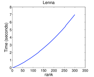
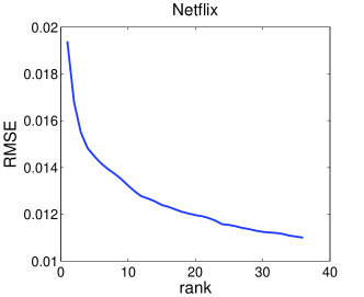
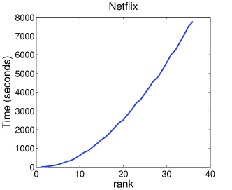
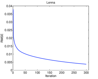
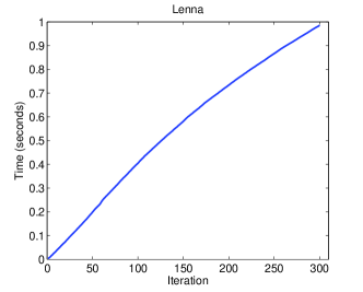
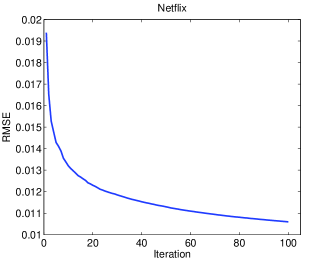
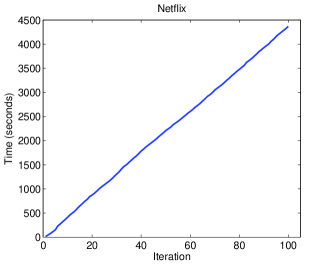
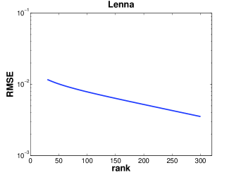
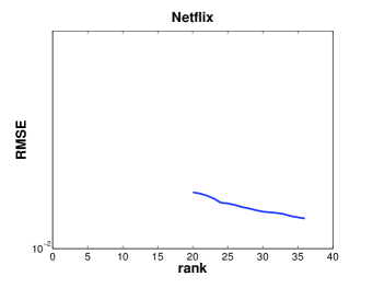
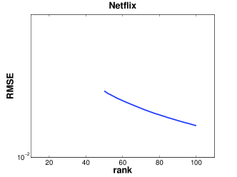
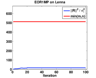
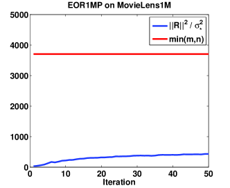
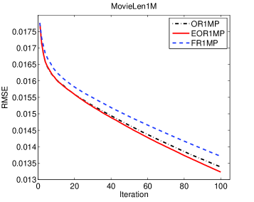
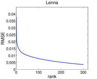
The empirical results for convergence efficiency of our proposed algorithms are reported in Figure 1 and Figure 2. They are based on an image recovery experiment as well as an experiment of completing recommendation dataset, Netflix [22, 4, 5]. The Netflix dataset has 108superscript10810^{8} ratings of 17,770 movies by 480,189 Netflix333http://www.netflixprize.com/ customers. This is a large-scale dataset, and most of the competing methods are not applicable for this dataset. In Figure 1, we present the convergence characteristics of the proposed OR1MP algorithm. As the memory demanded is increasing w.r.t. the iterations, we can only run it for about 40 iterations on the Netflix dataset. The EOR1MP algorithm has no such limitation. The results in Figure 2 show that our EOR1MP algorithm rapidly reduces the approximation error. We also present the same residual curves in logarithmic scale with relatively large number of iterations in Figure 3, which verify the linear convergence property of our algorithms, and this is consistent with our theoretical analysis.
        Refer to caption Refer to caption
        Refer to caption Refer to caption
Fig. 1: Illustration of convergence of the proposed OR1MP algorithm on the Lenna image and the Netflix dataset: the x-axis is the rank, the y-axis is the RMSE (left column), and the running time is measured in seconds (right column).
        Refer to caption Refer to caption
        Refer to caption Refer to caption
Fig. 2: Illustration of convergence of the proposed EOR1MP algorithm on the Lenna image and the Netflix dataset: the x-axis is the rank, the y-axis is the RMSE (left column), and the running time is measured in seconds (right column).
        Refer to caption Refer to caption
        Refer to caption Refer to caption
Fig. 3: Illustration of the linear convergence of different rank-one matrix pursuit algorithms on the Lenna image and the MovieLen1M dataset: the x-axis is the iteration, the y-axis is the RMSE in log scale. The curves in the first row are the results for OR1MP and the curves in the second row are the results for EOR1MP.

In the convergence analysis, we derive the upper bound for the convergence speed of our proposed algorithms. From Theorem 2 and Theorem 9, the convergence speed is controlled by the value of 𝐑kF2/σk,2superscriptsubscriptnormsubscript𝐑𝑘𝐹2superscriptsubscript𝜎𝑘2\|{\bf R}_{k}\|_{F}^{2}/\sigma_{k,*}^{2}, where σk,subscript𝜎𝑘\sigma_{k,*} is the maximum singular value of the residual matrix 𝐑ksubscript𝐑𝑘{\bf R}_{k} in the k𝑘k-th iteration. A smaller value indicates a faster convergence of our algorithms. Though it has a worst case upper bound of 𝐑kF2/σk,2rank(𝐑k)min(m,n)superscriptsubscriptnormsubscript𝐑𝑘𝐹2superscriptsubscript𝜎𝑘2𝑟𝑎𝑛𝑘subscript𝐑𝑘𝑚𝑛\|{\bf R}_{k}\|_{F}^{2}/\sigma_{k,*}^{2}\leq rank({\bf R}_{k})\leq\min(m,n), in the following experiments, we empirically verify that its value is much smaller than the theoretical worst case. Thus the convergence speed of our algorithms is much better than the theoretical worst case. We present the values of 𝐑kF2/σk,2superscriptsubscriptnormsubscript𝐑𝑘𝐹2superscriptsubscript𝜎𝑘2\|{\bf R}_{k}\|_{F}^{2}/\sigma_{k,*}^{2} at different iterations on the Lenna image and the MovieLens1M dataset for both of our algorithms in Figure 4. The results show that the quantity 𝐑kF2/σk,2superscriptsubscriptnormsubscript𝐑𝑘𝐹2superscriptsubscript𝜎𝑘2\|{\bf R}_{k}\|_{F}^{2}/\sigma_{k,*}^{2} is much smaller than min(m,n)𝑚𝑛\min(m,n).

          Refer to caption Refer to caption
          Refer to caption Refer to caption
Fig. 4: Illustration of the values of 𝐑2/σ2superscriptnorm𝐑2subscriptsuperscript𝜎2{\|{\bf R}\|^{2}/{\sigma^{2}_{*}}} at different iterations and the value of min(m,n)𝑚𝑛\min(m,n) on the Lenna image and MovieLens1M for both R1MP and ER1MP algorithms: the x-axis is the iteration number; the y-axis is the value.

In the following experiments, we plot the residual curves over iterations for different rank-one matrix pursuit algorithms, including our OR1MP algorithm, our EOR1MP algorithm and the forward rank-one matrix pursuit algorithm (FR1MP). The evaluations are conducted on the Lenna image and the MovieLens1M dataset, which are given in Figure 5. The results show that among the three algorithms, EOR1MP and OR1MP perform better than the forward pursuit algorithm. It is interesting to note that EOR1MP achieves similar performance as OR1MP, while it demands much less computational cost.
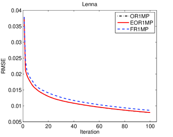
        Refer to caption Refer to caption
Fig. 5: Illustration of convergence speed of different rank-one matrix pursuit algorithms on the Lenna image and the MovieLen1M dataset: the x-axis is the iteration, the y-axis is the RMSE.

7.2 Inexact Top Singular Vectors

We empirically analyze the performance of our algorithms with inexact singular vector computation. In the experiments, we control the total number of iterations in the power method for computing the top singular vector pairs. The numbers of iterations are set as {1,2,5,10,20}1251020\{1,2,5,10,20\}. And we plot the learning curves for OR1MP and EOR1MP algorithms on the MovieLen1M dataset in Figure 6. The results show that the linear convergence speed is preserved for different iteration numbers. However, the results under the same outer iterations depend on the accuracy of the power methods. This verifies our theoretical results. Our empirical results also suggest that in practice we need to run more than 5 iterations in the power method, as the learning curves for 5, 10 and 20 power method iterations are close to each other but are far away from the other two curves, especially for EOR1MP algorithm.
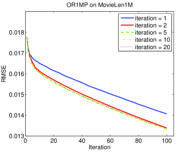
      Refer to caption Refer to caption
Fig. 6: Illustration of convergence property of the proposed algorithms with different iteration numbers in the power method on the MovieLen1M dataset: the x-axis is the outer iteration number; the y-axis is the RMSE.

7.3 Image Recovery

Table 1: Image recovery results measured in terms of the peak signal-to-noise ratio (PSNR).
Data Set SVT SVP SoftImpute LMaFit ADMiRA JS OR1MP EOR1MP
Barbara 26.9635 25.2598 25.6073 25.9589 23.3528 23.5322 26.5314 26.4413
Cameraman 25.6273 25.9444 26.7183 24.8956 26.7645 24.6238 27.8565 27.8283
Clown 28.5644 19.0919 26.9788 27.2748 25.7019 25.2690 28.1963 28.2052
Couple 23.1765 23.7974 26.1033 25.8252 25.6260 24.4100 27.0707 27.0310
Crowd 26.9644 22.2959 25.4135 26.0662 24.0555 18.6562 26.0535 26.0510
Girl 29.4688 27.5461 27.7180 27.4164 27.3640 26.1557 30.0878 30.0565
Goldhill 28.3097 16.1256 27.1516 22.4485 26.5647 25.9706 28.5646 28.5101
Lenna 28.1832 25.4586 26.7022 23.2003 26.2371 24.5056 28.0115 27.9643
Man 27.0223 25.3246 25.7912 25.7417 24.5223 23.3060 26.5829 26.5049
Peppers 25.7202 26.0223 26.8475 27.3663 25.8934 24.0979 28.0781 28.0723
Refer to caption Refer to caption Refer to caption
Fig. 7: The original image and images recovered by different methods on the Lenna image.

In the image recovery experiments, we use the following benchmark test images: Barbara, Cameraman, Clown, Couple, Crowd, Girl, Goldhill, Lenna, Man, Peppers444Images are downloaded from http://www.utdallas.edu/~cxc123730/mh_bcs_spl.html. The size of each image is 512×512512512512\times 512. We randomly exclude 50%percent5050\% of the pixels in the image, and the remaining ones are used as the observations. As the image matrix is not guaranteed to be low rank, we use the rank 50 for the estimation matrix for each experiment. In our OR1MP and EOR1MP algorithms, we stop the algorithms after 150 iterations. The JS algorithm does not explicitly control the rank, thus we fix its number of iterations to 2000. The numerical results in terms of the PSNR are listed in Table 1. We also present the images recovered by different algorithms for Lenna in Figure 7. The results show SVT, our OR1MP and EOR1MP achieve the best numerical performance. However, our algorithm is much better than SVT for Cameraman, Couple, Peppers, but only slightly worse than SVT for Lenna, Barbara and Clown. Besides, our algorithm is much faster and more stable than SVT (SVT easily diverges). For each image, EOR1MP uses around 3.5 seconds, but SVT consumes around 400 seconds. Image recovery needs a relatively higher approximation rank; both GECO and Boost fail to find a good recovery in most cases, so we do not include them in the result tables.

7.4 Recommendation

Table 2: Characteristics of the recommendation datasets.
Data Set # row # column # rating
Jester1 24983 100 106superscript10610^{6}
Jester2 23500 100 106superscript10610^{6}
Jester3 24983 100 666×\times105superscript10510^{5}
MovieLens100k 943 1682 105superscript10510^{5}
MovieLens1M 6040 3706 106superscript10610^{6}
MovieLens10M 69878 10677 107superscript10710^{7}
Table 3: The running time (measured in seconds). Boost fails on MovieLens10M.
Data Set SVP SoftImpute LMaFit Boost JS GECO OR1MP EOR1MP
Jester1 18.3495 161.4941 3.6756 93.9142 29.6751 >104absentsuperscript104>10^{4} 1.8317 0.9924
Jester2 16.8519 152.9600 2.4237 261.7005 28.5228 >104absentsuperscript104>10^{4} 1.6769 0.9082
Jester3 16.5801 1.5450 8.4513 245.7895 12.9441 >103absentsuperscript103>10^{3} 0.9264 0.3415
MovieLens100K 1.3237 128.0658 2.7613 2.8669 2.8583 10.8300 0.0418 0.0358
MovieLens1M 18.9020 59.5600 30.5475 93.9142 13.0972 >104absentsuperscript104>10^{4} 0.8714 0.5397
MovieLens10M >103absentsuperscript103>10^{3} >103absentsuperscript103>10^{3} 154.3760 130.1343 >105absentsuperscript105>10^{5} 23.0513 13.7935
Table 4: Recommendation results measured in terms of the RMSE.
Data Set SVP SoftImpute LMaFit Boost JS GECO OR1MP EOR1MP
Jester1 4.7311 5.1113 4.7623 5.1746 4.4713 4.3680 4.3418 4.3384
Jester2 4.7608 5.1646 4.7500 5.2319 4.5102 4.3967 4.3649 4.3546
Jester3 8.6958 5.4348 9.4275 5.3982 4.6866 5.1790 4.9783 5.0145
MovieLens100K 0.9683 1.0354 1.0238 1.1244 1.0146 1.0243 1.0168 1.0261
MovieLens1M 0.9085 0.8989 0.9232 1.0850 1.0439 0.9290 0.9595 0.9462
MovieLens10M 0.8611 0.8534 0.8971 0.8728 0.8668 0.8621 0.8692

In the following experiments, we compare different matrix completion algorithms using large recommendation datasets: Jester [12] and MovieLens [31]. We use six datasets including: Jester1, Jester2, Jester3, MovieLens100K, MovieLens1M, and MovieLens10M. The statistics of these datasets are given in Table 2. The Jester datasets were collected from a joke recommendation system. They contain anonymous ratings of 100 jokes from the users. The ratings are real values ranging from 10.0010.00-10.00 to +10.0010.00+10.00. The MovieLens datasets were collected from the MovieLens website555http://movielens.umn.edu. They contain anonymous ratings of the movies on this web made by its users. For MovieLens100K and MovieLens1M, there are 5 rating scores (1–5), and for MovieLens10M there are 10 levels of scores with a step size 0.5 in the range of 0.5 to 5. In the following experiments, we randomly split the ratings into training and test sets. Each set contains 50%percent5050\% of the ratings. We compare the running time and the prediction result from different methods. In the experiments, we use 100 iterations for the JS algorithm, and for other algorithms we use the same rank for the estimated matrices; the values of the rank are {10,10,5,10,10,20}10105101020\{10,10,5,10,10,20\} for the six corresponding datasets. We first show the running time of different methods in Table 4. The reconstruction results in terms of the RMSE are given in Table 4. We can observe from the above experiments that our EOR1MP algorithm is the fastest among all competing methods to obtain satisfactory results.

8 Conclusion

In this paper, we propose an efficient and scalable low rank matrix completion algorithm. The key idea is to extend orthogonal matching pursuit method from the vector case to the matrix case. We also propose a novel weight updating rule under this framework to reduce the storage complexity and make it independent of the approximation rank. Our algorithms are computationally inexpensive for each matrix pursuit iteration, and find satisfactory results in a few iterations. Another advantage of our proposed algorithms is they have only one tunable parameter, which is the rank. It is easy to understand and to use by the user. This becomes especially important in large-scale learning problems. In addition, we rigorously show that both algorithms achieve a linear convergence rate, which is significantly better than the previous known results (a sub-linear convergence rate). We also empirically compare the proposed algorithms with state-of-the-art matrix completion algorithms, and our results show that the proposed algorithms are more efficient than competing algorithms while achieving similar or better prediction performance. We plan to generalize our theoretical and empirical analysis to other loss functions in the future.

Appendix A Inverse Matrix Update

In our OR1MP algorithm, we use the least squares solution to update the weights for the rank-one matrix bases. In this step, we need to calculate (𝐌¯𝐤𝐌¯𝐤)1superscriptsubscript¯𝐌𝐤subscript¯𝐌𝐤1({\bf{{\bar{M}}}_{k}}{\bf{{\bar{M}}}_{k}})^{-1}. To directly compute this inverse is computationally expensive, as the matrix 𝐌¯𝐤subscript¯𝐌𝐤{\bf{{\bar{M}}}_{k}} has large row size. We implement this efficiently using an incremental method. As

𝐌¯𝐤T𝐌¯𝐤=[𝐌¯𝐤𝟏,𝐦˙k]T[𝐌¯𝐤𝟏,𝐦˙k],superscriptsubscript¯𝐌𝐤𝑇subscript¯𝐌𝐤superscriptsubscript¯𝐌𝐤1subscript˙𝐦𝑘𝑇subscript¯𝐌𝐤1subscript˙𝐦𝑘{\bf{{\bar{M}}}_{k}}^{T}{\bf{{\bar{M}}}_{k}}=[{\bf{{\bar{M}}}_{k-1}},\dot{\bf m}_{k}]^{T}[{\bf{{\bar{M}}}_{k-1}},\dot{\bf m}_{k}],

its inverse can be written in block matrix form

(𝐌¯𝐤T𝐌¯𝐤)1=[𝐌¯𝐤𝟏T𝐌¯𝐤𝟏𝐌¯𝐤𝟏T𝐦˙k𝐦˙kT𝐌¯𝐤𝟏T𝐦˙kT𝐦˙k]1.superscriptsuperscriptsubscript¯𝐌𝐤𝑇subscript¯𝐌𝐤1superscriptmatrixsuperscriptsubscript¯𝐌𝐤1𝑇subscript¯𝐌𝐤1superscriptsubscript¯𝐌𝐤1𝑇subscript˙𝐦𝑘subscriptsuperscript˙𝐦𝑇𝑘superscriptsubscript¯𝐌𝐤1𝑇subscriptsuperscript˙𝐦𝑇𝑘subscript˙𝐦𝑘1({\bf{{\bar{M}}}_{k}}^{T}{\bf{{\bar{M}}}_{k}})^{-1}=\begin{bmatrix}{\bf{{\bar{M}}}_{k-1}}^{T}{\bf{{\bar{M}}}_{k-1}}&{\bf{{\bar{M}}}_{k-1}}^{T}\dot{\bf m}_{k}\\ \dot{\bf m}^{T}_{k}{\bf{{\bar{M}}}_{k-1}}^{T}&\dot{\bf m}^{T}_{k}\dot{\bf m}_{k}\end{bmatrix}^{-1}.\\

Then it is calculated by blockwise inversion as

[𝐀+d𝐀𝐛𝐛T𝐀d𝐀𝐛d𝐛T𝐀d]matrix𝐀𝑑superscript𝐀𝐛𝐛𝑇𝐀𝑑𝐀𝐛𝑑superscript𝐛𝑇𝐀𝑑missing-subexpression\begin{array}[]{lc}\begin{bmatrix}{\bf A}+d{\bf A}{\bf b}{\bf b}^{T}{\bf A}&-d{\bf A}{\bf b}\\ -d{\bf b}^{T}{\bf A}&{d}\end{bmatrix}\end{array}

where 𝐀=(𝐌¯𝐤𝟏T𝐌¯𝐤𝟏)1𝐀superscriptsuperscriptsubscript¯𝐌𝐤1𝑇subscript¯𝐌𝐤11{\bf A}=({\bf{{\bar{M}}}_{k-1}}^{T}{\bf{{\bar{M}}}_{k-1}})^{-1} is the corresponding inverse matrix in the last step, 𝐛=𝐌¯𝐤𝟏T𝐦˙k𝐛superscriptsubscript¯𝐌𝐤1𝑇subscript˙𝐦𝑘{\bf b}={\bf{{\bar{M}}}_{k-1}}^{T}\dot{\bf m}_{k} is a vector with |Ω|Ω|\Omega| elements, and d=(𝐛T𝐛𝐛T𝐀𝐛)1=1/(𝐛T𝐛𝐛T𝐀𝐛)𝑑superscriptsuperscript𝐛𝑇𝐛superscript𝐛𝑇𝐀𝐛11superscript𝐛𝑇𝐛superscript𝐛𝑇𝐀𝐛d=({\bf b}^{T}{\bf b}-{\bf b}^{T}{\bf A}{\bf b})^{-1}=1/({\bf b}^{T}{\bf b}-{\bf b}^{T}{\bf A}{\bf b}) is a scalar.

𝐌¯𝐤T𝐲˙superscriptsubscript¯𝐌𝐤𝑇˙𝐲{\bf{{\bar{M}}}_{k}}^{T}{\dot{\bf y}} is also calculated incrementally by [𝐌¯𝐤𝟏T𝐲˙,𝐦˙kT𝐲˙]superscriptsubscript¯𝐌𝐤1𝑇˙𝐲subscriptsuperscript˙𝐦𝑇𝑘˙𝐲[{\bf{{\bar{M}}}_{k-1}}^{T}{\dot{\bf y}},\dot{\bf m}^{T}_{k}{\dot{\bf y}}], as 𝐲˙˙𝐲\dot{\bf y} is fixed.

References

  • [1] A. Argyriou, T. Evgeniou, and M. Pontil, Convex multi-task feature learning, Machine Learning, 73 (2008), pp. 243–272.
  • [2] F. Bach, Consistency of trace norm minimization, Journal of Machine Learning Research, 9 (2008), pp. 1019–1048.
  • [3] L. Balzano, R. Nowak, and B. Recht, Online identification and tracking of subspaces from highly incomplete information, in Proceedings of the Allerton Conference on Communication, Control and Computing, 2010.
  • [4] R. Bell and Y. Koren, Lessons from the netflix prize challenge, SIGKDD Explorations, 9 (2007).
  • [5] J. Bennett and S. Lanning, The netflix prize, in Proceedings of KDD Cup and Workshop, 2007.
  • [6] J.-F. Cai, E. J. Candès, and Z. Shen, A singular value thresholding algorithm for matrix completion, SIAM Journal on Optimization, 20 (2010), pp. 1956–1982.
  • [7] E. J. Candès and B. Recht, Exact matrix completion via convex optimization, Foundations of Computational Mathematics, 9 (2009), pp. 717–772.
  • [8] R. A. DeVore and V. N. Temlyakov, Some remarks on greedy algorithms, Advances in computational Mathematics, 5 (1996), pp. 173–187.
  • [9] M. Dudík, Z. Harchaoui, and J. Malick, Lifted coordinate descent for learning with trace-norm regularization, in Proceedings of the 15th International Conference on Artificial Intelligence and Statistics (AISTATS), 2012.
  • [10] M. Frank and P. Wolfe, An algorithm for quadratic programming, Naval Research Logistics Quarterly, 3 (1956), pp. 95–110.
  • [11] J. H. Friedman, T. Hastie, and R. Tibshirani, Regularization paths for generalized linear models via coordinate descent, Journal of Statistical Software, 33 (2010), pp. 1–22.
  • [12] K. Goldberg, T. Roeder, D. Gupta, and C. Perkins, Eigentaste: A constant time collaborative filtering algorithm, Information Retrieval, 4 (2001), pp. 133–151.
  • [13] G. H. Golub and C. F. V. Loan, Matrix computations (3rd ed.), The Johns Hopkins University Press, 1996.
  • [14] T. Hastie, R. Tibshirani, and J. H. Friedman, The elements of statistical learning: data mining, inference, and prediction, New York: Springer-Verlag, 2009.
  • [15] E. Hazan, Sparse approximate solutions to semidefinite programs, in Proceedings of the 8th Latin American conference on Theoretical informatics, 2008.
  • [16] Q. Huynh-Thu and M. Ghanbari, Scope of validity of psnr in image/video quality assessment, Electronics Letters, 44 (2008), pp. 800–801.
  • [17] M. Jaggi and M. Sulovský, A simple algorithm for nuclear norm regularized problems, in Proceedings of the 27th International Conference on Machine Learning (ICML), 2010, pp. 471–478.
  • [18] P. Jain, R. Meka, and I. S. Dhillon, Guaranteed rank minimization via singular value projection, in Advances in Neural Information Processing Systems (NIPS) 22, 2010, pp. 937–945.
  • [19] P. Jain, P. Netrapalli, and S. Sanghavi, Low-rank matrix completion using alternating minimization, in Proceedings of the 45th Annual ACM Symposium on Symposium on Theory of Computing (STOC), 2013, pp. 665–674.
  • [20] S. Ji and J. Ye, An accelerated gradient method for trace norm minimization, in Proceedings of the 26th International Conference on Machine Learning (ICML), 2009, pp. 457–464.
  • [21] R. Keshavan and S. Oh, Optspace: A gradient descent algorithm on grassmann manifold for matrix completion, http://arxiv.org/abs/0910.5260, (2009).
  • [22] Y. Koren, Factorization meets the neighborhood: a multifaceted collaborative filtering model, in Proceedings of the 14th ACM SIGKDD international conference on Knowledge discovery and data mining (KDD), 2008.
  • [23] Y. Koren, R. Bell, and C. Volinsky, Matrix factorization techniques for recommender systems, Computer, (2009).
  • [24] M.-J. Lai, Y. Xu, and W. Yin, Improved iteratively reweighted least squares for unconstrained smoothed qsubscript𝑞\ell_{q} minimization,, SIAM Journal on Numerical Analysis, (2012).
  • [25] K. Lee and Y. Bresler, Admira: atomic decomposition for minimum rank approximation, IEEE Transactions on Information Theory, 56 (2010), pp. 4402–4416.
  • [26] E. Liu and T. N. Temlyakov, The orthogonal super greedy algorithm and applications in compressed sensing, IEEE Transactions on Information Theory, 58 (2012), pp. 2040–2047.
  • [27] Y.-J. Liu, D. Sun, and K.-C. Toh, An implementable proximal point algorithmic framework for nuclear norm minimization, Mathematical Programming, 133 (2012), pp. 399–436.
  • [28] Z. Lu and Y. Zhang, Penalty decomposition methods for rank minimization, http://arxiv.org/abs/0910.5260, (2010).
  • [29] S. Ma, D. Goldfarb, and L. Chen, Fixed point and bregman iterative methods for matrix rank minimization, Mathematical Programming, 128 (2011), pp. 321–353.
  • [30] R. Mazumder, T. Hastie, and R. Tibshirani, Spectral regularization algorithms for learning large incomplete matrices, Journal of Machine Learning Research, 99 (2010), pp. 2287–2322.
  • [31] B. N. Miller, I. Albert, S. K. Lam, J. A. Konstan, and J. Riedl, Movielens unplugged: experiences with an occasionally connected recommender system, in Proceedings of the 8th international conference on Intelligent user interfaces, 2003, pp. 263–266.
  • [32] B. Mishra, G. Meyer, F. Bach, and R. Sepulchre, Low-rank optimization with trace norm penalty, http://arxiv.org/abs/1112.2318, (2011).
  • [33] D. Needell and J. A. Tropp, Cosamp: iterative signal recovery from incomplete and inaccurate samples, Communications of the ACM, 53 (2010), pp. 93–100.
  • [34] S. Negahban and M. Wainwright, Estimation of (near) low-rank matrices with noise and high-dimensional scaling, in Proceedings of the 27th International Conference on Machine Learning (ICML), 2010.
  • [35] Y. C. Pati, R. Rezaiifar, Y. C. P. R. Rezaiifar, and P. S. Krishnaprasad, Orthogonal matching pursuit: Recursive function approximation with applications to wavelet decomposition, in Proceedings of the 27th Annual Asilomar Conference on Signals, Systems, and Computers, 1993, pp. 40–44.
  • [36] B. Recht, M. Fazel, and P. A. Parrilo, Guaranteed minimum-rank solutions of linear matrix equations via nuclear norm minimization, SIAM Review, 52 (2010), pp. 471–501.
  • [37] B. Recht and C. Ré, Parallel stochastic gradient algorithms for large-scale matrix completion, Mathematical Programming Computation, 5 (2013), pp. 201–226.
  • [38] S. Shalev-Shwartz, A. Gonen, and O. Shamir, Large-scale convex minimization with a low-rank constraint, in Proceedings of the 28th International Conference on Machine Learning (ICML), 2011, pp. 329–336.
  • [39] S. Shalev-Shwartz and A. Tewari, Stochastic methods for l1 regularized loss minimization, in Proceedings of the 26th International Conference on Machine Learning (ICML), 2009, pp. 929–936.
  • [40] N. Srebro, J. Rennie, and T. Jaakkola, Maximum margin matrix factorizations, in Advances in Neural Information Processing Systems (NIPS) 17, 2005.
  • [41] V. N. Temlyakov, Greedy approximation, Acta Numerica, 17 (2008), pp. 235–409.
  • [42] A. Tewari, P. Ravikumar, and I. S. Dhillon, Greedy algorithms for structurally constrained high dimensional problems, in Advances in Neural Information Processing Systems (NIPS) 23, 2011.
  • [43] R. Tibshirani, Regression shrinkage and selection via the lasso, Journal of the Royal Statistical Society, Series B, 58 (1994), pp. 267–288.
  • [44] K.-C. Toh and S. Yun, An accelerated proximal gradient algorithm for nuclear norm regularized least squares problems, Pacific Journal of Optimization, 6 (2010), pp. 615 – 640.
  • [45] J. A. Tropp, Greed is good: algorithmic results for sparse approximation, IEEE Trans. Inform. Theory, 50 (2004), pp. 2231–2242.
  • [46] Z. Wen, W. Yin, and Y. Zhang, Low-rank factorization model for matrix completion by a non-linear successive over-relaxation algorithm, Rice CAAM Tech Report 10-07, University of Rice, 2010.
  • [47] T. T. Wu and K. Lange, Coordinate descent algorithms for lasso penalized regression, Annals of Applied Statistics, 2 (2008), pp. 224–244.
  • [48] S. Yun and K.-C. Toh, A coordinate gradient descent method for l1-regularized convex minimization, Computational Optimization and Applications, (2011).
  • [49] X. Zhang, Y. Yu, and D. Schuurmans, Accelerated training for matrix-norm regularization: A boosting approach, in Advances in Neural Information Processing Systems (NIPS) 24, 2012.