Spectrum of the totally asymmetric simple exclusion process on a periodic lattice - first excited states

Abstract

We consider the spectrum of the totally asymmetric simple exclusion process on a periodic lattice of $L$ sites. The first eigenstates have an eigenvalue with real part scaling as $L^{-3/2}$ for large $L$ with finite density of particles. Bethe ansatz shows that these eigenstates are characterized by four finite sets of positive half-integers, or equivalently by two integer partitions. Each corresponding eigenvalue is found to be equal to the value at its saddle point of a function indexed by the four sets. Our derivation of the large $L$ asymptotics relies on a version of the Euler-Maclaurin formula with square root singularities at both ends of the summation range.

PACS numbers: 02.30.Ik 02.50.Ga 05.40.-a 05.60.Cd

Keywords: TASEP, complex spectrum, non-Hermitian operator

1 Introduction

The one dimensional totally asymmetric simple exclusion process (TASEP) [1, 2, 3, 4, 5] is a Markov process featuring classical hard-core particles moving in the same direction on a lattice. It has been much studied in the last 20 years as a simple example of a genuine non-equilibrium process with transition rates breaking detailed balance. Another interest in TASEP, as well as its generalization ASEP where particles hop in both direction with different rates, comes from a mapping to a microscopic model of a growing interface. At large scales, the dynamics of the interface is described by a very singular [6] nonlinear stochastic partial differential equation called the Kardar-Parisi-Zhang (KPZ) equation [7, 8, 9, 10, 11].

Models in the one dimensional KPZ universality class are characterized by a dynamical exponent $z=3/2$, which means that the relaxation time grows as $L^{3/2}$ for large system size $L$. The relaxation time is equal to the inverse of the gap between the stationary eigenvalue of the time evolution operator and the eigenvalue of the first excited state. The large $L$ asymptotics of the gap has been computed exactly for periodic TASEP [12, 13, 14, 15, 16] and ASEP [17], as well as for TASEP [18, 19] and ASEP [20, 21] on an open interval connected to reservoirs of particles, and also for generalizations of ASEP with several species of particles [22, 23] and with extended particles [24]. The gap of more general reaction diffusion processes has also been studied [25].

Many exact results have also been obtained for the fluctuations and large deviations [26, 27] of exclusion processes observed at large scales. In the stationary state, with a time of observation much larger than the relaxation time, explicit formulas have been derived for the large deviation function of the current of particles for periodic TASEP [28, 29] and ASEP [30, 31, 32, 33, 34, 35], and also for TASEP [36] and ASEP [37, 38, 39, 40] with open boundaries or with several species of particles [41, 42]. These large deviation functions, which are in general non-Gaussian, verify a Gallavotti-Cohen symmetry relation [43, 44]. On the other hand, the transient regime, with times of observation much smaller than the relaxation time, has been studied a lot in the context of height fluctuations for KPZ universality class [45, 46, 47, 48]. The probability distribution of the current fluctuations in TASEP [49, 50] and ASEP [51, 52, 53] have been found to be related to known distributions from random matrix theory, see also [54, 55] for related results for the problem of a directed polymer in a random medium, which also belong to KPZ universality class.

A clear link is still missing between the results for the current fluctuations obtained in the stationary and in the transient regime, see however [56, 57, 58, 59] for studies in the crossover regime, with an observation time of the order of the relaxation time. An exact calculation of the crossover behaviour would presumably require a summation over the corresponding eigenstates, and thus the knowledge of all eigenvectors and eigenvalues. This motivates further study of the spectrum beyond the gap. In [60], the bulk of the spectrum of TASEP was studied, with eigenvalues scaling proportionally to $L$ for large system size $L$. We consider here the first eigenvalues, which scale as $L^{-3/2}$ like the gap.

Explicit calculations for exclusion processes are made possible by the use of Bethe ansatz, which was initially introduced to diagonalize the Hamiltonian of Heisenberg spin chain. Exclusion processes possess the same kind of mathematical structures as quantum integrable models, although they are models of classical particles. In particular, one can define [3] for them a family of transfer matrices which commute with each other as a consequence of Yang-Baxter equation. Several aspects of the integrability of exclusion processes have been studied, for periodic systems [61, 62, 63, 64], with open boundaries [65, 66, 67], on the infinite line [68, 69, 70], and with more general hopping rules [71].

We study in this paper the structure of eigenvalues of periodic TASEP for higher excited states beyond the gap. We use Bethe ansatz in section 2 to write the eigenvalues for finite number of particles on a finite lattice. The large $L$ asymptotics performed in section 3 relies on a version of the Euler-Maclaurin formula with square root singularities at both ends of the summation range (72), which is somewhat simpler than the previous derivations in the case of the gap. Section 4 is devoted to the study of a function in terms of which the eigenvalues are expressed. A numerical study of the first eigenvalues is made in section 5, as well as some asymptotics when one goes deeper into the spectrum.

2 First excited states

2.1 The Markov matrix

We consider the one-dimensional TASEP on a periodic lattice with $L$ sites. The $N$ particles of the system, $0<N<L$, move in continuous time by hopping from site to site in the forward direction. A particle can only hop if the destination site is empty, so that at any time each site is either empty or occupied by exactly one particle. Particles hop at a distance $1$ on the lattice, with hopping rate equal to $1$: in a small time interval $dt$, each particle moves with probability $dt$ if the site next to it in the forward direction is empty. The definition of the model is summarized in figure 1.

The time evolution is encoded in a Markov matrix $M$, whose non-diagonal entries encode the transition rates between configurations: for $\mathcal{C}\neq\mathcal{C}^{\prime}$, the matrix element $M(\mathcal{C}^{\prime},\mathcal{C})\geq 0$ is the rate at which the system goes from configuration $\mathcal{C}$ to configuration $\mathcal{C}^{\prime}$. This rate is either $1$ if $\mathcal{C}^{\prime}$ can be obtained from $\mathcal{C}$ by moving one and only one particle, and $0$ otherwise. The diagonal entries $M(\mathcal{C},\mathcal{C})$ are equal to minus the total exit rate from configuration $\mathcal{C}$.

Since the dynamics of TASEP breaks detailed balance, the eigenvalues $E$ of $M$ are in general complex numbers. They verify $\mathrm{Re}\,E<0$ except for the stationary state which has $E=0$. The relaxation toward the stationary state is governed by the eigenstate whose eigenvalue has the smallest real part, stationary eigenvalue excepted. This minimal value of $|\mathrm{Re}\,E|$ is called the gap, and is equal to the inverse of the relaxation time. It was shown in [12, 13, 14, 15, 16] that in the thermodynamic limit $L,N\to\infty$ with density $\rho=N/L$ fixed, the gap scales as $L^{-3/2}$.

Figure 1: The totally asymmetric simple exclusion process (TASEP) on a one-dimensional lattice with periodic boundary conditions. Particles hop only in the clockwise direction.

2.2 The transfer matrix

The quantum integrability of TASEP can be understood in terms of a family $t(\lambda)$ of commuting transfer matrices, $t(\lambda)t(\mu)=t(\mu)t(\lambda)$ for any $\lambda$ and $\mu$, see e.g. [3]. This commutation relation is a consequence of Yang-Baxter equation. The parameter $\lambda$ of the transfer matrix is usually called the spectral parameter.

For $\lambda\in[0,1]$, the transfer matrix is the Markov matrix of a process in discrete time with parallel update and long range hopping, with transition probabilities depending on $\lambda$ as a geometric progression with the total distance travelled [63]. We show in section 3.3 that the real part of the first eigenvalues of $t(\lambda)-\mbox{{\small 1}$\!\!$1}$ scale as $L^{-3/2}$ for $\lambda\in[0,1]$: the relaxation time of the model with long range hopping described by $t(\lambda)$ grows as $L^{3/2}$ similarly to TASEP.

The Markov matrix $M$ of TASEP is equal to $M=t^{\prime}(0)t^{-1}(0)$. One can also define from the transfer matrix generalized ”Hamiltonians” $F_{k}=[\partial_{\lambda}^{k}\log t(\lambda)]_{|\lambda\to 0}$ which commute with $M$ and contain only interactions on at most $k+1$ neighbouring sites [63, 64]. The operators $F_{k}$, $k\geq 2$ are in general not Markovian as some of their non-diagonal entries are negative.

2.3 Eigenvalues from Bethe ansatz

Each eigenvector $|\Psi\rangle$ of the Markov matrix $M$, and more generally of the transfer matrix $t(\lambda)$, can be expressed in terms of $N$ Bethe roots $y_{1}$, …, $y_{N}$ (that depend on the eigenstate) as

$$\Psi(x_{1},\ldots,x_{N})=\langle x_{1},\ldots,x_{N}|\Psi\rangle=\det\Big{[}\Big{(}\frac{y_{k}}{y_{j}}\Big{)}^{N-j}(1-y_{k})^{x_{j}}\Big{]}_{j,k=1,\ldots,N}\;.$$ (1)

The corresponding eigenvalue $E$ of $M$ is equal to

$$E=\sum_{j=1}^{N}\frac{y_{j}}{1-y_{j}}\;,$$ (2)

and the Bethe roots must be solution of the Bethe equations

$$(1-y_{j})^{L}=(-1)^{N-1}\prod_{k=1}^{N}\frac{y_{j}}{y_{k}}\;.$$ (3)

The stationary eigenstate corresponds to $y_{j}=0$ for all $j$, for which the right hand side of Bethe equations is not well defined. This solution can in fact be understood by the introduction of a small twist $\gamma>0$, see e.g. [60], and by taking the limit $\gamma\to 0$. Apart from this peculiarity, it is believed that (2), (3) gives all the other eigenvalues of $M$, although a rigorous proof is still missing (see however [72] for a discrete time case).

We define the parameter

$$b=\frac{1}{L}\sum_{j=1}^{N}\log y_{j}\;.$$ (4)

Taking the power $1/L$ of the Bethe equations (3), it follows that there must exist numbers $k_{j}$, integers if $N$ is odd, half-integers if $N$ is even, such that

$$\frac{1-y_{j}}{y_{j}^{\rho}}=\rme^{\frac{2\rmi\pi k_{j}}{L}-b}\;,$$ (5)

where $\rho=N/L$ is the density of particles. By analogy with the case of undistinguishable free particles (see e.g. [60], Appendix D), the numbers $k_{j}$ must be distinct modulo $L$. They can be ordered as $0<k_{1}<\ldots<k_{N}\leq L$ so that each eigenstate is counted only once.

It turns out that the function $g:y\mapsto(1-y)/y^{\rho}$ is a bijection of the complex plane (minus the cut $\mathbb{R}^{-}$ and its image by $g$, see A). Eq (5) can then be solved for $y_{j}$ in terms of the reciprocal function $g^{-1}$. In the following, we use the function $\psi=\log g^{-1}$ instead of $g^{-1}$. It can be defined as the solution of the implicit equation

$$\rme^{\psi(z)}+z\,\rme^{\rho\psi(z)}=1\;$$ (6)

such that $-\pi<\mathrm{Im}\,\psi(z)<\pi$. In particular, at half-filling $\rho=1/2$, one has $\psi(z)=-2\log(z/2+\sqrt{1+z^{2}/4})$, while $\psi(z)\to\log(1-z)$ for $\rho\to 0$ and $\psi(z)\to-\log(1+z)$ for $\rho\to 1$. Some properties of the function $\psi$ are discussed in A for general $\rho$. A plot of contour lines of $\psi$ is given in figure 2.

Writing

$$y_{j}=\exp\Big{(}\psi\Big{(}\rme^{\frac{2\rmi\pi k_{j}}{L}-b}\Big{)}\Big{)}\;,$$ (7)

we can finally express the eigenvalues of the Markov matrix in terms of the function $\psi$ as

$$E=\sum_{j=1}^{N}\Big{(}\exp\Big{[}-\psi\Big{(}\rme^{\frac{2\rmi\pi k_{j}}{L}-b}\Big{)}\Big{]}-1\Big{)}^{-1}\;,$$ (8)

where the parameter $b$ is solution of

$$b=\frac{1}{L}\sum_{j=1}^{N}\psi\Big{(}\rme^{\frac{2\rmi\pi k_{j}}{L}-b}\Big{)}\;.$$ (9)

The translation operator commutes with the Markov matrix. From (1), its eigenvalue $\rme^{2\rmi\pi P/L}$, $P\in\mathbb{Z}$ for the eigenstate with Bethe roots $y_{j}$ is $\rme^{2\rmi\pi P/L}=\prod_{j=1}^{N}(1-y_{j})$. Using (5) and (4), one has $\rme^{2\rmi\pi P/L}=\prod_{j=1}^{N}\rme^{2\rmi\pi k_{j}/L}$, thus

$$P=\sum_{j=1}^{N}k_{j}\quad\mathrm{mod}\,L\;.$$ (10)

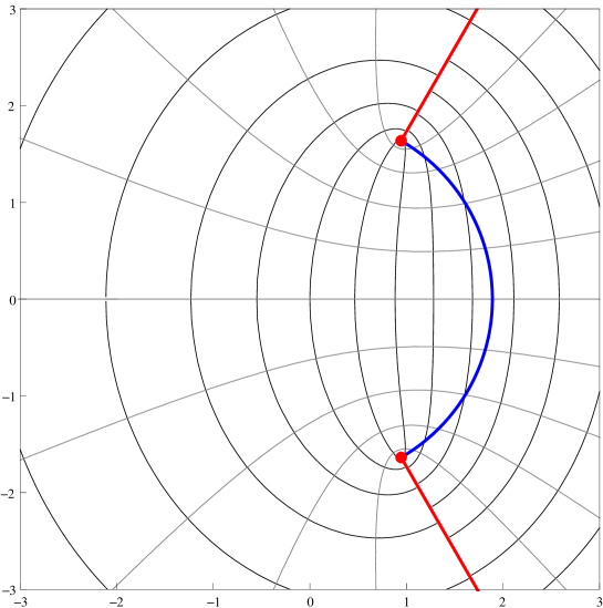
Figure 2: Contour lines of the function $\psi$, defined implicitely in (6), for $\rho=1/3$. The black curves correspond to the $z$ of the complex plane such that $\mathrm{Re}\,\psi(z)=2,\,1.5,\,1,\,\ldots,\,-4$ from left to right. The gray curves correspond to the $z$ such that $\mathrm{Im}\,\psi(z)=-\frac{4\pi}{5},\,-\frac{3\pi}{5},\,\ldots,\,\frac{4\pi}{5}$ from up to down. The two thick, red lines are the branch cuts of $\psi$. The thick, blue curve that links the two branch points is the set of the $z=\rme^{2\rmi\pi u-b_{0}}$ for $-\frac{\rho}{2}<u<\frac{\rho}{2}$ with $b_{0}$ defined in (19): this is the contour used in the integrals of equations (24) and (32).

2.4 Lowest eigenvalues

The stationary state $E=0$ corresponds in principle to the choice $k_{j}=k_{j}^{(0)}$, with

$$k_{j}^{(0)}=j-\frac{N+1}{2}\quad\mathrm{mod}\;L\;.$$ (11)

Numerical studies seem to indicate that for this choice, (9) does not have any finite solution for $b$. This problem can be avoided if one introduces a small twist, as mentioned in section 2.3. For all the other choices of the $k_{j}$’s, however, (9) seems to have a unique solution for $b$.
The first excitations above the stationary state (corresponding to eigenvalues with real part closest to $0$) correspond to sets of $k_{j}$’s obtained from $k_{j}^{(0)}$ by moving a finite number of $k_{j}^{(0)}$ of a finite distance for large $L$, with the density of particles $\rho=N/L$ taken fixed. Since the $k_{j}^{(0)}$’s completely fill the interval $[-\rho L/2,\rho L/2]$, one can only move $k_{j}^{(0)}$’s that are close to $\pm\rho L/2$. In particular, the first excited state (or gap) has a doubly degenerate real part: the corresponding eigenvalues $E_{1}^{\pm}$, which are complex conjugate of each other, correspond to $k_{j}=k_{j}^{(0)}$, $j=1,\ldots,N-1$, $k_{N}=(N+1)/2$ and to $k_{j}=k_{j}^{(0)}$, $j=2,\ldots,N$, $k_{1}=-(N+1)/2$, see figure 3.

Figure 3: Choices of the numbers $k_{j}$, $j=1,\ldots,N$ characterizing some eigenstates. The gray squares represent the $k_{j}$’s chosen. The upper line corresponds to the choice for the stationary state (11). The second and third lines are the two possible choices for the gap. The last line corresponds to a generic eigenstate close to the stationary state, defined by sets $A_{0}^{-}=\{\frac{1}{2},\frac{5}{2}\}$, $A^{-}=\{\frac{1}{2},\frac{7}{2}\}$, $A_{0}^{+}=\{\frac{1}{2},\frac{5}{2},\frac{7}{2}\}$, $A^{+}=\{\frac{3}{2},\frac{5}{2},\frac{9}{2}\}$ of cardinals $m_{-}=|A_{0}^{-}|=|A^{-}|=2$ and $m_{+}=|A_{0}^{+}|=|A^{+}|=3$.

More generally, any excited state close to the stationary state can be defined by four finite sets of half integers describing which $k_{j}$’s are removed from both ends and where they are placed: the $k_{j}$’s removed are equal to $\pm(\rho L/2-a)$, $a\in A_{0}^{\pm}$, and they are placed at $\pm(\rho L/2+a)$, $a\in A^{\pm}$, with

$$m_{\pm}=|A_{0}^{\pm}|=|A^{\pm}|\qquad A_{0}^{\pm},A^{\pm}\subset\mathbb{N}+\frac{1}{2}\;.$$ (12)

Then, for any function $f$, one can write

$$\sum_{j=1}^{N}f\Big{(}\frac{k_{j}}{L}\Big{)}=\sum_{j=1}^{N}f\Big{(}\frac{k_{j}^{(0)}}{L}\Big{)}+\sum_{a\in A^{+}}f\Big{(}\frac{\rho}{2}+\frac{a}{L}\Big{)}+\sum_{a\in A^{-}}f\Big{(}-\frac{\rho}{2}-\frac{a}{L}\Big{)}$$ (13)

$$\hskip 133.72795pt-\sum_{a\in A_{0}^{+}}f\Big{(}\frac{\rho}{2}-\frac{a}{L}\Big{)}-\sum_{a\in A_{0}^{-}}f\Big{(}-\frac{\rho}{2}+\frac{a}{L}\Big{)}\;.$$

In particular, taking $f$ equal to the identity function and using (12), the total momentum (10) rewrites

$$P=\sum_{a\in A_{0}^{+}}a+\sum_{a\in A^{+}}a-\sum_{a\in A_{0}^{-}}a-\sum_{a\in A^{-}}a\;.$$ (14)

We use again (13) in section 3 to extract the large $L$ asymptotics of $b$ and $E$ for the first excited states. A crucial point will be that both ends of the summation over $j$ in the right hand side of (13) applied to (8), (9) correspond to branch points of the function $\psi$.

2.5 Reformulation in terms of partitions of integers

We define an index $Q$ equal to

$$Q=Q_{+}+Q_{-}\quad\mathrm{with}\quad Q_{\pm}=\sum_{a\in A_{0}^{\pm}}a+\sum_{a\in A^{\pm}}a\;.$$ (15)

The index $Q$ is useful in order to generate the first eigenvalues by increasing real part, see table 1 and figure 8.

We show in this section that the number $\Omega(Q)$ of eigenstates with a given value of $Q$ is equal to

$$\Omega(Q)=\sum_{q=0}^{Q}p(q)p(Q-q)\underset{Q\to\infty}{\simeq}\frac{3^{1/4}}{12Q^{5/4}}\,\rme^{2\pi\sqrt{Q/3}}\;,$$ (16)

where $p(n)$ is the number of ways to partition $n$ as an unordered sum of positive integers. The numbers $\Omega(Q)$, $Q\in\mathbb{N}$ form the sequence A000712 of [73]. The large $Q$ behaviour follows from Hardy-Ramanujan asymptotics of $p(n)$ [74].

In order to prove (16), we construct a bijection between unordered partitions of $q$, and the ensemble of all possible choices for sets of positive half-integers $A_{0}$ and $A$ with same cardinal and verifying $q=\sum_{a\in A_{0}}a+\sum_{a\in A}a$. Calling $m$ the cardinal of $A_{0}$ and $A$, and respectively $a_{j}^{(0)}$ and $a_{j}$ the elements of $A_{0}$ and $A$ ordered from largest to smallest, one has

$$q=-m^{2}+\sum_{j=1}^{m}(a_{j}^{(0)}+j-\mbox{\small$\frac{1}{2}$})+\sum_{j=1}^{m}(a_{j}+j-\mbox{\small$\frac{1}{2}$})\;.$$ (17)

The numbers $a_{j}^{(0)}+j-\frac{1}{2}$ and $a_{j}+j-\frac{1}{2}$ are integers larger or equal to $m$, non-increasing as $j$ increases. We define two partitions $\ell$ and $\overline{\ell}$ by $\ell_{j}=a_{j}^{(0)}+j-\frac{1}{2}$ and $\overline{\ell}_{j}=a_{j}+j-\frac{1}{2}$ for $1\leq j\leq m$ and $\ell_{j},\overline{\ell}_{j}\leq m$ for $j>m$. Adding the requirement that $\overline{\ell}$ is the conjugate partition of $\ell$ (the Ferrers diagram of $\overline{\ell}$ is obtained from the one of $\ell$ by exchanging the rows and the columns), this defines a unique pair $(\ell,\overline{\ell})$ of partitions, see figure 4. The number $q$ is then partitioned as $q=\ell_{1}+\ldots+\ell_{n}=\overline{\ell}_{1}+\ldots+\overline{\ell}_{\overline{n}}$ with $n=\overline{\ell}_{1}$ and $\overline{n}=\ell_{1}$. The cardinal $m$ of $A_{0}$ and $A$ corresponds to the size of the Durfee square of the partition (largest square that can fit in the Ferrers diagram).

Figure 4: Ferrers diagram associated to a partition $\ell$ of the integer $q=20$. Two sets of positive half-integers $A_{0}=\{a_{1}^{(0)},\ldots,a_{m}^{(0)}\}$ and $A=\{a_{1},\ldots,a_{m}\}$ are constructed from it, with $a_{j}^{(0)}$ equal to the number of filled dots in the $j$-th row, and $a_{j}$ equal to the number of filled dots in the $j$-th column. Half-filled dots count for $\frac{1}{2}$. The $m\times m$ Durfee square of the Ferrers diagram is represented in the picture.

In the rest of the article, we write everything in terms of the sets $A_{0}^{\pm}$, $A^{\pm}$. The translation to integer partitions $\ell^{\pm}$ and their conjugates $\overline{\ell^{\pm}}$ can be done with the following formulas, valid for an arbitrary function $f$:

$$\sum_{a\in A_{0}^{+}}f(a)=\sum_{j=1}^{m_{+}}f(\ell_{j}^{+}-j+\mbox{\small$\frac{1}{2}$})\qquad\sum_{a\in A^{+}}f(a)=\sum_{j=1}^{m_{+}}f(\overline{\ell^{+}_{j}}-j+\mbox{\small$\frac{1}{2}$})$$ (18)

$$\sum_{a\in A_{0}^{-}}f(a)=\sum_{j=1}^{m_{-}}f(\ell_{j}^{-}-j+\mbox{\small$\frac{1}{2}$})\qquad\sum_{a\in A^{-}}f(a)=\sum_{j=1}^{m_{-}}f(\overline{\ell_{j}^{-}}-j+\mbox{\small$\frac{1}{2}$})\;.$$

3 Asymptotic expansions

In this section, we calculate the large $L$ asymptotic expansions of equations (9) and (8) for $b$ and $E$ for the first excited states. More generally, we also extract the asymptotic expansion of the eigenvalues of the transfer matrix related to TASEP from quantum integrability.

3.1 Asymptotic expansion of the parameter $b$

We show that for the first excited states, the parameter $b$ defined in (4) is asymptotically equal to $b_{0}$ for large $L$, with

$$b_{0}=\rho\log\rho+(1-\rho)\log(1-\rho)<0\;.$$ (19)

In order to do this, we write

$$b=b_{0}+\frac{2\pi c}{L}\;.$$ (20)

We assume in the following that $\mathrm{Re}\,c>0$, which is sufficient to show that $b\simeq b_{0}$ and to derive the asymptotic expressions (28), (34). We argue in section 4.4 that one has in fact the stronger constraint $-\frac{\pi}{6}<\arg c<\frac{\pi}{6}$.

The sum over $j$ in the equation (9) for $b$ can be expressed as in (13). Using (11), one has

$$b_{0}+\frac{2\pi c}{L}=\frac{1}{L}\sum_{j=1}^{N}\psi\Big{(}\rme^{-\rmi\pi\rho-b_{0}+\frac{2\rmi\pi(j-1/2+\rmi c)}{L}}\Big{)}$$ (21)

$$\hskip 59.75078pt+\frac{1}{L}\sum_{a\in A^{+}}\psi\Big{(}\rme^{\rmi\pi\rho-b_{0}-\frac{2\pi(c-\rmi a)}{L}}\Big{)}+\frac{1}{L}\sum_{a\in A^{-}}\psi\Big{(}\rme^{-\rmi\pi\rho-b_{0}-\frac{2\pi(c+\rmi a)}{L}}\Big{)}$$

$$\hskip 59.75078pt-\frac{1}{L}\sum_{a\in A_{0}^{+}}\psi\Big{(}\rme^{\rmi\pi\rho-b_{0}-\frac{2\pi(c+\rmi a)}{L}}\Big{)}-\frac{1}{L}\sum_{a\in A_{0}^{-}}\psi\Big{(}\rme^{-\rmi\pi\rho-b_{0}-\frac{2\pi(c-\rmi a)}{L}}\Big{)}\;.$$

The asymptotic expansion of the four sums over $a$ in (21) can be computed from (A). Up to order $L^{-5/2}$, using (12) to cancel a few terms, we find that their sum is equal to

$$-\frac{2\rmi\sqrt{\pi}}{\sqrt{\rho(1-\rho)}L^{3/2}}\Big{(}\sum_{a\in A_{0}^{+}}\sqrt{c+\rmi a}+\sum_{a\in A^{-}}\sqrt{c+\rmi a}$$

$$\hskip 142.26378pt-\sum_{a\in A_{0}^{-}}\sqrt{c-\rmi a}-\sum_{a\in A^{+}}\sqrt{c-\rmi a}\Big{)}$$

$$-\frac{2\rmi\pi(1-2\rho)}{3\rho(1-\rho)L^{2}}\Big{(}\sum_{a\in A_{0}^{+}}a+\sum_{a\in A^{+}}a-\sum_{a\in A_{0}^{-}}a-\sum_{a\in A^{-}}a\Big{)}$$ (22)

$$+\frac{2\rmi\pi^{3/2}(1-\rho+\rho^{2})}{9(\rho(1-\rho))^{3/2}L^{5/2}}\Big{(}\sum_{a\in A_{0}^{+}}(c+\rmi a)^{3/2}+\sum_{a\in A^{-}}(c+\rmi a)^{3/2}$$

$$\hskip 142.26378pt-\sum_{a\in A_{0}^{-}}(c-\rmi a)^{3/2}-\sum_{a\in A^{+}}(c-\rmi a)^{3/2}\Big{)}\;.$$

For the sum over $j$ in (21), one has to use a formulation of the Euler-Maclaurin asymptotic expansion (see e.g. [75]) with square root singularities at both ends of the summation range (72), with $f(x)=\psi(\rme^{-\rmi\pi\rho-b_{0}+2\rmi\pi x})$ and $d=-\frac{1}{2}+\rmi c$. Indeed, from (A) and using $\sqrt{-\rmi x}=\sqrt{-\rmi}\sqrt{x}$ for $-\pi/2<\arg x<\pi$, the expansion for small $x$ of $f(x)$ is of the form (69) with

$$f_{0}=\log\Big{(}\frac{\rho}{1-\rho}\Big{)}+\rmi\pi$$

$$f_{1}=-\frac{(1+\rmi)\sqrt{2\pi}}{\sqrt{\rho(1-\rho)}}$$

$$f_{2}=-\frac{2\rmi\pi(1-2\rho)}{3\rho(1-\rho)}$$ (23)

$$f_{3}=\frac{\sqrt{2}\pi^{3/2}(1-\rmi)(1-\rho+\rho^{2})}{9(\rho(1-\rho))^{3/2}}\;\ldots$$

For the expansion near $x=\rho$, $-\pi<\arg(\rho-x)<\pi/2$, we find that the coefficients $\bar{f}_{k}$ of (69) are the complex conjugates of the $f_{k}$. Under the assumption $\mathrm{Re}\,c>0$, the conditions below (69) are verified and (72) implies the asymptotic expansion

$$\frac{1}{L}\sum_{j=1}^{N}\psi\Big{(}\rme^{-\rmi\pi\rho-b_{0}+\frac{2\rmi\pi(j-1/2+\rmi c)}{L}}\Big{)}\simeq\Big{(}\int_{-\rho/2}^{\rho/2}\rmd u\,\psi(\rme^{2\rmi\pi u-b_{0}})\Big{)}$$ (24)

$$\hskip 56.9055pt+\sum_{k=0}^{\infty}\frac{f_{k}}{L^{1+k/2}}\,\zeta(-\mbox{\small$\frac{k}{2}$},\,\mbox{\small$\frac{1}{2}$}+\rmi c)+\sum_{k=0}^{\infty}\frac{\bar{f}_{k}}{L^{1+k/2}}\,\zeta(-\mbox{\small$\frac{k}{2}$},\,\mbox{\small$\frac{1}{2}$}-\rmi c)\;,$$

where $\zeta$ is Hurwitz zeta function (63). For $k$ even, the $\zeta$ can be replaced by Bernoulli polynomials defined in (68). Using $B_{1}(x)=x-1/2$, the term $k=0$ gives $2\pi c/L$, which cancels part of the left hand side of (21). The terms $\zeta(-k/2,1/2\pm\rmi c)$ with $k=2$ cancel because of the symmetry (71).

The integral in (24) is equal to $b_{0}$. Indeed, using (58), (6) and (60), the change of variables $z=\psi(\rme^{2\rmi\pi u-b_{0}})$ leads to

$$\int_{-\rho/2}^{\rho/2}\rmd u\,\psi(\rme^{2\rmi\pi u-b_{0}})=\int_{\log(\frac{\rho}{1-\rho})+\rmi\pi}^{\log(\frac{\rho}{1-\rho})-\rmi\pi}\frac{\rmd z}{2\rmi\pi}\,\Big{[}\frac{z\,\rme^{z}}{\rme^{z}-1}-\rho z\Big{]}\;.$$ (25)

The integral can be performed explicitly in terms of the dilogarithm function $\mathrm{Li}_{2}$, using $\partial_{z}[z\log(1-\rme^{z})+\mathrm{Li}_{2}(\rme^{z})]=z\,\rme^{z}/(\rme^{z}-1)$. We note that $\rme^{z}$ has the same value at both ends of the integration range. Numerically, we observe that the contour for $z$ does not cross the line $[1,\infty[$ (the contour for $1-z$ is equal to the boundary of the domain $\mathcal{B}_{-}$ in figure 5), which corresponds to the cut of $\mathrm{Li}_{2}$ and to the cut of $y\mapsto\log(1-y)$. It implies that the dilogarithm cancels, and that we can take the same branch of the logarithm in $\log(1-\rme^{z})$ for all $z$. One finally finds that the integral is equal to the definition (19) of $b_{0}$. Thus, the integral in (24) cancels a term in the left hand side of (21).

Finally, gathering everything and using $\partial_{x}\zeta(s,x)=-s\zeta(s+1,x)$, we find that the expansion up to order $L^{-5/2}$ of (21) gives

$$\eta^{\prime}(c)=\frac{4\sqrt{2}\,\rmi\pi^{5/2}(1-2\rho)}{3\sqrt{\rho(1-\rho)}}\,\frac{P}{\sqrt{L}}+\frac{\pi(1-\rho+\rho^{2})}{6\rho(1-\rho)}\,\frac{\eta(c)}{L}+\mathcal{O}\left(L^{-3/2}\right)\;,$$ (26)

with

$$\begin{picture}(0.0,0.0)(0.0,-8.5)\put(0.0,0.0){\line(1,0){105.5}} \put(0.0,-40.0){\line(1,0){105.5}} \put(0.0,0.0){\line(0,-1){40.0}} \put(105.5,0.0){\line(0,-1){40.0}} \end{picture}\hskip 5.69054pt\eta(c)=-\frac{8\pi^{2}}{3}\Big{(}(1-\rmi)\zeta(-\mbox{\small$\frac{3}{2}$},\mbox{\small$\frac{1}{2}$}+\rmi c)+(1+\rmi)\zeta(-\mbox{\small$\frac{3}{2}$},\mbox{\small$\frac{1}{2}$}-\rmi c)\Big{)}$$ (27)

$$\hskip 41.82553pt-\frac{8\sqrt{2}\,\rmi\pi^{2}}{3}\Big{(}\sum_{a\in A_{0}^{+}}(c+\rmi a)^{3/2}+\sum_{a\in A^{-}}(c+\rmi a)^{3/2}$$

$$\hskip 113.81102pt-\sum_{a\in A_{0}^{-}}(c-\rmi a)^{3/2}-\sum_{a\in A^{+}}(c-\rmi a)^{3/2}\Big{)}\;$$

and $P$ defined by (14). Thus, at leading order in $L$, the equation for $c$ is simply

$$\boxed{\eta^{\prime}(c)=0}\;.$$ (28)

We conjecture that (28) has a unique solution in the domain $\mathrm{Re}\,c>0$. This seems confirmed by numerical checks for the first eigenstates.

The subleading terms in (26) are necessary in the next subsection to extract from (8) the leading behaviour (34) of the eigenvalue $E$.

3.2 Asymptotic expansion of the eigenvalues of the Markov matrix

We write again $b$ as (20). The sum over $j$ in the formula (8) for $E$ can also be expressed as in (13):

$$E=\sum_{j=1}^{N}\Big{(}\exp\Big{[}-\psi\Big{(}\rme^{-\rmi\pi\rho-b_{0}+\frac{2\rmi\pi(j-1/2+\rmi c)}{L}}\Big{)}\Big{]}-1\Big{)}^{-1}$$

$$\hskip 22.76219pt+\sum_{a\in A^{+}}\Big{(}\exp\Big{[}-\psi\Big{(}\rme^{\rmi\pi\rho-b_{0}-\frac{2\pi(c-\rmi a)}{L}}\Big{)}\Big{]}-1\Big{)}^{-1}$$

$$\hskip 22.76219pt+\sum_{a\in A^{-}}\Big{(}\exp\Big{[}-\psi\Big{(}\rme^{-\rmi\pi\rho-b_{0}-\frac{2\pi(c+\rmi a)}{L}}\Big{)}\Big{]}-1\Big{)}^{-1}$$ (29)

$$\hskip 22.76219pt-\sum_{a\in A_{0}^{+}}\Big{(}\exp\Big{[}-\psi\Big{(}\rme^{\rmi\pi\rho-b_{0}-\frac{2\pi(c+\rmi a)}{L}}\Big{)}\Big{]}-1\Big{)}^{-1}$$

$$\hskip 22.76219pt-\sum_{a\in A_{0}^{-}}\Big{(}\exp\Big{[}-\psi\Big{(}\rme^{-\rmi\pi\rho-b_{0}-\frac{2\pi(c-\rmi a)}{L}}\Big{)}\Big{]}-1\Big{)}^{-1}\;.$$

The asymptotic expansion of the four sums over $a$ in (3.2) can be computed from (A). Up to order $L^{-3/2}$ one finds, using (12) to cancel a few terms, that their sum is equal to

$$\frac{2\rmi\sqrt{\pi}\sqrt{\rho(1-\rho)}}{\sqrt{L}}\Big{(}\sum_{a\in A_{0}^{+}}\sqrt{c+\rmi a}+\sum_{a\in A^{-}}\sqrt{c+\rmi a}$$

$$\hskip 142.26378pt-\sum_{a\in A_{0}^{-}}\sqrt{c-\rmi a}-\sum_{a\in A^{+}}\sqrt{c-\rmi a}\Big{)}$$

$$-\frac{4\rmi\pi(1-2\rho)}{3L}\Big{(}\sum_{a\in A_{0}^{+}}a+\sum_{a\in A^{+}}a-\sum_{a\in A_{0}^{-}}a-\sum_{a\in A^{-}}a\Big{)}$$ (30)

$$-\frac{2\rmi\pi^{3/2}(1-13\rho+13\rho^{2})}{9\sqrt{\rho(1-\rho)}L^{3/2}}\Big{(}\sum_{a\in A_{0}^{+}}(c+\rmi a)^{3/2}+\sum_{a\in A^{-}}(c+\rmi a)^{3/2}$$

$$\hskip 170.71652pt-\sum_{a\in A_{0}^{-}}(c-\rmi a)^{3/2}-\sum_{a\in A^{+}}(c-\rmi a)^{3/2}\Big{)}\;.$$

For the term with a sum over $j$ in (3.2), one can use again Euler-Maclaurin formula with square root singularities at both ends (72) for $f(x)=(\exp(-\psi(\rme^{-\rmi\pi\rho-b_{0}+2\rmi\pi x}))-1)^{-1}$ and $d=-\frac{1}{2}+\rmi c$. Indeed, from (A), the expansion for small $x$, $-\pi/2<\arg x<\pi$, of $f(x)$ is of the form (69) with

$$f_{0}=-\rho$$

$$f_{1}=(1+\rmi)\sqrt{2\pi}\sqrt{\rho(1-\rho)}$$

$$f_{2}=-\frac{4\rmi\pi(1-2\rho)}{3}$$ (31)

$$f_{3}=-\frac{\sqrt{2}\pi^{3/2}(1-\rmi)(1-13\rho+13\rho^{2})}{9\sqrt{\rho(1-\rho)}}\;\ldots$$

For the expansion near $x=\rho$, $-\pi<\arg(\rho-x)<\pi/2$, we find that the coefficients $\bar{f}_{k}$ are again the complex conjugates of the $f_{k}$. From (72), one has the asymptotic expansion

$$\sum_{j=1}^{N}\Big{(}\exp\Big{[}-\psi\Big{(}\rme^{-\rmi\pi\rho-b_{0}+\frac{2\rmi\pi(j-1/2+\rmi c)}{L}}\Big{)}\Big{]}-1\Big{)}^{-1}$$ (32)

$$\hskip 28.45274pt\simeq L\Big{(}\int_{-\rho/2}^{\rho/2}\rmd u\,\Big{(}\exp[-\psi(\rme^{2\rmi\pi u-b_{0}})]-1\Big{)}^{-1}\Big{)}$$

$$\hskip 56.9055pt+\sum_{k=0}^{\infty}\frac{f_{k}}{L^{k/2}}\,\zeta(-\mbox{\small$\frac{k}{2}$},\,\mbox{\small$\frac{1}{2}$}+\rmi c)+\sum_{k=0}^{\infty}\frac{\bar{f}_{k}}{L^{k/2}}\,\zeta(-\mbox{\small$\frac{k}{2}$},\,\mbox{\small$\frac{1}{2}$}-\rmi c)\;.$$

For $k=0$ and $k=2$, the terms $\zeta(-k/2,1/2\pm\rmi c)$ cancel from (68), (71).

The integral in (32) is equal to $0$. Indeed, using again (58), (6) and (60), the change of variables $z=\psi(\rme^{2\rmi\pi u-b_{0}})$ leads to

$$\int_{-\rho/2}^{\rho/2}\frac{\rmd u}{\exp[-\psi(\rme^{2\rmi\pi u-b_{0}})]-1}=\int_{\log(\frac{\rho}{1-\rho})+\rmi\pi}^{\log(\frac{\rho}{1-\rho})-\rmi\pi}\!\frac{\rmd z}{2\rmi\pi}\,\Big{[}\frac{\rho\,\rme^{z}}{\rme^{z}-1}-\frac{\rme^{2z}}{(\rme^{z}-1)^{2}}\Big{]}\;.$$ (33)

Unlike in the corresponding calculation for $b$, the integrand is now a single-valued function of $\rme^{z}$. The change of variables $y=\rme^{z}$ gives the integration of $\rho/(y-1)-y/(y-1)^{2}$ over the contour $\mathcal{C}=\{\exp(\psi(\rme^{2\rmi\pi u-b_{0}})),u\in[-\rho/2,\rho/2]\}$. Numerically, we observe that this contour does not enclose $1$ (in figure 5, the contour for $1-y$ is the boundary of the domain $\mathcal{B}_{-}$). The integral thus vanishes, as expected since $E=0$ for the stationary state.

Finally, gathering everything and using (26) to cancel the terms of order $1/\sqrt{L}$, one finds

$$\boxed{E\simeq-\frac{2\rmi\pi(1-2\rho)}{L}\,P-\frac{\sqrt{\rho(1-\rho)}}{\sqrt{2\pi}L^{3/2}}\,\eta(c)}\;,$$ (34)

where the parameter $c$ is the solution of (28), and $P$ and $\eta$ are defined respectively in (14) and (27). We observe that the term of order $L^{-3/2}$ of the eigenvalue is given by the value of the function $\eta$ at its saddle point, that we conjectured to be unique in the domain $\mathrm{Re}\,c>0$.

The eigenvalues are very degenerate, as already observed in [76, 77]. Indeed, from the expression (27) of $\eta$, exchanging elements between $A_{0}^{+}$ and $A^{-}$, and between $A_{0}^{-}$ and $A^{+}$ (with the constraints $|A_{0}^{+}|=|A^{+}|$ and $|A_{0}^{-}|=|A^{-}|$) does not change the function $\eta$. At half-filling $\rho=1/2$, the eigenvalue is preserved by such an exchange, but not necessarily the total momentum $P$.

3.3 Asymptotic expansion of the eigenvalues of the transfer matrix

The eigenvalues $\mathcal{E}(\lambda)$ of the transfer matrix $t(\lambda)$, related to the Markov matrix by $M=t^{\prime}(0)t^{-1}(0)$, are written in terms of the Bethe roots as (see [62] equation (21) for TASEP, with $z_{j}=1-y_{j}$)

$$\mathcal{E}(\lambda)=\prod_{j=1}^{N}\frac{1}{1-(1-\lambda)^{-1}y_{j}}+\lambda^{L}\,\prod_{j=1}^{N}\frac{1}{1-(1-\lambda)y_{j}^{-1}}\;.$$ (35)

Writing $y_{j}$ as (7) and using (9), one has

$$\mathcal{E}(\lambda)=\Big{(}1+\frac{(-1)^{N}\lambda^{L}\rme^{bL}}{(1-\lambda)^{N}}\Big{)}\exp\Bigg{(}-\sum_{j=1}^{N}\log\Big{(}1-\frac{\rme^{\psi\big{(}\rme^{\frac{2\rmi\pi k_{j}}{L}-b}\big{)}}}{1-\lambda}\Big{)}\Bigg{)}$$ (36)

$$\hskip 28.45274pt=\lambda^{L}\Big{(}1+\frac{(1-\lambda)^{N}}{(-1)^{N}\lambda^{L}\rme^{bL}}\Big{)}\exp\Bigg{(}-\sum_{j=1}^{N}\log\Big{(}1-\frac{1-\lambda}{\rme^{\psi\big{(}\rme^{\frac{2\rmi\pi k_{j}}{L}-b}\big{)}}}\Big{)}\Bigg{)}\;.$$ (37)

In order to extract the large $L$ limit with fixed $\lambda$ of $\mathcal{E}(\lambda)$ for the first eigenstates, one writes again $b$ as in (20). Several cases for $\lambda$ must be treated separately. First, the prefactors of the exponential in (36) and (37) depend for large $L$ on whether $|\lambda(1-\lambda)^{-\rho}\rme^{b_{0}}|$ is smaller or larger than $1$. Furthermore, in order to avoid the cut of the logarithm in the Riemann integral obtained from the sum over $j$ with $k_{j}=k_{j}^{(0)}$, we need to choose either expression (36) or (37) for $\mathcal{E}(\lambda)$.

The contour line for the variable $\lambda$ of $|g(1-\lambda)|=\rme^{-b_{0}}$ with $g$ defined in (57) partitions the complex plane into $3$ non overlapping domains $\mathcal{B}_{-}$, $\mathcal{B}_{+}$ and $\overline{\mathcal{B}}$, see figure 5. The border between the domains is the curve $\{1-\exp(\psi(\rme^{2\rmi\pi u-b_{0}})),0\leq u\leq 1\}$. The border of the domain $\mathcal{B}_{+}$ intersects the real axis at the points $\lambda_{0}=(1-\rho)^{-1}$ and $\lambda_{\pm}=1-\exp(\psi(\pm\rme^{-b_{0}}))$. They verify $\lambda_{-}<-1<\frac{1}{2}<\lambda_{+}<1<\lambda_{0}$ for $0<\rho<1$.

Figure 5: Curve of the points $\lambda$ in the complex plane verifying $|g(1-\lambda)|=\rme^{-b_{0}}$ with $g$ defined in (57), $b_{0}$ defined in (19) and $\rho=1/3$. Equivalently, curve of $1-\exp(\psi(\rme^{2\rmi\pi u-b_{0}}))$, $0\leq u\leq 1$ with $\psi$ defined in (6). This curve defines a partition of the complex plane into $3$ domains $\mathcal{B}_{-}$, $\mathcal{B}_{+}$ and $\overline{\mathcal{B}}$.

The border of the domain $\mathcal{B}_{-}$ is $\{1-\exp(\psi(\rme^{2\rmi\pi u-b_{0}})),-\frac{\rho}{2}\leq u\leq\frac{\rho}{2}\}$. Since $1$ always belongs to $\mathcal{B}_{-}$ and $\mathcal{B}_{-}$ is a convex set, one has $\mathcal{B}_{-}=\{1-r\exp(\psi(\rme^{2\rmi\pi u-b_{0}})),-\frac{\rho}{2}\leq u\leq\frac{\rho}{2},0\leq r<1\}$: the condition $\lambda\in\mathcal{B}_{-}$ is equivalent to $|(1-\lambda)\exp(-\psi(\rme^{2\rmi\pi u-b_{0}}))|<1$ for $-\frac{\rho}{2}\leq u\leq\frac{\rho}{2}$, so that in the Riemann integral coming from (37), the cut of the logarithm is never crossed. Similarly, one has $\mathcal{B}_{+}\cup\overline{\mathcal{B}}=\{1-r\exp(\psi(\rme^{2\rmi\pi u-b_{0}})),-\frac{\rho}{2}\leq u\leq\frac{\rho}{2},1<r\}$, so that for $\lambda\in\mathcal{B}_{+}\cup\overline{\mathcal{B}}$, it is convenient to use (36) to avoid the cut of the logarithm.

We also observe that the condition $|\lambda(1-\lambda)^{-\rho}\rme^{b_{0}}|<1$ is equivalent to $\lambda\in\mathcal{B}_{+}$. Then, up to terms exponentially small when $L\to\infty$, one has

$$\mathcal{E}(\lambda)\simeq\lambda^{L}\exp\Big{(}-\sum_{j=1}^{N}\log\Big{(}1-\frac{1-\lambda}{\rme^{\psi\big{(}\rme^{\frac{2\rmi\pi k_{j}}{L}-b}\big{)}}}\Big{)}\Big{)} \quad\lambda\in\mathcal{B}_{-}$$ (38)

$$\mathcal{E}(\lambda)\simeq\exp\Big{(}-\sum_{j=1}^{N}\log\Big{(}1-\frac{\rme^{\psi\big{(}\rme^{\frac{2\rmi\pi k_{j}}{L}-b}\big{)}}}{1-\lambda}\Big{)}\Big{)} \quad\lambda\in\mathcal{B}_{+}$$ (39)

$$\mathcal{E}(\lambda)\simeq\frac{(-1)^{N}\lambda^{L}\rme^{bL}}{(1-\lambda)^{N}}\,\exp\Big{(}-\sum_{j=1}^{N}\log\Big{(}1-\frac{\rme^{\psi\big{(}\rme^{\frac{2\rmi\pi k_{j}}{L}-b}\big{)}}}{1-\lambda}\Big{)}\Big{)} \quad\lambda\in\overline{\mathcal{B}}\;.$$ (40)

One can then write the sums over $j$ as in (13), and use again Euler-Maclaurin formula. At leading order in $L$, the integrals can be computed by the same change of variables as in section 3.2. We find

$$\int_{-\rho-2}^{\rho/2}\rmd u\,\log\Big{(}1-\frac{1-\lambda}{\rme^{\psi(\rme^{2\rmi\pi u-b_{0}})}}\Big{)}=\log\lambda \quad\lambda\in\mathcal{B}_{-}$$ (41)

$$\int_{-\rho-2}^{\rho/2}\rmd u\,\log\Big{(}1-\frac{\rme^{\psi(\rme^{2\rmi\pi u-b_{0}})}}{1-\lambda}\Big{)}=0 \quad\lambda\in\mathcal{B}_{+}\cup\overline{\mathcal{B}}\;.$$ (42)

After some calculations, one finally obtains the same expansion for all $\lambda\in\mathcal{B}=\mathcal{B}_{-}\cup\mathcal{B}_{+}$:

$$\boxed{\log\mathcal{E}(\lambda)\simeq-\frac{2\rmi\pi(1-\lambda)}{(1-(1-\rho)\lambda)^{2}}\,\frac{P}{L}-\frac{\sqrt{\rho(1-\rho)}\lambda(1-\lambda)}{\sqrt{2\pi}(1-(1-\rho)\lambda)^{3}}\,\frac{\eta(c)}{L^{3/2}}}\;.$$ (43)

For $\lambda=0\in\mathcal{B}_{+}$, we recover (34) from $E=\mathcal{E}^{\prime}(0)/\mathcal{E}(0)$. One can also extract from (43) the eigenvalues of the generalized Hamiltonians $F_{k}$ defined in section 2.2.

The calculation for $\lambda\in\overline{\mathcal{B}}$ is exactly the same as for $\lambda\in\mathcal{B}_{+}$, except for the extra factor which is exponentially large with $L$. One finds

$$\hskip 11.38109pt\boxed{\log\Big{(}\frac{(\lambda-1)^{N}\mathcal{E}(\lambda)}{\lambda^{L}\rme^{bL}}\Big{)}\simeq-\frac{2\rmi\pi(1-\lambda)}{(1-(1-\rho)\lambda)^{2}}\,\frac{P}{L}-\frac{\sqrt{\rho(1-\rho)}\lambda(1-\lambda)}{\sqrt{2\pi}(1-(1-\rho)\lambda)^{3}}\,\frac{\eta(c)}{L^{3/2}}}\;.$$ (44)

4 The function $\eta$

In this section, we discuss some properties of the function $\eta$, defined in (27), and in terms of which are expressed the eigenvalues of the Markov matrix (34), the eigenvalues of the transfer matrix (43), (44) and the parameter $c$ (28) for the first excited states.

4.1 Branch cuts

Hurwitz zeta function $\zeta(-3/2,z)$ has a branch point at $z=0$. The branch cut is chosen equal to $\mathbb{R}^{-}$ as usual. Then, $\zeta(-3/2,z)$ is analytic in $\mathbb{C}\backslash\mathbb{R}^{-}$. The term of $\eta(c)$ with the $\zeta$ functions has then branch cuts $\pm\rmi[1/2,\infty[$, while the terms $(c\pm\rmi a)^{3/2}$ correspond to additional branch cuts $\mathbb{R}^{-}\mp\rmi a$. These last branch cuts can always be rotated by an angle $\pm\pi/2$ around the branch point, so that the new branch cuts are now included in the branch cut coming from $\zeta$: this rotation does not change the value of $\eta(c)$ when $\mathrm{Re}\,c>0$.

It follows that $\eta(c)$ is analytic in the domain $\mathrm{Re}\,c>0$. Contour lines of the function $\eta$ are plotted for one particular eigenstate in figure 6.

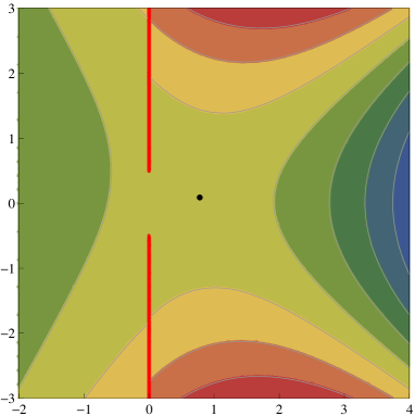
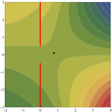
Figure 6: Contour line of the real part (left) and the imaginary part (right) of the function $\eta$, defined in (27), for $A_{0}^{+}=\{\frac{1}{2}\}$, $A^{+}=\{\frac{3}{2}\}$, $A_{0}^{-}=A^{-}=\{\}$. The red, straight lines are a possible choice for the branch cuts of $\eta$. The dot in the middle is the position of the saddle point $c\approx 0.778+0.09\,\rmi$ of $\eta$, solution of $\eta^{\prime}(c)=0$.

4.2 Relation with polylogarithms

The function $\eta$ can be expressed in terms of a polylogarithm function instead of Hurwitz zeta function, using Jonquière’s identity

$$\zeta(1-s,q)=\frac{\Gamma(s)}{(2\pi)^{s}}\Big{(}\rme^{-\frac{\rmi\pi s}{2}}\mathrm{Li}_{s}(\rme^{2\rmi\pi q})+\rme^{\frac{\rmi\pi s}{2}}\mathrm{Li}_{s}(\rme^{-2\rmi\pi q})\Big{)}\;,$$ (45)

which is valid for $s\in\mathbb{C}\backslash\{0\}$ and $0<\mathrm{Re}\,q<1$. It corresponds to the constraint $-1/2<\mathrm{Im}\,c<1/2$ for $\eta(c)$. In order to go beyond this interval, one has to make the analytic continuation across the cut $[1,\infty[$ of the polylogarithm. This can be done by adding or removing a few terms from the sum in the definition (63): for $m\in\mathbb{Z}$

$$\zeta(s,q)=\zeta(s,q+m)+\Bigg{\{}\begin{array}[]{lc}+\sum_{j=0}^{m-1}(q+j)^{-s}&\mathrm{if}\,m>0\\ -\sum_{j=1}^{-m}(q-j)^{-s}&\mathrm{if}\,m<0\end{array}\;.$$ (46)

One finds

$$\eta(c)=\mathrm{Li}_{5/2}(-\rme^{2\pi c})$$ (47)

$$\hskip 36.98857pt-\frac{8\sqrt{2}\,\rmi\pi^{2}}{3}\Bigg{(}\sum_{a\in A_{0}^{+}}(c+\rmi a)^{3/2}+\sum_{a\in A^{-}}(c+\rmi a)^{3/2}$$

$$\hskip 113.81102pt-\sum_{a\in A_{0}^{-}}(c-\rmi a)^{3/2}-\sum_{a\in A^{+}}(c-\rmi a)^{3/2}$$

$$\hskip 113.81102pt+2\,\mathrm{sgn}(\mathrm{Im}\,c)\sum_{j=1}^{|[\mathrm{Im}\,c]|}\Big{(}c-\mathrm{sgn}(\mathrm{Im}\,c)\rmi(j-\mbox{\small$\frac{1}{2}$})\Big{)}^{3/2}\Bigg{)}\;,$$

where $[x]$ is the integer closest to $x$ and $\mathrm{sgn}$ the sign function.

4.3 Expression with a regularized infinite sum

It is possible to remove completely Hurwitz zeta function from the definition (27) of $\eta(c)$ by using (46). For large $M$, the quantity $\zeta(s,q+M)$ has the asymptotics (64), and one finds for $\mathrm{Re}\,c>0$

$$\eta(c)=\lim_{M\to\infty}\frac{16\pi^{2}}{3}\,\Big{(}\frac{2}{5}\,M^{5/2}+cM^{3/2}-\frac{1+12c^{2}}{16}\,\sqrt{M}\Big{)}$$ (48)

$$-\frac{8\sqrt{2}\,\rmi\pi^{2}}{3}\,\Bigg{(}\sum_{a\in A_{0}^{+}}(c+\rmi a)^{3/2}+\sum_{a\in A^{-}}(c+\rmi a)^{3/2}+\sum_{j=0}^{M-1}\Big{(}c+\rmi(-j-\mbox{\small$\frac{1}{2}$})\Big{)}^{3/2}$$

$$\hskip 51.21495pt-\sum_{a\in A_{0}^{-}}(c-\rmi a)^{3/2}-\sum_{a\in A^{+}}(c-\rmi a)^{3/2}-\sum_{j=0}^{M-1}\Big{(}c-\rmi(-j-\mbox{\small$\frac{1}{2}$})\Big{)}^{3/2}\Bigg{)}\;.$$

This expression corresponds to adding an infinity of negative half-integers to the sets $A_{0}^{+}$ and $A^{+}$, or to the sets $A_{0}^{-}$ and $A^{-}$.

4.4 Approximate expression for large argument

For large $|c|$, one can use for $\eta$ the asymptotics (64) with $s=5/2$: $\zeta(-3/2,z)\simeq-2z^{5/2}/5+z^{3/2}/2-\sqrt{z}/8$ for $|z|\to\infty$. One has

$$\eta(c)\simeq-\frac{32\sqrt{2}\pi^{2}}{15}\,c^{5/2}-\frac{\sqrt{2}\pi^{2}}{3}\,\sqrt{c}$$ (49)

$$\hskip 36.98857pt-\frac{8\sqrt{2}\,\rmi\pi^{2}}{3}\Big{(}\sum_{a\in A_{0}^{+}}(c+\rmi a)^{3/2}+\sum_{a\in A^{-}}(c+\rmi a)^{3/2}$$

$$\hskip 156.49014pt-\sum_{a\in A_{0}^{-}}(c-\rmi a)^{3/2}-\sum_{a\in A^{+}}(c-\rmi a)^{3/2}\Big{)}\;.$$

The equation for $c$ (28) with $\eta$ replaced by its approximate value for large $|c|$ has the form

$$\frac{4\rmi}{3}\,c^{3/2}\simeq\sum_{j=1}^{m}h_{p_{j},q_{j}}(c)\;,$$ (50)

where the numbers $p_{j}$ and $q_{j}$ are positive half-integers and $h_{p,q}(c)=\sqrt{c+\rmi p}-\sqrt{c-\rmi q}$.

The function $h_{p,q}$ is a continuous bijection from the domain $\mathcal{D}=\{c\in\mathbb{C},\,\mathrm{Re}\,c>0\}$ to its image by $h_{p,q}$. Indeed, if we assume the existence of $c$ and $c^{\prime}$ such that $h_{p,q}(c)=h_{p,q}(c^{\prime})$, taking the square of $\sqrt{c+\rmi p}+\sqrt{c^{\prime}-\rmi q}=\sqrt{c^{\prime}+\rmi p}+\sqrt{c-\rmi q}$, simplifying, and taking again the square leads to $\rmi(p+q)(c-c^{\prime})=0$, hence $c=c^{\prime}$. The image by $h_{p,q}$ of $\mathcal{D}$ can thus be found by looking at the image of its boundary $\partial\mathcal{D}=\{c\in\mathbb{C},\,\mathrm{Re}\,c=0\}$. Writing $c=\rmi d$, $d\in\mathbb{R}$, one has for $p,q>0$

$$h_{p,q}(\rmi d)=\left\{\begin{array}[]{llc}\rme^{3\rmi\pi/4}(\sqrt{q-d}-\sqrt{-p-d})&&\hskip 41.25648ptd<-p\\ \rme^{\rmi\pi/4}\sqrt{d+p}+\rme^{3\rmi\pi/4}\sqrt{q-d}&&-p<d<q\\ \rme^{\rmi\pi/4}(\sqrt{d+p}-\sqrt{d-q})&&q<d\end{array}\right.\;.$$ (51)

We note that $h_{p,q}(\rmi d)\to 0$ when $d\to\pm\infty$, hence $h_{p,q}(\partial\mathcal{D})$ is a closed contour. The image by $h_{p,q}$ of $\mathcal{D}$ is the inside of this contour. All the elements $z\in h_{p,q}(\mathcal{D})$ are thus contained in the wedge $\frac{\pi}{4}<\arg z<\frac{3\pi}{4}$. But the sum of two points from this wedge still belongs to the same wedge. It implies that the right hand side of (50) is also inside the wedge if $\mathrm{Re}\,c>0$. The equality (50) then gives $\frac{\pi}{4}<\arg(\rmi c^{3/2})<\frac{3\pi}{4}$. This is only possible if $-\frac{\pi}{6}<\arg c<\frac{\pi}{6}$: all the solutions in $\mathcal{D}$ of the approximate equation (50) must verify this stronger constraint.

We conjecture that $-\frac{\pi}{6}<\arg c<\frac{\pi}{6}$ is also verified for all the solutions of the exact equation (28) for $c$. Indeed, one observes in table 1 that the constraint is verified for the first eigenstates, which are the ones where (28) differs the most from (50) since they correspond to smaller values of $|c|$.

4.5 Geometric picture of $\eta^{\prime}$

The function $\eta^{\prime}$, which appears in the equation (28) for $c$, involves sums of terms of the form $w=\pm\sqrt{c\pm\rmi a}$ with $a\in\mathbb{N}+1/2$.

Writing $w=x+\rmi y$ with $x,y\in\mathbb{R}$ and taking the real part of $w^{2}$ gives the equation $x^{2}-y^{2}=\mathrm{Re}\,c$. This is the equation of an hyperbola with foci at $\pm\sqrt{2\,\mathrm{Re}\,c}$ and perpendicular asymptotes. In the domain $\mathrm{Re}\,c>0$, the terms $w=\sqrt{c+\rmi a}$ belong to the branch of the hyperbola with $\mathrm{Re}\,w>0$, while the terms $w=-\sqrt{c-\rmi a}$ belong to the branch of the hyperbola with $\mathrm{Re}\,w<0$. The condition (12) on the sets $A_{0}^{\pm}$ and $A^{\pm}$ implies that there is the same number of points on each branch of the hyperbola, although two points can be at the same location, like in figure 7.

Furthermore, from $w=\pm\sqrt{c\pm\rmi a}$, one has also $|w+\sqrt{c}|\,|w-\sqrt{c}|=a$. This is the equation of a Cassini oval with parameter $a\in\mathbb{N}+1/2$ and foci $\pm\sqrt{c}$ located on the hyperbola.

Considering the expression (48) for $\eta^{\prime}$, one can also add to the picture of figure 7 a number $M\to\infty$ of points on each branch of the hyperbola, in the region with negative imaginary part. We did not manage, however, to find a natural geometrical interpretation for the regularization term $M^{3/2}-\frac{3}{2}\sqrt{M}c\simeq(M-c)^{3/2}$.

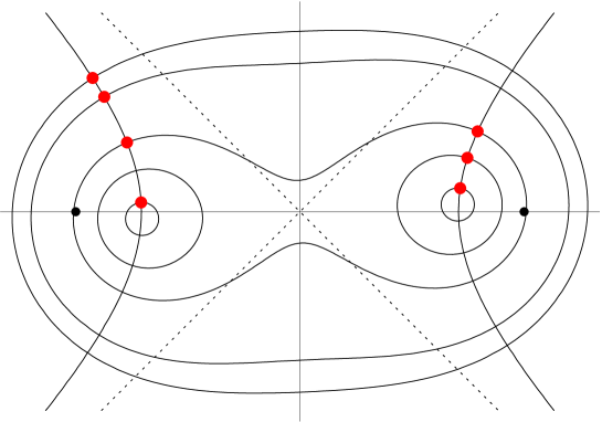
Figure 7: Geometric representation in the complex plane of the terms of the $4$ summations in expression (27) for $\eta^{\prime}(c)=0$. The eigenstate chosen is indexed by the sets $A_{0}^{+}=\{\frac{1}{2},\frac{3}{2},\frac{5}{2}\}$, $A^{-}=\{\frac{1}{2}\}$, $A_{0}^{-}=\{\frac{9}{2}\}$, $A^{+}=\{\frac{1}{2},\frac{5}{2},\frac{11}{2}\}$, and one has $c\approx 2.397+0.218\,\rmi$. The red points, located at intersections between a hyperbola and Cassini ovals, represent the complex numbers $-\sqrt{c-\rmi a}$, $a\in A_{0}^{-}\cup A^{+}$ and $\sqrt{c+\rmi a}$, $a\in A_{0}^{+}\cup A^{-}$. The two smaller, black dots located on the horizontal axis at $\pm\sqrt{2\,\mathrm{Re}\,c}$ are the foci of the hyperbola, and the two perpendicular dotted lines its asymptotes.

5 Numerical evaluations

The parameter $c$ solution of (28) and the quantity $\eta(c)$ defined in (27) and related to the eigenvalues of the Markov matrix by (34), are evaluated numerically for the first eigenstates in this section.

5.1 First excited state

The two excited states whose eigenvalues have the smallest real part (gap) correspond to either $A_{0}^{+}=A^{+}=\{\frac{1}{2}\}$, $A_{0}^{-}=A^{-}=\{\}$ or $A_{0}^{+}=A^{+}=\{\}$, $A_{0}^{-}=A^{-}=\{\frac{1}{2}\}$. In both cases, the solution of (28) is $c=0.559534\ldots\in\mathbb{R}$. From (27), this value of $c$ is solution of $\mathrm{Li}_{3/2}(-\rme^{2\rmi\pi c})=2\rmi\pi(\sqrt{2c+\rmi}-\sqrt{2c-\rmi})$, which is the same as equation (27) of [16] with $u=c/2$. Then, the corresponding eigenvalue of the Markov matrix is (34) with $P=\pm 1$ and $\eta(c)=\mathrm{Li}_{5/2}(-\rme^{2\pi c})-\frac{4\rmi\pi^{2}}{3}((2c+\rmi)^{3/2}-(2c-\rmi)^{3/2})=13.0184\ldots$. This matches with equation (30) of [16].

5.2 Higher excited states

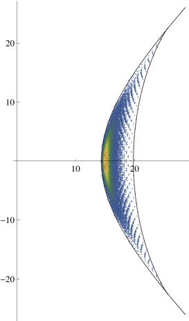
Figure 10: Values in the complex plane of $\eta(c)/(\sqrt{2\pi}Q^{5/4})$ for all $589128$ eigenstates corresponding to an index $Q=30$, with $\eta$ defined in (27) and $Q$ defined in (15). The corresponding eigenvalues are given in terms of $\eta(c)$ in (34). Each small square is coloured according to the number of eigenstates within the square, with smaller numbers at the border of the crescent. The curve at the inner edge of the crescent (right) is given by the exact value of $\eta(c)$ with the sets given before (52) with $\alpha\in[0,1]$. The curve at the outer edge of the crescent (left) is given by the asymptotics (56) with $1/10<\alpha<10$.

The equation (28) for $c$ can be solved numerically for eigenstates beyond the gap. In figure 8, $\eta(c)$ and $c$ are plotted for all the eigenstates whose index $Q$, defined in (15), is between $1$ and $7$. The numerical values of $\eta(c)$ and $c$ are also given in table 1 for all the eigenstates with $Q$ between $0$ and $5$. The values of $\eta(c)$ for all the eigenstates with given $Q$ accumulate for large $Q$ in a crescent shape, see figure 10.

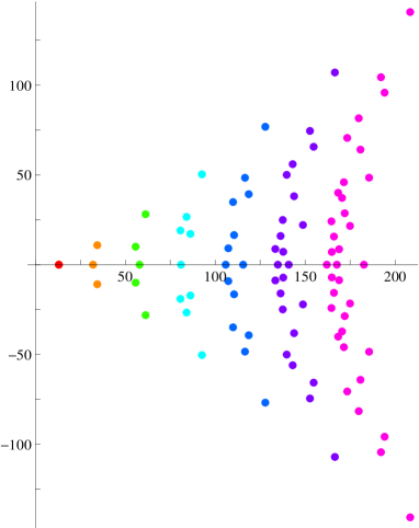
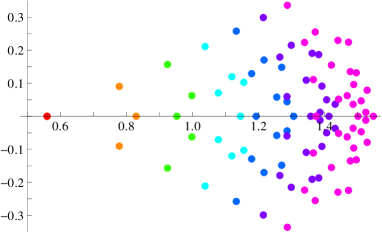
Figure 8: On the left, values of $\eta(c)/\sqrt{2\pi}$ for the first eigenstates, with $\eta$ defined in (27). The corresponding eigenvalues are given in terms of $\eta(c)$ in (34). On the right, intermediate parameter $c$ solution of $\eta^{\prime}(c)=0$ and used in the calculation of the eigenvalues. The dots are coloured according to the value of the index $Q$, defined in (15), which increases from left to right on both graphs. All the eigenstates with $Q$ between $1$ and $7$ are represented.

Q	$(A_{0}^{+},A^{-})$	$(A_{0}^{-},A^{+})$	Degeneracy	$c$	$\displaystyle\frac{\eta(c)}{\sqrt{2\pi}}$
0	$()$	$()$	1	Indeterminate	Indeterminate
1	$(\frac{1}{2})$	$(\frac{1}{2})$	2	$0.559534$	$13.0184$
2	$(\frac{1}{2},\frac{1}{2})$	$(\frac{1}{2},\frac{1}{2})$	1	$0.82937$	$32.0353$
2	$(\frac{1}{2})$	$(\frac{3}{2})$	2	$0.778306+0.0902648\,\rmi$	$34.3768-10.8732\,\rmi$
2	$(\frac{3}{2})$	$(\frac{1}{2})$	2	$0.778306-0.0902648\,\rmi$	$34.3768+10.8732\,\rmi$
3	$(\frac{1}{2},\frac{1}{2})$	$(\frac{1}{2},\frac{3}{2})$	2	$0.998165+0.0624517\,\rmi$	$55.6906-10.0233\,\rmi$
3	$(\frac{1}{2},\frac{3}{2})$	$(\frac{1}{2},\frac{1}{2})$	2	$0.998165-0.0624517\,\rmi$	$55.6906+10.0233\,\rmi$
3	$(\frac{3}{2})$	$(\frac{3}{2})$	2	$0.952726$	$57.8869$
3	$(\frac{1}{2})$	$(\frac{5}{2})$	2	$0.924474+0.156784\,\rmi$	$61.2404-28.1045\,\rmi$
3	$(\frac{5}{2})$	$(\frac{1}{2})$	2	$0.924474-0.156784\,\rmi$	$61.2404+28.1045\,\rmi$
4	$(\frac{1}{2},\frac{1}{2})$	$(\frac{3}{2},\frac{3}{2})$	1	$1.15545+0.102772\,\rmi$	$80.6252-19.0466\,\rmi$
4	$(\frac{3}{2},\frac{3}{2})$	$(\frac{1}{2},\frac{1}{2})$	1	$1.15545-0.102772\,\rmi$	$80.6252+19.0466\,\rmi$
4	$(\frac{1}{2},\frac{3}{2})$	$(\frac{1}{2},\frac{3}{2})$	6	$1.14571$	$80.9397$
4	$(\frac{1}{2},\frac{1}{2})$	$(\frac{1}{2},\frac{5}{2})$	2	$1.11938+0.119929\,\rmi$	$84.0436-26.6439\,\rmi$
4	$(\frac{1}{2},\frac{5}{2})$	$(\frac{1}{2},\frac{1}{2})$	2	$1.11938-0.119929\,\rmi$	$84.0436+26.6439\,\rmi$
4	$(\frac{3}{2})$	$(\frac{5}{2})$	2	$1.07836+0.0707095\,\rmi$	$86.1719-17.1468\,\rmi$
4	$(\frac{5}{2})$	$(\frac{3}{2})$	2	$1.07836-0.0707095\,\rmi$	$86.1719+17.1468\,\rmi$
4	$(\frac{1}{2})$	$(\frac{7}{2})$	2	$1.03814+0.211083\,\rmi$	$92.5825-50.3354\,\rmi$
4	$(\frac{7}{2})$	$(\frac{1}{2})$	2	$1.03814-0.211083\,\rmi$	$92.5825+50.3354\,\rmi$
5	$(\frac{1}{2},\frac{1}{2},\frac{3}{2})$	$(\frac{1}{2},\frac{1}{2},\frac{3}{2})$	2	$1.30655$	$105.785$
5	$(\frac{1}{2},\frac{3}{2})$	$(\frac{3}{2},\frac{3}{2})$	2	$1.28648+0.0440786\,\rmi$	$107.25-9.1338\,\rmi$
5	$(\frac{3}{2},\frac{3}{2})$	$(\frac{1}{2},\frac{3}{2})$	2	$1.28648\,-0.0440786\,\rmi$	$107.25+9.1338\,\rmi$
5	$(\frac{1}{2},\frac{1}{2})$	$(\frac{3}{2},\frac{5}{2})$	2	$1.27024\,+0.14822\,\rmi$	$109.865-34.8779\,\rmi$
5	$(\frac{3}{2},\frac{5}{2})$	$(\frac{1}{2},\frac{1}{2})$	2	$1.27024\,-0.14822\,\rmi$	$109.865+34.8779\,\rmi$
5	$(\frac{1}{2},\frac{3}{2})$	$(\frac{1}{2},\frac{5}{2})$	6	$1.25528\,+0.0580091\,\rmi$	$110.44-16.5029\,\rmi$
5	$(\frac{1}{2},\frac{5}{2})$	$(\frac{1}{2},\frac{3}{2})$	6	$1.25528\,-0.0580091\,\rmi$	$110.44+16.5029\,\rmi$
5	$(\frac{5}{2})$	$(\frac{5}{2})$	2	$1.19288$	$115.49$
5	$(\frac{1}{2},\frac{1}{2})$	$(\frac{1}{2},\frac{7}{2})$	2	$1.21666\,+0.170272\,\rmi$	$116.513-48.4036\,\rmi$
5	$(\frac{1}{2},\frac{7}{2})$	$(\frac{1}{2},\frac{1}{2})$	2	$1.21666\,-0.170272\,\rmi$	$116.513+48.4036\,\rmi$
5	$(\frac{3}{2})$	$(\frac{7}{2})$	2	$1.17919\,+0.129087\,\rmi$	$118.594-39.2823\,\rmi$
5	$(\frac{7}{2})$	$(\frac{3}{2})$	2	$1.17919\,-0.129087\,\rmi$	$118.594+39.2823\,\rmi$
5	$(\frac{1}{2})$	$(\frac{9}{2})$	2	$1.13278\,+0.257656\,\rmi$	$127.805-76.8167\,\rmi$
5	$(\frac{9}{2})$	$(\frac{1}{2})$	2	$1.13278\,-0.257656\,\rmi$	$127.805+76.8167\,\rmi$

Table 1: Values of $c$ and $\eta(c)/\sqrt{2\pi}$ for the first eigenstates, with $\eta$ defined in (27). The corresponding eigenvalues are given in terms of $\eta(c)$ in (34). The intermediate parameter $c$ solution of $\eta^{\prime}(c)=0$ is used in the calculation of the eigenvalues. The index $Q$ in the first column is defined in (15). All the eigenstates with $Q$ between $0$ and $5$ are given in the table. The columns $2$ and $3$ give sorted lists of the elements of $A_{0}^{\pm}$ and $A^{\mp}$ put together. An element contained in both $A_{0}^{\pm}$ and $A^{\mp}$ is given twice in the list. Column $4$ gives the number of eigenstates with the same value of $\eta(c)$.

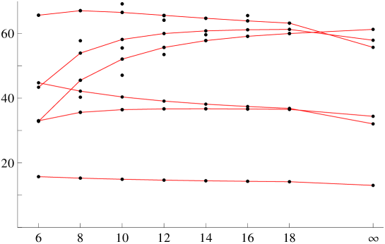
Figure 9: Bottom of the spectrum of TASEP for small system size $L$ with $N=L/2$ particles (density $\rho=1/2$). The black dots correspond to $-2L^{3/2}\,\mathrm{Re}\,E$ for each eigenvalue $E$. The points for finite $L$ are obtained from exact diagonalization of the Markov matrix $M$. The rightmost points represent the $L\to\infty$ limit given by (34). The eigenvalues linked correspond to a similar choice of integers $k_{j}$ in the solution (7) of the Bethe ansatz equations.

We observe in table 1 that the eigenstates forming the inner part (where $\mathrm{Re}\,\eta(c)$ is larger) of the crescent correspond to either $A_{0}^{+}=\{a\}$, $A^{+}=\{Q-a\}$, $A_{0}^{-}=A^{-}=\{\}$ or to $A_{0}^{-}=\{Q-a\}$, $A^{-}=\{a\}$, $A_{0}^{+}=A^{+}=\{\}$, with $a$ half integer between $\frac{1}{2}$ and $Q-\frac{1}{2}$. At large $Q$ with $\alpha=a/Q$ fixed, (28) and (49) imply

$$c\simeq\frac{3^{2/3}}{2^{4/3}}\,(\rme^{-\rmi\pi/4}\sqrt{\alpha}+\rme^{\rmi\pi/4}\sqrt{1-\alpha})^{2/3}Q^{1/3}$$ (52)

$$\eta(c)\simeq\frac{8\sqrt{2}\pi^{2}}{3}\,(\rme^{\rmi\pi/4}\alpha^{3/2}+\rme^{-\rmi\pi/4}(1-\alpha)^{3/2})Q^{3/2}\;.$$ (53)

The first equation indicates that the parameter $c$ belongs to the arc of circle $|c|\simeq(3/4)^{2/3}Q^{1/3}$, $-\frac{\pi}{6}<\arg c<\frac{\pi}{6}$. The second equation shows that $-\frac{\pi}{4}<\arg\eta(c)<\frac{\pi}{4}$ for large $Q$.

All eigenstates in the bulk of the crescent (except for a negligible fraction of them when $Q\to\infty$) correspond to sets $A_{0}^{\pm}$, $A^{\pm}$ with typical elements scaling as $\sqrt{Q}$ and of cardinal $m_{\pm}\simeq\mu_{\pm}\sqrt{Q}$. We define for $Q^{-1/2}\ll\rmd u\ll 1$ smooth functions $\theta$ and $\overline{\theta}$ such that $2\theta(u)\sqrt{Q}\,\rmd u$ (respectively $2\overline{\theta}(u)\sqrt{Q}\,\rmd u$) is the number of elements of $A_{0}^{+}$ (resp. $A_{0}^{-}$) plus the number of elements of $A^{-}$ (resp. $A^{+}$) in the interval $\sqrt{Q}[u,u+du]$. They verify the normalizations $\int_{0}^{\infty}\rmd u\,\theta(u)=\int_{0}^{\infty}\rmd u\,\overline{\theta}(u)=\mu_{+}+\mu_{-}$ and $\int_{0}^{\infty}\rmd u\,u\,\theta(u)=\int_{0}^{\infty}\rmd u\,u\,\overline{\theta}(u)=1$. Writing $c=\chi\sqrt{Q}$, (49) gives for large $Q$

$$\hskip 14.22636pt\frac{\eta(c)}{Q^{5/4}}\simeq-\frac{32\sqrt{2}\pi^{2}}{15}\,\chi^{5/2}-\frac{8\sqrt{2}\,\rmi\pi^{2}}{3}\,\int_{0}^{\infty}\rmd u\,\Big{(}\theta(u)(\chi+\rmi u)^{3/2}-\overline{\theta}(u)(\chi-\rmi u)^{3/2}\Big{)}\;.$$ (54)

The total number of ways to choose the elements of the sets $A_{0}^{+}$ and $A^{-}$ in the interval $[u,u+\rmd u]$ is equal to

$$\omega(u)\simeq\int_{0}^{2\theta(u)}\rmd\sigma\,{\sqrt{Q}\,\rmd u\choose\sigma\sqrt{Q}\,\rmd u}{\sqrt{Q}\,\rmd u\choose(2\theta(u)-\sigma)\sqrt{Q}\,\rmd u}\simeq\rme^{2\sqrt{Q}\,s(\theta(u))\,\rmd u}\;,$$ (55)

with $s(\varphi)=-\varphi\log\varphi-(1-\varphi)\log(1-\varphi)$. Similarly for $A_{0}^{-}$ and $A^{+}$, the number of choices is $\overline{\omega}(u)\simeq\exp[2\sqrt{Q}\,s(\overline{\theta}(u))\,\rmd u]$. The total number of eigenstates corresponding to $\theta$ and $\overline{\theta}$ is then equal to $\Omega[\theta,\overline{\theta}]\simeq\exp[2\sqrt{Q}\int_{0}^{\infty}\rmd u\,(s(\theta(u))+s(\overline{\theta}(u)))]$.

The outer part (where $\mathrm{Re}\,\eta(c)$ is smaller) of the crescent in figure 8 is reached from the bulk of the crescent for functions $\theta$ and $\overline{\theta}$ such that $\log\Omega[\theta,\overline{\theta}]$ vanishes. It corresponds to $\theta(u)$ and $\overline{\theta}(u)$ equal to either $0$ or $1$, i.e. the sets $A_{0}^{+}=A^{-}$ and $A_{0}^{-}=A^{+}$ are both composed by a finite reunion of intervals of the form $\{a,a+1,\ldots,b\}$ with $b-a$ scaling as $\sqrt{Q}$. For simplicity, we consider only the case of sets equal to only one interval: we write $A_{0}^{+}=A^{-}=[\sqrt{Q}\,x,\sqrt{Q}\,y]$ and $A_{0}^{-}=A^{+}=[\sqrt{Q}\,\overline{x},\sqrt{Q}\,\overline{y}]$ and call $\mu=\mu_{+}=\mu_{-}$. The normalization conditions for $\theta$ and $\overline{\theta}$ imply $y-x=\overline{y}-\overline{x}=\mu$ and $(y^{2}-x^{2})+(\overline{y}^{2}-\overline{x}^{2})=1$. Writing $\frac{x+y}{2}=\frac{1}{4\mu}+\lambda$ and $\frac{\overline{x}+\overline{y}}{2}=\frac{1}{4\mu}-\lambda$, the positivity of $x$ and $\overline{x}$ implies $\frac{\mu}{2}-\frac{1}{4\mu}\leq\lambda\leq\frac{1}{4\mu}-\frac{\mu}{2}$, thus $0\leq\mu\leq 1/\sqrt{2}$. The quantity $Q^{-5/4}\eta(\chi\sqrt{Q})$ depends only on $\chi$ and on the parameters $\lambda$ and $\mu$. We observe numerically that the values of $\eta$ with smallest real part correspond to the two extremal choices for $\lambda$: $\lambda=\frac{\mu}{2}-\frac{1}{4\mu}$ and $\lambda=\frac{1}{4\mu}-\frac{\mu}{2}$. Since the two values of $\lambda$ are exchanged by $\mu\to(2\mu)^{-1}$, it is sufficient to consider only one of them and take $\mu\in\mathbb{R}^{+}$. A parametric expression with parameter $\alpha=\sqrt{2}\mu$ for the outer part of the crescent is then given by

$$\hskip 28.45274pt\frac{\eta(c)}{Q^{5/4}}=-\frac{32\sqrt{2}\pi^{2}}{15}\Big{[}\Big{(}\chi+\frac{\rmi\alpha}{\sqrt{2}}\Big{)}^{5/2}+\Big{(}\chi-\frac{\rmi\alpha^{-1}}{\sqrt{2}}\Big{)}^{5/2}-\Big{(}\chi+\frac{\rmi(\alpha-\alpha^{-1})}{\sqrt{2}}\Big{)}^{5/2}\Big{]}\;$$ (56)

with $c=\chi\sqrt{Q}$ solution of (28). When $\alpha\to 0$, the solution is $c\simeq 2^{-7/6}3^{2/3}\rme^{\rmi\pi/6}\alpha^{1/3}\sqrt{Q}$ and $\eta(c)\simeq 2^{13/4}3^{-1}\pi^{2}\rme^{-\rmi\pi/4}\alpha^{-1/2}Q^{5/4}$. The solution for $\alpha\to\infty$ follows from $\alpha\to\alpha^{-1}$ and complex conjugation. We find again that the edges of the crescent verify $\arg c\to\pm\pi/6$ and $\arg\eta(c)\to\mp\pi/4$. The point of the crescent with smallest real part corresponds to $\alpha=1$, for which $\eta(c)/\sqrt{2\pi}=32\pi^{3/2}z^{1/4}/15\approx 14.376662$ with $z$ the largest real root of $395307-642600z+212544z^{2}+512z^{3}=0$.

	$(\frac{1}{2})(\frac{1}{2})$	$(\frac{1}{2},\frac{1}{2})(\frac{1}{2},\frac{1}{2})$	$(\frac{1}{2})(\frac{3}{2})$	$(\frac{1}{2},\frac{1}{2})(\frac{1}{2},\frac{3}{2})$	$(\frac{3}{2})(\frac{3}{2})$
$L=6$	$15.7089$	$44.7384$	$32.9964-21.8944\,\rmi$	$65.6302-23.2962\,\rmi$	$43.3573$
$L=8$	$15.2587$	$42.1495$	$35.6021-20.2845\,\rmi$	$67.0315-21.2037\,\rmi$	$53.9139$
$L=10$	$14.9056$	$40.3553$	$36.4302-18.8088\,\rmi$	$66.4897-19.3528\,\rmi$	$58.1394$
$L=12$	$14.6395$	$39.0764$	$36.6691-17.6584\,\rmi$	$65.5817-17.9374\,\rmi$	$59.9675$
$L=14$	$14.4357$	$38.1283$	$36.6883-16.7714\,\rmi$	$64.682-16.8607\,\rmi$	$60.7825$
$L=16$	$14.2759$	$37.4006$	$36.6216-16.077\,\rmi$	$63.878-16.0264\,\rmi$	$61.1294$
$L=18$	$14.1477$	$36.8258$	$36.5227-15.5226\,\rmi$	$63.1801-15.3657\,\rmi$	$61.2461$
BST	$13.0184$	$32.0353$	$34.3771-10.8731\,\rmi$	$55.6919-10.0232\,\rmi$	$57.8772$
Exact result	$13.0184$	$32.0353$	$34.3768-10.8732\,\rmi$	$55.6906-10.0233\,\rmi$	$57.8869$

Table 2: Some eigenvalues of TASEP for small system size $L$ with $N=L/2$ particles (density $\rho=1/2$). Each column corresponds to a given choice of the sets $A_{0}^{\pm}$ and $A^{\mp}$ which index the first eigenstates in the Bethe ansatz formulation. At the top of each column are sorted lists of the elements of $A_{0}^{\pm}$ and $A^{\mp}$ put together. An element contained in both $A_{0}^{\pm}$ and $A^{\mp}$ is given twice in the list. The numbers correspond to $-2L^{3/2}\,\mathrm{Re}\,E$ for an eigenvalue $E$. The penultimate row gives the extrapolation of these numbers using BST algorithm with exponent $\omega=1$. The last line is the exact limit $L\to\infty$ given by (34).

5.3 Numerical checks by exact diagonalization

We checked by exact diagonalization for small $L$ the numerical values of table 1 obtained from the large $L$ limit (34). We used BST algorithm (see e.g. [78]) to extrapolate the data from $6\leq L\leq 18$, $\rho=1/2$ up to $L\to\infty$. BST algorithm consists in fitting the numerical data with a Taylor series in $L^{-\omega}$. We have chosen $\omega=1$ in our computations.

The results, given in table 2, are in good agreement with the numerical values of table 1. A difficulty in doing the extrapolation is that one must choose for all $L$ the ”same” eigenvalue, with numbers $k_{j}$ in (8) and (9) corresponding to the same sets $A_{0}^{\pm}$, $A^{\pm}$. Indeed, we observe in figure 9 that there are many crossings of eigenvalues as $L$ increases from small values to infinity. It means that Bethe ansatz is somewhat needed in order to perform the extrapolation on the numerical data from exact diagonalization.

6 Conclusion

Using Bethe ansatz, we studied the lower edge of the spectrum of the Markov matrix and of the transfer matrix of TASEP on a ring. In the lower part of the spectrum, eigenvalues have real part scaling as $L^{-3/2}$ when the system size $L$ goes to infinity with fixed density of particles. It corresponds to a relaxation time growing as $L^{z}$ with the dynamical exponent $z=3/2$ of the KPZ universality class.

We found that each eigenstate is characterized by a function $\eta$, defined in (27): the corresponding eigenvalue of the Markov matrix is written (34) in terms of $\eta(c)$, where the complex number $c$ is determined by the saddle point equation $\eta^{\prime}(c)=0$. This property extends to the eigenvalues of the transfer matrix (43), (44).

It would be interesting to generalize the present work to ASEP, where particles can hop in both directions with different rates $p$ and $q$. Especially interesting would be the crossover to KPZ scale $p-q\sim 1/\sqrt{L}$ and the crossover to equilibrium scale $p-q\sim 1/L$. The Bethe ansatz for general ASEP is however much more complicated than the one for TASEP, since the unknown parameter $b$ is replaced by a function, solution of a nonlinear integral equation which replaces the equation (9) for the constant $b$. Currently, only the first terms in the expansion for large $(p-q)\sqrt{L}$ of the gap are known exactly for ASEP [17], see also [79] for results by exact diagonalization of small systems.

Another possible direction of study would be to consider the eigenstates corresponding to the lowest eigenvalues for TASEP, which would be necessary in order to compute the crossover between transient and stationary fluctuations of the current. This is usually a difficult problem. It should be noted, however, that once the eigenvalues are known, the determination of the eigenvectors reduces to a linear problem. Moreover, since the first eigenvalues of the whole transfer matrix depend only on the quantity $\eta(c)$, it is tempting to believe that components of the eigenvectors can be expressed in terms of $\eta(c)$ in the thermodynamic limit.

Appendix A Some properties of the function $\psi$

Let $g$ be the function from $\mathbb{C}\backslash\mathbb{R}^{-}$ to $\mathbb{C}\backslash(\rme^{\rmi\pi\rho-b_{0}}[1,\infty[\,\cup\,\rme^{-\rmi\pi\rho-b_{0}}[1,\infty[)$ defined by

$$g(y)=\frac{1-y}{y^{\rho}}\;,$$ (57)

with $0<\rho<1$ and $b_{0}$ defined in (19). It was argued in Appendix A of [60] that $g$ is a bijection. With the usual definition of the logarithm in $y^{\rho}=\rme^{\rho\log(y)}$, the interval $\mathbb{R}^{-}$ is a branch cut of $g$. The reciprocal function $g^{-1}$ also has a branch cut, equal to $(\,\rme^{\rmi\pi\rho-b_{0}}[1,\infty[\,)\,\cup\,(\,\rme^{-\rmi\pi\rho-b_{0}}[1,\infty[\,)$, which is the image by $g$ of its branch cut (i.e. the limit $\epsilon\to 0$, $\epsilon>0$ of the set $\{g(-y+\rmi\epsilon),y\in\mathbb{R}^{-}\}\cup\{g(-y-\rmi\epsilon),y\in\mathbb{R}^{-}\}$).

The function $\psi$, defined as the logarithm of $g^{-1}$, is the solution of the implicit equation (6) with the additional condition $-\pi<\mathrm{Im}\,\psi(z)<\pi$. It verifies in particular $\psi(0)=0$. The function $\psi$ has the same branch cuts as $g^{-1}$, since the image by $g^{-1}$ of the cut of $g^{-1}$ is the cut of $g$, $\mathbb{R}^{-}$, which is also the cut of the logarithm. The value of $\psi$ at the branch points $\rme^{\pm\rmi\pi\rho-b_{0}}$ is

$$\psi(\rme^{\pm\rmi\pi\rho-b_{0}-\epsilon})\underset{\epsilon\to 0}{\to}\log\Big{(}\frac{\rho}{1-\rho}\Big{)}\mp\rmi\pi\quad\mathrm{with}\;-\pi<\arg\epsilon<\pi\;.$$ (58)

The expansion of $\psi$ near the branch points can be obtained by inserting $z=\rme^{\pm\rmi\pi\rho-b_{0}-\epsilon}$ and the expansion $\psi(z)=\log(\rho/(1-\rho))\mp\rmi\pi+\sum_{k=0}^{\infty}f_{k}\epsilon^{k/2}$ in (6) and solving for the $f_{k}$. For small $\epsilon$ with $-\pi<\arg\epsilon<\pi$, one finds

$$\psi(\rme^{\pm\rmi\pi\rho-b_{0}-\epsilon})=\log\Big{(}\frac{\rho}{1-\rho}\Big{)}\mp\rmi\pi\pm\frac{\rmi\sqrt{2}\sqrt{\epsilon}}{\sqrt{\rho(1-\rho)}}+\frac{(1-2\rho)\epsilon}{3\rho(1-\rho)}$$

$$\hskip 85.35826pt\mp\frac{\rmi(1-\rho+\rho^{2})\epsilon^{3/2}}{9\sqrt{2}(\rho(1-\rho))^{3/2}}-\frac{(1+\rho)(2-\rho)(1-2\rho)\epsilon^{2}}{135\rho^{2}(1-\rho)^{2}}$$

$$\hskip 85.35826pt\pm\frac{\rmi(1-\rho+\rho^{2})^{2}\epsilon^{5/2}}{540\sqrt{2}(\rho(1-\rho))^{5/2}}+\mathcal{O}\left(\epsilon^{3}\right)\;.$$ (59)

An interesting property of the function $\psi$ is that the derivative $\psi^{\prime}(z)$ can be expressed as a function of $\psi(z)$ only. Indeed writing $z$ as a function of $\psi(z)$ using (6) and taking the derivative with respect to $z$, one finds

$$\psi^{\prime}(z)=-\frac{\rme^{\rho\psi(z)}}{\rho+(1-\rho)\rme^{\psi(z)}}\;.$$ (60)

This property is used in section 2 to compute integrals where the integrand depends on $\psi(z)$, as it allows to explicitly perform the change of variable $y=\psi(z)$.

Appendix B Euler Maclaurin formula with square root singularity

In this appendix, we derive the asymptotic expansion of

$$S_{L,M}(d)=\sum_{j=1}^{M}f\Big{(}\frac{j+d}{L}\Big{)}\;$$ (61)

for large $L$, with $d$ and $\mu=M/L$ taken fixed, in the case where $f(x)\sim\sqrt{x}$ for $x\to 0$. More specifically, we consider $f(x)$ of the form

$$f(x)=\sum_{k=0}^{\infty}f_{k}\,x^{k/2}\;.$$ (62)

We require this expansion to be valid for all $x$ such that either $0\leq\arg x\leq\arg(d+1)$ or $\arg(d+1)\leq\arg x\leq 0$ depending on whether $d$ is in the upper half or in the lower half of the complex plane.

We introduce the Hurwitz zeta function (see e.g. [80], Section 25.11)

$$\zeta(s,q)=\sum_{j=0}^{\infty}(j+q)^{-s}\;.$$ (63)

This definition converges when $\mathrm{Re}\,s>1$, $q\not\in-\mathbb{N}$. For fixed $q$, $\zeta(s,q)$ can be continued to a holomorphic function of $s$ in $\mathbb{C}\backslash\{1\}$, with a simple pole at $s=1$. Then, for all $s\neq 1$, $\zeta(s,q)$ can be analytically continued to a holomorphic function of the variable $q$ in the domain $\mathbb{C}\backslash\mathbb{R}^{-}$. Hurwitz zeta function verifies the asymptotic expansion for large $|q|$, $-\pi<\arg\,q<\pi$, $s\neq 0$

$$\zeta(1-s,q)\underset{|q|\to\infty}{\simeq}-\frac{q^{s}}{s}\sum_{r=0}^{\infty}{s\choose r}\frac{B_{r}}{q^{r}}\;,$$ (64)

where the $B_{r}$ are Bernoulli numbers: $B_{0}=1$, $B_{1}=-1/2$, $B_{2}=1/6$, $B_{3}=0$, $B_{4}=-1/30$, … , $B_{r}=0$ for $r$ odd $\geq 3$.

The large $L$ asymptotics of the sum (61) can be obtained by writing it in terms of Hurwitz zeta function as

$$S_{L,\mu L}(d)=\sum_{k=0}^{\infty}\frac{f_{k}}{L^{k/2}}\Big{[}\zeta(-\mbox{\small$\frac{k}{2}$},\,d+1)-\zeta(-\mbox{\small$\frac{k}{2}$},\,\mu L+d+1)\Big{]}\;.$$ (65)

Indeed, by analytic continuation in $s$, one can always use (63) to write $\zeta(s,q)-\zeta(s,q+M)$ as a finite sum even when $\mathrm{Re}\,s$ is not larger than $1$. Applying (64) for the second $\zeta$, one finds for $\mu>0$ the asymptotic expansion

$$\sum_{j=1}^{\mu L}f\Big{(}\frac{j+d}{L}\Big{)}\simeq L\Big{(}\int_{0}^{\mu+\frac{d+1}{L}}\rmd u\,f(u)\Big{)}+\sum_{r=1}^{\infty}\frac{B_{r}}{r!L^{r-1}}f^{(r-1)}\Big{(}\mu+\frac{d+1}{L}\Big{)}$$

$$\hskip 193.47873pt+\sum_{k=0}^{\infty}\frac{f_{k}}{L^{k/2}}\,\zeta(-\mbox{\small$\frac{k}{2}$},\,d+1)\;,$$ (66)

with coefficients $f_{k}$ given by (62). The sum over $r$ in the previous expression is the usual Euler-Maclaurin formula corresponding to the upper bound $j=\mu L$ of the sum (61). The sum over $k$ corresponds to the lower bound $j=1$ of the sum (61): there, one can not use the usual Euler-Maclaurin formula since the derivatives $f^{(r-1)}(0)$ are infinite. One can in fact write the sum over $r$ in the previous equation in a similar form as the sum over $k$:

$$\int_{\mu}^{\mu+\frac{a}{L}}\rmd u\,f(u)+\sum_{r=1}^{\infty}\frac{B_{r}\,f^{(r-1)}(\mu+\frac{a}{L})}{r!\,L^{r}}=-\sum_{r=1}^{\infty}\frac{f^{(r-1)}(\mu)\,\zeta(1-r,a)}{(r-1)!\,L^{r}}\;,$$ (67)

which is a consequence of the identity for $r\in\mathbb{N}^{*}$

$$B_{r}(z)=\sum_{k=0}^{r}{r\choose k}B_{r-k}\,z^{k}=-r\zeta(1-r,z)\;,$$ (68)

where $B_{r}(z)$ is the $r$-th Bernoulli polynomial.

We also treat the case of a function $f$ with square root singularities at both ends $j=1$ and $j=N=\rho L$ of the sum (61):

$$f(x)=\sum_{k=0}^{\infty}f_{k}\,x^{k/2}=\sum_{k=0}^{\infty}\bar{f}_{k}\,(\rho-x)^{k/2}\;.$$ (69)

This is the case used in section 3. We assume that the first expansion is valid for $0\leq\arg x\leq\arg(d+1)$ and the second for $\arg(-d)\leq\arg(\rho-x)\leq 0$ (if $d$ is in the upper half of $\mathbb{C}$; otherwise, one can replace $f(x)$ by $f(\rho-x)$ and $d$ by $-d-1$). Then, one can introduce an intermediate point $M=\mu L$, $0<\mu<\rho$ and write

$$\sum_{j=1}^{N}f\Big{(}\frac{j+d}{L}\Big{)}=\sum_{j=1}^{M}f\Big{(}\frac{j+d}{L}\Big{)}+\sum_{j=1}^{N-M}f\Big{(}\rho-\frac{j-d-1}{L}\Big{)}\;.$$ (70)

Using the relation

$$B_{r}(1-z)=(-1)^{r}B_{r}(z)\;$$ (71)

on the Bernoulli polynomials, we observe that all the Bernoulli numbers from (B) cancel. One finds for $\rho>0$ the asymptotic expansion

$$\begin{picture}(0.0,0.0)(2.0,-8.5)\put(0.0,0.0){\line(1,0){107.0}} \put(0.0,-29.0){\line(1,0){107.0}} \put(0.0,0.0){\line(0,-1){29.0}} \put(107.0,0.0){\line(0,-1){29.0}} \end{picture}\sum_{j=1}^{\rho L}f\Big{(}\frac{j+d}{L}\Big{)}\simeq L\Big{(}\int_{0}^{\rho}\rmd u\,f(u)\Big{)}+\sum_{k=0}^{\infty}\frac{f_{k}}{L^{k/2}}\,\zeta(-\mbox{\small$\frac{k}{2}$},\,d+1)$$ (72)

$$\hskip 170.71652pt+\sum_{k=0}^{\infty}\frac{\bar{f}_{k}}{L^{k/2}}\,\zeta(-\mbox{\small$\frac{k}{2}$},\,-d)\;,$$

with coefficients $f_{k}$ and $\bar{f}_{k}$ given by (69) and $\zeta$ the Hurwitz zeta function (63).

References

References

- [1] B. Derrida. An exactly soluble non-equilibrium system: the asymmetric simple exclusion process. Phys. Rep., 301:65–83, 1998.
- [2] G.M. Schütz. Exactly solvable models for many-body systems far from equilibrium. Volume 19 of Phase Transitions and Critical Phenomena. San Diego: Academic, 2001.
- [3] O. Golinelli and K. Mallick. The asymmetric simple exclusion process: an integrable model for non-equilibrium statistical mechanics. J. Phys. A: Math. Gen., 39:12679–12705, 2006.
- [4] T. Sasamoto. Fluctuations of the one-dimensional asymmetric exclusion process using random matrix techniques. J. Stat. Mech., 2007:P07007.
- [5] K. Mallick. Some exact results for the exclusion process. J. Stat. Mech., 2011:P01024.
- [6] M. Hairer. Singular stochastic PDEs. Proceedings of the ICM, 2014.
- [7] M. Kardar, G. Parisi, and Y.-C. Zhang. Dynamic scaling of growing interfaces. Phys. Rev. Lett., 56:889–892, 1986.
- [8] T. Halpin-Healy and Y.-C. Zhang. Kinetic roughening phenomena, stochastic growth, directed polymers and all that. Aspects of multidisciplinary statistical mechanics. Phys. Rep., 254:215–414, 1995.
- [9] T. Sasamoto and H. Spohn. The 1+1-dimensional Kardar-Parisi-Zhang equation and its universality class. J. Stat. Mech., 2010:P11013.
- [10] T. Kriecherbauer and J. Krug. A pedestrian’s view on interacting particle systems, KPZ universality and random matrices. J. Phys. A: Math. Theor., 43:403001, 2010.
- [11] I. Corwin. The Kardar-Parisi-Zhang equation and universality class. Random Matrices: Theory and Applications, 1:1130001, 2011.
- [12] D. Dhar. An exactly solved model for interfacial growth. Phase Transitions, 9:51, 1987.
- [13] L.-H. Gwa and H. Spohn. Six-vertex model, roughened surfaces, and an asymmetric spin Hamiltonian. Phys. Rev. Lett., 68:725–728, 1992.
- [14] L.-H. Gwa and H. Spohn. Bethe solution for the dynamical-scaling exponent of the noisy Burgers equation. Phys. Rev. A, 46:844–854, 1992.
- [15] O. Golinelli and K. Mallick. Bethe ansatz calculation of the spectral gap of the asymmetric exclusion process. J. Phys. A: Math. Gen., 37:3321–3331, 2004.
- [16] O. Golinelli and K. Mallick. Spectral gap of the totally asymmetric exclusion process at arbitrary filling. J. Phys. A: Math. Gen., 38:1419–1425, 2005.
- [17] D. Kim. Bethe ansatz solution for crossover scaling functions of the asymmetric XXZ chain and the Kardar-Parisi-Zhang-type growth model. Phys. Rev. E, 52:3512–3524, 1995.
- [18] J. de Gier and F.H.L. Essler. Bethe ansatz solution of the asymmetric exclusion process with open boundaries. Phys. Rev. Lett., 95:240601, 2005.
- [19] J. de Gier and F.H.L. Essler. Exact spectral gaps of the asymmetric exclusion process with open boundaries. J. Stat. Mech., 2006:P12011.
- [20] J. de Gier and F.H.L. Essler. Slowest relaxation mode of the partially asymmetric exclusion process with open boundaries. J. Phys. A: Math. Theor., 41:485002, 2008.
- [21] J. de Gier, C. Finn, and M. Sorrell. The relaxation rate of the reverse-biased asymmetric exclusion process. J. Phys. A: Math. Theor., 44:405002, 2011.
- [22] C. Arita, A. Kuniba, K. Sakai, and T. Sawabe. Spectrum of a multi-species asymmetric simple exclusion process on a ring. J. Phys. A: Math. Theor., 42:345002, 2009.
- [23] B. Wehefritz-Kaufmann. Dynamical critical exponent for two-species totally asymmetric diffusion on a ring. SIGMA, 6:039, 2010.
- [24] F.C. Alcaraz and R.Z. Bariev. Exact solution of the asymmetric exclusion model with particles of arbitrary size. Phys. Rev. E, 60:79–88, 1999.
- [25] M. Henkel. Classical and Quantum Nonlinear Integrable Systems: Theory and Applications, chapter Reaction-diffusion processes and their connection with integrable quantum spin chains. IOP, Bristol, 2003.
- [26] B. Derrida. Non-equilibrium steady states: fluctuations and large deviations of the density and of the current. J. Stat. Mech., 2007:P07023.
- [27] H. Touchette. The large deviation approach to statistical mechanics. Phys. Rep., 478:1–69, 2009.
- [28] B. Derrida and J.L. Lebowitz. Exact large deviation function in the asymmetric exclusion process. Phys. Rev. Lett., 80:209–213, 1998.
- [29] B. Derrida and C. Appert. Universal large-deviation function of the Kardar-Parisi-Zhang equation in one dimension. J. Stat. Phys., 94:1–30, 1999.
- [30] D.S. Lee and D. Kim. Large deviation function of the partially asymmetric exclusion process. Phys. Rev. E, 59:6476–6482, 1999.
- [31] C. Appert-Rolland, B. Derrida, V. Lecomte, and F. van Wijland. Universal cumulants of the current in diffusive systems on a ring. Phys. Rev. E, 78:021122, 2008.
- [32] S. Prolhac and K. Mallick. Cumulants of the current in a weakly asymmetric exclusion process. J. Phys. A: Math. Theor., 42:175001, 2009.
- [33] S. Prolhac. Tree structures for the current fluctuations in the exclusion process. J. Phys. A: Math. Theor., 43:105002, 2010.
- [34] V. Popkov, G.M. Schütz, and D. Simon. ASEP on a ring conditioned on enhanced flux. J. Stat. Mech., 2010:P10007.
- [35] D. Simon. Bethe ansatz for the weakly asymmetric simple exclusion process and phase transition in the current distribution. J. Stat. Phys., 142:931–951, 2011.
- [36] A. Lazarescu and K. Mallick. An exact formula for the statistics of the current in the TASEP with open boundaries. J. Phys. A: Math. Theor., 44:315001, 2011.
- [37] J. de Gier and F.H.L. Essler. Large deviation function for the current in the open asymmetric simple exclusion process. Phys. Rev. Lett., 107:010602, 2011.
- [38] M. Gorissen, A. Lazarescu, K. Mallick, and C. Vanderzande. Exact current statistics of the asymmetric simple exclusion process with open boundaries. Phys. Rev. Lett., 109:170601, 2012.
- [39] A. Lazarescu. Matrix ansatz for the fluctuations of the current in the ASEP with open boundaries. J. Phys. A: Math. Theor., 46:145003, 2013.
- [40] A. Lazarescu and V. Pasquier. Bethe ansatz and Q-operator for the open ASEP. J. Phys. A: Math. Theor., 47:295202, 2014.
- [41] B. Derrida and M.R. Evans. Bethe ansatz solution for a defect particle in the asymmetric exclusion process. J. Phys. A: Math. Gen., 32:4833–4850, 1999.
- [42] L. Cantini. Algebraic Bethe ansatz for the two species ASEP with different hopping rates. J. Phys. A: Math. Theor., 41:095001, 2008.
- [43] G. Gallavotti and E.G.D. Cohen. Dynamical ensembles in nonequilibrium statistical mechanics. Phys. Rev. Lett., 74:2694–2697, 1995.
- [44] A.C. Barato, R. Chetrite, H. Hinrichsen, and D. Mukamel. Entropy production and fluctuation relations for a KPZ interface. J. Stat. Mech., 2010:P10008.
- [45] M. Prähofer and H. Spohn. Statistical self-similarity of one-dimensional growth processes. Physica A, 279:342–352, 2000.
- [46] H. Spohn. Exact solutions for KPZ-type growth processes, random matrices, and equilibrium shapes of crystals. Physica A, 369:71–99, 2006.
- [47] P.L. Ferrari and H. Spohn. Random growth models. In G. Akemann, J. Baik, and P. Di Francesco, editors, The Oxford handbook of random matrix theory. Oxford University Press, 2011.
- [48] K.A. Takeuchi, M. Sano, T. Sasamoto, and H. Spohn. Growing interfaces uncover universal fluctuations behind scale invariance. Sci. Rep., 1:34, 2011.
- [49] K. Johansson. Shape fluctuations and random matrices. Commun. Math. Phys., 209:437–476, 2000.
- [50] M. Prähofer and H. Spohn. Current fluctuations for the totally asymmetric simple exclusion process. In and Out of Equilibrium: Probability with a Physics Flavor, volume 51 of Progress in Probability, pages 185–204. Boston: Birkhäuser, 2002.
- [51] C.A. Tracy and H. Widom. Total current fluctuations in the asymmetric simple exclusion process. J. Math. Phys., 50:095204, 2009.
- [52] T. Sasamoto and H. Spohn. The crossover regime for the weakly asymmetric simple exclusion process. J. Stat. Phys., 140:209–231, 2010.
- [53] G. Amir, I. Corwin, and J. Quastel. Probability distribution of the free energy of the continuum directed random polymer in 1+1 dimensions. Commun. Pure Appl. Math., 64:466–537, 2011.
- [54] V. Dotsenko. Bethe ansatz derivation of the Tracy-Widom distribution for one-dimensional directed polymers. Europhys. Lett., 90:20003, 2010.
- [55] P. Calabrese, P. Le Doussal, and A. Rosso. Free-energy distribution of the directed polymer at high temperature. Europhys. Lett., 90:20002, 2010.
- [56] D.S. Lee and D. Kim. Universal fluctuation of the average height in the early-time regime of one-dimensional Kardar-Parisi-Zhang-type growth. J. Stat. Mech., 2006:P08014.
- [57] J.G. Brankov, V.V. Papoyan, V.S. Poghosyan, and V.B. Priezzhev. The totally asymmetric exclusion process on a ring: Exact relaxation dynamics and associated model of clustering transition. Physica A, 368:471–480, 2006.
- [58] S. Gupta, S.N. Majumdar, C. Godrèche, and M. Barma. Tagged particle correlations in the asymmetric simple exclusion process: Finite-size effects. Phys. Rev. E, 76:021112, 2007.
- [59] A. Proeme, R.A. Blythe, and M.R. Evans. Dynamical transition in the open-boundary totally asymmetric exclusion process. J. Phys. A: Math. Theor., 44:035003, 2011.
- [60] S. Prolhac. Spectrum of the totally asymmetric simple exclusion process on a periodic lattice - bulk eigenvalues. J. Phys. A: Math. Theor., 46:415001, 2013.
- [61] V.B. Priezzhev. Exact nonstationary probabilities in the asymmetric exclusion process on a ring. Phys. Rev. Lett, 91:050601, 2003.
- [62] O. Golinelli and K. Mallick. Derivation of a matrix product representation for the asymmetric exclusion process from the algebraic Bethe ansatz. J. Phys. A: Math. Gen., 39:10647–10658, 2006.
- [63] O. Golinelli and K. Mallick. Family of commuting operators for the totally asymmetric exclusion process. J. Phys. A: Math. Theor., 40:5795–5812, 2007.
- [64] O. Golinelli and K. Mallick. Connected operators for the totally asymmetric exclusion process. J. Phys. A: Math. Theor., 40:13231–13236, 2007.
- [65] D. Simon. Construction of a coordinate Bethe ansatz for the asymmetric simple exclusion process with open boundaries. J. Stat. Mech., 2009:P07017.
- [66] N. Crampé, E. Ragoucy, and D. Simon. Eigenvectors of open XXZ and ASEP models for a class of non-diagonal boundary conditions. J. Stat. Mech., 2010:P11038.
- [67] N. Crampé, E. Ragoucy, and D. Simon. Matrix coordinate Bethe ansatz: applications to XXZ and ASEP models. J. Phys. A: Math. Theor., 44:405003, 2011.
- [68] G.M. Schütz. Exact solution of the master equation for the asymmetric exclusion process. J. Stat. Phys., 88:427–445, 1997.
- [69] A.M. Povolotsky and V.B. Priezzhev. Determinant solution for the totally asymmetric exclusion process with parallel update. J. Stat. Mech., 2006:P07002.
- [70] C.A. Tracy and H. Widom. Integral formulas for the asymmetric simple exclusion process. Commun. Math. Phys., 279:815–844, 2008.
- [71] M. Alimohammadi, V. Karimipour, and M. Khorrami. A two-parametric family of asymmetric exclusion processes and its exact solution. J. Stat. Phys., 97:373–394, 1999.
- [72] A.M. Povolotsky and V.B. Priezzhev. Determinant solution for the totally asymmetric exclusion process with parallel update: II. ring geometry. J. Stat. Mech., 2007:P08018.
- [73] The On-Line Encyclopedia of Integer Sequences. http://oeis.org/.
- [74] G.H. Hardy and S. Ramanujan. Asymptotic formulæ in combinatory analysis. Proc. London Math. Soc., s2-17:75–115, 1918.
- [75] G.H. Hardy. Divergent series. Clarendon press, Oxford, 1949.
- [76] O. Golinelli and K. Mallick. Hidden symmetries in the asymmetric exclusion process. J. Stat. Mech., 2004:P12001.
- [77] O. Golinelli and K. Mallick. Spectral degeneracies in the totally asymmetric exclusion process. J. Stat. Phys., 120:779–798, 2005.
- [78] M. Henkel and G.M. Schütz. Finite-lattice extrapolation algorithms. J. Phys. A: Math. Gen., 21:2617–2633, 1988.
- [79] J. Neergaard and M. den Nijs. Crossover scaling functions in one dimensional dynamic growth models. Phys. Rev. Lett., 74:730–734, 1995.
- [80] NIST Digital Library of Mathematical Functions. http://dlmf.nist.gov/.