Comments on “IEEE 1588 Clock Synchronization using Dual Slave Clocks in a Slave”

Abstract

In the above letter, Chin and Chen proposed an IEEE 1588 clock synchronization method based on dual slave clocks, where they claim that multiple unknown parameters — i.e., clock offset, clock skew, and master-to-slave delay — can be estimated with only one-way time transfers using more equations than usual. This comment investigates Chin and Chen’s dual clock scheme with detailed models for a master and dual slave clocks and shows that the formulation of multi-parameter estimation is invalid, which affirms that it is impossible to distinguish the effect of delay from that of clock offset at a slave even with dual slave clocks.

 

Dual slave clocks method is proposed to overcome the limit of conventional IEEE 1588 clock synchronization approaches causing clock synchronization errors in asymmetric links by way of using only one-way exchange of timing messages [1], where the authors claim that multiple unknown parameters in clock synchronization — i.e., clock offset, clock skew, and master-to-slave delay — can be estimated simultaneously using more equations than usual resulting from the use of dual slave clocks. The claim, however, is contrary to the well-known fact that the clock offset and the delay cannot be differentiated with only one-way message dissemination [2].

To investigate the issues in the formulation of multi-parameter estimation in [1], we first model the master clock and the dual slave clocks generated by a common signal in terms of an ideal, global reference time $t$. For simplicity, we consider continuous clock models and ignore clock jitters in modeling; in this case, the master clock and the dual slave clocks at $t$ are given by

$$T_{m}(t) {=} f_{m}\cdot t+\theta_{m},$$ (1)

$$T_{s1}(t) {=} 2f_{s}\cdot t+\theta_{s,1},$$ (2)

$$T_{s2}(t) {=} f_{s}\cdot t+\theta_{s,2},$$ (3)

where $f_{m}$ and $f_{s}$ are the frequencies of the master clock and the common clock driving the dual slave clocks, and $\theta_{m}$, $\theta_{s,1}$, and $\theta_{s,2}$ are the phase differences of the master clock and the dual slave clocks (i.e., clock 1 and clock 2 shown in Fig. 3 of [1]) with respect to the ideal reference clock, respectively.

Given these models, we can describe the two slave clocks in terms of the master clock (i.e., $T_{m}$) as follows:

$$T_{s1}(T_{m}) {=} 2\left(1+\epsilon\right)T_{m}+\tilde{\theta}_{s,1},$$ (4)

$$T_{s2}(T_{m}) {=} \left(1+\epsilon\right)T_{m}+\tilde{\theta}_{s,2},$$ (5)

where

$$\epsilon {=} \frac{f_{s}-f_{m}}{f_{m}},$$ (6)

$$\tilde{\theta}_{s,1} {=} \theta_{s,1}-2\left(1+\epsilon\right)\theta_{m},$$ (7)

$$\tilde{\theta}_{s,2} {=} \theta_{s,2}-\left(1+\epsilon\right)\theta_{m}.$$ (8)

Note that at the slave, $\epsilon$ (i.e., normalized clock skew) and $\theta_{m}$ are unknown because these are parameters related with the master clock, while $\theta_{s,1}$ and $\theta_{s,2}$ — though their true values are also unknown — are controllable and their ratio (i.e., $\theta_{s,1}/\theta_{s,2}$) can be set to the frequency ratio between the slave clocks due to the dual clock generation described in [1] (i.e., 2 when both clocks begin at the same time; see Fig. 1 for illustration).

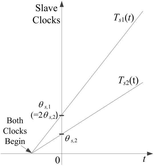
Figure 1: Illustration of the ratio of phase differences (w. r. t. the ideal reference clock) when dual slave clocks begin simultaneously.

Now consider the equations (5) and (6) of [1] describing a relationship between the times of slave clocks when the $i$-th Sync message is received:

$$T_{s1}.i {=} 2\left(1+\epsilon\right)\left(T_{m}.i+D_{m2s}\right)+\theta+\phi_{1,i}$$

$$T_{s2}.i {=} \left(1+\epsilon\right)\left(T_{m}.i+D_{m2s}\right)+\theta+\phi_{2,i},$$

where $D_{m2s}$ is the master-to-slave delay, $\theta$ is a common offset of the slave clocks, and $\phi_{1,i}$ and $\phi_{2,i}$ are random jitters of slave clock 1 and 2 within a period, respectively. We can see that, except for the noise components (i.e., $\phi_{1,i}$ and $\phi_{2,i}$ representing clock jitters), (4) and (5) are generalized expressions (i.e., at any time instant) for time relationship between the master and the slave clocks.

Chin and Chen argue that, because a single signal drives both the clocks as shown in Fig. 3 of [1], they have the same offset (i.e., $\theta$) with respect to the master clock. This, however, is not the case in general; from (7) and (8), we obtain the condition for the slave clocks to have a common offset with respect to the master clock (i.e., $\tilde{\theta}_{s,1}=\tilde{\theta}_{s,2}$) as follows:

$$\theta_{s,1}-\theta_{s,2}=\left(1+\epsilon\right)\theta_{m}.$$ (9)

As we discussed with (6)–(8), the number of parameters of the left-hand side of (9) can be reduced to one (e.g., $\theta_{s,2}$ when $\theta_{s,1}/\theta_{s,2}=2$), but at the the right-hand side, both $\epsilon$ and $\theta_{m}$ are unknown at the slave and parameters to be estimated. In other words, for the equations (5) and (6) of [1] to be valid, not only the value of $\theta_{s,2}$ (or $\theta_{s,1}$) but also the values of $\epsilon$ and $\theta_{m}$ should be known at the slave, which verifies that Chin and Chen’s formulation of multi-parameter estimation is invalid.

Note that in case of $\theta_{s,1}=2\theta_{s,2}$ (i.e., both the slave clocks begin (or reset) at the same time), the times of slave clocks should meet the following condition (again, ignoring random noise components for simplicity):

$$T_{s1}(T_{m})=2T_{s2}(T_{m}).$$ (10)

In such a case the equations (5) and (6) of [1] should be rewritten as

$$T_{s1}.i {=} 2\left\{\left(1+\epsilon\right)\left(T_{m}.i+D_{m2s}\right)+\theta\right\}+\phi_{1,i}$$ (11)

$$T_{s2}.i {=} \left(1+\epsilon\right)\left(T_{m}.i+D_{m2s}\right)+\theta+\phi_{2,i}$$ (12)

Unlike the original equations of [1], (11) and (12) cannot be manipulated to separate the delay ($D_{m2s}$) from the clock offset ($\theta$) or vice versa, which invalidates the resulting maximum likelihood (ML) estimates in [1].

Note that, in practical applications like clock synchronization in wireless sensor networks (WSNs), the best one can do with these equations is the estimation of the clock skew and the clock offset assuming that $D_{m2s}$ is negligible and that $\epsilon\approx 0$ as suggested in [2].

References

- [1] W.-L. Chin and S.-G. Chen, “IEEE 1588 clock synchronization using dual slave clocks in a slave,” IEEE Commun. Lett., vol. 13, no. 6, pp. 456–458, Jun. 2009.
- [2] Y.-C. Wu, Q. Chaudhari, and E. Serpedin, “Clock synchronization of wireless sensor networks,” IEEE Signal Process. Mag., vol. 28, no. 1, pp. 124–138, 2011.