Applications and identification of surface correlations

Abstract

We compare theoretical, experimental, and computational approaches to random rough surfaces. The aim is to produce rough surfaces with desirable correlations and to analyze the correlation functions extracted from the surface profiles. Physical applications include ultracold neutrons in a rough waveguide, lateral electronic transport, and scattering of longwave particles and waves. Results provide guidance on how to deal with experimental and computational data on rough surfaces. A supplemental goal is to optimize the neutron waveguide for GRANIT experiments. The measured correlators are identified by fitting functions or by direct spectral analysis. The results are used to compare the calculated observables with theoretical values. Because of fluctuations, the fitting procedures lead to inaccurate physical results even if the quality of the fit is very good unless one guesses the right shape of the fitting function. Reliable extraction of the correlation function from the measured surface profile seems virtually impossible without independent information on the structure of the correlation function. Direct spectral analysis of raw data rarely works better than the use of a ”wrong” fitting function. Analysis of surfaces with a large correlation radius is hindered by the presence of domains and interdomain correlations.

year number number identifier Date text]date LABEL:FirstPage1 LABEL:LastPage#1

I Introduction

Progress in material science, nanofabrication and related technologies expands the range of physical systems in which scattering by surface and interface roughness is the dominant scattering channel. Such systems are studied by different theoretical, experimental, and computational techniques, all of which, in principle, should use a more or less common language and converge to identical results. Below we try to answer the question how to bridge the gap between these techniques. Our applied goal is to find ways to prepare a random rough surface with desirable physical properties.

We are interested in surfaces with slight random roughness for which the observables are quadratic in roughness. Theoretical expressions for the physical observables, such as, for example, transport coefficients, should explicitly contain the geometrical and statistical parameters of surface roughness. These parameters are routinely introduced (see, e.g., Ref. q2 and references therein) by the binary roughness (auto-)correlation function $\zeta\left(x\right),$ which is usually characterized by an average amplitude of inhomogeneities $\ell$ and a single correlation radius of inhomogeneities $R$,

$$\zeta\left(x\right)=\ell^{2}\varphi\left(x/R\right),\ \varphi\left(0\right)=1.$$ (1)

An equivalent description uses the roughness structure function, $S\left(x\right)=\ell^{2}\left(1-\varphi\left(x\right)\right)$. A brief review of alternative approaches to roughness can be found in Ref. bernasek1 . For applications, the Fourier image of the correlation function $\left(\ref{i1}\right)$ (the so-called power spectrum of surface roughness),

$$\zeta\left(q\right)=\ell^{2}\psi\left(qR\right),$$ (2)

is often more important than the correlation function itself (here $q$ is an appropriate conjugate for $x;$ in 1D there could be an extra coefficient $\sqrt{2\pi}R$, in 2D - just $R^{2}$). The use of multiparameter descriptors instead of Eqs. $\left(\ref{i1}\right),\left(\ref{ii1}\right)$ could provide additional fitting parameters, but usually does not clarify the physics.

The form of the roughness correlation function for real surfaces cannot be predicted theoretically except for a few exactly solvable models of surface interaction which may or may not correspond to reality. Even the simplest models rarely lead to simple explicit expressions for the correlation functions. One can also try to establish classes of universality for roughening and to find the roughening or fractal exponents (for recent examples see Refs. fracture1 ; fracture2 ; fracture3 and references therein). In theoretical calculations the correlation function is usually assumed to be known leaving its determination to experiment or numerical modeling.

These sources are often inconclusive and the theoretical evaluation of observables is performed using some ad hoc correlation function. The variety of Gaussian, exponential, or power law correlators are used almost at will despite the evidence that the choice of the correlation functions with similar correlation parameters but of different functional forms can lead to very different physical results (see, e.g., Refs. q2 ; fer1 ; munoz1 ; pon1 ). All this degrades the application of theoretical results to real surfaces.

Thus the questions are whether it is possible to extract an accurate correlation function from experiment and whether it is possible to create a random rough surface with a predetermined roughness correlation function. We will start from the former question and later give a physical example for which the latter question is indeed crucial.

There are two types of experiments which can provide information on the surface correlation function: scattering of particles or waves by the rough surface and direct measurements of the surface profile. The intensity of waves scattered from a rough surface is directly described by the power spectrum of the correlation function $\left(\ref{ii1}\right)$ q2 , but the accuracy of measurements is high only in limited ranges of wave vectors and angles.

The second type of experiment seems more promising since one can easily extract the correlation function $\zeta^{\exp}$ from precise scanning measurements of the surface profiles, such as, for example, STM or AFM. The difficulty here lies in proper identification of the raw data on $\zeta^{\exp}$. This extracted discrete correlation function $\zeta^{\exp}$ inevitably exhibits noticeable noise, especially if the scanned area is not very large, and cannot be unambiguously identified with some simple functional form of $\zeta\left(x\right)$, Eq. $\left(\ref{i1}\right)$. There are two ways of dealing with these difficulties: either compare the extracted correlator $\zeta^{\exp}$ with some preconceived fitting function $\zeta^{fit}\left(x\right)$ and get the correlation parameters from the best fit or feed the the extracted raw correlation function $\zeta^{\exp}$ directly into the theoretical equations for observables. Below we analyze the limitations of both approaches.

The experimental difficulties of extracting an accurate surface correlator multiply when one deals with an atomic-scale roughness, even if one disregards the issue of the accuracy of the data on the surface profile related, for example, to the tip profile stm1 or the step size munoz4 . Some requirements on accuracy of profile measurements for reliable extraction of the correlation parameters are discussed in Refs. ogilvy2 ; shikin1 . It is not even clear to what extent the theoretical methods using the correlation function of surface roughness can be applied to random inhomogeneities on atomically-smooth crystal surfaces.

The potential shortcomings of the first approach are obvious: the correlation parameters which are extracted from $\zeta^{\exp}$ in this way, depend on an ad hoc choice of the fitting function. Fitting of the STM data on $\zeta^{\exp}\left(x\right)$ to correlation functions $\zeta^{fit}\left(x\right)$ of different functional forms could yield vastly different values of the correlation parameters such as the correlation radii $R$ (for recent experimental examples see, e.g., Refs. munoz1 ; munoz2 ). This can become a real problem when the step size in scanning microscopy is comparable to the correlation radius of roughness: according to the estimates q2 , to resolve the shape of the correlation peak one needs about ten points within the peak. As we will see, even the increase in the sample size does not necessarily help. In the end, using a preconceived correlation function is especially dangerous in two limiting cases when the correlation radius $R$ is comparable to the scanning step or when $R$ and, therefore, the size of inhomogeneities, is large. However, as we will see below, the use of the raw experimental data on $\zeta^{\exp}$ can often be more dangerous than the risk of using the wrong fitting function.

But how can one evaluate the reliability of identifying the correlation function extracted from precise scanning measurements of the surface profile? As we will see, the statistical quality of a fit to some fitting function is not the answer.

The main issue is that we cannot fabricate a surface with a known correlation function to serve as a reference to check against the extracted correlator. What we can do instead is to computationally generate a surface with a given correlation function, scan this surface, and analyze the extracted correlators. The knowledge of the exact correlation function will allow us to judge the quality of identification not by statistical properties of the fits, but by how well the physical observables are reproduced. The identification issues for real and computationally generated surfaces are more or less the same goodnick1 ; shikin1 ; palas1 ; munoz2 and our results should provide a roadmap for dealing with experimental data. This will also allow us to accomplish our second applied goal: to design a random surface with desirable correlation properties which in the case of a reasonable physical scale can be reproduced experimentally (see below).

We start (Section II) from two computational procedures for generating random rough surfaces with known correlation functions. The first procedure produces a random rough surface with any predetermined correlation function and is suitable for larger scale roughness. The second one relies on model Hamiltonians. It provides surfaces with discretized profiles, more appropriate for atomic-scale roughness, but with a limited number of correlators. Which of the procedures is preferable depends on the physical circumstances.

In Section III we briefly describe physical applications which we use to test the results. For clarity, we chose the applications for which the roughness contribution to the observables collapses into a single constant. This ensures effective and unambiguous evaluation of the quality of the data and our methods. The first of these applications, namely, quantized ultracold neutrons in rough waveguides, is essentially a one dimensional (1D) application with a large spatial scale of roughness (the typical scale is 6 $\mathrm{\mu m}$). Here we also have a practical goal: designing the best rough waveguide for experiments in GRANIT installation (ILL, Grenoble) by optimizing the waveguide roughness. Transferring the generated profile onto the real mirror seems to be technically feasible because of a large spatial scale of roughness and is by far preferable to the current procedure of introducing the uncontrolled roughness (random scratching of the mirror). Our second application is more traditional and deals with the conductivity of two dimensional (2D) ultrathin films in quantum size effect (QSE) conditions and, more generally, with scattering of longwave particles and waves by rough surfaces.

In Section IV we analyze random surface profiles generated using the methods of Section II. We extract the correlation functions from these profiles and try to identify them by fitting to different types of the fitting functions using the same procedures used in analyzing the results of the scanning microscopy measurements with a fixed step. The results of the fits are then used to calculate the observables for the applications from Section III. The purpose here is to find out what kind or errors are introduced by ad hoc assumptions about the shapes of the fitting functions when analyzing experimental and numerical data on surface profiles. Since in this case we know the ”true” correlation functions, we have an excellent criterion to compare the errors. We will see that the quality of the fit, which is described by the standard deviation $\sigma$ between $\zeta^{\exp}\left(x\right)$ and the fitting function $\zeta^{fit}\left(x\right)$ does not translate into the quality of the physical results unless the fitting function $\ell^{2}\varphi^{fit}\left(x/R\right)$ has the right functional form which is, unfortunately, unknown in most experiments with real surfaces. In many cases the physical results turn out even worse if one tries to input the raw experimental data on $\zeta^{\exp}$ directly into the calculations instead of risking to make a wrong guess about the functional form of the fitting function $\varphi^{fit}\left(x/R\right)$. The results are summarized in Section V.

II Generation of rough surfaces

In this Section we briefly describe two numerical methods for generating random rough surfaces with predetermined correlation functions. A short review of alternative approaches is given, for example, in Ref. tribology1 . Some of the earlier work in this direction can be found in Refs. ogilvy2 ; navarini1 .

II.1 Surfaces with arbitrary correlation functions

In this subsection we generate random surfaces with an arbitrary predetermined correlation function of surface roughness without paying attention to discretization of the amplitudes on atomic scale. In this sense, we will be generating macroscopic or ”classical” roughness with the only constraint that the profiles are described by the smooth functions. This is appropriate for rather thick films or waveguides and for particles/waves with relatively large wavelengths.

A random rough profile $y\left(x\right)$ can be generated numerically using some distribution function $P\left(y\right)$. The usual choice is the Gaussian distribution,

$$P\left(y\right)=\frac{1}{\sqrt{2\pi}}\exp\left(-y^{2}/2\right),$$ (3)

(see Ref. q2 and references therein). The simple distribution $P\left(y\right)$ of the type $\left(\ref{g1}\right)$ leads to an uncorrelated roughness, $\zeta\left(x\right)\propto\delta\left(x\right)$ (white noise). To produce meaningful desirable binary correlations $\zeta\left(x\right)$,

$$\zeta\left(x\right)=\left\langle y\left(x^{\prime}\right)y\left(x^{\prime}+x\right)\right\rangle_{x^{\prime}}\equiv\frac{1}{L}\int y\left(x^{\prime}\right)y\left(x^{\prime}+x\right)dx^{\prime},$$ (4)

one requires a more complicated distribution $P\left[y\left(x\right)\right]$ than the straightforward distribution $\left(\ref{g1}\right)$ which is embedded in the generators of random numbers.

The first step is discretizing the surface into a large number segments,

$$y\left(x\right)\rightarrow y_{i}=y\left(x_{i}\right),i=1,2,...,N$$ (5)

and, if necessary, smoothing the resulting profile after the computations are done. One way to proceed is to generate the surface with a generalized Gaussian probability distribution,

$$P\left[\overrightarrow{y}\right]=C\exp\left(-\frac{1}{2}\overrightarrow{y}\cdot\widehat{G}\overrightarrow{y}\right),\,\overrightarrow{y}=\left(y_{1},y_{2},...,y_{N}\right),$$ (6)

with some matrix $\widehat{G}$. The choice of $\widehat{G}$ in $\left(\ref{g3}\right)$ should provide the desired binary correlation function of surface roughness

$$\zeta\left(x\right)\rightarrow\zeta_{ik}=\zeta\left(i-k\right)=\left\langle y_{i}y_{k}\right\rangle=\int y_{i}y_{k}P\left[\overrightarrow{y}\right]d\overrightarrow{y}.$$ (7)

Here $C$ is the normalization constant defined by the equation

$$1=C\int\exp\left(-\frac{1}{2}\overrightarrow{y}\cdot\widehat{G}\overrightarrow{y}\right)d\overrightarrow{y}.$$ (8)

If one rotates the vector $\overrightarrow{y}$,

$$\overrightarrow{y}=\widehat{A}\overrightarrow{g},\,\overrightarrow{g}=\widehat{A}^{-1}\overrightarrow{y},$$ (9)

in such a way as to diagonalize the quadratic form $\overrightarrow{y}\cdot\widehat{G}\overrightarrow{y}$,

$$-\frac{1}{2}\overrightarrow{y}\cdot\widehat{G}\overrightarrow{y} =-\frac{1}{2}\widehat{A}\overrightarrow{g}\cdot\widehat{G}\widehat{A}\overrightarrow{g}=-\frac{1}{2}\overrightarrow{g}\cdot\widehat{A^{T}}\widehat{G}\widehat{A}\overrightarrow{g},$$ (10)

$$\widehat{A^{T}}\widehat{G}\widehat{A} =\widehat{I}\equiv\delta_{ik},\,$$ (11)

the probability distribution $\left(\ref{g3}\right)$ (including the Jacobian) becomes

$$P\left[\overrightarrow{y}\right]d\overrightarrow{y}\rightarrow P\left[\overrightarrow{g}\right]d\overrightarrow{g}=\frac{1}{\left(2\pi\right)^{N/2}}\exp\left(-\frac{1}{2}\sum_{i=1}^{N}g_{i}^{2}\right)d\overrightarrow{g}$$ (12)

meaning that all $g_{i}$ are statistically independent,

$$\left\langle g_{i}g_{k}\right\rangle=\int g_{i}g_{k}P\left[\overrightarrow{g}\right]d\overrightarrow{g}=\delta_{ik}\text{.}$$ (13)

The coefficient in Eq. $\left(\ref{g9}\right)$, together with the transformation Jacobian, gives the normalization coefficient $C$ in Eqs. $\left(\ref{g3}\right),\left(\ref{g5}\right)$. Then the roughness correlation function $\widehat{\zeta}=\left\langle y_{i}y_{k}\right\rangle$ acquires the form

$$\widehat{\zeta} =\int y_{i}y_{k}P\left[\overrightarrow{y}\right]d\overrightarrow{y}=\int A_{il}g_{l}A_{km}g_{m}P\left[\overrightarrow{g}\right]d\overrightarrow{g}$$ (14)

$$=A_{il}A_{km}\delta_{lm}=\left(G^{-1}\right)_{ik}.$$

(the last equation is based on Eq. $\left(\ref{g8}\right)$). Therefore, numerically the problem requires inverting the ”desirable” matrix $\widehat{\zeta}$, $\widehat{G}=\widehat{\zeta}^{-1}$, and computing the rotation matrix $\widehat{A}$. For real symmetric matrices, the rotation matrix $\widehat{A}$, according to Eq. $\left(\ref{g11}\right)$, is

$$\widehat{A}=\widehat{\zeta}^{1/2}\text{.}$$ (15)

Summarizing, generating a random rough surface with a desirable correlation function of surface roughness $\zeta\left(x\right)$ $\left(\ref{g2}\right)$ reduces to generating a set of random uncorrelated numbers $\overrightarrow{g}$ for a simple Gaussian distribution $\left(\ref{g1}\right)$ and rotating this vector using the rotation operator $\widehat{A}$ $\left(\ref{g12}\right)$. Computationally, this is a straightforward task. The only limitations on the surface size, as measured in terms of step sizes $b=\Delta x=x_{i+1}-x_{i}$, are computational resources required to perform the operation $\left(\ref{g12}\right)$ for large matrices $\widehat{\zeta}$. Obviously, this limitation is much more important for two dimensional ($\mathrm{2D}$) surfaces than for one dimensional ($\mathrm{1D}$) ones: in addition to a size explosion in the $\mathrm{2D}$ case, the matrices for the $\mathrm{2D}$ surfaces loose their almost diagonal structure even for very steep correlation functions.

The above procedure is straightforward in $\mathrm{1D}$. Expanding it to $\mathrm{2D}$ surfaces can be done in one of two ways. In principle, one can modify the procedure by designating the raw and rotated profiles $g$ and $y$ not as vectors but as $\mathrm{2D}$ arrays and considering the rotation operator as a 4-component tensor. We preferred instead to make a flat file out of the $\mathrm{2D}$ surface profile and redefine the surface correlator using this flat file. After the rotation, the points of the newly created flat file were projected back onto the surface grid.

There is a certain ambiguity in the computation of the averages $\zeta_{ik}=\zeta\left(i-k\right)=\left\langle y_{i}y_{k}\right\rangle$ in samples of finite size (finite $N$). In a $\mathrm{1D}$ case, one cannot extend evaluation of $\zeta\left(s\right)$ beyond $s=N/2$ without loosing accuracy even if one introduces a periodic boundary condition. The same is true when extracting the correlation function $\zeta^{\exp}\left(s\right)$ from the scanning microscopy data on the surface profile.

In a $2D$ system the loss of data points is worse. If the sample is large enough, one can limit oneself to using $N/4$ (one quadrant of the surface) for a straightforward calculation of the correlator up to the distances $\sqrt{N}/2$. If the sample size $L=\sqrt{N}$ is an issue, which is usually the case since the required processing power is determined by $N$ and not $L$, one can extend the computation to approximately $N/2$ points but should take special care to avoid double-counting of the correlations.

This technique allowed us to generate a rough surface with an arbitrary correlation function of roughness. In numerical examples below we reproduce three most popular types of the correlators, namely, the Gaussian,

$$\varphi_{G}=\exp\left(-x^{2}/2R^{2}\right),$$ (16)

exponential,

$$\varphi_{E}=\exp\left(-x/R\right),$$ (17)

and power law

$$\varphi_{PL}=\frac{1}{\left(1+x^{2}\right)^{3/2}}$$ (18)

correlation functions. The same correlation functions will be used as fitting functions when probing the surfaces. All numerical parameters, extracted with the help of these correlators, will carry the same indices $G,E,$ and $PL$. Note that our particular power law correlator $\left(\ref{pl1}\right)$ has an exponential power spectrum and vice versa.

Each physical system has its own spatial scale $l_{0}$. These scales for different systems can differ from each other by orders of magnitude. It is convenient to measure length parameters of each correlator in units of its own physically meaningful scale $l_{0}$ leaving the definition of $l_{0}$ to the underlying physical systems. We have three length parameters: the average amplitude of surface roughness $\eta=\ell/l_{0},$ the correlation radius of roughness $r=R/l_{0}$, and the step (grid) size $b=\Delta s/l_{0}=x_{i+1}-x_{i}$, Eq. $\left(\ref{g9}\right).$ Since the square of the amplitude of surface inhomogeneities $\ell$ enters most of the physical results as a simple scaling parameter, in all illustrations we assume, unless mentioned otherwise, that $\eta=\ell/l_{0}=1$ and assign other values to $\eta$ only when the physical situation requires this. Therefore, in graphical illustrations below the amplitude of profile inhomogeneities can be arbitrarily compressed resulting in smoother profiles and correlation functions. The values of $b$ and $r$ are not necessarily independent: for example, one can generate the correlation functions with various values of $r$ either by calculating the rotation matrix $\widehat{A}\left(b=1,r\right)$ directly or calculating $\widehat{A}\left(b,r=1\right)$ and then compressing or stretching the generated surface so that get the desired value of $r$. In some situations $b$ is an independent physical parameter. The most obvious example is the step size in the STM-like measurements.

The accuracy with which the generated surface reproduces the desirable correlator $\zeta$ improves with the increase in the number of points $N$. The limit of accessible values of $N$ depends on our ability to compute and use the $N\times N$ matrix $\widehat{A}$, Eq. $\left(\ref{g12}\right)$ (in our examples going to $N$ above five thousand was not practical with easily available resources).

Even with a fixed large number of points $N,$ the standard deviation $\sigma$ between the desirable and generated correlators is not always the right way to look at the quality of the generated rough surfaces. In general, the correlation function consists of two parts: a peak area of the size $r$, which describes the short-range correlations, and a long tail of long-range correlations. Under the usual circumstances, the correlation function is expected to go to zero at large distances. However, the correlation functions for finite size samples inevitably contain long fluctuation-driven tails. The same is true for experiments on restricted scanning areas. As a result, $\sigma$ is determined mostly by these tails of the correlation functions and is not very sensitive to the shape of the peak area. Paradoxically, the larger the size of the sample the less sensitive can $\sigma$ be to the shape of the short-range peak and the rate of decrease of the ”real” correlation function. We will encounter this issue throughout the paper.

On the other hand, the contributions from the peak and tail areas to physical observables for different physical applications enter with different weights: while some of the observables are more sensitive to the short-range correlations from the peak area, the others require more information and, therefore, better accuracy, in the tails. When the peak area is more important, one should have more points inside the peak. The number of such points is given by the ratio of the correlation radius $r$ to the step size $b$, $r/b$. However, a large increase in the number of such points leads to proportional decrease in the number of surface inhomogeneities $Nb/r$ (”clusters” or ”domains”) which one can fit on the generated surface with the fixed overall number of points $N$. This, in turn, suppresses accuracy of the generated correlation tails and increases the value of the overall $\sigma$ which is weighted more heavily towards the tails of the correlation functions. This effect was obvious when we looked at $\sigma$ as a function of $r/b$. As a result, the computer generation of rough surfaces with large correlation radii $r$ requires a dramatic increase in the overall number of points which is difficult to achieve. This also means that reliable computer simulations of theoretically predicted physical effects at very large $r$ are not feasible. For example, we are currently not able to reproduce computationally a new type of quantum size effect in conductivity of ultrathin films, predicted in Ref. pon1 , by generating a thin film with rough surface with very large $r$. We will encounter this issue later on in a slightly different context.

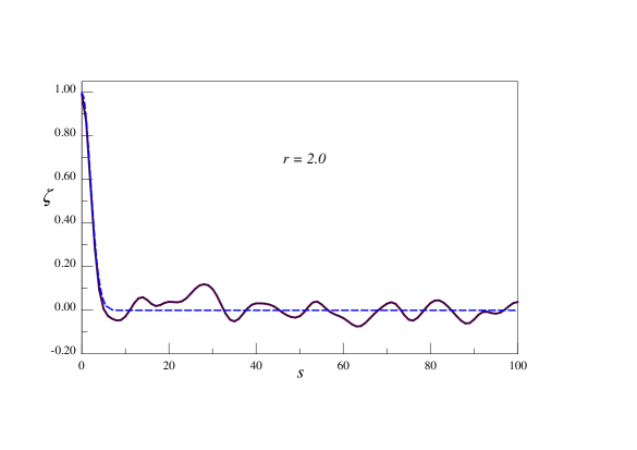
Figure 1: An example of the correlation function (black solid line) for a generated $\mathrm{1D}$ surface which should emulate a surface with Gaussian correlation of inhomogeneities $\zeta\left(x\right)=\exp\left(-x^{2}/8\right)$ (blue dashed line). The total number of points is 2000, the average amplitude of roughness $\eta=\ell/l_{0}=1$, the correlation radius $r=R/l_{0}=2.$

In Figure $1$ we present the initial part of the correlation function (black solid line) for the generated $\mathrm{1D}$ surface profile which should emulate a surface with the Gaussian correlation of inhomogeneities $\zeta\left(x\right)=\exp\left(-x^{2}/8\right)$ (dashed blue line). The total number of points is $N=2000$, the average amplitude of roughness $\eta=\ell/l_{0}=1$, the correlation radius $r=R/l_{0}=2.$ The long oscillating tail in the correlation function reflects fluctuations.

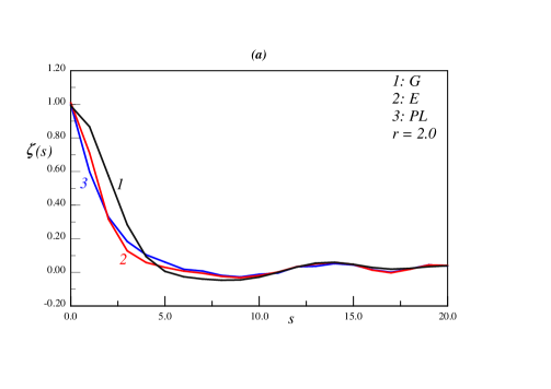
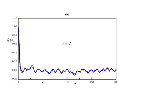
Figure 2:  Correlation functions for $\mathrm{1D}$ generated surface profiles which should emulate the Gaussian (black; curve 1), exponential (red; curve 2), and PL (blue; curve 3) correlation functions. In the peak area (Figure $2a$) the differences are very pronounced, but the fluctuation-driven tails (Figure $2b$) are almost identical. All three computations started from the same set of $N=2000$ random numbers.

For comparison, in Figure $2$ we plotted together correlation functions which should reproduce the Gaussian $\zeta\left(x\right)=\exp\left(-x^{2}/8\right)$ (curve 1; black), exponential $\zeta\left(x\right)=\exp\left(-x/4\right)$ (curve 2; red), and power law $\zeta\left(x\right)=1/\left(1+x^{2}/4\right)^{3/2}$ (curve 3; blue) correlation functions with $N=2000$, $\eta=\ell/l_{0}=1,$ and $r=R/l_{0}=2.$ In all three cases the generation started from the same set of random numbers $\overrightarrow{g}$. It is clear that in the peak area (Figure $2a$) the correlations are different, but in the tail area (Figure $2b$: the same functions $\zeta\left(s\right)$ as in Figure $2a$ extended to $s=200$) all three curves look the same. As a result, the quality of reproducing the desired correlation function is the same if measured by $\sigma$ which is heavily weighted towards the fluctuation-driven tail area.

As expected, the value of the standard deviation $\sigma$ between generated and exact correlation functions decreases with increasing surface size $N$ as $\sqrt{2/N}$ (Figure 3).

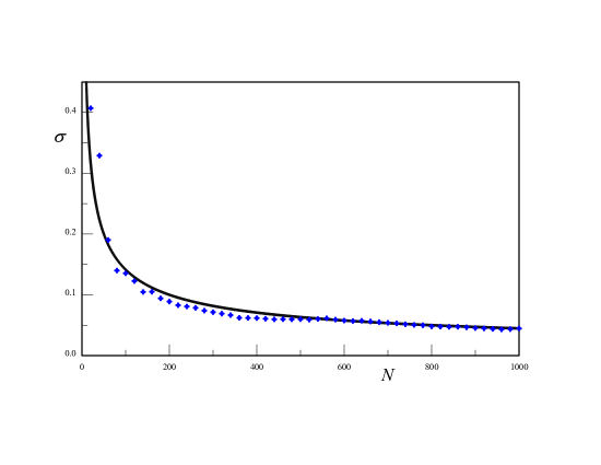
Figure 3: Dependence of the standard deviation $\sigma$ between generated and exact correlation functions on the sample size $N$. The solid line is $\sqrt{2/N}$. The generated roughness is supposed to have Gaussian correlations with $r=2$.

Generation of $\mathrm{2D}$ roughness by this method requires more computational resources. We were not able to routinely proceed for surfaces $L\times L$ with size $L$ well above $70$ when the size of the rotation matrix $\widehat{A}$ exceeds $4900\times 4900$; computations beyond that required special efforts. An example of a correlation function for a generated $\mathrm{2D}$ rough surface is given in Figures 4. The roughness correlations were supposed to emulate isotropic Gaussian correlations with $r=2$, $\zeta\left(s\right)=\exp\left(-s^{2}/8\right)$. Figure 4$a$ shows the $\mathrm{2D}$ correlation function $\zeta\left(x,y\right)$ for this surface. The anisotropy of the extracted correlation function is well pronounced. Similar anisotropy of the extracted correlator is quite pronounced in STM experiments as well (see, for example, Ref. munoz4 ). After averaging over the angles, this correlation function becomes $\zeta\left(s\right)$ in Figure 4$b$ (blue curve; the black curve gives the emulated Gaussian correlator $\exp\left(-s^{2}/8\right)$).

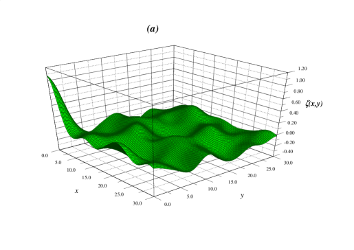
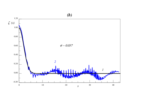
Figure 4: An example of a $\mathrm{2D}$ rough surface of the size $60\times 60$. The roughness emulates isotropic Gaussian correlations with $r=2$, $\zeta\left(s\right)=\exp\left(-s^{2}/8\right)$ (black line 1 in Figure 4$b$). ($a$) $2D$ correlation function $\zeta\left(x,y\right)$ ($b$) The correlation function $\zeta\left(s\right)$ after averaging over the angles (line 2; blue).

The standard deviation between the two curves in Figure 4$b$ is surprisingly small, $\sigma\sim 0.057$, though visually the generated correlation function $\zeta\left(r\right)$ looks very volatile while the 2D function $\zeta\left(x,y\right)$ is smooth. The reason for this volatility is quite obvious: the nearby points in $\zeta\left(r\right)$ correspond very different orientations in $\zeta\left(x,y\right).$ With increasing sample size $L$ the volatility actually increases because the density of data points in $\zeta\left(r\right)$, each of which represent different directions, goes up at large $r$. The volatility becomes so strong that the flattened correlation function becomes unstable and practically useless for data analysis and one should deal with the anisotropic $\zeta\left(x,y\right)$ directly (see Section IV).

Another difficulty, which, though common to both $\mathrm{1D}$ and $\mathrm{2D}$ surfaces, is exacerbated in the $\mathrm{2D}$ case, concerns surfaces with long range correlations of inhomogeneities (large $r$). The large value of $r$ means that the surface is covered by large size inhomogeneities (domains). The larger the value of $r$, the smaller the number of inhomogeneities for the samples of the same linear size $L$. The correlations of particles within each inhomogeneity are responsible for the central peak of the radius $r$ in the correlation function $\zeta\left(r\right)$. However, there are noticeable non-zero correlations between the particles from different inhomogeneities which are due not to some aligning physical forces, but simply to geometrical factors arising from the large size of inhomogeneities. These non-zero interdomain correlations manifest themselves as smaller secondary peaks of the radius $r$ at positions that correspond to the integer numbers of average distances between the domains. If the sample is large enough to contain a very large number of such domains, these secondary peaks are washed out. The washing out of these peaks is determined not by the total number of data points in the sample $N$, which is proportional to $L$ or $L^{2}$ depending on dimensionality, but by the ratio $N/N_{i}$ where $N_{i}$ is the number of particles in a typical domain. If the number $N$ is not very big or the inhomogeneity clusters $N_{i}$ are large, these secondary peaks survive and $\zeta\left(r\right)$ looks as if the system has an additional, larger correlation radius $R_{2}$. The situation is worse in the 2D case in which the number of particles in a domain $N_{i}$ grows with $r$ as $r^{2}$. If one plots the set of correlators for the generated surface with increasing $r$, one will see a widening central peak and tails with more and more distinct secondary correlation peaks. In our typical $\mathrm{1D}$ examples with $N=2000$ one cannot proceed with $r$ well above $10$ without the tails loosing any relationship to the physical forces and starting to reflect purely geometrical interdomain correlations. This explains why it is so difficult to generate rough surfaces with large $r$.

II.2 Surfaces with discrete (integer) amplitudes of roughness

Above we treated rough surfaces as 1D or 2D objects that are described by smooth functions. This can be easily justified when the natural physical scale of the system $l_{0}$ is much larger than the atomic size $a$, $l_{0}\gg a$, as in our neutron example in which $l_{0}\simeq 6$ $\mu\mathrm{m}$ (see Section IIIA below). This is a good approximation for systems with macroscopic roughness and/or longwave particles. In the case of electrons in ultrathin metal films the amplitudes of inhomogeneities have atomic scale and the situation is different. The approach should depend on whether one deals with atomically rough or atomically smooth surfaces. In the former case, such as, for example, for amorphous films, the theoretical description via the correlation function might still work though the correlators should be discretized in order to account for discrete nature of atomic-size steps in scanning measurements or computer models. In the latter case, the rough surfaces can be understood as perfect crystal faces with roughness introduced by randomly distributed adatoms/vacancies and steps with kinks. If this is the case, then the roughness profile is described by an integer number of defects of the atomic height $a$ which now becomes the only scale of the problem. Then the use of continuous correlators for computer modeling and STM data should be revisited even if one ignores the obvious angular anisotropy. For example, the small value of the amplitude of the correlation function $\ell$ as in experiment munoz2 might mean that either the amplitude of roughness is indeed small or that there is simply very few surface defects. In the latter case the meaning of the roughness correlation radius can itself become murky.

The generation of rough surfaces with discretization of amplitudes on atomic level cannot be done using a generic procedure of Section II: the rotation matrix $\widehat{A}$, Eqs. $\left(\ref{g6}\right),\left(\ref{g12}\right),$ is determined solely by the desirable correlator $\widehat{\zeta}$ and the generated surface profile $y_{i}$ does not reduce to a set of integer numbers in terms of $a$ even if before the rotation the starting values of $g_{i}$ were integer. In general, the best we can do with this procedure is to generate the set of $y_{i}$ and then round the values of $y_{i}$ to the nearest integer number $\tilde{y}_{i}$. This, of course, changes the correlation function. The results of this approach are illustrated in Figure 5. In this Figure we used the method of Section IIA to generate the rough surface which emulates the exponential correlator $\zeta\left(i-k\right)=4\exp\left(-\left|i-k\right|/2\right)$ and then rounded the data points $y_{i}$ to the nearest integer number $\tilde{y}_{i}$. The black curve in the Figure is the initial theoretical correlator, the red line is the correlator $\zeta\left(\left|i-k\right|\right)=\left\langle y_{i}y_{k}\right\rangle$ of the generated rough surface, and the blue line is the correlator $\widetilde{\zeta}\left(\left|i-k\right|\right)=\left\langle\tilde{y}_{i}\tilde{y}_{k}\right\rangle$ after the discretization of the surface profile $y_{i}$ to integer numbers. As one can see, this procedure can work at best qualitatively.

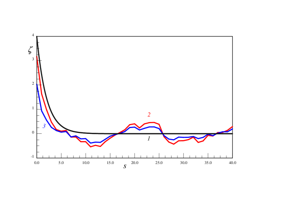
Figure 5: Correlation function for a generated surface emulating $\zeta\left(i-k\right)=4\exp\left(-\left|i-k\right|/2\right)$ (line 1; black) after rounding the profile data points $y_{i}$ to the nearest integer number $\overline{y}_{i}$. Line 2 (red): the generated raw correlator $\zeta\left(\left|i-k\right|\right)=\left\langle y_{i}y_{k}\right\rangle$, line 3 (blue): the correlator for the discretized surface $\left\langle\overline{y}_{i}\overline{y}_{k}\right\rangle$.

It might be impossible to computationally emulate a random rough surface with an integer profile $\tilde{y}_{i}$ with an arbitrary predetermined correlation function $\widehat{\zeta}\left(i-k\right)=\left\langle\tilde{y}_{i}\tilde{y}_{k}\right\rangle$ except, of course, for ”classical” surfaces with very large amplitude of roughness $\ell$, $a\ll\ell\ll R$. However, several specific correlators can still be generated based on spin lattice models with various Hamiltonians. This might help in extracting the proper correlation functions from experimental data on the surface profile based on realistic assumptions on the interaction of the surface defects. This can also help to guess which correlation functions to use in theoretical calculations. Needless to say, many of the lattice models produce the correlation functions which are exponential at large distances and have complicated, often analytically unresolved structure in the peak area.

Unfortunately, the universe of the correlation functions which are accessible in this way is limited by the number of known exactly solvable lattice models, mostly in 1D, some of which may have little resemblance to real surfaces. It is even unclear whether there are any restrictions on allowed forms of the correlation functions. In 2D even the simplest models, such as the Ising model, lead to the correlation functions for which we do not have explicit analytical expressions making them virtually useless for our purposes.

There are a couple of additional practical difficulties for using this approach. First, when the correlation radius $R$ is comparable to or smaller than the lattice constant $a$, the reliable extraction of $R$ or the shape of the peak in the correlator from either computer generated surface or STM data still remains impossible. In the opposite case, when $R$ is large, the computational requirements rapidly increase because of the large size inhomogeneities (domains). The latter requires not only going to much large sample sizes but also an increase in computing time because of a slowdown in convergence.

The simplest example is, of course, the ferromagnetic Ising lattice $y_{i}=\pm 1$ where the correlation function is determined by the attractive coupling constant $J$ in the Hamiltonian (or, what is the same, by the Boltzmann factors $\exp\left(\pm 2J/kT\right)$). In the 1D case the correlation function is exponential,

$$\zeta_{E}\left(x\right)=\eta^{2}\exp\left(-x/r\right),\ r=\frac{1}{2}\exp\left(2J/kT\right).$$ (19)

The correlation function for the 2D Ising model, though known in principle, Ref. johnson1 , is described by a set of complicated equations involving elliptical integrals.

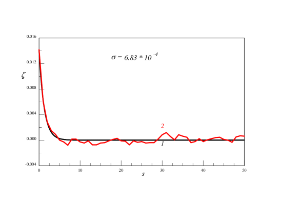
Figure 6: An example of the correlation function for a $\mathrm{1D}$ rough surface $y\left(x\right)$ and its correlation function $\zeta\left(s\right)$ generated using the Ising model (red line 2). The parameters in the correlation function $r=1.19$ and $\eta=0.119$; black line 1 is given by Eq. $\left(\ref{a1}\right)$ ($\sigma=6.83\times 10^{-4}$).

We performed Monte Carlo simulations of $\mathrm{1D}$ and $\mathrm{2D}$ rough surfaces on the basis of the Ising model. The $\mathrm{1D}$ correlation function $\zeta\left(x\right)$ for the generated surface profile $y\left(x\right)$ is illustrated in Figure 6. In computations we used 1000 positions $x_{i}$ and performed $10^{6}$ Monte Carlo cycles. The correlation function $\zeta\left(s\right)$ (red curve in Figure 6) should emulate function $\left(\ref{a1}\right)$ with $r=R/l_{0}=1.19$ and $\eta=\ell/l_{0}=0.119$ (black curve in the figure) as in the neutron experiments (see below). The standard deviation between the desired and generated correlators is $\sigma=6.83\times 10^{-4}$.

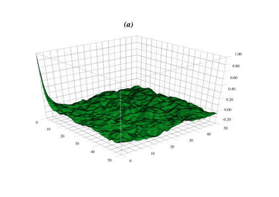
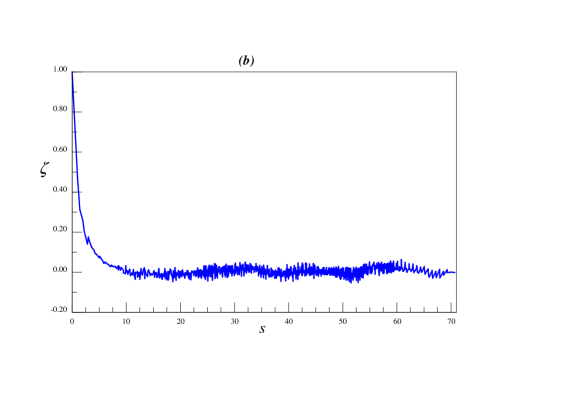
Figure 7: An example of a $\mathrm{2D}$ random rough surface generated using the Ising model at $T=1.2T_{c}$: $a)$ 2D correlation function $b)$ correlation function after averaging over the angles.

Figures 7 illustrate the correlation function for the the surface profile generated using the $\mathrm{2D}$ Ising model at relatively high temperatures, $T/T_{c}=1.2$. At this temperature the relaxation (and computation) times are not very long, domains are small, and the energy equilibrates. On the other hand, the correlation radius already starts to grow and the correlation function should start exhibiting deviations from the pure exponential form. The surface area was $101\times 101$ and we performed $10^{6}$ Metropolis cycles. Figure 7$a$ shows the 2D correlation function for this surface and Figure 7$b$ gives the same correlation function after averaging over the angles. Since the sample size is substantially larger than in Section IIA, the fluctuations are smaller. For the same reason, the volatility of the flattened correlation function is actually higher. A more detailed analysis is presented in Section IV. At high temperatures this approach to generating rough surfaces seems to be better than the one from Section IIA since it allows working with larger samples without involving more computation resources. The situation inverses closer to the transition and below when the relaxation times increase.

III Physical applications

III.1 1D applications: ultracold neutrons in a rough waveguide

Experimental observation of quantization of motion of ultracold neutrons by gravitational field neutron1 was one of the most interesting recent achievements in neutron physics. This is a significant breakthrough in a field with a relatively long theoretical and experimental history going back at least into the late 1960-s; for a review and a list of publications in the field see Ref. nesv2 . The discrete quantum states for neutrons in the Earth gravitational field have extremely low energies with the scale of 1 peV. Though the quantization of motion by a linear field such as gravity is not new by itself breit1 and has been already encountered experimentally in a low-temperature context freed1 , the experimental access to a spectrum of discrete energy states in such a low energy range opens the way for using ultracold neutrons as a very sensitive probe for extremely weak fundamental forces nesv2 ; pdg1 ; prot1 ; grenoble1 .

Currently, the experimental resolution of gravitational states is achieved by sending a horizontal beam of ultracold neutrons between two horizontal mirrors. The top mirror, the ”ceiling”, is intentionally made rough, while the bottom one, the ”floor”, is nearly ideal (the quality of this mirror is such that it can ensure thousands of almost specular consecutive reflections mirror ). The mirrors are reflective only when the normal component of velocity is below a certain threshold; neutrons with velocities above this threshold are absorbed by the mirrors’ material. The beam of ultracold neutrons entering this wave guide contains neutrons with a horizontal velocity noticeably higher than this threshold and a much smaller residual vertical component. The scattering of neutrons by the rough ceiling turns the velocity vector thus increasing its vertical component and leading, eventually, to absorption of the scattered neutrons. The quantization of the vertical motion of neutrons by the Earth gravity field corresponds to the quantization of the amplitude of bounces of neutrons from the floor mirror. In quantum language, the turning of the velocity is equivalent to scattering-driven transitions of neutrons into the higher quantum states. Only the neutrons in the lowest gravitational states with the lowest kinetic energy of vertical motion and, therefore, the lowest amplitudes of bounces, which could not reach the rough ceiling, continue bouncing unimpeded along the floor mirror and are counted by an exit neutron counter.

Recently we demonstrated that the results of such experiments strongly depend on the correlation properties of roughness on the ceiling mirror mauricio1 . The experiments are unique in a sense that the roughness of the ceiling mirror is created artificially. In this application, the spatial scale $l_{0}=\hbar^{2/3}\left(2m^{2}g\right)^{-1/3}\sim 5.871$ $\mu\mathrm{m}$ is the size of the lowest quantum state in the infinite gravitational trap (open geometry without the ceiling); $m$ is the neutron mass. Since this length scale $l_{0}$ is relatively large, it is possible to create the random roughness with optimized correlation properties by computationally generating the required pattern and transferring it onto the real surface. In earlier experiments the roughness was neither optimized nor properly measured. The observation of the surface profile under the microscope yielded the average distance between the nearby maxima and the height of the peaks about 1.19 and 0.119 in units of $l_{0}$. These numbers were accepted as the correlation radius $R$ and the amplitude $\ell$ of surface roughness, $r=R/l_{0}=1.19$ and $\eta=\ell/l_{0}=0.119$, and the roughness was assumed to be Gaussian. Of course, neither of these assumptions could be justified, and the comparison of the theoretical results to the experimental data required adjustments. If the planned new experiments follow the suggestions of this paper, this uncertainty could be eliminated.

An additional attraction of this system is that the geometry of the beam experiment allows one to deal with a practically $\mathrm{1D}$ roughness application in which the motion along the waveguide surface in the direction perpendicular to the beam can be made irrelevant.

In Ref. mauricio1 we demonstrated that, as far as the neutron exit count $N_{e}$ is concerned, all system parameters collapse into a single constant $\Phi$,

$$N_{e}=\sum N_{j}\left(0\right)\exp\left(-\Phi b_{j}\left(h\right)\right),$$ (20)

where $N_{j}\left(0\right)$ are the numbers of neutrons in the in the quantized states $j$ that enter the rough waveguide, $h$ is the average width of the waveguide, and $b_{j}\left(h\right)$ are the values of the wave functions of neutrons in the gravitational states $j$ on the ”ceiling”. Therefore, the problem of computationally optimizing the exit count so that it exhibits the most pronounced step-wise dependence on the waveguide width $h$ reduces to increasing the value of constant $\Phi$ by manipulating the computer-generated correlation functions.

The explicit expression for $\Phi$ via the correlation function $\psi$, Eq. $\left(\ref{i1}\right)$, is mauricio1

$$\Phi\left(\eta,r\right)=A\eta^{2}r\int_{0}^{1}z^{2}\psi\left(y\right)dz$$ (21)

where the constant $A$ is determined by the size and the material of the waveguide (in experiments neutron1 ; nesv2 , $A=92\cdot 10^{-5}\kappa u_{c}^{2}/\pi\chi$), and the variable $y$ in the argument of the power spectrum of the surface roughness $\psi\left(qr\right)$ is

$$y=\frac{1}{\sqrt{\chi}}\left(1-\sqrt{1-z^{2}}\right)\sqrt{u_{c}}r.$$ (22)

Here $u_{c}=U_{c}/mgl_{0}$, $U_{c}$ is the energy threshold for the neutron penetration into material of the waveguide, $\chi=U_{c}/E<1$ is the ratio of this threshold energy to the full kinetic energy of neutrons in the beam (in past experiments $\chi\approx 0.16$), and $\kappa\approx 1$ differs from 1 only because of small variations in the time of flight through the waveguide.

As a result, the computation of $\Phi$, and, therefore, the expected neutron count, for various correlation functions $\psi$ reduces, essentially, to numerical integration in Eq. $\left(\ref{ne2}\right)$. The most important feature here is that, because of the large value of $u_{c}$ (in experiment $u_{c}\sim 10^{5}$), the main contribution to the integral comes from not the whole peak in the power spectrum $\psi\left(qr\right)$, but from the immediate vicinity of its center at $qr=0$. This means that the tails in the computationally generated power spectrum $\psi\left(qr\right)$ are irrelevant, but also that the only issue is to correctly reproduce the vicinity of $\psi\left(0\right)$. However, the closer one gets to $\psi\left(0\right)$, the more important is the tail of the correlation function $\varphi\left(x/r\right)$ at large $x$.

Our recommendation is to generate a random rough profile using the Monte Carlo simulations on the basis of the $1D$ Ising model as described in subsection IIB. In this particular case we prefer this method to the one from Section IIA because it allows easier computation for a large number of points $N$ resulting in smaller fluctuations. Another important benefit is that the transferring the generated pattern to the real mirror is also much simpler because all the inhomogeneities for the Ising profile have the same constant amplitude $\pm\eta$ (Figure $6a$). In this case, the roughness correlation function is exponential $\zeta_{E}$, Eq. $\left(\ref{a1}\right)$, with a simple power-law power spectrum

$$\psi_{E}\left(qr\right)=1/\left(1+q^{2}r^{2}\right)^{3/2}$$ (23)

which yields the following analytical expression for $\Phi$:

$$\Phi_{E}\simeq\frac{1}{3}A\eta^{2}r\,_{2}F_{1}\left(\frac{3}{4},\frac{3}{2},\frac{7}{4},-r\sqrt{u_{c}/\chi}\right)$$ (24)

(see mauricio1 , Eq. (38)).

Improving the experimental outcome, namely observing the well-pronounced quantum steps in neutron count, requires the value of $\Phi$ to be as large as possible. One can get the desirable value of $\Phi$ by simply manipulating values of the correlation radius and the amplitude of surface roughness in computer simulation. The only limitation here is that the amplitude of the mirror roughness $\eta$ should be smaller than both the correlation radius $r$ and the width of the waveguide $h$,

$$\eta\ll r,h.$$ (25)

When making estimates of the optimal values of $\eta$ and $r$, it is convenient to rewrite Eq. $\left(\ref{ne5}\right)$ in the limit $u_{c}\rightarrow\infty$,

$$\Phi_{E}\left(u_{c}\rightarrow\infty\right)\simeq 1.38\frac{A\eta^{2}}{r^{1/2}}\frac{\left(4\chi\right)^{3/4}}{3u_{c}^{3/4}}.$$ (26)

This equation does not have very high accuracy and for final calculations one should still use Eq. $\left(\ref{ne5}\right)$. However, Eq. $\left(\ref{ne6}\right)$ highlights the dependence of $\Phi_{E}$ on $\eta$ and $r$ in a very simple form. Since the value of $\Phi_{E}$, Eq. $\left(\ref{ne6}\right)$, is more sensitive to $\eta$ than to $r$, one should increase $\eta$ as much as possible simultaneously adjusting $r$. The limit is imposed by the width of the waveguide which in experiment comes down to $h\sim 2$. Therefore, the optimal waveguide should have roughness with $r=2$ and the amplitude $\eta<2$. We would not recommend to make $\eta$ much larger than $0.2\div 0.4$ - the ratio $\eta/h$ limits the accuracy of measuring the waveguide width. Still, even this would allow to increase the value of $\Phi$ several times in comparison to what it is assumed to be in previous experiments with an additional benefit of ensuring a perfectly controllable environment. The anticipated value of $\Phi_{E}$ for these parameters is in the $43.5\div 170$ range and one should be able to see well-pronounced quantum steps in neutron count without changing anything else in experiment.

III.2 2D applications: conductivity of ultrathin films and surface scattering

One of the most important applications is ballistic conductivity of ultrathin films with rough surfaces in quantum size effect (QSE) conditions. There are many theoretical approaches to this problem (for a short review of earlier approaches see, for example Ref. arm2 ). The equations relate the $\mathrm{2D}$ conductivity of the films $\sigma$ to the Fourier image (power spectrum) of the correlation function of surface roughness $\zeta\left(\boldsymbol{q}\right)$. Though these equations are more or less transparent, the results, which involve inversion of large matrices, are not. The difficulty arises because of the QSE-driven split of the $\mathrm{3D}$ energy spectrum $\epsilon\left(\mathbf{p}\right)$ into a large set of $\mathrm{2D}$ minibands $\epsilon_{j}\left(\mathbf{q}\right)$ and the corresponding slicing of the Fermi surface. As a result, the transport equation becomes a large set of coupled equations in the miniband index $j$. For the purpose of this paper, namely for analysis of the correlation functions extracted from a numerical or physical experiment, it is better to restrict oneself to the situations in which it is possible to solve this matrix transport equation analytically and get simple explicit expressions for $\sigma$ via $\zeta\left(\boldsymbol{q}\right)$ (see, for example, Ref. pon1 ). We will not give here the details of the derivation and only present these final expressions.

In the first case only the first miniband $j=1$ is occupied (ultrathin films with very strong spatial quantization, $\hbar^{2}/mL^{2}\sim\epsilon_{F}$) and

$$\sigma=\frac{e^{2}}{3\hbar^{2}m}\tau_{1}q_{1}^{2}=\frac{2e^{2}q_{1}^{2}}{3\hbar^{2}m^{2}}\frac{1}{W_{11}^{\left(0\right)}-W_{11}^{\left(1\right)}}.$$ (27)

Here the lower index $1$ indicates that everything is restricted solely to the first miniband with the Fermi momentum $q_{1}$ and $W_{11}^{\left(0,1\right)}$ are the zeroth and first angular harmonics of the roughness-driven scattering probabilities $W_{11}\left(\left|\mathbf{q-q}^{\prime}\right|\right)$,

$$W_{11}\left(\left|\mathbf{q-q}^{\prime}\right|\right)=\frac{2\hbar}{m^{2}L^{2}}\zeta\left(\left|\mathbf{q-q}^{\prime}\right|\right)\left(\frac{\pi}{L}\right)^{4}$$ (28)

over the angle between the vectors $\mathbf{q}$ and $\mathbf{q}^{\prime}$ (this equation assumes that the correlation properties of both surfaces of the film are the same and that there are no intersurface correlations).

The second analytical case is the case of small $qR$. In this limit, the correlation function is a constant with the zero first harmonic,

$$W_{jj}^{\left(0\right)}=2W\left(qR\rightarrow 0\right),\ W_{jj}^{\left(1\right)}=0$$ (29)

with

$$W_{jj^{\prime}}\left(qR\rightarrow 0\right)=\frac{2\hbar}{m^{2}L^{2}}\zeta\left(qR\rightarrow 0\right)\left(\frac{\pi j}{L}\right)^{2}\left(\frac{\pi j^{\prime}}{L}\right)^{2}.$$ (30)

and

$$\sigma=\frac{2e^{2}}{\hbar}\frac{\left(L/\pi\right)^{4}}{2S\left(S+1\right)\left(2S+1\right)\zeta\left(qR=0\right)}\sum_{j}\left(\frac{Lq_{j}}{\hbar j}\right)^{2}.$$ (31)

where $S$ is the total number of the occupied minibands (the number of slices of the Fermi surface by quantizing planes $p_{zj}=\pi j\hbar/L$) which is given by the equation

$$S\left(L\right)=\left\lfloor p_{F}L/\pi\hbar\right\rfloor$$ (32)

Eqs. $\left(\text{\ref{c3}}\right)-\left(\text{\ref{ee11}}\right)$ involve the power spectrum of the surface roughness $\zeta\left(q\right)$ at $q=0,$ which acquires the following form after the angular integration (see, for example, pon1 ):

$$\zeta\left(q=0\right)=2\pi\int\zeta\left(\left|\mathbf{s}\right|\right)d^{2}s=2\pi J_{0}\left(0\right)int\zeta\left(s\right)sds.$$ (33)

The value of $\zeta_{0}\equiv\zeta\left(q=0\right)$ is important not only for conductivity of ultrathin films, but also for a much more general class of problems associated with scattering longwave particle (or waves) on rough surfaces. Scattering in longwave limit $q\rightarrow 0$ is always described by a single constant, which here is, essentially, $\zeta_{0}$. Therefore, $\zeta_{0}$ is one of the most important characteristics of the surface which determines a large number of observables.

Note, that all our surface correlators $\zeta\left(s\right)$ in Ref. pon1 are introduced in such a way that in the longwave limit $\zeta\left(q\rightarrow 0\right)\rightarrow 2\pi\ell^{2}R^{2}.$ In what follows we will evaluate $\zeta\left(q\rightarrow 0\right)$ for rough surfaces. Here one has a choice: either to fit the correlation function extracted from the experimental or numerical data to one of the model correlators and to get $2\pi\ell^{2}R^{2}$ from the best fit values of $\ell$ and $R$, or to get $\zeta\left(q=0\right)$ directly from the data by, for example, direct numerical integration $\left(\text{\ref{c5}}\right)$ of the extracted data. The accuracy with which we will be able to evaluate the value of $\zeta_{0}$ will provide a much more reliable physical evaluation of the data and techniques than the standard deviation between the extracted correlators and the fitting functions.

IV Probing and identifying the rough surfaces

In this section we will analyze what kind of information one can extract from the surfaces generated by methods of Section II. This will also give us an insight into difficulties facing experimentalists trying to extract the correlation function from the scanning microscopy. In this regard, the problems facing the computational physicists and experimentalists are roughly the same: limited sample sizes, noticeable fluctuations, large domains, and long relaxation times. Since we know exactly how the ”true” roughness correlation function should look like when we are using the methods of Section II, we are able to point at potential pitfalls in extracting information from experimental and computational data when one does not know the ”true” correlation function. We will judge the quality of the surface analysis not by the standard deviation $\sigma$ between the extracted data and a fitting function, but by the values of the physically important variables - $\Phi$ for the 1D neutron problem and $\zeta_{0}=\zeta\left(q\rightarrow 0\right)$ for the conductivity of and scattering from 2D films in the longwave limit as explained in Section III.

Our goal here is to show that the use of a fitting function of a wrong shape can invalidate both the computations and the experiments. First, the parameters of the correlation function $\zeta^{fit}$ obtained from the best fit to $\zeta^{\exp}$ strongly depend on the assumption about the functional form (shape) of the ”real” correlator. For example, the analysis of the same STM measurements of $\zeta^{\exp}$ on the basis of the Gaussian and exponential correlators in Ref. munoz3 provided vastly different values of the correlation radius $R$. Since the shape of the ”real” correlator is not known a priori, it is almost impossible to know what function should be fitted to $\zeta^{\exp}$ and what is the reliability of the extracted parameters.

Note that the standard deviation $\sigma$ is supposed to be the deviation between the extracted (”measured”) correlator $\zeta^{\exp}$ and the ”true” correlation function. When the ”true” correlator is unknown, as in most experiments, what is presented as $\sigma$ is the deviation between the extracted correlator and the models used for fitting,

$$\sigma^{2}=\frac{2}{N}\sum_{j=1}^{N/2}\left(\zeta_{j}^{\exp}-\zeta_{j}^{fit}\right)^{2}.$$ (34)

which describes the quality of the fit and tells us nothing about appropriateness of the fitting function.

Eq. $\left(\ref{p1}\right)$ is highly weighted towards the tails of the correlator, especially when the correlation radius is comparable to the probing step. When the fitting functions rapidly go to zero at large distances, $\sigma$, Eq. $\left(\ref{p1}\right)$, does not even depend much on the choice of the fitting function while the physical results clearly do. When one uses the short-range fitting functions, the presence of long fluctuation-driven tails may even emulate the presence of some additional large correlation radius $R_{2}$ introduction of which can noticeably decrease $\sigma$. [The second, large correlation radius was observed, for example, in Ref. parpia1 . We do not know how to verify the reliability of such conclusions without doing the same measurements on a relatively large number of other surfaces, including much larger sample sizes. This, of course, is not practical for the already difficult experiments]. The outsize effect of these fluctuation tails often seems even more important than the difficulties in resolving the shape of the main maximum ogilvy2 .

The second intrinsic difficulty arises when dealing with surfaces with a large correlation radius $r$. The large value of $r$ means that the surface is covered by large size inhomogeneities (domains). As explained in the end of Section IIA, the presence of a small number of large domains gives rise to the appearance of spurious secondary peaks of the radius $r$ at positions that correspond to the integer numbers of average distances between the domains. These peaks reflect interdomain correlations and not physical interactions.

In addition to analyzing the extracted correlators with the help of various fitting functions, we will also perform the direct Fourier analysis of the correlation data sets as it is sometimes done for experimental data. This should, in principle, give us the full power spectrum of the correlations which we use for direct calculation of observables. This approach allows one to avoid the pitfall of using the fitting functions of a ”wrong” shape. However, this approach encounters difficulties of a different type. It utilizes all the erroneous information which is contained in the fluctuations while all the fitting function of ”right” and ”wrong” shapes, which all rapidly go to zero at large distances, simply disregard the long fluctuation-driven tails. Of course, one can always introduce the high frequency cutoff when doing the spectral analysis, but then the physical results become dependent on the guess for the cutoff.

We start from the $\mathrm{1D}$ case in application to our neutron problem. Table I contains examples of three runs based on Section IIA. In each run we generate a rough surface with a Gaussian correlation of inhomogeneities with $r=1.19$ and $\eta=0.119$ which is supposed to be close the real experimental setup. The main physical parameter $\Phi$, Eq. $\left(\ref{ne2}\right)$, which determines the neutron count behind the waveguide, for such roughness is equal to $\Phi=23.48$. After each numerical run, we fit the observed correlation function with a Gaussian, $\left(\eta^{G}\right)^{2}\exp\left(-s^{2}/2r^{G2}\right)$, exponential, $\left(\eta^{E}\right)^{2}\exp\left(-s/r^{E}\right)$, and power law, $\left(\eta^{PL}\right)^{2}/\left[1+\left(s/r^{PL}\right)^{2}\right]^{3/2}$, correlators and extract the best fitting values $\eta^{G,E,PL}$ and $r^{G,E,PL}$ for the amplitude and the correlation radius. Then we recalculate the value of $\Phi$, Eq. $\left(\ref{ne2}\right)$, using these fitting functions. The Table contains values of $\Phi$ for these three types of fitting correlators, $\Phi^{G,E,PL}$, the standard deviations $\sigma^{G,E,PL}$ for the fittings, and the fitting parameters $r_{fit}^{G,E,PL}$ which provide the best fits. To save space, we do not present the fitting parameters $\eta_{fit}^{G,E,PL}$ which were all in the range $0.118\div 0.123$. The Table also contains the values $\Phi_{num}$ and $\sigma^{num}$ obtained from the Fourier analysis with a large number of harmonics (half the number of the data points; thus a vanishingly small value of $\sigma_{num}\sim 2\times 10^{-17}$). The latter procedure is, essentially, equivalent to direct numerical integration $\left(\ref{ne2}\right)$ of the power spectrum of the observed correlator with all its fluctuation-driven tails.

#	$r_{G},\ \sigma_{G}\times 10^{4}$	$r_{E},\ \sigma_{E}\times 10^{4}$	$r_{PL},\ \sigma_{PL}\times 10^{4}$	$\sigma_{num}\times 10^{17}$	$\Phi_{G},\ \Phi_{E},\ \Phi_{PL},\ \Phi_{num}$
1	1.19, 5.24	1.59, 5.81	1.44, 5.81	1.92	23.86, 18.19, 18.81, 21.96
2	1.15, 4.49	1.53, 4.56	1.36, 4.64	1.83	23.33, 17.84, 18.65, 21.14
3	1.25, 4.37	1.69, 4.40	1.54, 4.47	1.69	23.56, 17.26, 17.85, 20.96

Table I. Three numerical runs based on Sec. IIA in application to our neutron problem. Rough $1D$ surfaces emulate Gaussian correlation of inhomogeneities $\eta^{2}\exp\left(-x^{2}/2r^{2}\right)$ with $r=1.19$ and $\eta=0.119$ as it was assumed in experiment. The expected value of the main physical parameter $\Phi$, Eq. $\left(\ref{ne2}\right)$, is $\Phi=23.48$. The extracted correlators were fitted with Gaussian, $\eta_{G}^{fit}\exp\left(-s^{2}/2r_{G}^{fit}\right)$, exponential, $\eta_{E}^{fit}\exp\left(-s/r_{E}^{fit}\right)$, and power law, $\eta_{PL}^{fit}/\left[1+\left(s/r_{PL}^{fit}\right)^{2}\right]^{3/2}$ fitting functions. The table contains the best fitting values of $r_{G,E,PL}^{fit}$, together with $\sigma_{G,E,PL}$, and the recalculated values of $\Phi_{G,E,PL}$. The columns with $\Phi_{n}$ and $\sigma_{n}$ give the values of $\Phi$ and the standard deviation when the spectral decomposition of the data was put directly into equations without fitting.

The results are very informative. The quality of the fits $\sigma^{G},\sigma^{E},\sigma^{PL}$ for all three types of the fitting functions were more or less the same, about $5\times 10^{-4}$, but the results for the physically important parameters $\Phi^{G,E,PL}$ differed considerably, by about 25%. In our experiment, the ”true” shape of the correlation function was known to be Gaussian and, not surprisingly, the fitting by the Gaussian function produced the values of $\Phi$ very close to the ”true” value $23.48$. This brings us to an inevitable conclusion that the quality of fit ($\sigma$) of measured surface correlations by some ad hoc correlator does not tell much about the quality of physical conclusions. Note that the results for fitting by the power law and exponential correlation functions were relatively close to each other and very different from those for the Gaussian fit. The explanation is simple: the Gaussian function has a much shorter tail.

Interestingly, feeding the Fourier image of experimentally observed correlator directly into the equations without any fitting does not do much to improve the quality of conclusions. The reason is simple: with this approach we are using too much information about the long distance correlations, which are determined by the fluctuations and not by any physical forces. Still, this approach for our $\mathrm{1D}$ physical problem works a little bit better than making a wrong guess on the shape of the correlation function.

The results for our $\mathrm{2D}$ problem on conductivity of films are different because of different dimensionality and smaller linear sizes of our samples. The corresponding results are given in Table II. Here we were generating the Gaussian rough surface with the correlation function $\zeta\left(\left|\mathbf{s}\right|\right)=\exp\left(-\left|\mathbf{s}\right|^{2}/8\right)$ $\left(\emph{i.e.}\text{, }\eta=1,r=2\right)$ for which the theoretical value of $\zeta_{0}\equiv\zeta\left(q=0\right)=8\pi\approx 25.13$. The sample size was $61\times 61$ points. The Table contains the results extracted from the best fit of the extracted correlator to the Gaussian, exponential, and power law functions. The quality of the fits (the values of $\sigma$) here is worse than in the $\mathrm{1D}$ case above though the overall number of the data points is larger (3600 vs. 2000 points): the linear size of the sample is noticeably smaller while the correlation radius is bigger. The Table provides the values of the extracted fitting parameters $\eta$ and $r$, values of $\sigma$, and, most importantly, the corresponding values of the physical observable $\zeta_{0}$.

#	$\eta_{G1},\ r_{G1},\zeta_{0}^{G1},\sigma\times 10^{2}$	$\eta_{G2},\ r_{G2},\zeta_{0}^{G2},\sigma\times 10^{2}$	$\eta_{E},\ r_{E},\zeta_{0}^{E},\sigma\times 10^{2}$	$\eta_{PL},\ r_{PL},\zeta_{0}^{PL},\sigma\times 10^{2}$
1	1.04, 1.97, 25.3, 5.7	1.04, 1.95, 25.89, 9.5	1.14, 2.04, 33.81, 6.2	1.08, 2.45, 44.03, 5.9
2	1.10, 1.80, 24.37, 6.5	1.10, 1.78, 27.91, 8.5	1.20, 1.76, 27.91, 7.4	1.14, 2.15, 37.75, 7.2
3	0.90, 1.84, 24.37, 4.1	0.91, 1.82, 17.09, 6.0	0.98, 2.05, 25.17, 4.3	0.94, 2.40 , 31.04, 4.1
4	1.00, 1.98, 25.0, 1.9	1.00, 1.97, 25.0, 2.4	1.10, 2.11, 33.8, 2.9	1.05, 2.49, 42.9, 2.4

Table II. The same as in Table I for generated $2D$ rough Gaussian surfaces with $r=2$ and $\eta=1$. The expected value of the main physical observable $\zeta\left(q=0\right)=8\pi.$ The table contains the extracted fitting parameters $\eta_{G,E,PL}^{fit}$ and $r_{G,E,PL}^{fit}$, together with $\sigma_{G,E,PL}$, and the recalculated values of $\zeta_{0}$. The Gaussian fit was done independently for the 1D correlation function $\zeta\left(\left|\mathbf{s}\right|\right)$ (index 1) and the 2D correlation function $\zeta\left(\mathbf{s}\right)$ (index 2). The fourth row gives the results for the correlation function averaged over 10 independent runs.

In this Table, the first three rows represent three different numerical runs. The fourth row provides the results of averaging of the data extracted from 10 numerical runs (in experiment, this is equivalent to averaging the data extracted from 10 different pieces of the same surface).

As it was explained in Section II, we have two options when dealing with $\mathrm{2D}$ correlations which, because of fluctuations, always exhibit anisotropy even when the underlying true physical correlator is isotropic. We can either deal with an anisotropic $\mathrm{2D}$ correlator $\zeta\left(\mathbf{s}\right)$ and fit it to $\mathrm{2D}$ fitting functions, or flatten the observed $\mathrm{2D}$ correlator to a $\mathrm{1D}$ function $\zeta\left(\left|\mathbf{s}\right|\right)$ by averaging away the anisotropy. The drawback of the latter procedure is that the resulting $\mathrm{1D}$ correlator, as explained above, exhibits increasing volatility at large distances. This volatility is not very important when using our simple fitting functions which vanish at large distances anyway, but makes it impossible to perform the Fourier analysis of unfitted experimental data and feed the results directly into equations as it was done for our $\mathrm{1D}$ neutron problem. In this case, the results were simply unstable.

We use both options when fitting using the Gaussian correlator. In the first column of the Table we present results obtained from the flat ($\mathrm{1D}$) file $\zeta\left(\left|\mathbf{s}\right|\right)$. The second column gives the results of fitting $\zeta\left(\mathbf{s}\right)$ by a $\mathrm{2D}$ Gaussian function. For exponential and power law correlators in columns 3 and 4, we use only the flattened file $\zeta\left(\left|\mathbf{s}\right|\right)$.

Feeding the results of the spectral analysis of extracted raw correlation function directly into the equations (the last column), as it was done for the neutrons, does not work at all - the results for $\zeta\left(q=0\right)$ are unstable because of anisotropic fluctuations. Possibly, this procedure might have been used if we would had been able to increase the sample size. We are not able to check this because time and memory requirements are increasing as $L^{4}$ with an increase in the linear size $L$. However, it is not clear whether increasing the linear size $L$ would have been of much help: the amplitude of fluctuations would have indeed gone down, but the length of the fluctuation tails would have increased. This procedure was giving stable, but still not very good results, when we use the correlation function averaged over 10 runs (the last row). Here the value of $\zeta_{0}^{n1}$ obtained from $\zeta\left(\left|\mathbf{s}\right|\right)$ is $18.79$, and $\zeta_{0}^{n2}$ obtained from the $\mathrm{2D}$ Fourier analysis of $\zeta\left(\mathbf{s}\right)$ is $17.6$. Even these two numbers are much worse than those obtained with the help of fitting functions. However, averaging the correlation function over several runs (or, in experiment, over several parts of the rough surface munoz2 ; munoz4 ) to decrease the anisotropic fluctuations is an inherently dangerous procedure. It can work well if one knows beforehand that the ”true” correlator is a simple slowly decreasing function. If, for example, the correlation function contains an oscillating tail, this averaging could destroy important physical information. The same uncertainty does not allow one to simply cut off the fluctuation tails.

As one can see from Table II, here, as in the case of neutrons, the values of $\sigma$ are similar for all fitting functions, but only the fitting function with the correct (Gaussian shape) yield good results for the physical observables (in this case, $\zeta_{0}$). In contrast to the neutron problem, the accuracy of the results for conductivity obtained with the help of wrong fitting functions, which is not good by itself, is nevertheless preferable to putting the Fourier image of the raw data directly into the equations.

The next two tables provide the similar data analysis for surfaces generated using the Ising model. Table III presents the results of five runs for the application of the $\mathrm{1D}$ Ising generator to the neutron problem. The data in the columns are arranged similarly to Table I. The parameters of the ”true” correlation function are the same, $r=1.19$ and $\eta=0.119$. However, since the Ising model corresponds to the exponential correlation function, Eq. $\left(\ref{a1}\right)$, and not to the Gaussian correlator as in Table I, the true value of parameter $\Phi$, Eq. $\left(\ref{ne2}\right)$, is now $\Phi_{E}^{th}=19.5$ (with the same values of $r$ and $\eta$ $\Phi_{G}^{th}=23.7$ and $\Phi_{PL}^{th}=20.4$). Since the simulation is based on the Ising model with spins $\pm 1$, the extracted average amplitudes of roughness differ from $\eta=0.119$ by less than 1% for all fitting functions and there is no need to present the values of $\eta_{E,G,PL}$. The size of the sample was $N=1000$ and we performed $10^{6}$ Metropolis cycles. Of course, the fit using the exponential correlator provides the best values for $\Phi$. Of the other two fits, it is not at all clear why in this case the power law fit works much better than the Gaussian one. The last column in the Table gives the values of $\Phi_{n}$ which obtained by direct spectral analysis with $N/2$ harmonics of the raw correlation data without any fitting. These data display the worst agreement with $\Phi_{E}^{th}=19.5$ while the value of $\sigma_{n}$ is by 13 orders of magnitude better than $\sigma$ for any of our fitting functions. The explanation is the same as before: the full set of raw data is dominated by the long correlation tails which come from the fluctuations.

#	$r_{E},\sigma_{E}\times 10^{4}$	$r_{G},\sigma_{G}\times 10^{4}$	$r_{PL},\sigma_{PL}\times 10^{4}$	$\sigma_{n}\times 10^{17}$	$\Phi_{E},\Phi_{G},\Phi_{PL},\Phi_{n}$
1	1.27, 6.69	0.85, 6.93	1.26, 6.72	3.79	18.6, 27.4, 19.6, 25.8
2	1.23, 6.83	0.88, 6.94	1.25, 6.84	1.49	19.1, 26.8, 19.7, 26.2
3	1.04, 6.51	0.73, 6.74	1.07, 6.54	2.82	20.7, 30.2, 21.4,27.3
4	1.18, 6.65	0.87, 6.71	1.23, 6.62	3.01	19.7, 27.1, 20.0, 26.1
5	0.94, 6.44	0.74, 6.42	1.03, 6.38	1.91	22.2, 29.8, 21.9, 27.7

Table III. Five Monte Carlo runs for the $\mathrm{1D}$ Ising model. The ”true” correlation function is exponential with $r=1.19$ and $\eta=0.119$ and yields $\Phi_{E}^{th}=19.5$. The correlation functions extracted from the generated rough surfaces were fitted with the exponential, Gaussian, and power law functions. The Table contains the best fitting values of $r_{E,G,PL}$ and the corresponding values of $\sigma_{E,G,PL}$ and $\Phi_{E,G,PL}$. Since the simulation is based on the Ising model with spins $\pm 1$, the best fitting values of $\eta$ differed from $0.119$ by less than 1% for all fitting functions. The values of $\Phi_{n}$ were obtained by direct spectral analysis of the raw correlation data. The size of the sample was $N=1000$ and we performed $10^{6}$ Metropolis cycles.

The last table, Table IV, presents results for three rough surfaces generated using the $\mathrm{2D}$ Ising model plus a row for the correlation function averaged over ten runs. The observable here is again $\zeta_{0}$.

#	$r_{E1},\sigma_{E1}\times 10^{2}$	$r_{E2},\sigma_{E2}\times 10^{2}$	$r_{G},\sigma_{G}\times 10^{2}$	$r_{PL},\sigma_{PL}\times 10^{2}$	$\zeta_{0}^{E1},\zeta_{0}^{E2},\zeta_{0}^{G},\zeta_{0}^{PL}$
1	1.56, 2.03	1.60, 2.75	1.06, 2.41	1.55, 2.12	15.33, 16.18, 7.01, 15.16
2	1.43, 1.56	1.43, 2.27	1.06, 1.89	1.48, 1.63	12.80, 12.94, 7.11, 13.78
3	1.53, 1.66	1.53, 2.49	1.11, 2.04	1.57, 1.75	14.61, 14.75, 7.80, 15.43
4	1.54, 0.69	1.57, 0.89	1.10, 1.42	1.57, 0.91	14.99, 15.43, 7.67, 15.46

Table IV. Results for three rough surfaces generated using the $\mathrm{2D}$ Ising model (the first three rows) and for the correlation function averaged over ten runs (the last row). The Monte Carlo simulations have been done at $T=1.2T_{c}$ with $10^{6}$ Metropolis cycles as in Figure 7. The surface size is $100\times 100$. The Table is arranged similarly to Table II. The Table contains the best fitting values of $r_{E,G,PL}$ and the corresponding values of $\sigma_{E,G,PL}$ and $\zeta_{0}^{E,G,PL}$. The values of $\zeta_{0}^{n1,2}$ for direct spectral analysis of the raw correlation data are given in the text. The results for the exponential fits $\zeta_{0}^{E1,2}$ for $\zeta\left(\left|\mathbf{s}\right|\right)$ and $\zeta\left(\mathbf{s}\right)$ should be the closest to the true physical parameters.

The computations are done above the phase transition, $T=1.2T_{c}$. At this temperature the correlation function is, probably, still close to the exponential (Figures 7$b$ and 7$c$), but it is not clear how close. Here we do not know exactly what should be the ”true” value of $\zeta_{0}$, but expect that the exponential correlator provides the best estimate. At this temperature the domains are relatively small (see Figure 7$a$) and the relaxation times are manageable. The size of the surface is relatively large, $100\times 100$, and each computation runs $10^{6}$ Metropolis cycles. The Table is arranged similarly to Table II. Here again the values of $\sigma$ for all fitting functions are close for each other while the values of $\zeta_{0}$ and $r$ are noticeably different. The results for the exponential fit should be the closest to the true physical parameters. The first column for the exponential fitting gives results obtained from the flat ($\mathrm{1D}$) file $\zeta\left(\left|\mathbf{s}\right|\right)$. The second column gives the results of fitting $\zeta\left(\mathbf{s}\right)$ by the $\mathrm{2D}$ exponential function. For the Gaussian and power law correlators, columns 3 and 4, we used only the flat files $\zeta\left(\left|\mathbf{s}\right|\right)$.What is somewhat surprising is that the results for our choice of the power law correlator, which is the Fourier image of the exponential one, are again close to those using the exponential fit. What is even more surprising, the values of $\zeta_{0}$ for the power law fit using 1D $\zeta\left(\left|\mathbf{s}\right|\right)$ are systematically closer to the exponential fit using 2D $\zeta\left(\mathbf{s}\right)$ than to the exponential fit using 1D $\zeta\left(\left|\mathbf{s}\right|\right)$. The Gaussian fit yields very different $\zeta_{0}$ while the value of $\sigma$ is comparable with the others. The direct spectral analysis of the raw correlator data again yields the worst physical results and changes from run to run; there results are not even worth listing. The spectral analysis of the correlation function averaged over ten runs worked better than the Gaussian fit and yielded $\zeta_{0}^{n1}=17.42$ for the flat files $\zeta\left(\left|\mathbf{s}\right|\right)$ and $\zeta_{0}^{n1}=18.70$ when working with the 2D correlation function $\zeta\left(\mathbf{s}\right)$. The differences between results obtained using different fitting functions once again illustrate the uncertainty in comparing computational and experimental data to theoretical results. One should have at least some information about the shape of the ”true” correlation function.

V Summary and conclusions

In summary, we looked at reconciling numerical and physical measurements of random rough surfaces with theoretical results using the roughness correlation function. We demonstrated that data extracted from scanning microscopy of the surface profile can be insufficient for unambiguous determination of the shape of the correlation function (for some of the recent experimental attempts to extract the correlation function from the scanning microscopy see Refs. munoz1 ; munoz4 ; shikin1 ; munoz2 ; munoz3 ; parpia1 ). The same is true for computational experiments in which a random surface is generated without an effort to reproduce a known correlation function.

There are two main obstacles apart from the accuracy of measurements. The first one is the presence of fluctuations which are unavoidable for finite samples. The second one is the relationship between the step size $b$, correlation radius $r$, and the overall number of data points $N$. To properly recover the shape of the correlation maximum, one needs the step size $b$ to be noticeably smaller than the correlation radius $r$. If one decreases $b$ (or, what is the same, increases $r$) while keeping the overall number of data points $N$, which is determined by the technical or computational abilities, constant, the data set measured in units of $r$ effectively shrinks. Since $r$ determines the size of correlated clusters (domains), the full data set will cover the smaller number of domains. This, in turn, gives rise to noticeable spurious, purely geometrical interdomain correlations which have nothing to do with real physical interactions. These interdomain correlations can masquerade as the presence of an additional, larger correlation radius. The same effect makes reproducing surfaces with very large correlation radii virtually impossible.

We analyzed two methods for numerical generation of surfaces with predetermined roughness correlation functions. This was done with practical physical applications in mind: 1D beams of ultracold neutrons in a rough waveguide, resistivity of ultrathin rough films in quantum size effect conditions, and particle or wave scattering in the longwave limit. We judged the quality of the analysis of the extracted correlation functions by the accuracy of the predictions for observables for these applications.

For the neutron problem, for which the roughness of the waveguide is introduced on purpose, we suggest a practical way of preparing the rough mirror for optimization of the GRANIT-type experiment neutron1 ; nesv2 ; mauricio1 . Our recommendation is to generate a random rough profile using the Monte Carlo simulations on the basis of the $\mathrm{1D}$ Ising model with the correlation radius $r=2$ and the amplitude of roughness in the $0.2\div 0.4$ range and to transfer this profile onto the mirror surface. This allows one to increase the value of $\Phi$ to $43.5\div 170$, i.e., several times times in comparison to what it is assumed to be in previous experiments while creating a perfectly controllable environment. This is sufficient for showing the well-developed quantum steps in the exit neutron count and produce neutrons with well-defined energies in the peV range. Since all the lengths here are in the units of 6 $\mathrm{\mu m}$, this procedure seems to be feasible.

There are several challenges for identifying the roughness correlator from experimental and numerical data on the surface profile even if one disregards all the issues concerning the accuracy of profile measurements. Most importantly, the standard deviation $\sigma$ between the measured or generated correlation function and some fitting function cannot be considered a good predictor for physical results.

The value of $\sigma$ extracted from fitting is strongly weighted towards the tail of the correlation function. If the correlator rapidly decreases at large distances, the values of $\sigma$ are more or less the same for all reasonable fitting functions and measure the fluctuations without saying anything about appropriateness of the chosen fitting functions. Meanwhile, the physical observables are very sensitive to the shape of the correlator. As a result, the error in physical results can by far exceed $\sigma$.

Decreasing the size of the fluctuations requires increasing the size of a sample. Increasing the size of the sample, on the other hand, increases the role of the fluctuation-driven tails of the correlators at the expense of the contribution from the peak area in which one would expect to observe main differences between the physically different correlators.

One option for suppressing the fluctuation-driven tails is to average the numerically or experimentally measured correlation function over several samples as it is sometimes done in experiment munoz2 . However, this operation can be inherently dangerous when, for example, the correlation function itself has longer tails of alternating sign. If one knows that there are no long range correlations, this averaging over several samples can be very helpful for 2D roughness. Such averaging has not been necessary for 1D roughness in our numerical experiments. The same difficulty persists if one simply cuts off the long range tails assuming that they are driven only by the fluctuations.

Generating or measuring the correlation function with a large correlation radius $R$ requires a noticeable increase in the sample size $N$: the important parameter is not the overall number of the data points $N$, but the number of inhomogeneities $N/N_{i}$ where $N_{i}$ is the number of points in a typical inhomogeneity. The problem is exacerbated in the two-dimensional case when $N_{i}$ grows proportionally to $R^{2}$. The shape of the correlation function with not very large $N/N_{i}$ could be very misleading and point, rather convincingly, at fictitious long-range correlations.

In general, it is much easier to generate a rough surface with a desired correlator in a $\mathrm{1D}$ rather than in a $\mathrm{2D}$ case. Apart from the obvious difficulty that the $\mathrm{2D}$ sample of the same linear size $L$ requires the use of $N=L^{2}$ data points rather than $N=L$ as in the $\mathrm{1D}$ case, there is an additional difficulty associated with a greater volatility of the correlation function due to the residual anisotropy in generated or measured correlators.

We also tried the alternative approach to data analysis without fitting functions by performing the spectral analysis of the raw correlation data and using the results for direct calculation of observables. In 1D examples this approach worked somewhat, but not much, better than using a fitting function of a wrong shape, but still noticeably worse than using the ”right” fitting function. This approach did not work for us in 2D cases because of the fluctuation-driven anisotropy of the extracted correlators and smaller linear sizes of the samples than in 1D.

If there are no restriction on the amplitudes of inhomogeneities, as in the case of macroscopic roughness, one can easily generate a surface with any given correlation function. Generating random surfaces with discretized (atomic) inhomogeneities, i.e., inhomogeneities with amplitudes of integer sizes, presents unique challenges. Here the only reliable method is to use a solvable lattice model (for example, the Ising model). The universe of exactly solvable models is limited and, therefore, one can generate the surfaces with discrete amplitudes of inhomogeneities with just few types of the predetermined surface correlators which may or may not reflect the real rough surfaces.

Acknowledgement 1

We are grateful to P. Nightingale for helpful discussions concerning generation of random surfaces. One of the authors (A.M.) is grateful to the members of GRANIT group at ILL, and especially to V. Nesvizhevsky, for the hospitality during his visits to Grenoble and for the stimulating discussions.

VI Figure captions

Figure 1. (color online) An example of the correlation function (black solid line) for a generated $\mathrm{1D}$ surface which should emulate a surface with Gaussian correlation of inhomogeneities $\zeta\left(x\right)=\exp\left(-x^{2}/8\right)$ (blue dashed line). The total number of points is 2000, the average amplitude of roughness $\eta=\ell/l_{0}=1$, the correlation radius $r=R/l_{0}=2.$

Figure 2. (color online) Correlation functions for $\mathrm{1D}$ generated surface profiles which should emulate the Gaussian (black; curve 1), exponential (red; curve 2), and PL (blue; curve 3) correlation functions. In the peak area (Figure $2a$) the differences are very pronounced, but the fluctuation-driven tails (Figure $2b$) are almost identical. All three computations started from the same set of $N=2000$ random numbers.

Figure 3. (color online) Dependence of the standard deviation $\sigma$ between generated and exact correlation functions on the sample size $N$. The solid line is $\sqrt{2/N}$. The generated roughness is supposed to have Gaussian correlations with $r=2$.

Figure 4. (color online) An example of a $\mathrm{2D}$ rough surface of the size $60\times 60$. The roughness emulates isotropic Gaussian correlations with $r=2$, $\zeta\left(s\right)=\exp\left(-s^{2}/8\right)$ (black line 1 in Figure 4$b$). ($a$) $2D$ correlation function $\zeta\left(x,y\right)$ ($b$) The correlation function $\zeta\left(s\right)$ after averaging over the angles (line 2; blue).

Figure 5. (color online) Correlation function for a generated surface emulating $\zeta\left(i-k\right)=4\exp\left(-\left|i-k\right|/2\right)$ (line 1; black) after rounding the profile data points $y_{i}$ to the nearest integer number $\overline{y}_{i}$. Line 2 (red): the generated raw correlator $\zeta\left(\left|i-k\right|\right)=\left\langle y_{i}y_{k}\right\rangle$, line 3 (blue): the correlator for the discretized surface $\left\langle\overline{y}_{i}\overline{y}_{k}\right\rangle$.

Figure 6. (color online) An example of the correlation function for a $\mathrm{1D}$ rough surface $y\left(x\right)$ and its correlation function $\zeta\left(s\right)$ generated using the Ising model (red line 2). The parameters in the correlation function $r=1.19$ and $\eta=0.119$; black line 1 is given by Eq. $\left(\ref{a1}\right)$ ($\sigma=6.83\times 10^{-4}$).

Figure 7. (color online) An example of a $\mathrm{2D}$ random rough surface generated using the Ising model at $T=1.2T_{c}$: $a)$ 2D correlation function $b)$ correlation function after averaging over the angles.

VII Table captions

Table I. Three numerical runs based on Sec. IIA in application to our neutron problem. Rough $1D$ surfaces emulate Gaussian correlation of inhomogeneities $\eta^{2}\exp\left(-x^{2}/2r^{2}\right)$ with $r=1.19$ and $\eta=0.119$ as it was assumed in experiment. The expected value of the main physical parameter $\Phi$, Eq. $\left(\ref{ne2}\right)$, is $\Phi=23.48$. The extracted correlators were fitted with Gaussian, $\eta_{G}^{fit}\exp\left(-s^{2}/2r_{G}^{fit}\right)$, exponential, $\eta_{E}^{fit}\exp\left(-s/r_{E}^{fit}\right)$, and power law, $\eta_{PL}^{fit}/\left[1+\left(s/r_{PL}^{fit}\right)^{2}\right]^{3/2}$ fitting functions. The table contains the best fitting values of $r_{G,E,PL}^{fit}$, together with $\sigma_{G,E,PL}$, and the recalculated values of $\Phi_{G,E,PL}$. The columns with $\Phi_{n}$ and $\sigma_{n}$ give the values of $\Phi$ and the standard deviation when the spectral decomposition of the data was put directly into equations without fitting.

Table II. The same as in Table I for generated $2D$ rough Gaussian surfaces with $r=2$ and $\eta=1$. The expected value of the main physical observable $\zeta\left(q=0\right)=8\pi.$ The table contains the extracted fitting parameters $\eta_{G,E,PL}^{fit}$ and $r_{G,E,PL}^{fit}$, together with $\sigma_{G,E,PL}$, and the recalculated values of $\zeta_{0}$. The Gaussian fit was done independently for the 1D correlation function $\zeta\left(\left|\mathbf{s}\right|\right)$ (index 1) and the 2D correlation function $\zeta\left(\mathbf{s}\right)$ (index 2). The fourth row gives the results for the correlation function averaged over 10 independent runs.

Table III. Five Monte Carlo runs for the $\mathrm{1D}$ Ising model. The ”true” correlation function is exponential with $r=1.19$ and $\eta=0.119$ and yields $\Phi_{E}^{th}=19.5$. The correlation functions extracted from the generated rough surfaces were fitted with the exponential, Gaussian, and power law functions. The Table contains the best fitting values of $r_{E,G,PL}$ and the corresponding values of $\sigma_{E,G,PL}$ and $\Phi_{E,G,PL}$. Since the simulation is based on the Ising model with spins $\pm 1$, the best fitting values of $\eta$ differed from $0.119$ by less than 1% for all fitting functions. The values of $\Phi_{n}$ were obtained by direct spectral analysis of the raw correlation data. The size of the sample was $N=1000$ and we performed $10^{6}$ Metropolis cycles.

Table IV. Results for three rough surfaces generated using the $\mathrm{2D}$ Ising model (the first three rows) and for the correlation function averaged over ten runs (the last row). The Monte Carlo simulations have been done at $T=1.2T_{c}$ with $10^{6}$ Metropolis cycles as in Figure 7. The surface size is $100\times 100$. The Table is arranged similarly to Table II. The Table contains the best fitting values of $r_{E,G,PL}$ and the corresponding values of $\sigma_{E,G,PL}$ and $\zeta_{0}^{E,G,PL}$. The values of $\zeta_{0}^{n1,2}$ for direct spectral analysis of the raw correlation data are given in the text. The results for the exponential fits $\zeta_{0}^{E1,2}$ for $\zeta\left(\left|\mathbf{s}\right|\right)$ and $\zeta\left(\mathbf{s}\right)$ should be the closest to the true physical parameters.

References

- (1) J. A. Ogilvy, Theory of Wave Scattering from Random Surfaces (Adam Hilger, Bristol) 1991
- (2) P. Dooley, and S.L. Bernasek, Surf. Sc. 406 206 (1998)
- (3) B. B. Mandelbrot, D. E. Passoja, and A. J. Paullay, Nature (London) 308, 721 (1984)
- (4) L. Ponson, D. Bonamy, and E. Bouchaud, Phys. Rev. Lett. 96, 035506 (2006)
- (5) Jan Oystein Haavig Bakke, and A. Hansen, Phys. Rev. E 76, 031136 (2007)
- (6) R. M. Feenstra, D. A. Collins, D. Z.-Y. Ting, M. W. Wang, and T. C. McGill, Phys. Rev. Lett. 72, 2749 (1994)
- (7) R. C. Munoz, G. Vidal, G. Kremer, L. Moraga, C. Arenas, and A. Concha, J. Phys.: Condens. Matt., 12, 2903 (2000)
- (8) A. E. Meyerovich, and I. V. Ponomarev, Phys.Rev. B 65, 155413 (2002); Y. Cheng, and A. E. Meyerovich, Phys.Rev. B 73, 085404 (2006)
- (9) Scanning Tunneling Microscopy, Eds. J. A. Stroscio, and W. J. Kaiser (Academic Press, NY) 1993 [Methods of Experimental Physics, v. 27]
- (10) R. C. Munoz, G. Vidal, M. Mulsow, J. G. Lisoni, C. Arenas, A. Concha, F. Mora, R. Espejo, G. Kremer, L. Moraga, R. Esparza, and P. Haberle, Phys. Rev. B 62, 4686 (2000)
- (11) J A Ogilvy, and J R Foster, J. Phys. D: Appl. Phys, 22, 1243 (1989)
- (12) A. Fubel, M. Zech, P. Leiderer, J. Klier, and V. Shikin, Surf. Sc. 601, 1684 (2007)
- (13) S. M. Goodnick, D. K. Ferry, C. W. Wilmsen, Z. Liliental, D. Fathy, and O. L. Krivanek, Phys. Rev. B 32, 8171 (1985)
- (14) G. Palasantzas, Phys. Rev. B 48, 14472 (1993)
- (15) M. E. Robles, C. A. Gonzalez-Fuentes, R. Henriquez, G. Kremerc, L. Moragab, S. Oyarzunb, M. A. Suarez, M. Flores, R. C. Munoz, Appl. Surf. Sc. 258, 3393–3404 (2012)
- (16) Jiunn-Jong Wu, Tribology Internat. 33 47 (2000)
- (17) J. C. Novarini, and J. W. Caruthers, J. Acoust. Soc. Am. 53, 876 (1973)
- (18) J. D. Johnson, S. Krinsky, and B. M. McCoy, Phys. Rev. A8, 2526 (1973); Hung Cheng and Tai Tsun Wu, Phys. Rev. 164, 719 (1967)
- (19) V. V. Nesvizhevsky et al, Nature, 415, 297 (2002); V. V. Nesvizhevsky et al, Phys. Rev. D 67, 102002 1-9 (2003); V.V.Nesvizhevsky et al, European Phys. Journal C 40, 479 (2005) [for additional bibliography see also http://lpscwww.in2p3.fr/UCN/NiveauxQ_G/publications/index.html]
- (20) V. V. Nesvizhevsky, Physics - Uspekhi, 53, 645 (2010)
- (21) G. Breit, Phys. Rev., 32, 273 (1928)
- (22) J. H. Freed, Ann. Phys. Fr., 10, 901 (1985)
- (23) H. Murayama, G. G. Raffelt, C. Hagmann, K. van Bibber, and L.J.Rosenberg, in: K. Hagiwara et al. (Particle Data Group), Review of Particle Properties, p. 374, Phys. Rev. D 66, 010001 (2002)
- (24) V. V. Nesvizhevsky, and K. V. Protasov, Class. Quantum Gravity, 21, 4557 (2004)
- (25) Possible use of gravitational quantization of neutrons for measuring the fundamental forces was the main topic of the workshop http://lpsc.in2p3.fr/congres/granit06/index.php (ILL, Grenoble, April 2006)
- (26) V.V. Nesvizhevsky et al, Nuclear Instruments and Methods in Physics Research (NIM) A 578, 435 (2007)
- (27) M. Escobar, and A. E. Meyerovich, Phys. Rev. A 83, 033618 (2011)
- (28) A. E. Meyerovich, and A. Stepaniants, Phys. Rev. B 60, 9129 (1999)
- (29) R. C. Munoz, G. Vidal, G. Kremer, L. Moraga, C. Arenas, J. Phys.: Condens. Matt. 11, L299 (1999)
- (30) P. Sharma, A. Córcoles, R. G. Bennett, J. M. Parpia, B. Cowan, A. Casey, and J. Saunders, Phys. Rev. Lett. 107, 196805 (2011)