Enumeration of graphs with a heavy-tailed degree sequence

Abstract

In this paper, we asymptotically enumerate graphs with a given degree sequence ${\bf d}=(d_{1},\ldots,d_{n})$ satisfying restrictions designed to permit heavy-tailed sequences in the sparse case (i.e. where the average degree is rather small). Our general result requires upper bounds on functions of $M_{k}=\sum_{i=1}^{n}[d_{i}]_{k}$ for a few small integers $k\geq 1$. Note that $M_{1}$ is simply the total degree of the graphs. As special cases, we asymptotically enumerate graphs with (i) degree sequences satisfying $M_{2}=o(M_{1}^{9/8})$; (ii) degree sequences following a power law with parameter $\gamma>5/2$; (iii) power-law degree sequences that mimic independent power-law “degrees” with parameter $\gamma>1+\sqrt{3}\approx 2.732$; (iv) degree sequences following a certain “long-tailed” power law; (v) certain bi-valued sequences. A previous result on sparse graphs by McKay and the second author applies to a wide range of degree sequences but requires $\Delta=o(M_{1}^{1/3})$, where $\Delta$ is the maximum degree. Our new result applies in some cases when $\Delta$ is only barely $o(M_{1}^{3/5})$. Case (i) above generalises a result of Janson which requires $M_{2}=O(M_{1})$ (and hence $M_{1}=O(n)$ and $\Delta=O(n^{1/2})$). Cases (ii) and (iii) provide the first asymptotic enumeration results applicable to degree sequences of real-world networks following a power law, for which it has been empirically observed that $2<\gamma<3$.

1 Introduction

For a positive integer $n$, let ${\bf d}=(d_{1},d_{2},\ldots,d_{n})$ be a non-negative integer vector. How many simple graphs are there with degree sequence ${\bf d}$? We denote this number by $g({\bf d})$. This is a natural question, but there is nevertheless no simple formula known for $g({\bf d})$. However, some simple formulae have been obtained for the asymptotic behaviour of $g({\bf d})$ as $n\to\infty$, provided certain restrictions are imposed on the degree sequence $\bf d$. Such formulae have been used in many ways, for instance in proving properties of typical graphs with given degree sequence, or for proving properties of other random graphs by classifying them according to degree sequence. They can also lead to new algorithms for generating these graphs uniformly at random.

We denote $\max_{i}d_{i}$ by $\Delta$ throughout this article. Bender and Canfield [4] gave the first general result on the asymptotics of $g({\bf d})$ for the case that there is a fixed upper bound on $\Delta$ for all $n$. This upper bound was later relaxed by Bollobás [6] to a slowly growing function of $n$. A much more significant relaxation came when McKay [17] introduced the switching method to this problem (to be explained later in this article), resulting in an asymptotic formula when $\Delta=o(M_{1}^{1/4})$. Here and throughout this paper, $M_{j}=\sum_{i=1}^{n}[d_{i}]_{j}$ for any integer $j\geq 1$, where $[x]_{j}$ denotes $x(x-1)\cdots(x-j+1)$. By improving the switching operations in [17], McKay and Wormald [18] further relaxed the constraint on the maximum degree to $o(M_{1}^{1/3})$.

These results apply best when none of the degrees $d_{i}$ deviate greatly from the average degree $M_{1}/n$. But there are important classes of graphs whose degree sequences have “heavy tails”​​. For instance, the degree sequence of the Internet graph exhibits a power-law behaviour [12], by which it is meant that the number of vertices with degree $k$ is approximately proportional to $k^{-\gamma}$ for some constant $\gamma>1$. Many real networks (e.g. web graphs, collaboration networks and many social networks) have such degree sequences and are consequently called scale-free.

Motivated by research on scale-free networks, various models have been proposed to generate random graphs with power-law degree sequences. Some of the well known ones are: the preferential attachment model [3, 7] and variations of it [1, 8, 9, 19]; random hyperbolic graphs [5, 13, 16, 21, 20]; versions of random graphs with given expected degrees [10] (generalising the classical random graph model by Erdős and Rényi [11]); versions of random multigraphs with given degree sequence [2].

A natural way to generate random graphs with a given degree distribution is to sample the degree sequence with the correct distribution, and then generate a random graph with the specified degrees under the uniform probability distribution. In Section 2 we define the pairing model, often called the configuration model, which is commonly used to study random graphs with a specified degree sequence.

Chung and Lu [2] suggested using the pairing model to generate random graphs with power-law degrees, ignoring what is the main problem with the model: the resulting graph can have loops or multiple edges, i.e. is actually a multigraph. Besides the question of whether a multigraph is realistic in modelling real networks, a major problem is that these multigraphs are not uniformly distributed, even though the simple graphs it produces are uniformly distributed.

Producing non-simple graphs is not always an insurmountable problem for proving properties of the random simple graphs: if the probability that the multigraph is simple is bounded below by a quantity $B$, then the probability that a simple graph has some specified (typically undesired) property is at most $1/B$ times the corresponding probability for the multigraph. If $B$ is not too small, the resulting bound can be useful. Bollobás [6] instigated this approach, and much subsequent work used the pairing model to prove properties of the random simple graphs when there is a fixed upper bound on the degrees. In that case, we may take $B$ to be a positive constant.

It has been observed empirically that most real-world scale-free networks have degree sequences following a power law whose parameter satisfies $2<\gamma<3$. Unfortunately, to date there has been no good estimate of $B$ for this important class of degree sequences.

It is well known that computing the probability that the pairing multigraph is simple is equivalent to enumerating graphs with the given degree sequence (see Section 2 for more detail). When $2<\gamma<3$, the power-law graphs have a linear (in $n$) number of edges, whereas the maximum degree is much greater than $n^{1/3}$. Hence, the asymptotic result in [18] cannot be applied. A recent result of Janson [14, 15] also deals with the case of a linear number of edges, i.e. $M_{1}=O(n)$, giving an asymptotic approximation for $g({\bf d})$ in the case that $M_{2}=O(M_{1})$. This applies to some cases not covered by the result from [18], such as when one vertex has degree approximately $\sqrt{n}$ and the others have bounded degree. However, a power-law degree sequence with $\gamma\leq 3$ also fails to obey $M_{2}=O(M_{1})$.

In this paper, we take the next step required for proving properties of graphs with real-world power-law degree sequences, by solving the asymptotic enumeration problem (equivalently, estimating the probability that the pairing model gives a simple graph in such cases) for a certain range of values of the parameter $\gamma$ below 3. Here, since $M_{2}\neq O(M_{1})$, the expected number of loops and multiple edges in the pairing model increases to some power of $n$, suggesting that the probability of a simple graph is likely to be exponentially small. Estimating this probability with desired precision consequently becomes much more difficult than say in [14], where $M_{2}=O(M_{1})$ and consequently the probability being estimated is bounded away from 0.

For estimating such tiny probabilities, a proven approach is to use switchings. Rather than the original switchings used in [17] and [14], we use the more sophisticated switchings of [18] with refinements that allow us to control the large error terms caused by vertices of large degree. The refinements are necessary because of the difficulty of getting uniform error terms when the degrees of vertices can vary wildly. To this end, we introduce a method in which the multigraphs in the model are classified according to how many multiple edges join any given pair of vertices. This is a much more elaborate classification structure than has previously been used with switching arguments.

Our main result applies to a much more general class of degree sequences than the power-law case, including some that are even more heavy-tailed and some denser. As applications of our general result, we give several interesting examples. In several of these, the maximum degree can significantly exceed $\sqrt{n}$, resulting in some multiple edges with multiplicity tending to infinity. This creates some of the difficulties of the analysis. Indeed, the maximum degree can reach close to $n^{2/3}$.

Among the examples are two variations of power-law degree sequences. One is along the lines of the model used by Chung and Lu [10], in which the number of vertices of degree $k$ is at most $cnk^{-\gamma}$ for some constant $c>0$, uniformly for all integers $k\geq 1$. This implies the maximum degree is $O(n^{1/\gamma})$. We enumerate these graphs when $\gamma>5/2$. The second version mimics a degree sequence whose components are independent power-law variables, conditional on even sum. This gives the distribution of the maximum degree a longer tail, reaching well above $\sqrt{n}$. For this version, our result requires $\gamma>1+\sqrt{3}\approx 2.732$.

2 Main results

Recall from Section 1 the definition of the “moment” $M_{k}$ and maximum degree $\Delta$. We will give an asymptotic estimate of $g({\bf d})$ when $M_{2}$ (and perhaps also $M_{3}$ and $M_{4}$) does not grow too fast compared with $M_{1}$ without any additional restriction on $\Delta$. We assume throughout this paper that every component in ${\bf d}$ is at least 1 since results for graphs with vertices of degree 0 then follow trivially. For a valid degree sequence, $M_{1}$ must be even. For brevity, we do not restate this trivial constraint in the hypotheses of our results. We use the Landau notation $o$ and $O$. All asymptotics in this paper refers to $n\to\infty$.

Random graphs with given degree sequence ${\bf d}$ can be generated by the pairing model. This is a probability space consisting of $n$ distinct bins $v_{i}$ (representing the $n$ vertices), $1\leq i\leq n$, each containing $d_{i}$ points, and all points are uniformly at random paired (i.e. the points are partitioned uniformly at random subject to each part containing exactly two points). We call each element in this probability space a pairing, and two paired points (points contained in the same part) is called a pair. Let $\Phi$ denote the set of all pairings. Then $|\Phi|$ equals the number of matchings on $M_{1}$ points, and

$$|\Phi|=\frac{M_{1}!}{2^{M_{1}/2}(M_{1}/2)!}=\sqrt{2}(M_{1}/e)^{M_{1}/2}\big{(}1+O(M_{1}^{-1})\big{)}.$$ (1)

For each ${\cal P}\in\Phi$, let $G({\cal P})$ denote the multigraph generated by ${\cal P}$ by representing bins as vertices and pairs as edges. Thus, $G({\cal P})$ has degree sequence ${\bf d}$. It is easy to see that every simple graph with degree sequence ${\bf d}$ corresponds to exactly $\prod_{i=1}^{n}d_{i}!$ distinct pairings in $\Phi$. Hence, by letting ${\mathcal{G}}^{*}(n,{\bf d})$ denote the probability space of the random multigraphs generated by the pairing model, it follows immediately that

$$g({\bf d})=\frac{|\Phi|}{\prod_{i=1}^{n}d_{i}!}{\bf P}({\mathcal{G}}^{*}(n,{\bf d})\ \mbox{is simple})$$ (2)

where $|\Phi|$ is given in (1). Thus, enumerating graphs with degree sequence ${\bf d}$ is equivalent to estimating the probability that ${\mathcal{G}}^{*}(n,{\bf d})$ is simple.

A major difficulty in estimating ${\bf P}({\mathcal{G}}^{*}(n,{\bf d})\ \mbox{is simple})$ using switching arguments is that the vertices with large degrees easily cause big error terms. In order to keep the errors under control, a simple trick is to restrict the maximum degree $\Delta$, such as assuming $\Delta=o(M_{1}^{1/3})$ as in [17, 18]. We are able to impose a less severe restriction on the maximum degree by completely reorganising and refining the switching arguments.

Before presenting our general results on the estimates of $g({\bf d})$, or equivalently, ${\bf P}({\mathcal{G}}^{*}(n,{\bf d})\ \mbox{is simple})$, we give several results that are interesting and are simpler. In the following theorem, we consider any degree sequence such that $M_{2}$ does not grow too fast compared with $M_{1}$, with no additional restriction on $\Delta$.

Theorem 1.

Let ${\bf d}$ have minimum component at least 1 and satisfy $M_{2}=o(M_{1}^{9/8})$. Then with $\lambda_{i,j}=d_{i}d_{j}/M_{1}$ and $|\Phi|$ given in (1),

$$g({\bf d})=\big{(}1+O(\sqrt{\xi})\big{)}\frac{|\Phi|}{\prod_{i=1}^{n}d_{i}!}\exp\left(-\frac{M_{1}}{2}+\frac{M_{2}}{2M_{1}}-\frac{M_{3}}{3M_{1}^{2}}+\frac{3}{4}+\sum_{i<j}\Big{(}\log(1+\lambda_{i,j})\Big{)}\right),$$ (3)

where $\xi=M_{2}^{4}/M_{1}^{9/2}+M_{2}^{3/2}/M_{1}^{2}+1/M_{1}$ and necessarily $\xi=o(1)$.

Remark: Easy calculations show that if $M_{3}=o(M_{1}^{3/2})$ then only the first two terms in the expansion of the logarithm contribute to the main terms, and they produce $\sum_{i<j}\lambda_{i,j}=\frac{1}{2}M_{1}-\frac{1}{2}M_{2}/M_{1}-\frac{1}{2}+o(1)$ and $\sum_{i<j}-(1/2)\lambda_{i,j}^{2}=-\frac{1}{4}M_{2}^{2}/M_{1}^{2}-\frac{1}{2}M_{2}/M_{1}-\frac{1}{4}+o(1)$. Hence the main term from the exponential is $\exp(-\frac{1}{4}M_{2}^{2}/M_{1}^{2}-\frac{1}{2}M_{2}/M_{1})$, which gives ${\bf P}({\mathcal{G}}^{*}(n,{\bf d})\ \mbox{is simple})$ in agreement with the previously known formulae such as from [4]. Moreover, the theorem provides a main term that agrees with [14, Theorem 1.4] for $M_{2}=O(M_{1})$ (which is assumed throughout [14]), and comes with a much sharper error estimate. We verify the agreement of these main terms at the end of this section.

The main advantage of our results over existing ones is for the case when the degree sequence is far from that of a regular graph. Four special cases of our main result, exemplifying this, are given next.

In the first example, we consider degree sequences ${\bf d}$ that follow a so-called power law with parameter $\gamma>1$, i.e. the number $n_{i}$ of vertices of degree $i$ is approximately $ci^{-\gamma}n$ for some constant $c>0$. We relax the conditions of [10] a little and define ${\bf d}={\bf d}(n)$ to be a power-law density-bounded sequence with parameter $\gamma$ if there exists $C>0$ such that the number of components in ${\bf d}$ taking value $i$ is at most $Ci^{-\gamma}n$ for all $i\geq 1$ (and all $n$).

Theorem 2.

Assume that ${\bf d}$ is a power-law density-bounded sequence with parameter $\gamma>5/2$. Then putting $M_{i}^{*}=M_{i}+M_{1}$ for $i=2$ and 3, and with $\Phi$ given in (1),

$$g({\bf d}) = \frac{|\Phi|}{\prod_{i=1}^{n}d_{i}!}\exp\left(-\frac{M_{2}}{2M_{1}}-\frac{M_{2}^{2}}{4M_{1}^{2}}+\frac{M_{3}^{2}}{6M_{1}^{3}}+\frac{M_{4}}{4M_{1}^{2}}-\frac{M_{4}^{2}}{8M_{1}^{4}}-\frac{M_{6}}{6M_{1}^{3}}+O\left(\frac{M_{2}^{*}\sqrt{M_{3}^{*}}}{M_{1}^{2}}\right)\right)$$

$$= \frac{|\Phi|}{\prod_{i=1}^{n}d_{i}!}\exp\left(-\frac{M_{2}}{2M_{1}}-\frac{M_{2}^{2}}{4M_{1}^{2}}+\frac{M_{3}^{2}}{6M_{1}^{3}}+O(n^{5/\gamma-2})\right)\quad\mbox{if $5/2<\gamma<3$}.$$

Remarks. In the case of a “strict” power law, where ${\bf d}$ is a sequence with $n_{i}=\Theta(i^{-\gamma}n)$ for $i\leq\Delta=\Theta(n^{1/\gamma})$, with $5/2<\gamma<3$ constant, the whole exponential factor is $\exp\big{(}-\Theta(n^{6/\gamma-2})\big{)}$. It is difficult to express the exponential factor as a sharper function of $n$ and $\gamma$ alone, since even $M_{2}^{2}/M_{1}^{2}$ is not sharply determined in this case.

For the second example, we investigate another type of power-law sequence based on the distribution of a sequence of $n$ independent identically distributed (i.i.d.) power-law variables, conditional on even sum. Define $F_{\gamma}(i)=\sum_{j\geq i}j^{-\gamma}$. We say a sequence is power-law distribution-bounded with parameter $\gamma$ if there exists $C>0$ such that the number of components in the sequence taking value at least $i$ is at most $CF_{\gamma}(i)n$ for all $i$ and $n$. These are similar to power-law density-bounded sequences except that the upper tail of the distribution, where $Cni^{-\gamma}$, the “expected” number of components equal to $i$, falls below 1, extends further. This results in the maximum component having order $n^{1/(\gamma-1)}$ (instead of $n^{1/\gamma}$). Our general theorem yields the following enumeration result for such degree sequences. We focus only on $\gamma<3$ as the case $\gamma>3$ follows easily from previously known results (e.g. [14]) and the case $\gamma=3$ can be easily worked out by applying our general theorem.

Theorem 3.

Assume that ${\bf d}$ is a power-law distribution-bounded sequence with parameter $3>\gamma>1+\sqrt{3}\approx 2.732$. Then putting $M_{i}^{*}=M_{i}+M_{1}$ for $i=2$ and 3, and with $\Phi$ given in (1),

$$g({\bf d}) = \frac{|\Phi|}{\Delta!^{\ell}\delta!^{(n-\ell)}}\exp\bigg{(}-\frac{M_{1}}{2}+\frac{M_{2}}{2M_{1}}+\frac{3}{4}+\sum_{i<j}\log(1+d_{i}d_{j}/M_{1})+O\big{(}\xi\big{)}\bigg{)},$$

where $\xi=n^{(2+2\gamma-\gamma^{2})/(\gamma-1)}$.

Note that $\xi=o(1)$ for the values of $\gamma$ under consideration in the theorem. Note also that if the entries of ${\bf d}$ are chosen by i.i.d. power-law variables conditioned on even sum, with parameter $\gamma^{\prime}>1+\sqrt{3}$, then with probability tending to 1 as $n\to\infty$, d is power-law distribution-bounded with any parameter $\gamma<\gamma^{\prime}$. If we additionally ensure $\gamma>1+\sqrt{3}$, the theorem applies.

Next we consider degree sequences with only two distinct degrees, which we call bi-valued.

Theorem 4.

Let $3\leq\delta\leq\Delta$ be integers depending on $n$, and assume that $d_{i}\in\{\delta,\Delta\}$ for $1\leq i\leq n$. Let $\ell$ denote the number of vertices with degree $\Delta$. If

1. $\Delta=O(\sqrt{\delta n+\Delta\ell})$ and $\xi:=(\Delta^{7}\ell^{3}+\Delta^{3}\delta^{4}n^{2}\ell+\delta^{7}n^{3})/(\delta^{4}n^{4}+\Delta^{4}\ell^{4})=o(1)$, or

2. $\Delta=\Omega(\sqrt{\delta n})$ and $\displaystyle\xi:=\frac{\Delta^{5}\ell^{3}}{\delta^{3}n^{3}}+\frac{\Delta^{5}\ell^{2}}{\delta^{2}n^{3}}+\frac{\delta^{3}}{n}+\frac{\Delta^{3}\ell}{n^{2}}=o(1)$,

then

$$g({\bf d})=\frac{|\Phi|}{\Delta!^{\ell}\delta!^{(n-\ell)}}\exp\bigg{(}-\frac{M_{1}}{2}+\frac{M_{2}}{2M_{1}}+\frac{3}{4}+\sum_{i<j}\log(1+d_{i}d_{j}/M_{1})+O\big{(}\sqrt{\xi}\big{)}\bigg{)}$$ (4)

where $\Phi$ is given in (1) and $M_{i}$ is simply $[\Delta]_{i}\ell+[\delta]_{i}(n-\ell)$.

Remarks.

(i) For convenience we omit the cases $\delta=1$ and 2, which can be worked out easily from our main result but require a different statement.

(ii) The summation in the exponent in (4) is easy to express in terms of $\delta$ etc. as there are only three possible values of $d_{i}d_{j}$.

(iii) If we apply Theorem 4(a) with $\Delta=\delta=d$ and $\ell=n$, then we obtain the asymptotic formula for the number of $d$-regular graphs for $d=o(n^{1/3})$, which agrees with [17] (note that the regular case is extreme in the opposite direction from what we are aiming at here, which is highly irregular degree sequences).

(iv) Theorem 4(b) applies to some instances of bi-valued sequences where the minimum degree is around $n^{1/3-\epsilon}$ and simultaneously there are up to $n^{\epsilon}$ vertices with maximum degree as large as $n^{2/3-\epsilon}$. These are much higher degrees than can be reached by any previously published results on enumeration of sparse graphs with given degree sequence.

(iv) The bi-valued degree sequence easily generalises to a much wider class of degree sequences as follows. The first $\ell$ vertices have degree at most $\Delta$; for some $\lambda>0$, $\sum_{\ell<j\leq n}d_{j}=\Theta(\lambda(n-\ell))$; and for each $i=2,3,4$, $\sum_{\ell<j\leq n}[d_{j}]_{i}=O(\lambda^{i}(n-\ell))$. Many degree sequences satisfy such conditions including interesting examples in which the last $n-\ell$ vertices have the same degree; or their degrees are highly concentrated; or the degree distribution is Poisson-like or truncated-Poisson-like. Then, with basically the same proof as Theorem 4, we will have

$$g({\bf d})=\frac{|\Phi|}{\prod_{i=1}^{n}d_{i}!}\exp\left(-\frac{M_{1}}{2}+\frac{M_{2}}{2M_{1}}+\frac{3}{4}+\sum_{i<j}\log(1+d_{i}d_{j}/M_{1})+O\Big{(}\sqrt{\xi}\Big{)}\right),$$

if Theorem 4 (a) holds with $\delta$ replaced by $\lambda$ and $\Delta\ell=O(\lambda n)$; or if Theorem 4 (b) holds with $\delta$ replaced by $\lambda$.

In a typical power-law density-bounded sequence (i.e. with $2<\gamma<3$), the maximum degree is $o(M_{1}^{1/2})$, as discussed above, whilst for a power-law distribution-bounded sequence, it can reach $M_{1}^{1/\sqrt{3}}\approx M_{1}^{0.577}$. To illustrate the power of our main result, we consider a generalised type of power-law degree sequence with an even stronger tail in its distribution, in which the maximum degree can approach $M_{1}^{3/5}$.

We say ${\bf d}=(d_{1},\ldots,d_{n})$ follows a long-tailed power law with parameters $(\alpha,\beta,\gamma)$, if there is a constant $C>0$ such that for every $n$,

1. each coordinate is non-zero and either at most $C$ or at least $n^{\alpha}$;

2. for every integer $i\geq 1$, the number of coordinates whose value is at least $in^{\alpha}$ but less than $(i+1)n^{\alpha}$ is at most $Cn^{\beta}i^{-\gamma}$.

Note that when $\alpha=0$ and $\beta=1$, this definition agrees with that of power-law density-bounded degree sequences.

Theorem 5.

Let ${\bf d}$ be a long-tailed power-law degree sequence with parameters $(n,\alpha,\beta,\gamma)$ such that $1<\gamma<3$, $\gamma\neq 2$, $\alpha>1/2$ and

$$0<\beta<\left\{\begin{array}[]{rl}\displaystyle\frac{3-5\alpha}{1+6/\gamma}&\mbox{if\/ $2\leq\gamma<3$}\\ \raisebox{17.07164pt}{\phantom{z}}\displaystyle\frac{3-5\alpha}{8/\gamma}&\mbox{if\/ $1<\gamma<2$}.\end{array}\right.$$

Then

$$g({\bf d})=\frac{|\Phi|}{\prod_{i=1}^{n}d_{i}!}\exp\left(-\frac{M_{1}}{2}+\frac{M_{2}}{2M_{1}}-\frac{M_{3}}{3M_{1}^{2}}+\frac{3}{4}+\sum_{i<j}\Big{(}\log(1+d_{i}d_{j}/M_{1})\Big{)}+O\Big{(}\sqrt{\xi}\Big{)}\right),$$

where

$$\xi=\left\{\begin{array}[]{ll}n^{5\alpha+\beta+6\beta/\gamma-3}&\mbox{if $2<\gamma<3$}\\ n^{5\alpha+4\beta-3}\log n&\mbox{if $\gamma=2$}\\ n^{5\alpha+8\beta/\gamma-3}&\mbox{if $1<\gamma<2$},\end{array}\right.$$

which is $o(1)$ by the assumption on $\beta$.

Remark. For convenience, we omitted the case $\gamma\geq 3$ which can be easily worked through if required. We also omitted the case $\alpha<1/2$, even though the forthcoming main result will still apply under appropriate conditions, because those conditions are much more complicated.

Next we present our general result, from which the foregoing special cases are derived. Define

$$U_{1} = \sum_{v\leq n}(d_{v}-2)\min\{[d_{v}]_{2}/M_{1},1\};$$

$$U_{2} = \sum_{1\leq u<v\leq n}\min\{[d_{u}]_{2}[d_{v}]_{2}/M_{1}^{2},d_{u}d_{v}/M_{1}\};$$

$$U_{3} = \sum_{u\neq v\leq n}\sum_{w\leq n}\min\{[d_{u}]_{2}[d_{v}]_{2}/M_{1}^{2},d_{u}d_{v}/M_{1}\}\min\{[d_{u}-2]_{2}[d_{v}]_{2}/M_{1}^{2},1\}(d_{w}-2);$$ (5)

$$U_{4} = \sum_{u\neq v\leq n}\min\{[d_{u}]_{3}[d_{v}]_{2}/M_{1}^{2},[d_{u}]_{2}d_{v}/M_{1}\};$$

$$U_{5} = \sum_{u\neq v\leq n}\sum_{w\leq n}\min\{d_{u}[d_{v}]_{2}/M_{1}^{2},d_{v}/M_{1}\}\min\{[d_{u}-2]_{2}[d_{w}]_{2}/M_{1}^{2},(d_{u}-2)d_{w}/M_{1}\}.$$

Theorem 6.

Let $U_{k}$ be defined as above for $1\leq k\leq 5$. Define

$$\xi=U_{5}+\frac{U_{1}+U_{2}^{2}+U_{3}}{M_{1}}+\frac{U_{4}M_{2}}{M_{1}^{2}}+\frac{U_{2}M_{2}^{2}}{M_{1}^{3}}+\frac{M_{2}}{M_{1}^{2}}+\frac{M_{3}M_{2}}{M_{1}^{3}}+\frac{M_{2}^{3}}{M_{1}^{4}}.$$

Suppose that $\xi=o(1)$. Then

$$g({\bf d}) = (1+O(\sqrt{\xi}+M_{1}^{-1}))\frac{|\Phi|}{\prod_{i=1}^{n}d_{i}!}\exp\left(-\frac{M_{1}}{2}+\frac{M_{2}}{2M_{1}}-\frac{M_{3}}{3M_{1}^{2}}+\frac{3}{4}+\sum_{i<j}\log(1+d_{i}d_{j}/M_{1})\right).$$

Since $\xi$ has a rather complicated formula, we give a simple upper bound on $\xi$ next.

Lemma 7.

Let $\xi$ be defined as in Theorem 6. Then

1. $\xi=O\Big{(}(M_{2}+M_{3})/M_{1}^{2}+(M_{2}^{2}M_{3}+M_{2}^{3})/M_{1}^{4}+(M_{2}^{4}+M_{2}M_{3}M_{4})/M_{1}^{5}\Big{)};$

2. if $\Delta=O(\sqrt{M_{1}})$, then the term $M_{2}M_{3}M_{4}/M_{1}^{5}$ in (a) can be dropped, and the resulting bound on $\xi$ is tight to within a constant factor.

We can often get better bounds on $\xi$ when additional constraints are placed on the degree sequence (particularly when $\Delta=\Omega(\sqrt{M_{1}})$). These bounds will be presented in Section 4. In the next section, we prove Theorem 6. We will derive Theorems 1–5 as special cases of Theorem 6 in Section 5.

We close this section with a short verification that the main term of Theorem 1 agrees with [14, Theorem 1.4] for $M_{2}=O(M_{1})$. The latter result gives an asymptotic formula for $g({\bf d})$ in which the logarithm of ${\bf P}({\mathcal{G}}^{*}(n,{\bf d})\ \mbox{is simple})$ is expressed as

$$\ -\frac{1}{2}\sum_{i}\mu_{ii}-\sum_{i<j}\big{(}\mu_{ij}-\log(1+\mu_{ij})\big{)}$$ (6)

where

$$\mu_{ii}=[d_{i}]_{2}/M_{1},\quad\mu_{ij}=\sqrt{[d_{i}]_{2}[d_{j}]_{2}}/M_{1}.$$

To see that this is within $o(1)$ of the exponent in (3) is not entirely straightforward, so we give some details of an argument. Let $F(\lambda)=\lambda-\log(1+\lambda)$ and write $\lambda$ for $\lambda_{ij}$, and similarly $\mu$. Consider two cases depending on some fixed $0<\epsilon<1/12$. Firstly, if $d_{i}d_{j}\leq M_{1}^{1-\epsilon}$, then $\lambda$ and $\mu$ are both $O(M_{1}^{-\epsilon})$, and subtracting the resulting expansions gives

$$F(\mu)-F(\lambda)=-\frac{d_{i}d_{j}(d_{i}+d_{j}-1)}{2M_{1}^{2}}+O\big{(}d_{i}^{2}d_{j}^{2}(d_{i}+d_{j})/M_{1}^{3}+M_{1}^{-3}\big{)}.$$

Secondly, if $d_{i}d_{j}>M_{1}^{1-\epsilon}$, then since $d_{i}$ and $d_{j}$ are both at most $\Delta=O(\sqrt{M_{2}})=O(M_{1}^{1/2})$, they are both $\Omega(M_{1}^{1/2-\epsilon})$, and thus $\mu=\lambda\big{(}1+O(d_{i}^{-1}+d_{j}^{-1})\big{)}=\lambda+O(M_{1}^{-1/2})$. Now $F^{\prime}(\lambda)=O(1)$, so $F(\mu)-F(\lambda)=O(M_{1}^{-1/2}).$ Since $M_{2}=O(M_{1})$ and $d_{i}(d_{i}-1)=\Omega(M_{1}^{1-2\epsilon})$, there are only $O(M_{1}^{4\epsilon})$ values of $(i,j)$ in this case, giving a total error of $O(M_{1}^{4\epsilon})O(M_{1}^{-1/2})=o(1)$. So we can use $F(\lambda)$ in place of $F(\mu)$ for these terms. Moreover, the sum of $d_{i}d_{j}(d_{i}+d_{j}-1)/2M_{1}^{2}$, over these terms, is $o(1)$, so we can combine the two cases to obtain

$$\sum_{i<j}\big{(}\mu_{ij}-\log(1+\mu_{ij})\big{)}=o(1)+\sum_{i<j}\big{(}\lambda_{ij}-\log(1+\lambda_{ij})\big{)}-\sum_{i<j}\frac{d_{i}d_{j}(d_{i}+d_{j}-1)}{2M_{1}^{2}}.$$

The last term here is $o(1)-M_{1}^{-2}\sum_{i,j}(d_{i}^{2}d_{j}/2-d_{i}d_{j}/4)$ (noting that terms with $i=j$ are $O(M_{3}/M_{2}^{2})=o(1)$). We have

$$\sum_{i,j}(d_{i}^{2}d_{j}/2-d_{i}d_{j}/4)=\sum_{i,j}\big{(}d_{i}(d_{i}-1)d_{j}/2+d_{i}d_{j}/4\big{)}=\frac{1}{2}M_{2}/M_{1}+\frac{1}{4}.$$

The first term in (6) is $-\frac{1}{2}\sum_{i}\mu_{ii}=-\frac{1}{2}M_{2}/M_{1}$. Hence (6) is $o(1)+\frac{1}{4}-\sum_{i<j}\big{(}\lambda_{ij}-\log(1+\lambda_{ij})\big{)}.$ Up to $o(1)$ terms, this agrees with (3), since $M_{3}/M_{1}^{2}=o(1)$ and, as noted above, $-\sum_{i<j}\lambda_{ij}=\frac{1}{2}(M_{2}/M_{1}-M_{1}+1)$.

3 Proof of Theorem 6

As we assume all $d_{i}$ are at least 1, we may assume without loss of generality that $d_{1}\geq\cdots\geq d_{n}\geq 1$. Recall that $\Phi$ denotes the set of pairings with degree sequence ${\bf d}$. Let ${\cal P}\in\Phi$. We often refer to the multigraph corresponding to ${\cal P}$ as if it were the same as ${\cal P}$, and hence we sometimes call the bins in ${\cal P}$ vertices, and treat the pairs in ${\cal P}$ as edges. For two (possibly equal) vertices $u$ and $v$, we say that $uv$ is a multiple edge, of multiplicity $i$, if there are $i\geq 2$ pairs with end-vertices $u$ and $v$. A single edge is an edge that is not (part of) a multiple edge, and a loop has both ends at the same vertex.

Let ${\mathbb{N}}_{\geq k}$ denote the set of integers at least $k$. In this paper, we use matrices whose entries are not just numbers, but can be $\clubsuit$ as well. Define ${\cal M}$ to be the set of $n\times n$ symmetric matrices ${\bf M}=(m_{i,j})$ for which $m_{i,j}\in\{\clubsuit\}\cup{\mathbb{N}}_{\geq 2}$ if $i<j$ and $m_{i,j}\in{\mathbb{N}}_{\geq 0}$ if $i=j$.

Given ${\cal P}\in\Phi$, we define the signature of $P$ to be the matrix ${\bf M}(P)\in{\cal M}$ defined as follows. For $i\neq j$, if the multiplicity of the edge $ij$ in $P$ is at least 2, then $m_{i,j}$ equals that multiplicity, whilst if the multiplicity is 1 or 0, $m_{i,j}=\clubsuit$. For each $i$, $m_{i,i}$ is the number of loops at $i$. Next, for any ${\bf M}\in{\cal M}$, let ${\cal C}({\bf M})$ be the set of ${\cal P}\in\Phi$ whose signature is ${\bf M}$. Then for any ${\cal P}\in{\cal C}({\bf M})$, the locations and multiplicities of all loops and multiple edges in $G({\cal P})$ are determined. Note that the single non-loop edges in this graph are unconstrained apart from the number of such edges incident with each vertex.

Define ${{\bf M}_{\rm simple}}$ to be the matrix in ${\cal M}$ with $\clubsuit$ in all off-diagonal positions and $0$ on the diagonal. Thus, a pairing is simple if and only if its signature is ${{\bf M}_{\rm simple}}$.

Note that ${\bf P}({\mathcal{G}}^{*}(n,{\bf d})\ \mbox{is simple})=|{\cal C}({{\bf M}_{\rm simple}})|/|\Phi|$. We will estimate this ratio using switchings. In this argument, we often need a bound of the number of 2-paths starting from a given vertex $v$ in a pairing, in order to bound the number of possible switchings from below. The trivial upper bound for the number of 2-paths is $\Delta(\Delta-1)$, which would place a natural restriction on $\Delta$ as in many previous works (see for instance [18]). Since at most $d_{i}-1$ of the 2-paths use vertex $i\neq v$, we can use another simple (and clearly not sharp) upper bound: $\tau:=\sum_{i=1}^{\Delta}d_{i}$. Before proceeding, it is useful and informative to obtain bounds on $M_{2}$, $\Delta$ and $\tau$ in terms of $M_{1}$ in the setting of Theorem 6.

Lemma 8.

Define $\xi$ as in Theorem 6. If $\xi=o(1)$ then $M_{2}=o(M_{1}^{4/3})$, $\Delta=o(M_{1}^{3/5})$ and $\tau=o(M_{1})$.

Proof.  The first and second bounds come immediately from considering the terms $M_{2}^{3}/M_{1}^{4}$ and $M_{3}M_{2}/M_{1}^{3}$ in $\xi$.

Let $c>0$ be an arbitrary constant. Suppose to the contrary that $\tau>cM_{1}$. Then, using Cauchy’s inequality and also $\Delta=o(M_{1}^{3/5})$, we have

$$M_{2}\geq\sum_{i=1}^{\Delta}d_{i}^{2}-M_{1}\geq\frac{\tau^{2}}{\Delta}-M_{1}=\Omega(M_{1}^{4/3}).$$

However, this contradicts the fact that $M_{2}=o(M_{1}^{4/3})$. Hence, $\tau=o(M_{1})$.    

3.1 Auxiliary functions

Recall from Section 3 that given a symmetric matrix ${\bf M}=(m_{i,j})\in{\cal M}$, ${\cal C}({\bf M})$ is the set of ${\cal P}\in\Phi$ whose signature is ${\bf M}$. Note for later use that

$$\ \bigcup_{{\bf M}\in{\cal M}}{\cal C}({\bf M})=|\Phi|.$$ (7)

We will use the following auxiliary functions of ${\bf M}\in{\cal M}$, some of which also depend on a pair $(i,j)$ which in our applications will be two distinct vertices.

• $Z({\bf M})=\sum_{1\leq u<v\leq n}I_{m_{u,v}\geq 2}\,m_{u,v}$, where $I_{B}$ is the characteristic function or indicator of an event $B$. This is the total number of pairs in non-loop multiple edges for pairings in ${\cal C}({\bf M})$.

• $Z_{i,j}({\bf M})=Z({\bf M})-m_{i,j}$.

• $Z_{2}({\bf M})=\sum_{1\leq u<v\leq n}I_{m_{u,v}\geq 2}\,m_{u,v}^{2}$.

• $Z_{0}({\bf M})=\sum_{1\leq u\leq n}m_{u,u}$.

• $W_{i,j}({\bf M})=\sum_{w}(d_{w}-2)$ where the summation is over all $w\neq j$ such that $m_{i,w}\geq 2$, which effectively means that $iw$ is designated as a multiple edge by ${\bf M}$.

• $Q_{i,j}({\bf M})=\sum_{\{u,v\}}(d_{u}-2)(d_{v}-2)$ where the summation is over all pairs $\{u,v\}\neq\{i,j\}$ such that $u<v$ and $m_{u,v}\geq 2$. (We exclude $\{i,j\}$ because our argument later requires the set of matrix entries that influence $Q_{i,j}$ to be independent of $m_{i,j}$.)

• $R_{i,j}({\bf M})=\sum_{w}m_{i,w}$ where the summation is over all $w$ with $m_{i,w}\geq 2$ and $w\notin\{i,j\}$.

When convenient, we abbreviate $Z({\bf M})$ to $Z$, and similarly for the other variables defined above. Note that all functions $Z_{i,j}$, $W_{i,j}$, $Q_{i,j}$ and $R_{i,j}$ are independent of $m_{i,j}$. We will use this property later in our argument. Indeed, this is the motivation for the definition of both $Z_{i,j}$ and $Z$.

3.2 Switchings for multiple edges

In this subsection, we deal with multiple non-loop edges. Consider the following assumptions on ${\bf M}$, where $\xi_{1}$ is a certain function that is $o(1)$, to be specified later.

1. For every $i<j$, $m_{i,j}^{2}\leq\xi_{1}M_{1}$.

2. $Z({\bf M})\leq\xi_{1}M_{1}$.

One more assumption (A3) is to be stated in the proof. We will later show that, for a random ${\cal P}\in\Phi$, the probability that ${\bf M}({\cal P})$ fails any of these assumptions tends to 0 quickly. We now fix a matrix ${\bf M}=(m_{i,j})\in{\cal M}$ satisfying the three assumptions.

Next fix a pair $(i,j)$ with $i<j$ for which $m_{i,j}\geq 2$ (and thus $m_{j,i}\geq 2$ since ${\bf M}$ is symmetric). For $m\geq 0$, let ${\bf M}(m)$ be the matrix which is formed by changing the $(i,j)$ and $(j,i)$ entries of ${\bf M}$ from $m_{i,j}$ to $m$. We extend the definition of ${\cal C}({\bf M}(m))$ in the obvious way to the cases $m=0$ and 1 (where ${\bf M}(m)\notin{\cal M}$). Similarly define ${\bf M}(\clubsuit)$. Note that ${\cal C}({\bf M}(\clubsuit))={\cal C}({\bf M}(0))\cup{\cal C}({\bf M}(1))$ and ${\bf M}(\clubsuit)\in{\cal M}$. Note also that ${\bf M}(m)$ depends on the values of $i$ and $j$, but they are fixed so we suppress them from the notation. We first use the switching method to estimate the ratio $\big{|}{\cal C}\big{(}{\bf M}(m)\big{)}\big{|}/\big{|}{\cal C}\big{(}{\bf M}(0)\big{)}\big{|}$.

Let $m\geq 1$ with $m\leq m_{i,j}$, so that by (A1) we have $m^{2}=o(M_{1})$. For any ${\cal P}\in{\cal C}\big{(}{\bf M}(m)\big{)}$, define a “switching” operation as follows. Label the endpoints of the $m$ pairs between $i$ and $j$ as $2g-1$ and $2g$, $1\leq g\leq m$, where points $1,3,\ldots,2m-1$ are contained in vertex $i$. Pick another $m$ distinct pairs $x_{1},\ldots,x_{m}$. Label the endpoints of $x_{g}$ as $2m+2g-1$ and $2m+2g$. The switching operation replaces pairs $\{2g-1,2g\}$ and $\{2m+2g-1,2m+2g\}$ by $\{2g-1,2m+2g-1\}$ and $\{2g,2m+2g\}$. See Figure 1 for an example when $m=2$.

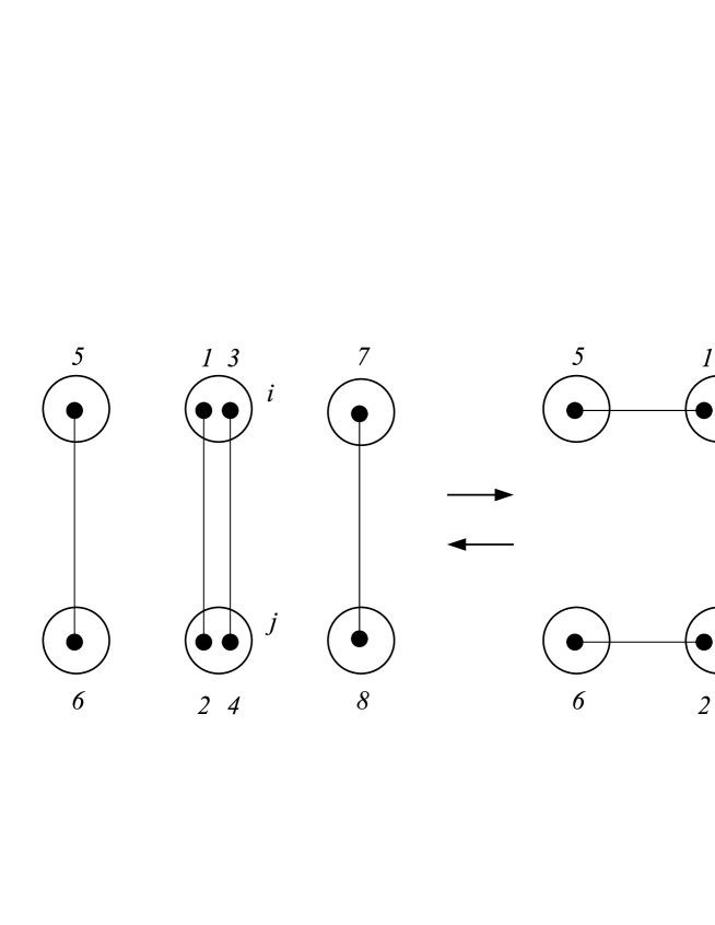
Figure 1: switching for multiple edges

It is easy to see that this switching converts the pairing ${\cal P}\in{\cal C}\big{(}{\bf M}(m)\big{)}$ to a pairing in ${\cal C}\big{(}{\bf M}(0)\big{)}$, provided that none of the following conditions hold (though these are not all entirely necessary):

(i) a pair $x_{g}$ is part of a non-loop multiple edge;

(ii) a pair $x_{g}$ uses a vertex $w$ already adjacent in ${\cal P}$ to $i$ or $j$ by a multiple edge, and $x_{g}$ does not satisfy (i) (this would increase the multiplicity of a multiple edge);

(iii) a pair $x_{g}$ uses a vertex $w$ already adjacent in ${\cal P}$ to $i$ or $j$ by a single edge (this would create a new multiple edge);

(iv) some two pairs $x_{g}$ and $x_{g^{\prime}}$ have a common end-vertex (if this were permitted, two of the new pairs can possibly create a multiple edge).

(v) a pair $x_{g}$ is incident with $i$ or $j$ or is a loop.

We call a switching satisfying these conditions good.

We will bound the probability that a randomly chosen switching is not good, when applied to a random ${\cal P}\in{\cal C}\big{(}{\bf M}(m)\big{)}$. In all cases but (iii) our bound actually applies to an arbitrary ${\cal P}$ rather than a random pairing.

We can choose the pairs one by one. Each of them is potentially any one of the $M_{1}/2$ possible pairs, but it must avoid the $m$ pairs joining $i$ and $j$, as well as up to $m-1$ other pairs already chosen, so there are $M_{1}/2-O(m)$ options. Since $m=o(M_{1})$, the probability that a randomly chosen $x_{g}$ is any given pair, conditional on the previous pairs $x_{1},\ldots,x_{g-1}$, is $O(1/M_{1})$. We will use this observation several times. In particular, for each $1\leq g\leq m$, conditional on the choices of $x_{1},\ldots,x_{g-1}$, the probability that $x_{g}$ is one of $x_{i}$, $i\leq g-1$, or $x_{g}$ is a pair between $i$ and $j$, is $O(m/M_{1})$. Taking the union bound over all $1\leq g\leq m$, the probability that $x_{g}$’s are not distinct, or use a pair between $i$ and $j$, is $O(m^{2}/M_{1})$. By the above observation, this probability is $o(1)$.

Since at most $Z_{i,j}$ pairs are in multiple edges of ${\bf M}(0)$, the probability of (i) occurring is $O(mZ_{i,j}/M_{1})$.

The number of pairs that cause the condition (ii) for any $x_{g}$ is the sum of $d_{w}-2$ over all $w$ such that $iw$ or $jw$ is a multiple edge (excluding $w=i$ or $j$), which is $W_{i,j}+W_{j,i}$. Arguing as for (i), the probability of this occurring is at most $m(W_{i,j}+W_{j,i})/M_{1}$.

For condition (iii), we need to argue about the expected number of switchings in which the condition occurs, when applied to a random pairing ${\cal P}\in{\cal C}\big{(}{\bf M}(m)\big{)}$. To this end, we first estimate the probability $p(i,w)$ that a given point $a$ in vertex $i$ is paired in ${\cal P}$ to a given point $b$ in vertex $w$. This uses the following subsidiary switching argument.

For those pairings ${\cal P}$ containing the pair $ab$, consider switching $ab$ with another randomly chosen pair $a^{\prime}b^{\prime}$ in ${\cal P}$, i.e. delete the pairs $ab$ and $a^{\prime}b^{\prime}$ and insert the pairs $aa^{\prime}$ and $bb^{\prime}$ to create a new pairing ${\cal P}^{\prime}$. Then ${\cal P}^{\prime}$ is also in ${\cal C}\big{(}{\bf M}(m)\big{)}$ provided that neither $a^{\prime}$ nor $b^{\prime}$ is in a vertex adjacent to $i$ or $j$ (there are at most $2\tau$ such points since each corresponds to a unique 2-path starting from $i$ or $j$) and $a^{\prime}b^{\prime}$ is not in a multiple edge (there are at most $2Z$ such points). By assumption (A2) and Lemma 8, the number of ways to choose $a^{\prime}b^{\prime}$ such that ${\cal P}^{\prime}$ is also in ${\cal C}\big{(}{\bf M}(m)\big{)}$ is $\Omega(M_{1})$. Furthermore, each such ${\cal P}^{\prime}$ can be created in at most one way. Hence $p(i,w)=O(1/M_{1})$.

Applying the union bound to all appropriate $(a,b)$ (where we can assume $a$ is not in one of the pairs joining $i$ and $j$), we find that the probability that $iw$ is an edge in ${\cal P}$ is $O\big{(}(d_{i}-2)d_{w}/M_{1})$. Conditional upon this event, the probability that the random pair $x_{g}$ chooses a point in $w$ is $O(d_{w}/M_{1})$. The same considerations as for $i$ apply to $j$, and we conclude that the probability of (iii) occurring for a random ${\cal P}$ is $O(m\sum_{w\leq n}(d_{i}-2+d_{j}-2)d_{w}^{2}/M_{1}^{2})=O\big{(}m(d_{i}+d_{j}-4)(M_{2}+M_{1})/M_{1}^{2}\big{)}$.

Given an arbitrary ${\cal P}$, a randomly chosen switching satisfies (iv) with probability $O(m^{2}M_{2}/M_{1}^{2})$ since there are $O(m^{2})$ choices of $(g,g^{\prime})$, and the number of ways that any two of them can both choose a point in the same vertex is $O(M_{2})$.

Finally, for an arbitrary ${\cal P}$, a randomly chosen switching satisfies (v) with probability $O\big{(}m(d_{i}+d_{j}-4+Z_{0})/M_{1}\big{)}$, since for each $g$, the probability that $x_{g}$ contains a point in $i$ or $j$ is $O((d_{i}+d_{j}-4)/M_{1})$ and the probability it is a loop is $O(Z_{0}/M_{1})$. Here the term $-4$ occurs because there are at least four points in the multiple edge joining $i$ and $j$ that are excluded.

Let $N_{i,j}$ denote the expected number of choices of a good switching, for a uniformly randomly chosen ${\cal P}\in{\cal C}\big{(}{\bf M}(m)\big{)}$, where we distinguish between the $m!$ different ways to assign the labels $1,3,\ldots,2m-1$ to the points in vertex $i$. These induce labels of the points paired with them in $j$. There are two ways to label the ends of each of the chosen pairs, and, using the observation before considering (i), there are $\big{(}1-O(m^{2}/M_{1})\big{)}M_{1}^{m}/2^{m}$ ways to choose the pairs. Hence

$$N_{i,j} = m!M_{1}^{m}\bigg{(}1+O(m)\bigg{(}\frac{Z_{i,j}}{M_{1}}+\frac{W_{i,j}+W_{j,i}}{M_{1}}+\frac{(d_{i}+d_{j}-4)M_{2}}{M_{1}^{2}}+\frac{d_{i}+d_{j}-4+Z_{0}}{M_{1}}\bigg{)}$$ (8)

$$+O(m^{2})\bigg{(}\frac{M_{2}}{M_{1}^{2}}+\frac{1}{M_{1}}\bigg{)}\bigg{)}.$$

On the other hand, speaking informally, the inverse of a good switching will convert a pairing ${\cal P}\in{\cal C}\big{(}{\bf M}(0)\big{)}$ to one in ${\cal C}({\bf M}(m))$. We formally define an inverse switching to be the following operation. Pick $m$ distinct points in vertex $i$ and label them as $2g-1$, $g=1,\ldots,m$; label the point paired with $2g-1$ as $2m+2g-1$; do a similar thing for $j$, producing pairs $\{2g,2m+2g\}$ as in the right hand side of Figure 1; and finally replace the pairs $\{2g-1,2m+2g-1\}$ and $\{2g,2m+2g\}$ by new pairs $\{2g-1,2g\}$ and $\{2m+2g-1,2m+2g\}$ for all appropriate $g$. An inverse switching is called good if it creates a pairing in ${\cal C}\big{(}{\bf M}(m)\big{)}$, i.e. if it has the reverse effect of a good switching applied to a pairing in ${\cal C}\big{(}{\bf M}(m)\big{)}$. Since no pair in ${\cal P}$ joins vertices $i$ and $j$, the inverse switching is good if none of the following conditions holds:

(vi) a pair picked incident with $i$ or $j$ is part of an existing multiple edge or forms a loop;

(vii) a new pair is added in parallel to an existing multiple edge.

(viii) a new pair is added in parallel to an existing single edge.

(ix) a pair picked incident with $i$ has a common end vertex with a pair picked incident with $j$. (Then a new loop would be created.)

We next bound the probability that a randomly chosen inverse switching is not good, when applied to a random ${\cal P}\in{\cal C}\big{(}{\bf M}(0)\big{)}$. Note that there are potentially $[d_{i}]_{m}[d_{j}]_{m}$ inverse switchings, but some of these may not be good.

First consider (vi). The number of pairs incident with vertex $i$ that are already part of a multiple edge is $R_{i,j}$. For those already part of a loop, it is $m_{i,i}$. Thus, the proportion of the initial count of switchings falling into this case is $O(m)\big{(}(R_{i,j}+m_{i,i})/d_{i}+(R_{j,i}+m_{j,j})/d_{j}\big{)}$.

For (vii), again we consider a random pairing. Suppose the points $2g-1$ in vertex $i$ and $2g$ in vertex $j$ are specified, and consider the random pairing ${\cal P}\in{\cal C}\big{(}{\bf M}(0)\big{)}$. Given a multiple edge $uv$, the probability that $2g-1$ and $2g$ are paired with points in $u$ and $v$ respectively is, arguing as for (iii) and switching out the two pairs simultaneously, $O((d_{u}-2)(d_{v}-2)/M_{1}^{2})$. (Here we use $d_{u}-2$ rather than $d_{u}$ since the points paired with $2g-1$ and $2g$ cannot be part of the multiple edge, which has multiplicity at least 2.) Hence, the probability of (vii) is $O(mQ_{i,j}/M_{1}^{2})$.

For (viii), we do not need to consider cases which also fall into (vi). Again we need to consider a random pairing. Suppose the points $2g-1$ in vertex $i$ and $2g$ in vertex $j$ are specified, and consider the random pairing ${\cal P}\in{\cal C}\big{(}{\bf M}(0)\big{)}$. Conditioning on the two pairs containing these points, the rest of ${\cal P}$ is a uniformly random pairing conditional upon all the multiple edges existing as specified by ${\bf M}(0)$. Let $u$ and $v$ be two vertices. The number of ways to choose an ordered pair of points $(a,a^{\prime})$ and $(b,b^{\prime})$ in each of $u$ and $v$ respectively is $[d_{u}]_{2}[d_{v}]_{2}$. Arguing as for (iii), switching three pairs out at once, the probability that $2g-1$ and $2g$ are paired with $a$ and $b$, and $a^{\prime}$ and $b^{\prime}$ form a pair, is $O(1/M_{1}^{3})$. Summing over all $u$ and $v$, we obtain the bound $M_{2}^{2}/M_{1}^{3}$ on the probability that any two chosen points $2g-1$ and $2g$ lead to (viii). By the union bound, the probability that at least one of the $m$ new edges causes condition (viii) is $O(m{M_{2}}^{2}/M_{1}^{3})$.

For (ix), we argue as for (vii), but noting that the probability that $2g-1$ and $2g$ are paired with points in the same vertex $w$ is $O\big{(}d_{w}(d_{w}-1)/M_{1}^{2}\big{)}$. Thus, the bound for (ix) is $O(m{M_{2}}/M_{1}^{2})$.

Letting $N^{\prime}_{i,j}$ denote the expected number of good inverse switchings for a random ${\cal P}\in{\cal C}\big{(}{\bf M}(0)\big{)}$, we get

$$\ N^{\prime}_{i,j}=[d_{i}]_{m}[d_{j}]_{m}\bigg{(}1+O(m)\bigg{(}\frac{R_{i,j}+m_{i,i}}{d_{i}}+\frac{R_{j,i}+m_{j,j}}{d_{j}}+\frac{Q_{i,j}}{M_{1}^{2}}+\frac{{M_{2}}^{2}}{M_{1}^{3}}+\frac{{M_{2}}}{M_{1}^{2}}\bigg{)}\bigg{)}.$$ (9)

3.3 Eliminating multiple edges

Before proceeding, we let $\eta_{i,j}({\bf M},m)$ denote the sum of the error terms in (8) and (9), i.e. $\eta_{i,j}({\bf M},m)=mZ_{i,j}/M_{1}+\cdots+m{M_{2}}/M_{1}^{2}$. The last assumption that we will make on the matrix ${\bf M}$ to which we apply the switching analysis is the following.

1. $\eta_{i,j}({\bf M},m_{i,j})\leq\xi_{1}$ for every $i<j$ such that $m_{i,j}\geq 2$.

Moreover, we apply the switchings only in the case that $m=m_{i,j}$ or $m=1$. As with earlier notation, we use $\eta_{i,j}(m)$ to denote $\eta_{i,j}({\bf M},m)$. For each $m\geq 1$, if we let

$$\rho_{m}=\frac{\big{|}{\cal C}\big{(}{\bf M}(m)\big{)}\big{|}}{\big{|}{\cal C}\big{(}{\bf M}(0)\big{)}\big{|}},$$

we have from (8) and (9)

$$\ \rho_{m}=\frac{[d_{i}]_{m}[d_{j}]_{m}}{m!M_{1}^{m}}\big{(}1+O(\eta_{i,j}(m))\big{)}.$$ (10)

Next, write $C_{m}$ for $\big{|}{\cal C}\big{(}{\bf M}(m)\big{)}\big{|}$ (where $m\geq 0$). Then

$$\frac{\big{|}{\cal C}\big{(}{\bf M}\big{)}\big{|}}{\big{|}{\cal C}\big{(}{\bf M}(\clubsuit)\big{)}\big{|}} = \frac{C_{m_{i,j}}}{C_{0}+C_{1}}=\frac{\rho_{m_{i,j}}}{1+\rho_{1}}$$ (11)

$$= \frac{[d_{i}]_{m_{i,j}}[d_{j}]_{m_{i,j}}}{(1+d_{i}d_{j}/M_{1}){m_{i,j}}!M_{1}^{m_{i,j}}}\big{(}1+O(\eta_{i,j}({m_{i,j}}))\big{)}$$

since

$$1+\rho_{1}=1+d_{i}d_{j}/M_{1}+O(\eta_{i,j}(1)d_{i}d_{j}/M_{1})=(1+d_{i}d_{j}/M_{1})(1+O(\eta_{i,j}(1)d_{i}d_{j}/(M_{1}+d_{i}d_{j})),$$

and it is easy to check that $\eta_{i,j}(1)\leq\eta_{i,j}(m_{i,j})$ since ${m_{i,j}}\geq 2$ and the functions $Z_{i,j}$, $W_{i,j}$ etc.  are functions of ${\bf M}$, independent of $m_{i,j}$.

Recall that $(i,j)$ is fixed. The equation above estimates the effect on $\big{|}{\cal C}\big{(}{\bf M}\big{)}\big{|}$ of changing an $(i,j)$-entry of $\bf M$ (and simultaneously $(j,i)$, to keep ${\bf M}$ symmetric) from a number at least 2, to $\clubsuit$. Next, we can select another non-$\clubsuit$ entry of ${\bf M}$ and change it (and the symmetric entry) to $\clubsuit$ using the same procedure. Let ${\bf M}_{\clubsuit}$ be the matrix with all off-diagonal entries equal to $\clubsuit$ and each $(i,i)$ entry equal to $m_{i,i}$, and let ${\mathcal{H}}({\bf M})=\{(i,j):i<j,m_{i,j}\geq 2\}$. Then, applying (11) for each $(i,j)\in{\mathcal{H}}({\bf M})$, we obtain the formula

$$\ \frac{\big{|}{\cal C}\big{(}{\bf M}\big{)}\big{|}}{\big{|}{\cal C}\big{(}{\bf M}_{\clubsuit}\big{)}\big{|}}=\exp\big{(}O\big{(}\eta({\bf M})\big{)}\big{)}\prod_{(i,j)\in{\mathcal{H}}({\bf M})}\frac{[d_{i}]_{m_{i,j}}[d_{j}]_{m_{i,j}}/(m_{i,j}!M_{1}^{m_{i,j}})}{1+d_{i}d_{j}/M_{1}},$$ (12)

as long as

$$\sum_{(i,j)\in{\mathcal{H}}({\bf M})}\eta_{i,j}(m_{i,j})=O\big{(}\eta({\bf M})\big{)}.$$

Note that since $\sum_{(i,j)\in{\mathcal{H}}({\bf M})}m_{i,j}=Z({\bf M})$, $Z\leq Z_{2}$, and since $d_{i}\geq d_{j}$ as $i<j$, terms in $\sum_{(i,j)\in{\mathcal{H}}({\bf M})}\eta_{i,j}(m_{i,j})$ like $d_{j}/M_{1}$ drop out, and we can take

$$\eta\big{(}{\bf M}\big{)}=\frac{Z_{2}+ZZ_{0}}{M_{1}}+\frac{M_{2}Z_{2}}{M_{1}^{2}}+\frac{M_{2}^{2}Z}{M_{1}^{3}}$$

$$+\sum_{(i,j)\in{\mathcal{H}}({\bf M})}m_{i,j}\Bigg{(}\frac{Z_{i,j}+W_{i,j}+W_{j,i}+d_{i}-2}{M_{1}}+\frac{(d_{i}-2)M_{2}}{M_{1}^{2}}+\frac{R_{i,j}+m_{i,i}}{d_{i}}+\frac{R_{j,i}+m_{j,j}}{d_{j}}+\frac{Q_{i,j}}{M_{1}^{2}}\Bigg{)}.$$ (13)

3.4 Switchings for loops

Recall that given ${\bf M}\in{\cal M}$, ${\bf M}_{\clubsuit}$ is the matrix by changing all off-diagonal entries in ${\bf M}$ to $\clubsuit$. Next, we estimate the ratio $|{\cal C}({\bf M}_{\clubsuit})|/|{\cal C}({{\bf M}_{\rm simple}})|$, where ${{\bf M}_{\rm simple}}$ as defined earlier is the symmetric matrix with $\clubsuit$ in all off-diagonal positions and $0$ on the diagonal.

Fix $1\leq i\leq n$ with $m_{i,i}\geq 1$. Let ${\bf M}(0)$ be the matrix obtained from ${\bf M}_{\clubsuit}$ by changing the $(i,i)$ entry from $m_{i,i}$ to $0$. We use $m$ to denote $m_{i,i}$ for convenience. To eliminate the loops at vertex $i$ in ${\cal C}({\bf M}_{\clubsuit})$, we define the following switching. Take ${\cal P}\in{\cal C}({\bf M}_{\clubsuit})$ and label the $m$ loops at $i$ by $1,\ldots,m$. For the $g$th loop at $i$, label the endpoints $2g-1$ and $2g$ (for $1\leq g\leq m$). Pick $m$ distinct pairs in ${\cal P}$, labelling the endpoints of the $g$th pair $2m+2g-1$ and $2m+2g$, and then pick another $m$ distinct pairs and label the endpoints of the $g$th of this lot of pairs $4m+2g-1$ and $4m+2g$. The switching replaces pairs $\{2g-1,2g\}$, $\{2m+2g-1,2m+2g\}$ and $\{4m+2g-1,4m+2g\}$ by $\{2g-1,2m+2g-1\}$, $\{2g,4m+2g\}$ and $\{2m+2g+4m+2g-1\}$. See Figure 2 for an illustration. Let $v_{j}$ denote the vertex containing point $j$ for all $2m+1\leq j\leq 6m$. We say a switching is good if none of the following conditions holds:

1. $v_{j}=i$ for some $2m+1\leq j\leq 6m$, or the vertices in the set $\{v_{j},\ 2m+1\leq j\leq 6m\}$ are not all distinct;

2. $i$ is already adjacent to some $v_{2m+2g-1}$ or to some $v_{4m+2g}$;

3. $v_{2m+2g}$ is already adjacent to $v_{4m+2g-1}$.

Figure 2: switching for loops

As in the multiple edge case, the inverse switching has the obvious natural definition. Pick $2m$ points in $i$ and label them $1,\ldots,2m$. Let the point paired to $2g-1$ be labelled $2m+2g-1$ and the point paired to $2g$ be labelled $4m+2g$, for all $1\leq g\leq m$. Pick another $m$ distinct pairs and label their endpoints $2m+2g$ and $4m+2g-1$ for $1\leq g\leq m$. The inverse switching replaces $\{2g-1,2m+2g-1\}$, $\{2g,4m+2g\}$ and $\{2m+2g,4m+2g-1\}$ by $\{2g-1,2g\}$, $\{2m+2g-1,2m+2g\}$ and $\{4m+2g-1,4m+2g\}$. Again, let $v_{j}$ denote the vertex containing point $j$ for all $2m+1\leq j\leq 6m$. We say an inverse switching is good if none of the following conditions holds

1. the vertices in $\{v_{j},\ 2m+1\leq j\leq 6m\}$ are not all distinct;

2. $v_{2m+2g-1}$ is adjacent to $v_{2m+2g}$; or $v_{4m+2g-1}$ is adjacent to $v_{4m+2g}$.

We will use the following auxiliary functions of ${\bf M}\in{\cal M}$, some of which have already been defined.

• $Z_{0}({\bf M})=\sum_{u\leq n}m_{u,u}$;

• $Z_{i,i}({\bf M})=Z_{0}({\bf M})-m_{i,i}$;

• $Z_{3}({\bf M})=\sum_{u\leq n}m_{u,u}^{2}$;

• $K({\bf M})=\sum_{u\leq n}(d_{u}-2)m_{u,u}$;

• $D({\bf M})=\sum_{u\leq n}(d_{u}-2)I_{m_{u,u}\geq 1}$.

Let $N_{i}$ be the expected number of good switchings that can be applied to a random ${\cal P}\in{\bf M}_{\clubsuit}$. There are $m!2^{m}$ ways to label the endpoints of the $m$ loops at $i$. Potentially there are $M_{1}^{2m}$ ways to choose the $2m$ pairs, in order, and label their endpoints. Hence, potentially there can be $M_{1}^{2m}m!2^{m}$ switchings applied to ${\cal P}$. As discussed in the multiple edge case, the cases where the chosen $2m$ pairs are not all distinct contribute a relative error of $O(m^{2}/M_{1})$. Next, we estimate the probability that a random switching is not good when it is applied to a random pairing ${\cal P}$.

For (a), for every $2m+1\leq j\leq 6m$, the probability that $v_{j}=i$ is $O((d_{i}-2)/M_{1})$. (Note that the subtraction of $2$ is caused by the fact that there are two points in $i$ forming a cycle.) Taking the union bound over $j$, the probability that $v_{j}=i$ for some $j$ is $O(m(d_{i}-2)/M_{1})$. Next we consider repeated vertices. For every $j=2m+2g-1$, $1\leq g\leq 2m$, the probability that $v_{j}\neq i$ and $\{j,j+1\}$ forms a loop is $O(Z_{i,i}/M_{1})$; hence, the probability that one of the $2m$ pairs forms a loop is $O(mZ_{i,i}/M_{1})$. Also, for any two of the $2m$ pairs, the probability that they are both adjacent to a vertex $w$ is $O([d_{w}]_{2}/M_{1}^{2})$. Taking the union bound over all $w\leq n$ and all choices of two pairs (there are $O(m^{2})$ of them) produces the bound $O(m^{2}\sum_{w\leq n}[d_{w}]_{2}/M_{1}^{2})=O(m^{2}{M}_{2}/M_{1}^{2})$. Hence, the probability that (a) occurs is $O\big{(}(d_{i}-2)/M_{1}+mZ_{i,i}/M_{1}+m^{2}{M}_{2}/M_{1}^{2}\big{)}$.

Let $w$ be a vertex. Similar to the argument in condition (iii) for multiple edges, the probability that $i$ is adjacent to $w$ in a random ${\cal P}$ is $O((d_{i}-2)d_{w}/M_{1})$. (Note that there are at least two points in $i$ that form a loop and and hence unavailable to be paired to a point in $w$.) Conditional on that, then, for any $1\leq g\leq m$, the probability that either of the points $2m+2g-1$ and $4m+2g$ is in $w$, and (a) does not occur, is $O((d_{w}-1)/M_{1})$. Hence, taking the union bound over $w$ and $g$, the probability that (b) occurs without (a) is $O(m\sum_{w\leq n}[d_{w}]_{2}(d_{i}-2)/M_{1}^{2})=O(m{M}_{2}(d_{i}-2)/M_{1}^{2})$.

By trivial modifications of the same argument, the probability that (c) occurs without (a) is $O(m{M}_{2}^{2}/M_{1}^{3})$.

It follows that

$$N_{i}=M_{1}^{2m}m!2^{m}\Big{(}1+O(m^{2}/M_{1}+(d_{i}-2)/M_{1}+mZ_{i,i}/M_{1}+m^{2}{M}_{2}/M_{1}^{2}+m{M}_{2}(d_{i}-2)/M_{1}^{2}+m{M}_{2}^{2}/M_{1}^{3})\Big{)}.$$

Next, we estimate $N^{\prime}_{i}$, the expected number of good inverse switchings applied to a random ${\cal P}\in{\cal C}({\bf M}(0))$. Potentially, there are $[d_{i}]_{2m}$ ways to choose and label the points $2g-1$, $2g$, $2m+2g-1$, $4m+2g$ for all $1\leq g\leq m$, and there are $M_{1}^{m}$ ways to choose and label the other pairs. Thus, potentially, the number of inverse switchings that can be applied to ${\cal P}$ is $[d_{i}]_{2m}M_{1}^{m}$. As before, the proportion of these potential cases where the $m$ randomly chosen pairs $\{2m+2g,4m+2g-1\}$ are not all distinct is $O(m^{2}/M_{1})$. We next estimate the probability that a random switching is not good.

Condition (d) occurs only if some pair $\{2m+2g,4m+2g-1\}$ forms a loop, or two chosen pairs use a common vertex. The probability of the former is $O(mZ_{i,i}/M_{1})$. We next bound the probability of the latter when a random switching is applied to a random ${\cal P}$. There are two subcases. Arguing as before, it is easy to find the probability that two pairs with the common vertex are both of form $\{2m+2g,4m+2g-1\}$ is $O(m^{2}{M}_{2}/M_{1}^{2})$. In the second subcase, one pair uses $i$ and the other pair is of the form $\{2m+2g,4m+2g-1\}$. We can choose all the points $2g-1$ and $2g$ in vertex $i$ in advance. The probability that one particular such point is paired with a point in a given vertex $w\neq i$ is $O(d_{w}/M_{1})$. Conditional upon that, the probability that a given $2m+2g^{\prime}$ or $4m+2g^{\prime}-1$ is in $w$ is $O((d_{w}-1)/M_{1})$. Multiplying these by the number $m^{2}$ of choices for $g$ and $g^{\prime}$, we see that this subcase contributes the same as the first one. Hence, the probability for (d) to occur is $O(mZ_{i,i}/M_{1}+m^{2}{M}_{2}/M_{1}^{2})$.

For (e), the analysis is similar to (d), and we easily get $O(m{M}_{2}^{2}/M_{1}^{3})$.

We conclude that

$$N^{\prime}_{i}=[d_{i}]_{2m}M_{1}^{m}(1+O(m^{2}/M_{1}+mZ_{i,i}/M_{1}+m^{2}{M}_{2}/M_{1}^{2}+m{M}_{2}^{2}/M_{1}^{3})).$$

3.5 Eliminating loops

Define

$$\kappa_{i}({\bf M})=m_{i,i}^{2}/M_{1}+(d_{i}-2)/M_{1}+m_{i,i}Z_{i,i}/M_{1}+m_{i,i}^{2}{M}_{2}/M_{1}^{2}+m_{i,i}{M}_{2}(d_{i}-2)/M_{1}^{2}+m_{i,i}{M}_{2}^{2}/M_{1}^{3}.$$

Then

$$\frac{|{\cal C}({\bf M})|}{|{\cal C}({\bf M}(0))|}=\frac{[d_{i}]_{2m_{i,i}}}{M_{1}^{m_{i,i}}m_{i,i}!2^{m_{i,i}}}(1+O(\kappa_{i}({\bf M}))),$$

provided that

1. $\kappa_{i}({\bf M})\leq\xi_{1}$ for all $i\leq n$ such that $m_{i,i}\geq 1$.

For every ${\bf M}$, we can repeatedly switch away all loops in pairings in ${\cal C}({\bf M}_{\clubsuit})$ and apply the above estimate for each ratio as required, and consequently obtain

$$\frac{|{\cal C}({\bf M}_{\clubsuit})|}{|{\cal C}({{\bf M}_{\rm simple}})|}=\exp(O(\kappa({\bf M})))\prod_{i\leq n}\frac{[d_{i}]_{2m}}{M_{1}^{m}m!2^{m}},$$ (14)

where $m$ denotes $m_{i,i}$ and

$$\kappa({\bf M}) = \sum_{i\leq n}\kappa_{i}({\bf M})I_{m_{i,i}\geq 1}$$ (15)

$$= Z_{3}/M_{1}+D/M_{1}+Z_{3}{M}_{2}/M_{1}^{2}+K{M}_{2}/M_{1}^{2}+Z_{0}{M}_{2}^{2}/M_{1}^{3}+\sum_{i\leq n}m_{i,i}Z_{i,i}/M_{1}.$$

3.6 Combining the switchings to obtain simple pairings

Define $\xi({\bf M})=\eta({\bf M})+\kappa({\bf M})$. Let ${\cal M}(\xi_{1})$ be the set of ${\bf M}\in{\cal M}$ for which $\xi({\bf M})\leq\xi_{1}$. Obviously every ${\bf M}\in{\cal M}(\xi_{1})$ satisfies all assumptions (A1)–(A4) . (By considering the first term in $\eta({\bf M})$, we get $Z_{2}({\bf M})/M_{1}\leq\xi_{1}$, which implies (A1) and also (A2) since $Z({\bf M})\leq Z_{2}({\bf M})$; (A3) and (A4) are implied as $\eta_{i,j}({\bf M},m_{i,j})\leq\eta({\bf M})$ and $\kappa_{i}({\bf M})\leq\kappa({\bf M})$). Thus, combining (12) and (14), for every ${\bf M}\in{\cal M}(\xi_{1})$,

$$\frac{|{\cal C}({\bf M})|}{|{\cal C}({{\bf M}_{\rm simple}})|}=F({\bf M})\exp(O(\xi_{1})),$$

where

$$F({\bf M})=\prod_{(i,j)\in{\mathcal{H}}({\bf M})}\frac{[d_{i}]_{m_{i,j}}[d_{j}]_{m_{i,j}}/(m_{i,j}!M_{1}^{m_{i,j}})}{1+d_{i}d_{j}/M_{1}}\prod_{i\leq n}\frac{[d_{i}]_{2m_{i,i}}}{(2M_{1})^{m_{i,i}}m_{i,i}!}$$ (16)

From (7) and then (12), we have

$$\frac{|\Phi|}{\big{|}{\cal C}\big{(}{{\bf M}_{\rm simple}}\big{)}\big{|}} = \sum_{{\bf M}\in{\cal M}}\frac{|{\cal C}\big{(}{\bf M})|}{\big{|}{\cal C}\big{(}{{\bf M}_{\rm simple}}\big{)}\big{|}}$$

$$= \frac{S_{1}}{\big{|}{\cal C}\big{(}{{\bf M}_{\rm simple}}\big{)}\big{|}}+\sum_{{\bf M}\in{\cal M}(\xi_{1})}F({\bf M})\exp\big{(}O(\xi_{1})\big{)}$$

$$= \frac{S_{1}}{\big{|}{\cal C}\big{(}{{\bf M}_{\rm simple}}\big{)}\big{|}}+\big{(}1+O(\xi_{1})\big{)}S_{2}$$

where

$$S_{1}=\sum_{{\bf M}\in{\cal M}\setminus{\cal M}(\xi_{1})}|{\cal C}\big{(}{\bf M})|,\qquad S_{2}=\sum_{{\bf M}\in{\cal M}(\xi_{1})}F({\bf M}).$$

Hence

$$\ \frac{|\Phi|}{\big{|}{\cal C}\big{(}{{\bf M}_{\rm simple}}\big{)}\big{|}}(1-S_{1}/|\Phi|)=S\big{(}1+O(1-S_{2}/S)+O(\xi_{1})\big{)}$$ (17)

where

$$\ S=\sum_{{\bf M}\in{\cal M}}F({\bf M})=\prod_{1\leq i<j<n}A_{i,j}\prod_{1\leq i\leq n}B_{i}$$ (18)

and

$$\ A_{i,j}=\sum_{m\geq 0}\frac{[d_{i}]_{m}[d_{j}]_{m}/(m!M_{1}^{m})}{1+d_{i}d_{j}/M_{1}},\quad B_{i}=\sum_{m\geq 0}\frac{[d_{i}]_{2m}}{(2M_{1})^{m}m!}.$$ (19)

Note that the terms $1+d_{i}d_{j}/M_{1}$, for $m=0$ and 1 respectively, in the numerator of $A_{i,j}$ appear from the case that $m_{i,j}=\clubsuit$, which essentially contributes a factor 1 to the first product in (16).

We will later find bounds for $S_{1}/|\Phi|$ and $1-S_{2}/S$. First we analyse $\xi\big{(}{\bf M}\big{)}$ in order to find a suitable value for $\xi_{1}$.

3.7 Bounding $S_{1}$

In this section, our aim is to find a good upper bound, $\xi_{2}$, on $S_{1}/|\Phi|$ for some suitably small value of $\xi_{1}$. Our final error term will be $O(\xi_{1}+\xi_{2})$. We may view $\xi({\bf M})$ as the total of the error bounds for the individual switchings that are relevant to pairing ${\cal P}\in\Phi$ given ${\bf M}({\cal P})$. In earlier applications of the switching method to counting graphs with given degrees, the analogue of $\xi_{1}$ was a bounded multiple of the analogue of ${\bf E}\,\xi({\bf M})$ (viewed in this way). For those familiar with the argument, a bounded multiple is clearly optimal. This was relatively straightforward in those applications because the error bound per switching was a simple function of the basic variables being analysed. Roughly speaking, these correspond to $Z$ and $Z_{0}$. Unfortunately, we cannot afford this luxury in our application because our approach is quite different and we deal with the much more complicated $U$ functions. Consequently, we content ourselves with $\xi_{1}$ and $\xi_{2}$ being approximately the square root of ${\bf E}\,\xi({\bf M}({\cal P}))$. That is, our goal is prove that with probability $1-O(\sqrt{\xi})$, $\xi({\bf M}({\cal P}))\leq\sqrt{\xi}$. We start by evaluating the expectation of each term in $\xi({\bf M}({\cal P}))$. Recall the definitions of $U_{i}$ in (5). We further define

$$U_{6} = \sum_{i\neq j\leq n}\min\{[d_{i}]_{3}[d_{j}]_{3}/M_{1}^{2},d_{i}d_{j}\},$$

$$U_{7} = \sum_{i\neq j\leq n}\frac{[d_{i}]_{2}}{M_{1}}\min\{(d_{i}-2)[d_{j}]_{2}/M_{1}^{2},d_{j}/M_{1}\}.$$

Lemma 9.

We have the following, where ${\cal H}={\cal H}({\bf M}({\cal P}))$ is defined above (12) and all functions are of a pairing ${\cal P}$ taken u.a.r. from $\Phi$. Here $m_{i,j}$ refers to the entry of ${\bf M}({\cal P})$.

$${\bf E}Z=O({U}_{2});\quad{\bf E}Z_{2}=O({M}_{2}^{2}/M_{1}^{2});\quad{\bf E}\sum_{\cal H}m_{i,j}Z_{i,j}=O({U}_{2}^{2});$$

$${\bf E}\sum_{\cal H}m_{i,j}(W_{i,j}+W_{j,i})=O({U}_{3});\quad{\bf E}\sum_{\cal H}m_{i,j}(d_{i}-2)=O({U}_{4});$$

$${\bf E}\sum_{\cal H}m_{i,j}(R_{i,j}/d_{i}+R_{j,i}/d_{j})=O({U}_{5});\quad{\bf E}\sum_{\cal H}m_{i,j}Q_{i,j}=O({U}_{2}{U}_{6});$$

$${\bf E}\sum_{\cal H}m_{i,j}(m_{i,i}/d_{i}+m_{j,j}/d_{j})=O(U_{7});\quad{\bf E}ZZ_{0}=O(U_{2}{M_{2}}/M_{1});$$

$${\bf E}Z_{0}=O({M_{2}}/M_{1});\quad{\bf E}Z_{3}=O({M}_{2}/M_{1}+{M}_{4}/M_{1}^{2});$$

$${\bf E}K=O({M}_{3}/M_{1});\quad{\bf E}D=O(U_{1});\quad{\bf E}\sum_{1\leq i\leq n}m_{i,i}Z_{i,i}=O(M_{2}^{2}/M_{1}^{2}).$$

Proof.  An upper bound on ${\bf E}Z({\cal P})$ is obtained as follows. First, note that if $Y_{u.v}$ is the multiplicity of the edge $uv$ in ${\cal P}$,

$${\bf E}(Y_{u,v}I_{Y_{u,v}\geq 2})\leq{\bf E}\big{(}\min\{[Y_{u,v}]_{2},Y_{u,v}\}\big{)}\leq\min\{{\bf E}[Y_{u,v}]_{2},{\bf E}Y_{u,v}\}.$$

The number of locations for two non-loop pairs in parallel is at most $\sum[d_{u}]_{2}[d_{v}]_{2}$, summed over all vertices $u<v$, and similarly $\sum d_{u}d_{v}$ for just one pair. Since all of the $M_{1}$ points are uniformly at random (u.a.r.) paired in ${\cal P}$, for any constant integer $k>0$, the probability of a given set of $k$ pairs occurring in ${\cal P}$ is

$$\frac{\prod_{i=k}^{M_{1}/2-1}(M_{1}-2i-1)}{\prod_{i=0}^{M_{1}/2-1}(M_{1}-2i-1)}=O(M_{1}^{-k}).$$

Hence, recalling the definition of $U_{2}$ from (5), we have

$$\ {\bf E}Z({\cal P})=\sum_{1\leq u<v\leq n}{\bf E}(Y_{u,v}I_{Y_{u,v}\geq 2})=O(U_{2}).$$ (20)

Similarly,

$$\ {\bf E}Z_{2}({\cal P})={\bf E}\sum_{1\leq u<v\leq n}Y_{u,v}^{2}I_{Y_{u,v}\geq 2}\leq 2\sum_{1\leq u<v\leq n}{\bf E}(Y_{u,v}(Y_{u,v}-1))=O(M_{2}^{2}/M_{1}^{2}).$$ (21)

We apply a similar argument to the other terms in the lemma. Firstly,

$${\bf E}\sum_{\cal H}m_{i,j}{Z_{i,j}}=O(U_{2}^{2}).$$

To see this, note that for any pair of vertices $(u,v)$ of concern other than $(i,j)$, the bound $\min\{d_{u}d_{v}/M_{1},d_{u}^{2}d_{v}^{2}/M_{1}^{2}\}$ is still valid for ${\bf E}Y_{u,v}I_{Y_{u,v}\geq 2}$ even when a given value of $m_{i,j}$ is conditioned upon. Hence the expression is bounded above by $({\bf E}Z({\cal P}))^{2}$.

Next, we show

$$\sum_{\cal H}m_{i,j}(W_{i,j}+W_{j,i})=O(U_{3}).$$ (22)

First notice that

$${\bf E}\sum_{\cal H}Y_{i,j}W_{i,j} = {\bf E}\Big{(}\sum_{1\leq i<j\leq n}m_{i,j}W_{i,j}I_{Y_{i,j}\geq 2}\Big{)}$$ (23)

$$= {\bf E}\Big{(}\sum_{1\leq i<j\leq n}Y_{i,j}I_{Y_{i,j}\geq 2}\sum_{w\notin\{i,j\}}(d_{w}-2)I_{Y_{i,w}\geq 2}\Big{)}.$$

Given any value of $Y_{i,j}\geq 2$, the conditional expectation of $\sum_{w\notin\{i,j\}}(d_{w}-2)I_{Y_{i,w}\geq 2}$ is always bounded by $\sum_{w\leq n}(d_{w}-2)O\big{(}\min\{[d_{i}-2]_{2}[d_{w}]_{2}/M_{1}^{2},1\}\big{)}$ using the fact that

$$\ {\bf P}(Y_{i,w}\geq 2\mid Y_{i,j}\geq 2)=O\big{(}\min\{[d_{i}-2]_{2}[d_{w}]_{2}/M_{1}^{2},1\}\big{)}.$$ (24)

Hence, we can separate the product inside the expectation in (23) and bound its expectation asymptotically (within a constant factor) by the product of the two expectations. We have already shown that

$${\bf E}\Big{(}\sum_{1\leq i<j\leq n}Y_{i,j}I_{Y_{i,j}\geq 2}\Big{)}={\bf E}Z=O(U_{2}).$$

Recalling the definition of $U_{3}$ from (5), we have ${\bf E}\sum_{\cal H}Y_{i,j}W_{i,j}=O(U_{3})$. By swapping the labels of $i$ and $j$ and noting that in the definition of $U_{3}$, $i$ and $j$ are not ordered, we also have ${\bf E}\sum_{\cal H}Y_{i,j}W_{j,i}=O(U_{3})$, and hence (22).

It is straightforward to bound the expectations of all the other terms in the lemma in a similar fashion.    

By Lemma 9 and the definition of $\xi({\bf M})=\eta({\bf M})+\kappa({\bf M})$ where $\eta({\bf M})$ and $\kappa({\bf M})$ are given in (13) and (15), we have ${\bf E}\,\xi({\cal P})=O(\xi_{0})$ where

$$\xi_{0} = U_{5}+U_{7}+\frac{U_{2}^{2}+U_{3}+U_{4}+U_{1}}{M_{1}}+\frac{U_{2}M_{2}+U_{4}M_{2}+U_{2}U_{6}}{M_{1}^{2}}+\frac{U_{2}M_{2}^{2}}{M_{1}^{3}}$$

$$+\frac{M_{2}}{M_{1}^{2}}+\frac{M_{4}+M_{3}M_{2}+M_{2}^{2}}{M_{1}^{3}}+\frac{M_{4}M_{2}+M_{2}^{3}}{M_{1}^{4}}.$$

Note that, by elementary considerations,

$$U_{7}=O(M_{3}M_{2}/M_{1}^{3});\quad\frac{U_{4}}{M_{1}}=O(M_{3}M_{2}/M_{1}^{3});\quad\frac{U_{2}M_{2}}{M_{1}^{2}}=O(M_{2}^{3}/M_{1}^{4});$$

$$M_{4}\leq M_{3}M_{2};\quad M_{4}M_{2}\leq M_{2}^{3};\quad M_{2}^{2}/M_{1}^{3}\leq M_{2}/M_{1}^{2}+M_{2}^{3}/M_{1}^{4}.$$

Moreover, by the hypothesis of Theorem 6 that $\xi=o(1)$, we have (taking the first option in the min functions) $U_{2}U_{6}/M_{1}^{2}=O(M_{2}^{2}M_{3}^{2}/M_{1}^{6})=o(M_{2}M_{3}/M_{1}^{3})$. Thus $\xi_{0}=O(\xi)$ and we have ${\bf E}\xi({\cal P})=O(\xi)$.

Now we set $\xi_{1}$ in the previous sections to be $\sqrt{\xi}$, which is $o(1)$. This definition determines the precise set ${\cal M}(\xi_{1})$ which we have been dealing with since Section 3.6, and ensures that $\xi_{1}=o(1)$ as required by (A1–A4).

Recalling the definition of $S_{1}$ above (17), the following comes immediately from Lemma 9 using Markov’s inequality.

Corollary 10.

Assume that the hypothesis of Theorem 6 holds. With probability $1-O\big{(}\sqrt{\xi}\big{)}$, ${\bf M}({\cal P})\in{\cal M}\big{(}\sqrt{\xi}\big{)}$.

It follows from this corollary that

$$\ \frac{S_{1}}{|\Phi|}={\bf P}\big{(}{\bf M}({\cal P})\notin{\cal M}(\sqrt{\xi})\big{)}=O\big{(}\sqrt{\xi}\big{)}.$$ (25)

3.8 Bounding $S-S_{2}$

Next, as might be foreseen from (17), we wish to bound $1-S_{2}/S$. Define a probability space $\Omega^{*}$ by equipping ${\cal M}$ with a new probability function, in which ${\bf P}({\bf M})$ is proportional to the “weight” $F({\bf M})$ defined in (16). Then, noting that the total weight is $S$, we have $1-S_{2}/S={\bf P}\big{(}{\bf M}\notin{\cal M}(\sqrt{\xi})\big{)}={\bf P}(\xi({\bf M})>\sqrt{\xi})$ by definition of ${\cal M}(\sqrt{\xi})$. (Recall that we set $\xi_{1}=\sqrt{\xi}$ in Section 3.7.) Next, observe that $\Omega^{*}$ is a product space with each $m_{i,j}$ chosen independently at random from the distribution of a random variable $X_{i,j}$ defined as follows, where the normalising factors $A_{i,j}$ and $B_{i}$ are given in (19). Let ${\bf P}(X_{i,j}=\clubsuit)=A_{i,j}^{-1}$ for $i<j$, and

$${\bf P}(X_{i,j}=m) = A_{i,j}^{-1}\frac{[d_{i}]_{m}[d_{j}]_{m}/(m!M_{1}^{m})}{1+d_{i}d_{j}/M_{1}}\quad(i<j,\ m\geq 2)$$

$${\bf P}(X_{i,i}=m) = B_{i}^{-1}\frac{[d_{i}]_{2m}}{m!(2M_{1})^{m}}\quad(m\geq 0).$$

Clearly ${\bf P}\big{(}X_{i,j}\neq\clubsuit\big{)}=O\big{(}[d_{i}]_{2}[d_{j}]_{2}/M_{1}^{2}\big{)}$. Let $\lambda_{i,j}=d_{i}d_{j}/M_{1}$. Since ${\bf P}(X_{i,j}=m)/{\bf P}(X_{i,j}=m-1)\leq\lambda_{i,j}/m$ when $m\geq 3$, and this is the corresponding ratio for the Poisson variable ${\bf Po}(\lambda_{i,j})$, it follows that $X_{i,j}$ in $\Omega^{*}$ is stochastically dominated by ${\bf Po}(\lambda_{i,j})$ (recalling that $\clubsuit$ is treated as 0 in numerical functions). Hence ${\bf E}X_{i,j}=O(d_{i}d_{j}/M_{1})$. Similarly, $X_{i,i}$ is stochastically dominated by ${\bf Po}(\mu_{i})$ where $\mu_{i}=[d_{i}]_{2}/2M_{1}$.

We next show that the expected value of $\xi({\bf M})$ in $\Omega^{*}$ is $O(\xi)$. The general idea is to show that for each auxiliary function $f\in\{Z,Z_{2},\ldots,K,D\}$ defined in Sections 3.1 and 3.5, the expected value ${\bf E}f({\bf M})$ for ${\bf M}\in\Omega^{*}$ is close to that in Lemma 9 for ${\bf M}({\cal P})$ where ${\cal P}$ is a random pairing in $\Phi$. We first verify this in detail for $f=Z$ and $f=Z_{2}$.

By definition, ${\bf E}Z\leq\sum_{i<j}{\bf E}X_{i,j}=\sum_{i<j}O(d_{i}d_{j}/M_{1})$. Moreover, since $X_{i,j}$ is never equal to 1, ${\bf E}X_{i,j}\leq{\bf E}[X_{i,j}]_{2}$. Using the domination by Poisson, this is $O([d_{i}]_{2}[d_{j}]_{2}/M_{1}^{2})$. Thus ${\bf E}Z\leq\sum_{i<j}{\bf E}[X_{i,j}]_{2}=\sum_{i<j}O([d_{i}]_{2}[d_{j}]_{2}/M_{1}^{2})$. Similarly, by the definition of $Z_{2}$, we have ${\bf E}Z_{2}\leq{\bf E}Z+\sum_{i<j}{\bf E}[X_{i,j}]_{2}=\sum_{i<j}O([d_{i}]_{2}[d_{j}]_{2}/M_{1}^{2})$. Hence, recalling the definition of $U_{2}$ from (5), we have

$${\bf E}Z({\bf M})=O(U_{2}),\quad{\bf E}Z_{2}({\bf M})=O(M_{2}^{2}/M_{1}^{2}).$$

A similar argument applies to the other terms in $\xi$. For instance, we may bound ${\bf E}\sum m_{i,j}W_{i,j}$ by the summation of $[d_{w}]_{3}[d_{i}]_{2}^{2}[d_{j}]_{2}$ over ordered triples $(w,i,j)$. To obtain the same error term as before, note that $[d_{i}]_{2}^{2}=O([d_{i}]_{4}+d_{i})$, and we may obtain the other terms in the $\min$ functions in $U_{3}$ using arguments analogous to those used for the case of random ${\cal P}$. The remaining details required for showing ${\bf E}\xi({\bf M})=O(\xi)$ are straightforward. In particular, note that $m_{i,j}$ and $Z_{i,j}$ are, by design, independent, which makes it easy to write the expected value of $m_{i,j}Z_{i,j}$. (This is why we use $Z_{i,j}$ rather than $Z$.) It then follows, by Markov’s inequality, that in $\Omega^{*}$, ${\bf P}(\xi({\bf M})>\sqrt{\xi})=O(\xi_{0}/\sqrt{\xi})=O(\sqrt{\xi})$, and thus by the same argument as before, $1-S_{2}/S={\bf P}\big{(}{\bf M}\notin{\cal M}(\sqrt{\xi})\big{)}=O(\sqrt{\xi})$. Combining this with (25) in (17) produces

$$\ \frac{|\Phi|}{\big{|}{\cal C}\big{(}{{\bf M}_{\rm simple}}\big{)}\big{|}}=S\big{(}1+O(\sqrt{\xi})\big{)}.$$ (26)

3.9 Estimating $S$

Here we obtain a much more user-friendly version of the function $S$ from (18). Note that the extra error term $M_{1}^{-1}$ makes no difference if $\Delta\geq 3$ since then $U_{1}>0$ and $\xi\geq 1/M_{1}$. If $\Delta\leq 2$ then we could slightly modify the following lemma to go further, but in this case the enumeration problem is anyway easily solved by other means.

Lemma 11.

Assume $\xi=o(1)$ and let $\lambda_{i,j}=d_{i}d_{j}/M_{1}$. Then

$$S=(1+O(\xi+M_{1}^{-1}))\exp\left(\frac{M_{1}}{2}-\frac{M_{2}}{2M_{1}}+\frac{M_{3}}{3M_{1}^{2}}-\frac{3}{4}-\sum_{1\leq i<j\leq n}\log(1+\lambda_{i,j})\right).$$

Proof.  We start by analysing $A_{i,j}$. Recall that

$$\ A_{i,j}(1+d_{i}d_{j}/M_{1})=\sum_{m\geq 0}\frac{[d_{i}]_{m}[d_{j}]_{m}}{m!M_{1}^{m}}.$$ (27)

Let $\lambda_{i,j}=d_{i}d_{j}/M_{1}$. We only need to consider the terms with $m\leq m_{0}=\max\{\log^{2}M_{1},C\lambda_{i,j}\}$ for some sufficiently large constant $C>0$. This is because elementary arguments, for instance considering ratios of successive terms, easily show that the terms with $m>m_{0}$ contribute a relative proportion $O(M_{1}^{-C^{\prime}})$ of the total summation, where $C^{\prime}\to\infty$ as $C\to\infty$. By Lemma 8, the maximum degree $\Delta$ is $o(M_{1}^{3/5})$.

We will at first obtain two different formulae, depending on the size of $d_{i}d_{j}$. We are able to put the second formula into a form that is valid in both cases for an appropriate choice of the split between cases. First we need some observations about the equation

$$\ [d]_{m}/d^{m}=\sum_{k=0}^{m-1}s(m,m-k)d^{-k}$$ (28)

where $s(m,m-k)$ is a Stirling number of the first kind. By definition, $s(m,m)=1$ and

$$s(m,m-k)=\sum_{1\leq b_{1}<b_{2}<\cdots<b_{k}<m}\prod_{i=1}^{k}(-b_{i})=\sum_{1\leq b_{k}<m}(-b_{k})s\big{(}b_{k},b_{k}-(k-1)\big{)}\quad\ \mbox{for all}\ 1\leq k<m.$$

Hence, by induction on $k$, $s(m,m-k)$ is a polynomial $P_{k}$ in $m$ of degree at most $2k$, defined by

$$P_{k}(m)=\sum_{b=1}^{m-1}-bP_{k-1}(b),\qquad P_{0}=1$$

using the standard formula for $\sum_{b=1}^{m-1}b^{r}$. Note that this is valid even for $k\geq m$, when it evaluates to 0.

The first part of the above equation also gives $|s(m,m-k)|\leq\Big{(}\sum_{i=1}^{m}i\Big{)}^{k}<m^{2k}$. Hence for any $d$ and $m$ with $m^{2}/d\leq 1/2$ say, and for any integer $0<t\leq m$,

$$\sum_{k=t}^{m-1}|s(m,m-k)|d^{-k}=O(m^{2t}/d^{t}).$$ (29)

Case 1: $d_{i}d_{j}\geq M_{1}^{5/6}$.

Our main object is to analyse $[d_{i}]_{m}[d_{j}]_{m}$ in (27), for which we will use (28). Since $d_{j}\leq\Delta=o(M_{1}^{3/5})$, we have $d_{i}=\Omega(M_{1}^{5/6}/d_{j})=\Omega(M_{1}^{7/30})$. Hence, if $m\leq\log^{2}M_{1}$, then $m^{2}/d_{i}=o(1/M_{1}^{1/5})$, and similarly for $d_{j}$. On the other hand, if $\log^{2}M_{1}<m\leq m_{0}$ then $m=O(\lambda_{i,j})$ and hence $m^{2}/d_{i}=O(d_{i}d_{j}^{2}/M_{1}^{2})=O(\Delta^{3}/M_{1}^{2})=O(M_{1}^{-1/5})$. In both cases, we have by (28) and (29) that for fixed $u$

$$\ [d]_{m}/d^{m}=\sum_{r=0}^{u-1}s(m,m-r)d^{-r}+O(m^{2u}/d^{u})=\sum_{r=0}^{u-1}s(m,m-r)d^{-r}+O(M_{1}^{-u/5}).$$ (30)

Similarly, since $s(m,m-k)$ is a polynomial $P_{k}$ in $m$ of degree at most $2k$,

$$\ s(m,m-r)d_{i}^{-r}s(m,m-w)d_{i}^{-w}\leq m^{2r+2w}/(d_{i}^{r}d_{j}^{w})$$ (31)

for every fixed $r$ and $w$. Thus for $c_{1}=5K-1$ ($K$ fixed) we have

$$[d_{i}]_{m}[d_{j}]_{m}=O(M_{1}^{-K})+d_{i}^{m}d_{j}^{m}\sum_{r=0}^{c_{1}}\sum_{w=0}^{c_{1}-r}s(m,m-r)d_{i}^{-r}s(m,m-w)d_{j}^{-w}.$$

Rewriting the polynomials $P_{k}$ in terms of the falling factorials $[m]_{t}$ using Stirling numbers of the Second kind, we have for each $r$ and $w$ with $r+w\leq c_{1}$, that $s(m,m-r)s(m,m-w)=\sum_{t=0}^{2c_{1}}a_{r,w,t}[m]_{t}$ for some absolute constants $a_{r,w,t}$ where $a_{0,0,0}=1$. Hence

$$\ [d_{i}]_{m}[d_{j}]_{m}=O(M_{1}^{-K})+d_{i}^{m}d_{j}^{m}\sum_{r=0}^{c_{1}}\sum_{w=0}^{c_{1}-r}\sum_{t=0}^{2c_{1}}a_{r,w,t}[m]_{t}d_{i}^{-r}d_{j}^{-w}.$$ (32)

We may now rewrite (27), recalling that terms with $m>\max\{\log^{2}n,C\lambda_{i,j}\}$ can be ignored in (27). Noting that the new terms introduced in the following are similarly negligible, we have

$$A_{i,j}(1+\lambda_{i,j}) = \sum_{m\geq 0}\frac{\lambda_{i,j}^{m}}{m!}\bigg{(}O(M_{1}^{-K})+\sum_{r=0}^{c_{1}}\sum_{s=0}^{c_{1}-r}\sum_{t=0}^{2c_{1}}a_{r,w,t}[m]_{t}d_{i}^{-r}d_{j}^{-w}\bigg{)}.$$

Thus, using

$$\ \sum_{m\geq 0}[m]_{t}\lambda_{i,j}^{m}/m!=\lambda_{i,j}^{t}\exp(\lambda_{i,j})=d_{i}^{t}d_{j}^{t}M_{1}^{-t}\exp(\lambda_{i,j})$$ (33)

we get

$$\ A_{i,j}(1+\lambda_{i,j})\exp(-\lambda_{i,j})=O(M_{1}^{-K})+\sum_{r=0}^{c_{1}}\sum_{w=0}^{c_{1}-r}\sum_{t=0}^{2c_{1}}a_{r,w,t}d_{i}^{t-r}d_{j}^{t-w}/M_{1}^{t}$$ (34)

and hence

$$\ \log\big{(}A_{i,j}(1+\lambda_{i,j})\big{)}=\lambda_{i,j}+O(M_{1}^{-K})+\log\sum_{r=0}^{c_{1}}\sum_{w=0}^{c_{1}-r}\sum_{t=0}^{2c_{1}}a_{r,w,t}d_{i}^{t-r}d_{j}^{t-w}/M_{1}^{t}.$$ (35)

Case 2: $d_{i}d_{j}\leq M_{1}^{1-\epsilon}$ for some $0<\epsilon\leq 1/6$.

In this case, $[d_{i}]_{m}[d_{j}]_{m}\leq M_{1}^{m-m\epsilon}$. Hence, in the summation (19) defining $A_{i,j}$, the sum of terms for $m>c_{2}$ for any constant $c_{2}\geq\lceil K/\epsilon\rceil-1$ is $O(1/M_{1}^{K})$ (with $K$ as in Case 1). That is,

$$A_{i,j}(1+\lambda_{i,j})=O(M_{1}^{-K})+\sum_{m=0}^{c_{2}}[d_{i}]_{m}[d_{j}]_{m}/(m!M_{1}^{m}),$$

and thus it is straightforward to verify that

$$\ \log\big{(}A_{i,j}(1+\lambda_{i,j})\big{)}=O(M_{1}^{-K})+\phi_{c_{2}}\left(\log\sum_{m=0}^{c_{2}}[d_{i}]_{m}[d_{j}]_{m}/(m!M_{1}^{m})\right)$$ (36)

where $\phi_{c_{2}}$ truncates the expansion of the logarithm of the summation, deleting any terms containing $M_{1}^{-u}$ for $u>c_{2}$.

We next rewrite (36) into a form that we show is equivalent to (35) when $c_{2}$ is large enough. (This equivalence could alternatively be shown by direct but tedious—especially in the case of (35)—computation for any particular value of $K$.) It is a quite subtle aspect of our argument that the terms truncated by $\phi_{c_{2}}$ must not be included! (They make no difference for Case 2 but would spoil Case 1.) Fix any positive constant $c_{2}$. Recalling that $s(m,m-k)$ is a polynomial $P_{k}(m)$ of degree at most $2k$, we may start with (28) and apply the argument leading to (32) but retaining all the terms in the expansion (30) for $r\leq c_{2}-1$. Recalling that the polynomials $s(m,m-r)$ do their job even for $m\leq r$, and in (36) we only consider $m\leq c_{2}$ (implying the error in (30) in this case becomes zero), we have for $m\leq c_{2}$

$$[d_{i}]_{m}[d_{j}]_{m}=\sum_{t=0}^{2c_{2}-2}(d_{i}d_{j})^{m}Q_{t}(d_{i}^{-1},d_{j}^{-1})[m]_{t}$$

where, with $a_{r,w,t}$ as in (35),

$$Q_{t}(d_{i}^{-1},d_{j}^{-1})=\sum_{r=0}^{c_{2}-1}\sum_{w=0}^{c_{2}-1}a_{r,w,t}d_{i}^{-r}d_{j}^{-w}.$$

Now let us consider, as a formal power series in $z$,

$$\log\sum_{m=0}^{c_{2}}\frac{[d_{i}]_{m}[d_{j}]_{m}}{m!}z^{m} = \log\sum_{m=0}^{c_{2}}\sum_{t=0}^{m}\frac{(d_{i}d_{j})^{m}}{m!}Q_{t}(d_{i}^{-1},d_{j}^{-1})[m]_{t}z^{m}$$

$$= \log\left(\sum_{t=0}^{c_{2}}Q_{t}(d_{i}^{-1},d_{j}^{-1})\sum_{m=t}^{c_{2}}\frac{(d_{i}d_{j})^{m}}{m!}[m]_{t}z^{m}\right)$$

$$= \log\left(\sum_{t=0}^{c_{2}}Q_{t}(d_{i}^{-1},d_{j}^{-1})\Big{(}\exp(zd_{i}d_{j})(zd_{i}d_{j})^{t}+O(z^{c_{2}+1})\Big{)}\right).$$

where, in the first step, we note that $[m]_{t}=0$ if $t>m$, and in the last step, $O()$ is used in the formal power series sense and follows from the formula for $\sum_{m\geq 0}\frac{x^{m}}{m!}[m]_{t}.$ The latter expression is

$$\log\left(\exp(zd_{i}d_{j})\sum_{t=0}^{c_{2}}Q_{t}(d_{i}^{-1},d_{j}^{-1})(zd_{i}d_{j})^{t})\right)+O(z^{c_{2}+1})$$

$$=zd_{i}d_{j}+\log\left(\sum_{t=0}^{c_{2}}Q_{t}(d_{i}^{-1},d_{j}^{-1})(zd_{i}d_{j})^{t})\right)+O(z^{c_{2}+1}).$$

Hence, substituting $M_{1}^{-1}$ for $z$,

$$\ \phi_{c_{2}}\left(\log\sum_{m=0}^{c_{2}}[d_{i}]_{m}[d_{j}]_{m}/(m!M_{1}^{m})\right)=d_{i}d_{j}/M_{1}+\phi_{c_{2}}\left(\log\sum_{t=0}^{c_{2}}Q_{t}(d_{i}^{-1},d_{j}^{-1})(d_{i}d_{j}/M_{1})^{t})\right).$$ (37)

Note that the right hand side has the same terms as (35) from Case 1, but with a different cut-off. We are free to choose $c_{2}\geq 2c_{1}=10K-2$ (provided $c_{2}\geq\lceil K/\epsilon\rceil-1$), in which case every term in (34) appears in the right hand side of (37) inside the logarithm. As we noted using (29) in Case 1, including a bounded number of extra terms in the expansion in Case 1 adds an error of order $O(M_{1}^{-K})$. Since $a_{0,0,0}=1$, such extra terms would contribute $O(M_{1}^{-K})$ in (35). Assuming that $\epsilon=1/6$ and $K\geq 1$, this shows that (36) is also valid in Case 1 for $c_{2}=10K-2$ (though some terms in the formula will be dominated by the error term).

We can approximate the simpler function $B_{i}$ in a similar way. Recall that

$$B_{i}=\sum_{m\geq 0}\frac{[d_{i}]_{2m}}{(2M_{1})^{m}m!}.$$

When $d_{i}>M_{1}^{4/5}$, we may terminate the expansion of $[d_{i}]_{2m}/d_{i}^{2m}$ at $m=c_{3}$ where $c_{3}=5K-1$ by incorporating an $O(M_{1}^{-K})$ error term, and this leads to

$$\log B_{i}=\frac{d_{i}^{2}}{2M_{1}}+O(M_{1}^{-K})+\log\sum_{s=0}^{c_{3}}\sum_{t=0}^{2c_{3}}b_{s,t}d_{i}^{t-s}/M_{1}^{t},$$ (38)

analogous to (35), where $b_{s,t}$ are absolute constants independent of $d_{i}$ with $b_{0,0}=1$. On the other hand, for $d_{i}\leq M_{1}^{4/5}$, we may terminate the summation in $B_{i}$ at $m=c_{4}$ such that $c_{4}\geq 5K-1$ by incorporating an $O(M_{1}^{-K})$ error, and this yields

$$\log B_{i}=O(M_{1}^{-K})+\phi_{c_{4}}\left(\log\sum_{m=0}^{c_{4}}[d_{i}]_{2m}/(m!(2M_{1})^{m})\right).$$ (39)

With the same argument as for $A_{i,j}$, with any choice of fixed $c_{4}\geq 2c_{3}=10K-2$, all significant terms in (38) appear in (39) and all terms in (39) not appearing in (38) are insignificant when $d_{i}>M_{1}^{4/5}$. Thus (39) is valid for any $d_{i}$ satisfying the conditions of the lemma.

We now choose $K=3$ in both (36) and (39) and consequently, to ensure the equivalence shown above, $c_{2}=c_{4}=28$, to obtain from (18)

$$S = \exp\left(\sum_{1\leq i<j\leq n}\log A_{i,j}+\sum_{1\leq i\leq n}\log B_{i}\right)$$

$$= \exp\left(\psi({\bf d})-\sum_{1\leq i<j\leq n}\log(1+\lambda_{i,j})+O(n^{2}M_{1}^{-3})\right),$$

where

$$\psi({\bf d})=\sum_{1\leq i<j\leq n}\phi_{28}\left(\log\sum_{m=0}^{28}[d_{i}]_{m}[d_{j}]_{m}/(m!M_{1}^{m})\right)+\sum_{1\leq i\leq n}\phi_{28}\left(\log\sum_{m=0}^{28}[d_{i}]_{2m}/(m!(2M_{1})^{m})\right).$$

Noting that $M_{1}=\Omega(n)$ by our assumption that $d_{1}\geq 1$, the error term $n^{2}M_{1}^{-3}$ is $O(M_{1}^{-1})$. It only remains to show that

$$\psi({\bf d})=\frac{M_{1}}{2}-\frac{M_{2}}{2M_{1}}+\frac{M_{3}}{3M_{1}^{2}}-\frac{3}{4}+O(\xi+M_{1}^{-1}).$$ (40)

The functions $\phi_{28}$ is simply a truncation of the expansion of the logarithm. The result, using Maple for example, is (40), after neglecting all terms that are dominated by $\xi$ or $M_{1}^{-1}$. This completes the proof of Lemma 11.   

We observe that, somewhat surprisingly, in expanding (36), all terms of the form $d_{i}^{r}d_{j}^{w}/M_{1}^{t}$ with $r+w>t+1$ apparently disappear, and similarly all terms in (39) of the form $d_{i}^{w}/M_{1}^{t}$ with $w>t+1$ disappear. The question of finding a proof of this claim was posed, in the case of (36), in a problem session at a meeting in Oberwolfach and immediately solved independently by each of I. Gessel, G. Schaeffer and R. Stanley. Gessel did the same for (39). Using these facts, one can reduce the amount of computation required, by first showing that the terms with $4\leq m\leq 28$ from (36) and (39) are dominated by $\xi+O(M_{1}^{-1})$. Here, it helps to observe that $\sum_{r<w}d_{i}^{r}d_{j}^{w}\leq(M_{2}^{*})^{(r+w)/2}$ for fixed $r,w\geq 2$.

3.10 Completing the proof

Note that our goal is to prove that

$${\bf P}({\mathcal{G}}^{*}(n,{\bf d})\ \mbox{is simple})=(1+O(\sqrt{\xi}+M_{1}^{-1}))\exp\left(-\frac{M_{1}}{2}+\frac{M_{2}}{2M_{1}}-\frac{M_{3}}{3M_{1}^{2}}+\frac{3}{4}+\sum_{i<j}\Big{(}\log(1+d_{i}d_{j}/M_{1})\Big{)}\right)$$ (41)

and then our theorem follows by (2).

Since ${\bf P}({\mathcal{G}}^{*}(n,{\bf d})\ \mbox{is simple})$ equals $|{\cal C}\big{(}{{\bf M}_{\rm simple}}\big{)}|/|\Phi|$ and by (26), it equals $(1+O(\sqrt{\xi}))S^{-1}$. Thus (41) follows by Lemma 11 (and noting that $\xi=O(\sqrt{\xi})$). This completes the proof of Theorem 6.

4 Bounds on the error

Let $\xi$ be defined as in Theorem 6. Due to the complexity of its definition via the $U_{k}$, we present in this section several simpler bounds on $\xi$, which are tight in many situations. We first prove Lemma 7 presented in Section 2.

Proof of Lemma 7.  We can take the first item in each minimum function in the definition of $U_{k}$. So, $U_{2}\leq M_{2}^{2}/M_{1}^{2}$, $U_{3}\leq M_{2}M_{3}M_{4}/M_{1}^{4}$, $U_{4}\leq M_{2}M_{3}/M_{1}^{2}$, $U_{5}\leq M_{2}^{2}M_{3}/M_{1}^{4}$, $U_{1}\leq M_{3}/M_{1}$. This immediately gives the claimed bound on $\xi$ but with an extra term $M_{2}M_{3}/M_{1}^{3}$. However, this term is dominated by $M_{3}/M_{1}^{2}+M_{2}^{2}M_{3}/M_{1}^{4}$. This completes the proof for part (a).

If we have $\Delta=O(M_{1}^{1/2})$, then $M_{2}M_{3}M_{4}/M_{1}^{5}$ is dominated by $M_{2}^{2}M_{3}/M_{1}^{4}$, since $M_{4}=O(d_{1}^{2}M_{2})=O(M_{1}M_{2})$. This bound on $\xi$ is tight within a constant factor, because for such $\Delta$ the first item in the minimum function in each $U_{k}$ dominates the second.    

The following corollary of Lemma 7 is intended for use when there are not too many vertices with degree less than $3$.

Corollary 12.

Putting $M^{*}_{i}=M_{i}+M_{1}$ for $i=2,3$, we have

1. $\xi=O\big{(}M_{3}^{*}(M_{2}^{*})^{2}/M_{1}^{4}+M_{4}M_{3}M_{2}/M_{1}^{5}\big{)}$.

2. If $\Delta=O(\sqrt{M_{1}})$ then $\xi=O\left(M_{3}^{*}(M_{2}^{*})^{2}/M_{1}^{4}\right)$.

Proof.  It is easy to see that $(M_{2}+M_{3})/M_{1}^{2}$ is bounded by $M_{3}^{*}(M_{2}^{*})^{2}/M_{1}^{4}$. It is also easy to see that $M_{2}\leq M_{3}^{*}$ which eliminates $M_{2}^{3}/M_{1}^{4}$ from the bound in Lemma 7. Using the Cauchy inequality, we have $M_{2}^{2}=O(M_{3}^{*}M_{1})$ which eliminates $M_{2}^{4}/M_{1}^{5}$. Now part (a) immediately follows from Lemma 7(a) and part (b) follows from Lemma 7(b).   

The next result follows immediately.

Corollary 13.

Suppose $\Delta=O(\sqrt{M_{1}})$, $M_{1}=O(M_{2})$ and $M_{1}=O(M_{3})$. Then $\xi=\Theta\left(M_{3}M_{2}^{2}/M_{1}^{4}\right).$

Remark. This bound on $\xi$ is tight within a constant factor, since by Lemma 7(b), we have $\xi=\Omega(M_{3}M_{2}^{2}/M_{1})$, and since $M_{1}=O(M_{2})$ and $M_{1}=O(M_{3})$ imply $M_{2}^{*}=\Theta(M_{2})$ and $M_{3}^{*}=\Theta(M_{3})$.

We now present some results more useful when $\Delta$ is large. Without loss of generality we may assume that $d_{1}\geq\cdots\ \geq d_{n}\geq 1$. First, choose $1\leq h<n$ and define $H_{k}=\sum_{i\leq h}[d_{i}]_{k}$ and $L_{k}=M_{k}-H_{k}$.

Lemma 14.

$$\xi = O\left(\frac{H_{1}}{M_{1}}+\frac{H_{1}^{3}+M_{2}+L_{3}}{M_{1}^{2}}+\frac{H_{1}H_{2}M_{2}+M_{2}M_{3}}{M_{1}^{3}}+\frac{L_{2}M_{2}^{2}+L_{2}M_{2}M_{3}}{M_{1}^{4}}\right)$$

$$+\,O\left(\frac{M_{2}^{3}L_{2}+M_{2}M_{3}L_{4}+L_{2}L_{3}H_{4}}{M_{1}^{5}}\right).$$

Proof.  An upper bound on each $U_{k}$ is obtained by using either of the two arguments of each min function. Each min function is a function of one or two vertex degrees. If these degrees involved are at least as large as $d_{h}$, we use the second argument, and otherwise the first. This gives

$$U_{2}\leq L_{2}M_{2}/M_{1}^{2}+H_{1}^{2}/M_{1},$$

$$U_{3}\leq L_{4}M_{3}M_{2}/M_{1}^{4}+H_{4}L_{3}L_{2}/M_{1}^{4}+H_{3}H_{1}L_{3}/M_{1}^{3}+H_{2}H_{1}L_{2}/M_{1}^{2}+H_{1}^{3}/M_{1},$$

$$U_{4}\leq L_{3}M_{2}/M_{1}^{2}+H_{3}L_{2}/M_{1}^{2}+H_{2}H_{1}/M_{1},$$

$$U_{5}\leq L_{3}M_{2}^{2}/M_{1}^{4}+H_{3}L_{2}^{2}/M_{1}^{4}+H_{2}H_{1}L_{2}/M_{1}^{3}+H_{1}^{3}/M_{1}^{2},$$

$$U_{1}\leq L_{3}/M_{1}+H_{1}.$$

In $\xi$, we may omit terms that are dominated by others via inequalities $H_{k}\leq M_{k}$ and $L_{k}\leq M_{k}$. These are $H_{1}^{4}/M_{1}^{3}\leq H_{1}^{3}/M_{1}^{2}$, and several others involving terms with the same denominators.

The result is

$$\xi = O\left(\frac{H_{1}}{M_{1}}+\frac{H_{1}^{3}+M_{2}+L_{3}}{M_{1}^{2}}+\frac{H_{1}H_{2}M_{2}+M_{2}M_{3}}{M_{1}^{3}}\right)$$

$$+\,O\left(\frac{H_{1}^{2}M_{2}^{2}+M_{2}^{2}L_{3}+H_{1}H_{3}L_{3}+M_{2}^{3}+L_{2}M_{2}H_{3}}{M_{1}^{4}}+\frac{L_{2}M_{2}^{3}+M_{2}M_{3}L_{4}+L_{2}L_{3}H_{4}}{M_{1}^{5}}\right).$$

A few more terms can be eliminated as follows.

First, for convenience we replace $L_{2}M_{2}H_{3}/M_{1}^{4}$ by $L_{2}M_{2}M_{3}/M_{1}^{4}$. This is tight because $L_{2}M_{2}L_{3}/M_{1}^{4}\leq M_{2}^{2}L_{3}/M_{1}^{4}$, and the latter is present as a separate error term.

Considering the summations in $L_{3}/L_{2}$, the ratio of corresponding terms is at most $d_{h}-2$, whilst in $H_{3}/H_{2}$ it is greater. Hence $L_{3}/L_{2}\leq d_{h}-2\leq H_{3}/H_{2}$ and consequently $L_{3}/L_{2}\leq M_{3}/M_{2}$. Thus $M_{2}^{2}L_{3}/M_{1}^{4}\leq L_{2}M_{2}M_{3}/M_{1}^{4}$.

For similar reasons, $H_{1}^{2}M_{2}^{2}/M_{1}^{4}\leq H_{1}H_{2}M_{2}/M_{1}^{3}$.

By definition $H_{1}/M_{2}\leq H_{1}/H_{2}=O(1/d_{h})=O(L_{2}/L_{3})$, and hence $H_{1}H_{3}L_{3}\leq L_{2}M_{2}H_{3}\leq L_{2}M_{2}M_{3}$.

Note that $M_{2}^{3}=O(H_{2}^{3}+L_{2}M_{2}^{2})$. Trivially $H_{2}\leq H_{1}^{2}\leq H_{1}M_{1}$, and thus $H_{2}^{3}/M_{1}^{4}\leq H_{1}H_{2}^{2}/M_{1}^{3}\leq H_{1}H_{2}M_{2}/M_{1}^{3}$, which appears in the bound on $\xi$. So we can replace the term $M_{2}^{3}/M_{1}^{4}$ by $L_{2}M_{2}^{2}/M_{1}^{4}$.

The stated bound on $\xi$ follows.   

Having $\Delta=\Omega(\sqrt{M_{1}})$ will permit further simplifications for an appropriate choice of $h$, as in the following lemma. It is easy to see that, for this value of $h$, these bounds are as tight as that in Lemma 14.

Lemma 15.

Suppose that $d_{h}=\Omega(\sqrt{M_{1}})$ and $d_{h+1}=O(\sqrt{M_{1}})$ for some $1\leq h\leq n-1$. Then

(a) $$\xi=O\left(\frac{H_{1}H_{2}^{2}+M_{2}M_{3}}{M_{1}^{3}}+\frac{L_{2}M_{2}M_{3}}{M_{1}^{4}}+\frac{L_{2}L_{3}H_{4}}{M_{1}^{5}}\right);$$

(b) if moreover $$L_{2}=\Omega(M_{1}) M_{2}M_{3}/M_{1}^{3}$$, then the term in (a) can be omitted.

Proof.  As $d_{h}=\Omega(\sqrt{M_{1}})$, we immediately have $M_{2}=\Omega(M_{1})$ and $M_{3}=\Omega(M_{1})$ and thus $M_{2}=O(M_{3})$. Hence,

$$\frac{M_{2}+L_{3}}{M_{1}^{2}}=O\left(\frac{M_{2}M_{3}}{M_{1}^{3}}\right),\quad\frac{L_{2}M_{2}^{2}}{M_{1}^{4}}=O\left(\frac{L_{2}M_{2}M_{3}}{M_{1}^{4}}\right).$$

Moreover, applying Cauchy’s inequality shows that $M_{2}^{2}=O(M_{1}M_{3})$, so $L_{2}M_{2}^{3}/M_{1}^{5}\leq L_{2}M_{2}M_{3}/M_{1}^{4}$. Hence, the formula in Lemma 14 reduces to

$$\xi=O\left(\frac{H_{1}}{M_{1}}+\frac{H_{1}^{3}}{M_{1}^{2}}+\frac{H_{1}H_{2}M_{2}+M_{2}M_{3}}{M_{1}^{3}}+\frac{L_{2}M_{2}M_{3}}{M_{1}^{4}}+\frac{M_{2}M_{3}L_{4}+L_{2}L_{3}H_{4}}{M_{1}^{5}}\right).$$

Next, $d_{h}=\Omega(\sqrt{M_{1}})$ implies that $H_{1}^{2}\geq d_{h}^{2}=\Omega(M_{1})$ and hence $H_{1}/M_{1}=O(H_{1}^{3}/M_{1}^{2})$ which eliminates the first term. It gives moreover that $H_{1}=O(H_{2}/\sqrt{M_{1}})$, and thus $H_{1}^{3}/M_{1}^{2}=O(H_{1}H_{2}^{2}/M_{1}^{3})=O(H_{1}H_{2}M_{2}/M_{1}^{3})$, eliminating the second term. Similarly, we get $H_{1}H_{2}L_{2}/M_{1}^{3}=O(H_{2}H_{3}L_{2}/M_{1}^{4})\leq L_{2}M_{2}M_{3}/M_{1}^{4}$, and thus in the third term $H_{1}H_{2}M_{2}=H_{1}H_{2}^{2}+H_{1}H_{2}L_{2}$ can be replaced by $H_{1}H_{2}^{2}$. Finally, $d_{h+1}=O(\sqrt{M_{1}})$ implies $L_{4}\leq M_{1}L_{2}$, which eliminates $M_{2}M_{3}L_{4}/M_{1}^{5}$. This gives the bound in part (a). If further we have $L_{2}=\Omega(M_{1})$, then $M_{2}M_{3}/M_{1}^{3}=O(L_{2}M_{2}M_{3}/M_{1}^{4})$ and part (b) follows.    

Remark. It is easy to observe (from the definition of $U_{k}$ in (5)) that Lemma 15 gives an asymptotically tight bound on $\xi$ if $d_{i}d_{j}=O(M_{1})$ whenever either $i$ or $j$ is at least $h+1$.

5 Applications

In this section, we will prove Theorems 1–5 of Section 2.

Power-law density-bounded degree sequences: proof of Theorem 2

Recall the definition of power-law density-bounded degree sequences defined in Section 2. It is easy to see that $\Delta=O(n^{1/\gamma})$ and $M_{1}=\Theta(n)$. Therefore $\Delta=O({M_{1}}^{2/5})$, and so by Corollary 12(b), the function $\xi$ of Theorem 6 is $O(M_{3}^{*}(M_{2}^{*})^{2}/M_{1}^{4})$. It is easy to see that $M_{k}^{*}=O(n^{(k+1)/\gamma}+n)$ for $k\geq 2$. Hence, $\xi=o(1)$ when $\gamma>5/2$ is fixed. Thus by Theorem 6 and noting that $1/M_{1}=O(\sqrt{M_{3}^{*}}M_{2}^{*}/M_{1}^{2})$,

$$g({\bf d})=(1+O(\sqrt{M_{3}^{*}}M_{2}^{*}/M_{1}^{2}))\frac{|\Phi|}{\prod_{i=1}^{n}d_{i}!}\exp\left(-\frac{M_{1}}{2}+\frac{M_{2}}{2M_{1}}+\frac{3}{4}+\sum_{i<j}\log(1+\lambda_{i,j})\right).$$ (42)

Next we estimate $\sum_{i<j}\log(1+\lambda_{i,j})$. Taking the Taylor expansion and noting that $\sum_{i<j}\sum_{k\geq 4}\lambda_{i,j}^{k}=O(M_{4}^{2}/M_{1}^{4})$ (since the ratio of the consecutive two terms $\sum_{i<j}\lambda_{i,j}^{k+1}/\sum_{i<j}\lambda_{i,j}^{k}$ is $O(M_{k+1}^{2}/M_{k}^{2}M_{1})=O(\Delta^{2}/M_{1})=o(1)$), we have

$$\sum_{i<j}\log(1+\lambda_{i,j}) = \sum_{i<j}\Big{(}\lambda_{i,j}-\frac{\lambda_{i,j}^{2}}{2}+\frac{\lambda_{i,j}^{3}}{3}\Big{)}+O(M_{4}^{2}/M_{1}^{4}).$$

This we can evaluate using

$$\sum_{i<j}\lambda_{i,j}^{2}=\sum_{i,j}\frac{1}{2}\frac{d_{i}^{2}d_{j}^{2}}{M_{1}^{2}}-\sum_{i}\frac{1}{2}\frac{d_{i}^{4}}{M_{1}^{2}}=(M_{2}+M_{1})^{2}/2M_{1}^{2}+M_{4}/4M_{1}^{2}+O(M_{3}^{*}/M_{1}^{2})$$

and so on. Noting that the error terms $M_{3}^{*}/M_{1}^{2}+M_{2}M_{3}/M_{1}^{3}$ are $O(M_{3}^{*}(M_{2}^{*})^{2}/M_{1}^{4})$, we obtain

$$\sum_{i<j}\log(1+\lambda_{i,j}) = \frac{M_{1}}{2}-\frac{M_{2}}{M_{1}}-\frac{M_{2}^{2}}{4M_{1}^{2}}-\frac{3}{4}+\frac{M_{3}^{2}}{6M_{1}^{3}}+\frac{M_{4}}{4M_{1}^{2}}-\frac{M_{4}^{2}}{8M_{1}^{4}}-\frac{M_{6}}{6M_{1}^{3}}+O\left(\frac{M_{3}^{*}(M_{2}^{*})^{2}}{M_{1}^{4}}\right).$$

Substituting this into (42) we obtain the first formula claimed for $g({\bf d})$. For the second formula, note that for $\gamma>5/2$ we have $M_{4}/M_{1}^{2}+M_{4}^{2}/M_{1}^{4}=O(n^{5/\gamma-2})$ and $M_{6}/M_{1}^{3}=O(n^{7/\gamma-3})$, whereas $M_{3}^{*}(M_{2}^{*})^{2}/M_{1}^{4}=O(n^{10/\gamma-4})$ if $5/2<\gamma<3$. Hence these terms are all bounded by $O(n^{5/\gamma-2})$ for $5/2<\gamma<3$.    

Power-law distribution-bounded sequences: proof of Theorem 3

Let $Z$ be a random variable with a power-law distribution with parameter $\gamma$, let $p_{i}={\bf P}(Z=i)$ and $p_{\geq i}=P(Z\geq i)$. By the definition of power-law distribution-bounded sequences, the number of vertices with degree at least $i$ is $O(p_{\geq i}n)$. We may assume that $d_{1}\geq d_{2}\geq\cdots\geq d_{n}$. Then, for every $1\leq i\leq n$, the number of vertices with degree at least $d_{i}$ is at least $i$ and so immediately, $i=O(p_{\geq d_{i}}n)=O(nd_{i}^{1-\gamma})$. This gives

$$d_{i}=O((n/i)^{1/(\gamma-1)})\quad\mbox{for}\ 1\leq i\leq n.$$ (43)

It follows that $M_{1}=\Theta(n)$ and $M_{k}=O(n^{k/(\gamma-1)})$ for every fixed integer $k\geq 2$.

Let $\xi$ be defined as in Theorem 6. Now we can bound each $U_{i}$ tightly. By (43), for all $i$ and $j$, if $ij\leq n^{3-\gamma}$ then $d_{i}d_{j}=\Omega(n)$ and if $ij>n^{3-\gamma}$ then $d_{i}d_{j}=O(n)$. This tells how to evaluate the minima in the functions $U_{i}$ in (5). As an example, we present detailed calculation for a tight bound of $U_{4}$ only. To simplify the notation, we use $f\preceq g$ to denote $f=O(g)$.

$$U_{4} \preceq \sum_{i=1}^{n^{3-\gamma}}\sum_{j=1}^{n^{3-\gamma}/i}[d_{i}]_{2}d_{j}/n+\sum_{i=1}^{n^{3-\gamma}}\sum_{j=n^{3-\gamma}/i}^{n}[d_{i}]_{3}[d_{j}]_{2}/n^{2}+\sum_{i=n^{3-\gamma}}^{n}\sum_{j=1}^{n}[d_{i}]_{3}[d_{j}]_{2}/n^{2}$$

$$\preceq \sum_{i=1}^{n^{3-\gamma}}\sum_{j=1}^{n^{3-\gamma}/i}\frac{(n/i)^{2/(\gamma-1)}(n/j)^{1/(\gamma-1)}}{n}+\sum_{i=1}^{n^{3-\gamma}}\sum_{j=n^{3-\gamma}/i}^{n}\frac{(n/i)^{3/(\gamma-1)}(n/j)^{2/(\gamma-1)}}{n^{2}}$$

$$+\frac{M_{2}}{n^{2}}\sum_{i=n^{3-\gamma}}^{n}(n/i)^{3/(\gamma-1)}.$$

From here, it is straightforward to obtain

$$\frac{U_{4}M_{2}}{M_{1}^{2}}=O(n^{\frac{(3-\gamma)(\gamma-2)+8-3\gamma}{\gamma-1}})=O(n^{\frac{2+2\gamma-\gamma^{2}}{\gamma-1}}),$$

which is $o(1)$ when $\gamma>1+\sqrt{3}$. We neglect the calculations of the other terms in $\xi$ as the approach is similar and these terms are dominated by $U_{4}M_{2}/M_{1}^{2}$ when $\gamma>1+\sqrt{3}$. This completes the proof of the theorem.    

Using $M_{1}$ and $M_{2}$ alone: proof of Theorem 1

We can assume $M_{2}\geq 1$ since otherwise $d_{i}=1$ for all $i$ and the theorem is is true with zero error term. Then we have $M_{2}\geq[\Delta]_{2}$ and $\Delta=O(M_{2}^{1/2})$. Choose $h$ to be the minimum integer for which $d_{h+1}\leq\sqrt{M_{1}}$. If $h\geq 1$, we can easily bound $L_{2}$ and $H_{2}$ by $M_{2}$; $M_{3}$ and $H_{3}$ by $O(M_{2}^{3/2})$ (since $H_{3}\leq M_{3}\leq\Delta M_{2}$); $L_{3}$ by $O(\sqrt{M_{1}}M_{2})$ and $L_{4}$ by $O(M_{1}M_{2})$; and $H_{4}$ by $M_{2}^{2}$ (since $H_{4}\leq\Delta^{2}H_{2}=O(M_{2}^{2}))$. Note that $M_{2}\geq H_{2}\geq(d_{h}-1)H_{1}=\Omega(M_{1}^{1/2}H_{1})$ by the choice of $h$, and so $H_{1}=O(M_{2}/M_{1}^{1/2})$. Define $\xi$ as in Theorem 6. Then, by Lemma 15(a) (and by noting that $M_{2}=\Omega(\sqrt{M_{1}})$ as $h\geq 1$), $\xi=O(M_{2}^{4}/M_{1}^{9/2})$. If $h=0$ (i.e. $\Delta\leq\sqrt{M_{1}}$), we can bound $M_{3}$ by $M_{2}^{3/2}$ and then Corollary 12(b) gives $\xi=O((M_{2}^{3/2}+M_{1})(M_{2}^{2}+M_{1}^{2})/M_{1}^{4})=O(M_{2}^{4}/M_{1}^{9/2}+M_{2}^{3/2}/M_{1}^{2}+1/M_{1})$ (as the terms apart from $1/M_{1}$ are dominated by $M_{2}^{4}/M_{1}^{9/2}$ when $M_{2}=\Omega(M_{1})$ and by $M_{2}^{3/2}/M_{1}^{2}$ otherwise). Thus, $\xi=o(1)$ as long as $M_{2}=o(M_{1}^{9/8})$, and Theorem 1 follows (with its redefinition of $\xi$) by Theorem 6.    

Bi-valued sequences: proof of Theorem 4

Now $M_{i}=[\Delta]_{i}\ell+[\delta]_{i}(n-\ell)$ for every integer $i\geq 1$. It is easy to see that $M_{1}=\Theta(\Delta\ell+\delta n)$. Since $\delta\geq 3$, we have $M_{1}=O(M_{2})$ and $M_{1}=O(M_{3})$. Define $\xi$ as in Theorem 6. We first show that $\xi=o(1)$ as long as either (a) or (b) holds.

By the hypotheses in (a), $\Delta=O(\sqrt{M_{1}})$. Applying Corollary 13,

$$\xi=\Theta\left(\frac{(\Delta^{3}\ell+\delta^{3}n)(\Delta^{4}\ell^{2}+\delta^{4}n^{2})}{\Delta^{4}\ell^{4}+\delta^{4}n^{4}}\right)=O\left(\frac{\Delta^{7}\ell^{3}+\Delta^{3}\delta^{4}\ell n^{2}+\delta^{7}n^{3}}{\Delta^{4}\ell^{4}+\delta^{4}n^{4}}\right)=o(1),$$

as it is easy to verify that $\Delta^{4}\delta^{3}\ell^{2}n=O(\Delta^{7}\ell^{3}+\delta^{7}n^{3})$. This proves part (a).

Now we prove part (b). By our assumptions, $\Delta^{5}\ell^{3}=o(\delta^{3}n^{3})$ and $\Delta=\Omega((\delta n)^{1/2})$. We first show that $\Delta\ell<\delta n$. Suppose not, then

$$\frac{\Delta^{5}\ell^{3}}{\delta^{3}n^{3}}\geq\Delta^{2}=\Omega(\delta n),$$

contradicting the assumption that $\Delta^{5}\ell^{3}/\delta^{3}n^{3}=o(1)$. Thus $\Delta\ell<\delta n$ and immediately $M_{1}=\Theta(\delta n)$. So $\Delta=\Omega(\sqrt{\delta n})$ implies that $\Delta=\Omega(\sqrt{M_{1}})$. Applying Lemma 15 with $h=\ell$, we have (using $\delta\leq\Delta\leq n$)

$$\xi = O\left(\frac{\Delta^{5}\ell^{3}}{\delta^{3}n^{3}}+\frac{(\Delta^{3}\ell+\delta^{3}n)\delta^{2}n(\Delta^{2}\ell+\delta^{2}n)}{\delta^{4}n^{4}}+\frac{\Delta^{4}\ell\delta^{5}n^{2}}{\delta^{5}n^{5}}\right)$$

$$= O\left(\frac{\Delta^{5}\ell^{3}}{\delta^{3}n^{3}}+\frac{\Delta^{5}\ell^{2}}{\delta^{2}n^{3}}+\frac{\delta^{3}}{n}+\frac{\Delta^{3}\ell}{n^{2}}\right)=o(1).$$

We have now shown that under any condition of (a,b), $\xi=o(1)$. It is easy to see that both $M_{3}/M_{1}^{2}$ and $1/M_{1}$ are dominated by $\xi$ in each case. So the theorem follows by Theorem 6.   

Remark. We have obtained as strong a result as if we had evaluated the expression for $\xi$ in Theorem 6 directly rather than using the results of Section 4. This follows by the remark after Lemma 15, and by noting that in (b) we can assume $\delta\Delta<M_{1}$ (since $M_{1}=\Theta(\delta n)$ and $\Delta<n$). The results in (a) and (b) are similarly tight.

Long-tailed power-law degree sequences: proof of Theorem 5

Choose $h$ to be the minimum integer for which $d_{h+1}<n^{\alpha}$. If $h=0$, the degrees are uniformly bounded, which is a case treated in [4]. However, the error term there is only $o(1)$. Instead, we are done by [17, Theorem 4.6], where the error term is $O(1/n)$ which is clearly $O(\sqrt{\xi})$, with $\xi$ as defined in the theorem statement. Otherwise, $d_{h}=\Omega(n^{\alpha})=\Omega(\sqrt{M_{1}})$, since $\alpha>1/2$. Moreover, by part (a) of the definition of these degree sequences, any component that is less than $n^{\alpha}$ is bounded. So $d_{h+1}=O(\sqrt{M_{1}})$, and we can apply Lemma 15. It is easy to verify that $\Delta=O(n^{\alpha+\beta/\gamma})$ and, in the notation of Lemmas 15 and 14, $H_{1}=O(n^{\alpha+\beta})$ for $\gamma>2$, $H_{1}=O(n^{\alpha+\beta}\log n)$ for $\gamma=2$, and $H_{1}=O(n^{\alpha+2\beta/\gamma})$ for $1<\gamma<2$. By our assumption on $\beta$, it is easy to verify that $H_{1}=o(n)$ always. For every fixed $k\geq 2$, $H_{k}=O(n^{k\alpha+(k+1)\beta/\gamma})$ since $\gamma<3$, and $L_{k}=O(n)$, and moreover $L_{1}=\Theta(n)$. This implies that $M_{1}=\Theta(n)$. Now define $\xi$ as in Theorem 6. By Lemma 15 and using $\alpha>1/2$, it is easy to check that

$$\xi=\left\{\begin{array}[]{ll}O(n^{5\alpha+\beta+6\beta/\gamma-3})&\mbox{if $2<\gamma<3$}\\ O(n^{5\alpha+\beta+3\beta-3}\log n)&\mbox{if $\gamma=2$}\\ O(n^{5\alpha+8\beta/\gamma-3})&\mbox{if $1<\gamma<2$}.\end{array}\right.$$

By the assumption on $\beta$, we have $\xi=o(1)$. As $\alpha>1/2$ by our assumption, the bound on $\xi$ presented above obviously dominates $1/n$. The theorem now follows by Theorem 6.    

Acknowledgement

We are grateful to Remco van der Hofstad for a communication on power law distribution-bounded sequences.

References

- [1] W. Aiello, F. Chung and L. Lu, Random evolution in massive graphs, 42nd IEEE Symposium on Foundations of Computer Science (2001), 510- 519.
- [2] W. Aiello, F. Chung, and L. Lu, A random graph model for power law graphs, Experiment. Math. 10 (2001), no. 1, 53- 66.
- [3] R. Albert and A. Barabási, Statistical mechanics of complex networks, Rev. Mod. Phys, (2002).
- [4] E.A. Bender and E.R. Canfield, The asymptotic number of labeled graphs with given degree sequences, J. Combinatorial Theory Ser. A 24 (1978), 296–307.
- [5] M. Boguñá, F. Papadopoulos and D. Kriouko, Sustaining the Internet with hyperbolic mapping, Nature communications 1 (62), 2010.
- [6] B. Bollobás, A probabilistic proof of an asymptotic formula for the number of labelled regular graphs, Europ. J. Combinatorics 1 (1980), 311–316.
- [7] B. Bollobás, O. Riordan, J. Spencer and G. Tusnády, The degree sequence of a scale-free random graph process, Random Structures Algorithms 18 (2001), no. 3, 279- 290.
- [8] C. Borgs, J. Chayes, C. Daskalakis and S. Roch, First to market is not everything: an analysis of preferential attachment with fitness STOC’07 – Proceedings of the 39th Annual ACM Symposium on Theory of Computing, (2007), 135- 144.
- [9] C. Cooper and A. Frieze, A general model of web graphs, Random Structures Algorithms 22 (2003), no. 3, 311 -335.
- [10] F. Chung and L. Lu, The volume of the giant component of a random graph with given expected degrees, SIAM J. Discrete Math. 20 (2006), no. 2, 395 -411.
- [11] P. Erdős and A. Rényi, On random graphs. I. Publ. Math. Debrecen 6 1959, 290–297.
- [12] M. Faloutsos, P. Faloutsos and C. Faloutsos, On power-law relationships of the Internet topology, ACM SIGCOMM Computer Communication Review 29 4 (1999), 251 – 262.
- [13] L. Gugelmann, K. Panagiotou and U. Peter, Random hyperbolic graphs: degree sequence and clustering, Proceeding ICALP’12 Proceedings of the 39th international colloquium conference on Automata, Languages, and Programming II, 573–585.
- [14] S. Janson, The probability that a random multigraph is simple, Combin. Probab. Comput. 18, no. 1–2, (2009) 205–225.
- [15] S. Janson, The probability that a random multigraph is simple, II. arXiv:1307.6344
- [16] R. Kleinberg, Geographic routing using hyperbolic space, Proceedings of the 26th IEEE International Conference on Computer Communications, INFOCOM 07 1902 -1909.
- [17] B.D. McKay, Asymptotics for symmetric 0-1 matrices with prescribed row sums, Ars Combinatoria 19A (1985), 15–25.
- [18] B.D. McKay and N.C. Wormald, Asymptotic enumeration by degree sequence of graphs with degrees , Combinatorica 11 (1991), 369–382.
- [19] M. Mitzenmacher, A brief history of generative models for power law and lognormal distributions, Internet Math 1 (2004), no. 2, 226- 251.
- [20] C.H. Papadimitriou and D. Ratajczak, On a conjecture related to geometric routing, Theoretical Computer Science 344 1, (2005), 3- 14.
- [21] F. Papadopoulos, D. Krioukov, M. Boguñá and A. Vahdat, Greedy forwarding in dynamic scale-free networks embedded in hyperbolic metric spaces, Proceedings of the 29th IEEE International Conference on Computer Communications, INFOCOM 10, 2973- 2981.
- [22] N.C. Wormald, Models of random regular graphs, Surveys in Combinatorics, 1999, London Mathematical Society Lecture Note Series 267 (J.D. Lamb and D.A. Preece, eds) Cambridge University Press, Cambridge, pp. 239–298, 1999.