Integrable models for quantum media
excited by laser radiation:
a method, physical interpretation, and examples

Abstract

A method to build various integrable models for description of coherent excitation of multilevel media by laser pulses is suggested. Distribution functions over the energy levels of quantum systems depending on the time and frequency detuning are obtained. The distributions follow from Schrödinger equation exact solutions and give the complete dynamical description of laser-excited quantum multilevel systems. Interpretation based on the Fourier spectra of the probability amplitudes of a quantum system is presented. The spectra are expressed in terms of orthonormal polynomials and their weight functions. Matrix elements of the dipole transitions between levels are equal to coefficients of the recurrence formula for the orthonormal polynomial system. Some examples are presented. The Kravchuk oscillator family as an integrable model is constructed to describe the coherent excitation dynamics of multilevel resonance media. It is based on the use of the Kravchuk orthogonal polynomials. The Kravchuk oscillator excitation dynamics is described by the binomial distribution of energy level populations and the distribution parameter depends on excitation conditions. Two known basic models in quantum physics – the harmonic oscillator and two-level system are the special representatives of the Kravchuk oscillator family.

1 Introduction

In dynamical problems of quantum mechanics there exists a rather small number of integrable models. The harmonic oscillator and two-level system are the most well-known and popular ones for the description of matter-field interaction [1, 2, 3]. The first model is the basic one for all quantum physics but it can not describe the saturation effect that is important in laser physics, resonance nonlinear optics, and coherent population transfer where the second model is used.

In this paper we show that there are many various multilevel quantum systems such that their coherent dynamics in an electromagnetic field can be described exactly in a closed form. A method to construct exact analytical solutions of coherent dynamical equations and some examples are presented. A family of multilevel quantum systems (Kravchuk oscillators) is constructed. The coherent dynamics of the Kravchuk oscillators is described by the binomial distribution of the populations. The family contains both the harmonic oscillator and two-level system as a limiting case and a special one.

The nonstationary problems of coherent excitation of quantum systems have become the subject of great interest in recent years [3]. The coherent excitation process takes place for a short time interval when the relaxation does not destroy the quantum medium coherence induced by radiation. Coherent processes are used for the collisionless multiphoton excitation of molecules in the field of laser radiation, for the laser isotope separation, in studies of coherent effects in resonance media excited by ultrashort pulses, in studies of decoherence channels and searching the ways of decoherence elimination with the goal of using these conditions in quantum technologies and quantum computers, for laser controlled chemical reactions (femtochemistry) and in spectroscopy of selective excitated molecules for studying intramolecular and intermolecular relaxation and characterization of highly exited molecules.

2 Model of a quasi-resonance medium excited by laser radiation

The model is a quantum system with the energy levels $E_{n}=\sum_{k=0}^{n}\hbar{\,}\omega_{k};\quad n=0,1,\ldots,N;$ and the radiative transitions between neighbouring levels. We take into account only the most intensive transitions. Each transition ${n{-}1}\leftrightarrow n$ is characterized by the dipole matrix element $\mu_{n-1,{\,}n}=\mu_{01}f_{n};\quad f_{0}\!=\!0;\quad f_{1}\!\!=\!\!1$. The function $f_{n}$ of dipole transition moments is the basic important characteristic of the multilevel quantum system. It describes the dependence of the matrix elements on energy, i.e. on the number $n$ of an ${n{-}1}\leftrightarrow n$ transition, and $f_{n}$ is normalized to the $0\leftrightarrow 1$ transition.

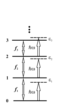
Figure 1: Radiative transitions between adjacent levels; $\omega$ radiation frequency, $\varepsilon_{n}$ frequency detuning, $f_{n}$ dipole moment functions.

It is very seldom that the level energies and transition dipole moments could be calculated from a stationary problem for a quantum system not interacting with radiation and having the hamiltonian ${\rm\bf\hat{H}}_{0}(z)$. As a rule, they are gained from spectral measurements.

A laser pulse switched on at the instant $\tau=0$ has the form $\cal E(\tau)=\cal E_{\ell}\cos{}(\omega_{\ell}\,\tau)$ with the amplitude $\cal E_{\ell}$ and carrier frequency $\omega_{\ell}$; $\tau$ is the time in seconds. The pulse causes the transition of a molecule from initial state $E_{0}=0$ to higher energy levels. The model is depicted in Figure 1. It is a phenomenological model and it extends the well-known two-level one [1, 5]. For the coherent dynamics of multilevel media this model has been used in many papers including [6, 7].

3 Dynamical equations and solution method

In the rotating-wave approximation the coherent dynamics of a quasiresonance quantum system with $N{+}1$ energy levels excited by the monochromatic field is described by the Schrödinger equation written in the dimensionless form [1, 3, 6, 7]:

$$-\mathrm{i}\frac{\mathrm{d}a_{n}(t)}{\mathrm{d}t}= f_{n+1}\exp(-\mathrm{i}\,\varepsilon_{n+1}t)a_{n+1}(t)+f_{n}\exp(+\mathrm{i}\,\varepsilon_{n}t)a_{n-1}(t);$$ (1)

$$n=0,1,\ldots,N;\qquad a_{n}(t\!=\!0)=\delta_{n,0}.$$

Here all the variables and coefficients are dimensionless: $a_{n}(t)$ are the amplitudes of the probability to detect the system at the level $E_{n}$ at the instant $t$, $\varepsilon_{n}$ is the dimensionless frequency detuning on the $n^{th}$ transition $n-1\leftrightarrow n$. Initially the system is located at the zero level.

The field amplitude $\cal E_{\ell}$ is included into the dimensionless time and frequency detuning: $t=\Lambda\tau$, $\varepsilon_{n}=(\omega_{n}-\omega_{\ell})/\Lambda$, where $\Lambda=\mu_{0,1}{\cal E}_{\ell}/2\hbar$ is the Rabi frequency, and $\omega_{n}=(E_{n-1}-E_{n})/\hbar$ is the frequency of the $n^{\mbox{th}}$ transition in the quantum system. The parameter $N$ is any natural number so that the number of the energy levels interacting with radiation is $N{+}1$ along with the number of equations, including $N=\infty$.

Given the known amplitudes $a_{n}(t)$, one can determine the energy level populations $\rho_{n}(t)=\left|a_{n}(t)\right|^{2}\equiv a_{n}(t)a_{n}^{*}(t)$. In other words, it is possible to obtain a distribution function over the energy levels at any instant. The function completely describes the dynamics of a quantum system.

We search the solution of (1) as one of the following expressions

$$a_{n}(t)=\mathrm{e}^{\mathrm{i}{\,}s_{n}{\,}t}b_{n}(t)=\mathrm{e}^{\mathrm{i}{\,}s_{n}{\,}t}\!\int_{A}^{B}\!\!\!\sigma(x)\,p_{0}\;p_{n}(x)\;\mathrm{e}^{\mathrm{i}{\,}r{\,}x{\,}t}\;{\mathrm{d}}x,$$ (2)

$$a_{n}(t)=\mathrm{e}^{\mathrm{i}{\,}s_{n}{\,}t}b_{n}(t)=\mathrm{e}^{\mathrm{i}{\,}s_{n}{\,}t}\sum_{x=0}^{N}\sigma(x)\,p_{0}\;p_{n}(x)\;\mathrm{e}^{\mathrm{i}{\,}r{\,}x{\,}t},$$ (3)

i.e. as the product of a phase factor which does not change the populations $\rho_{n}(t)=a_{n}^{*}(t)\,a_{n}(t)=b_{n}^{*}(t)\,b_{n}(t)$ by the continuous or discrete Fourier transform of $b_{n}(t)$. Here $\omega(x)=rx$ is the continuous or discrete set of Fourier frequencies;

$$S_{n}(x)=\sigma(x)\,p_{0}\;p_{n}(x)$$ (4)

is the Fourier spectrum of the time-dependent function $b_{n}(t)$. The spectrum is expressed in terms of an orthonormal polynomial sequence $\left\{p_{n}(x);\right.$ $\left.n=0,1,\ldots\right\}$ with a continuous or discrete variable $x$; $\sigma(x)$ is the weight function of the polynomials. The orthogonality relation is

$$\int_{A}^{B}\!\!\!\sigma(x)\,p_{m}(x)\,p_{n}(x)\,{\mathrm{d}}x=\delta_{m,\,n}\quad\mbox{or}\quad\sum_{x=0}^{N}\sigma(x)p_{m}(x)p_{n}(x)=\delta_{m,\,n}\,.$$ (5)

Expressions (2), (3) satisfy the initial conditions (1) because of orthogonality (5). It is obvious that the Fourier spectrum (4) of dynamical variables can be discrete (for example when $a_{n}(t)$, $b_{n}(t)$ are time-periodic functions) or continuous. In these different cases one should make a choose between (3) and (2) respectively. By choosing the relevant polynomial sequence one should take into account the number $N+1$ of energy levels and the same number of equations.

Furthermore while making the choice it is very important to take into consideration the known property of any orthonormal polynomials [8, 9]:

$$\bar{f}_{n+1}\,p_{n+1}(x)+\bar{f}_{n}\,p_{n-1}(x)={\rm[}rx+s_{n}{\rm]}\,p_{n}(x);\quad\bar{f}_{1}=1;\quad\bar{f}_{0}=0.$$ (6)

All the coefficients $\bar{f}_{n}$, $r$, $s_{n}$ in the three-term recurrence relation (6) are given for the known orthogonal polynomials, as well as the weight function $\sigma\left(x\right)$. The correct selection appropriate to (1) is the polynomial sequence which satisfies the conditions $\bar{f}_{n}\equiv f_{n}$, i.e. the coefficients $\bar{f}_{n}$ in (6) coincide with the coefficients $f_{n}$ in (1). Then (2) or (3) is the exact solution of (1), as will be shown below.

It should be particularly emphasized that the three-term recurrence relation in form (6) for an orthonormal polynomial sequence is the most important property in solving the problem under investigation. Unfortunately the handbooks do not contain this kind of recurrence formulas, and both orthogonal polynomials and recurrence formulas, as a rule, are written in another standardization. But they can easily be recast to be in form (6).

Substituting, for example, (3) into (1), we arrive at the equations

$$\sum_{x=0}^{N}\sigma(x)p_{0}\,\mathrm{e}^{\mathrm{i}\,r\,x\,t} \left\{f_{n+1}\exp\bigl{(}{-\mathrm{i}(\varepsilon_{n+1}-s_{n+1}+s_{n})t}\bigr{)}\,p_{n+1}(x)+\right.$$

$$\left.\;f_{n}\;\exp\bigl{(}{+\mathrm{i}\left(\varepsilon_{n}-s_{n}+s_{n-1}\right)t}\bigr{)}\,p_{n-1}(x)-[rx+s_{n}]\,p_{n}(x)\right\}=0,$$ (7)

which are equivalent to (1) and govern the coherent dynamics of $N{+}1$-level quantum systems characterized by the parameters $N$, $f_{n}$, $\varepsilon_{n}$. From the set of these systems we will select the systems satisfying the condition $\varepsilon_{n+1}=s_{n+1}-s_{n}$. Then (7) is reduced to be

$$f_{n+1}p_{n+1}(x)+f_{n}p_{n-1}(x)=\left\{rx+s_{n}\right\}p_{n}(x),$$ (8)

and with the constraint $f_{n}\equiv\bar{f}_{n}$ (8) is valid since it coincides with recurrence relation (6) for the orthonormal polynomials. Thus, expression (3) is the exact solution of (1), the coefficients being

$$f_{n+1}=\bar{f}_{n+1},\qquad\varepsilon_{n+1}=s_{n+1}-s_{n}.$$ (9)

A similar reasoning with (2) provides the same result.

Thus, (2) or (3) is the exact solution of (1) with coefficients $f_{n}$, $\varepsilon_{n}$ and the parameter $N$, if the orthonormal polynomial sequence $\{p_{n}(x);\!\!\!\!\quad N\}$ in (2) and (3) contains in its recurrence formula the coefficients $\bar{f}_{n}$, $s_{n}$ (6) satisfying the conditions (9) linking the coefficients of (1) and (6).

It is more natural to construct spectrum (4) with the use of the equation coefficients, i.e. from the characteristics of the quantum system rather then on the basis of polynomial sequence. However, it is more convenient to construct initially the spectrum and then to identify coefficients of (1), amplitudes $a_{n}(t)$, populations $\rho_{n}(t)$, i.e. the quantum system dynamics in the radiation field. We set up the Fourier spectrum in a form of proper known orthonormal polynomials $p_{n}(x)$ where $x$ is a grid and $\sigma(x)$ is a weight function. The proper polynomial sequence should be chosen on the basis of the recurrence relation and $N$. Here we will not consider another method to construct polynomials from a recurrence formula because this problem is difficult to obtain the weight function. At the same time orthogonal polynomial theory is very extensive [10, 11, 12, 13, 14]. There are a lot of various known polynomial sequences and a big field to choose a suitable sequence. It is only necessary to recast the recurrence relations in form (6) for orthonormal polynomial sequences.

In other words, here we solve not a direct problem (to find the solution of (1) for the given quantum system characterized by $N$, $f_{n}$, $\varepsilon_{n}$) but an inverse one: starting from the chosen polynomials, i.e. from the Fourier spectrum of the amplitudes $a_{n}(t)$ we construct a corresponding quantum system, determine the characteristics and build the solution for the dynamical equations (1). At first sight it seems to be a drawback, but the major advantage of such an approach is that it allows one to classify quantum systems, to build the unified solution not only for one system but as well for a set of ones when polynomials contain additional parameters. The theory of orthogonal polynomials (not only classical ones) contains connections between many polynomial sequences. It allows us to transfer these schemes to corresponding quantum systems. A considerable number of the studied polynomials will allow increasing the number of exact solutions describing dynamics of various quantum systems in coherent fields of electromagnetic radiation.

There also exists a deeper connection between the weight function $\sigma(x)$ and corresponding quantum multilevel system because $\sigma(x)$ determines uniquely both the polynomial sequence and the quantum system. It is safe to say that any weight function being the ”progenitor” of polynomial sequence and corresponding quantum system defines the coherent dynamics of a quantum system in the laser radiation field completely within the limits of the assumptions adopted here (rectangular pulse envelope, constant carrier frequency, rotating wave approximation, and transitions between adjacent energy levels).

Theory of orthogonal polynomials is a natural mathematical formalism for the analytical description of the coherent dynamics of various quantum systems excited by laser radiation. All the aforesaid is illustrated using some examples.

4 Harmonic oscillator excited by resonance radiation

This is the first quantum model for the description of one-dimensional movement of a particle with a mass $m$ in the parabolic potential. The Schrödinger equation with the hamiltonian

$${\rm\bf\hat{H}}_{0}(z)=-\frac{\hbar}{2m}\frac{\mathrm{d}^{2}}{\mathrm{d}z^{2}}+\frac{m{\,}\omega^{2}}{2}{\,}z^{2},\qquad-\infty<z<\infty,$$ (10)

where $\omega$ is the oscillator frequency, $z$ is a dimension space coordinate, leads to the boundary-value problem ${\rm\bf\hat{H}}_{0}(z)\varphi(z)=E\varphi(z)$ for eigenvalues and eigenfunctions [1]:

$$E_{n}=\hbar{\,}\omega(n+\textstyle\frac{1}{2});\quad\varphi_{n}(\xi)=\sqrt{\sigma(\xi)}{\,\,}{\rm\hat{H}}_{n}(\xi);\quad n=0,1,\ldots,N=\infty.$$ (11)

Here $\xi=\sqrt{m{\,}\omega/\hbar}{\,\,}z$ is the dimensionless space coordinate, ${\rm\hat{H}}_{n}(\xi)$ are the orthonormal Hermite polynomials

$$\int_{-\infty}^{\infty}\!\!\!\sigma(\xi)\,{\rm\hat{H}}_{n}(\xi)\;{\rm\hat{H}}_{m}(\xi)\;{\rm d}\xi=\delta_{n,\,m},$$ (12)

and $\sigma(\xi)=\exp(-{\xi}^{2})$ is their weight function. In contrast to the real eigenfunctions $\varphi_{n}(\xi)$, the total wave functions of the harmonic oscillator stationary states have the form

$$\psi_{n}(\xi,\tau)=\varphi_{n}(\xi){\,\,}\exp\biggl{(}-{\rm i}{\frac{E_{n}}{\hbar}\tau}\biggr{)}=\sqrt{\sigma(\xi)}{\,\,\,}{\rm\hat{H}}_{n}(\xi){\,\,}\exp\biggl{(}-{\rm i}\omega(n+\textstyle\frac{1}{2})\tau\biggr{)}.$$ (13)

They are orthonormal: $\int_{-\infty}^{\infty}\,\,\psi_{n}^{*}(\xi,\tau)\,\,\psi_{n}(\xi,\tau)\,\,{\rm d}\xi=\delta_{n,\,m}$. This is the case of the harmonic oscillator stationary problem.

The dynamical problem for the oscillator excited by resonance radiation with the frequency $\omega$ is described by (1), where

$$f_{n}=\sqrt{n};\quad\varepsilon_{n}\equiv 0;\quad N=\infty.$$ (14)

The equation has been solved earlier by many various methods [2, 6, 7]. To solve (1) by the method (2), (3), one needs to choose proper orthogonal polynomials. For this purpose, it is necessary to write the recurrence relation (6) for the orthonormal polynomial sequence with $N=\infty$. Resonance excitation of the oscillator is obvious to be non-periodic functions $a_{n}(t)$ with the continuous Fourier spectra, i.e. the proper polynomials are ones of a continuous variable $x$. Among the classical polynomials (Hermite, Laguerre, Jacobi) only the orthonormal Hermite polynomials ${\rm\hat{H}}_{n}(x),\quad n=0,1,\ldots,N=\infty$ satisfy the required recurrence formula

$$\sqrt{n+1}\,{\rm\hat{H}}_{n+1}(x)+\sqrt{n}\,{\rm\hat{H}}_{n-1}(x)=\left[\sqrt{2}\,x+0\,\right]\,{\rm\hat{H}}_{n}(x);\quad n=0,1,\ldots,\infty.$$ (15)

Condition (14) is satisfied. The polynomial weight function is $\sigma(x)=\exp(-x^{2})$, $-\infty{<}x{<}\infty$. Thus the orthonormal Hermite polynomial sequence ${\rm\hat{H}}_{n}(x)$ provides the solution of the dynamical problem.

By substituting ${\rm\hat{H}}_{n}(x)$ into (2) and calculating the integral, one obtains the probability amplitudes

$$a_{n}(t)={\mathrm{i}}^{n}\frac{t^{n}}{\sqrt{n!}}\,\exp\,\left(-t^{2}/2\right),$$ (16)

and then the distribution function $\rho_{n}(t)=a_{n}(t)\,a_{n}^{*}(t)$ (Poisson distribution), i.e. the energy level populations are

$$\rho_{n}(t)=\frac{1}{n!}\,{<\!\!n\!\!>}^{n}\,{\mathrm{e}}^{-<n>};\quad{<\!\!n\!\!>}=t^{2};\quad n=0,1,\ldots,\infty.$$ (17)

The Poisson distribution parameter $<\!\!n\!\!>$ is the average number of quanta absorbed by the oscillator at the instant $t$ because

$$\sum_{n=0}^{\infty}n\rho_{n}=<\!\!n\!\!>,$$ (18)

and the average energy absorbed is

$$<\!E_{n}\!>\,=\hbar\,\omega\sum_{n=0}^{\infty}n\,\rho_{n}=\hbar\,\omega<\!\!n\!\!>.$$ (19)

Although this is the known result, the example, nevertheless, shows clearly that recurrence relation (6) for orthonormal polynomials plays a great role in the choice of a suitable polynomial sequence.

5 Harmonic oscillator excited by non-resonance
radiation

In this case the oscillator dynamics is governed by (1) with $f_{n}$, $N=\infty$ as well but the frequency detunings $\varepsilon_{n}\equiv\varepsilon\neq 0$ are not equal to zero on the transitions. The oscillator is out of resonance; excitation is known to be limited, i.e. $a_{n}(t)$ are periodic functions of time with the discrete Fourier spectra (4), more exactly their spectra are functions of a discrete variable $x$. Therefore the solution of the problem should be sought in form (3) and proper polynomials have to satisfy (6) with

$$\bar{f}_{n}=\sqrt{n},\quad s_{n}=\varepsilon n+\mbox{const},\quad N=\infty.$$ (20)

Among the classical polynomials of a discrete variable, the orthonormal Charlier polynomial sequence [4]

$${\rm\hat{C}}_{n}^{(\mu)}(x);\!\!\!\quad x=0,1,\ldots,\infty;\!\!\!\quad n=0,1,\ldots,\infty;\!\!\!\quad\sigma(x)=\frac{\mu^{x}}{x!}e^{-\mu};\!\!\!\quad\mu>0$$ (21)

satisfies (6) with

$$\bar{f}_{n}=\sqrt{n},\quad r=-1/\!\sqrt{\mu};\quad s_{n}=\mu^{-1/2}\,n+\mu^{1/2}.$$ (22)

Then series (3) with $p_{n}(x)={\rm\hat{C}}_{n}^{(\mu)}(x)$ gives the exact solution of (1) where $f_{n}=\sqrt{n}$; $\varepsilon_{n}\equiv\varepsilon=\mu^{-1/2}$. Owing to the parameter $\mu$, the orthonormal polynomial sequence gives the solution describing excitation by radiation with an arbitrary frequency.

The solution reads

$$a_{n}^{+}=\exp\biggl{(}{\rm i}\left(n\varepsilon+\frac{1}{\varepsilon}\right)t\biggr{)}\,\,\frac{1}{\sqrt{n!}}\,\,\biggl{(}\frac{\theta}{\varepsilon}\biggr{)}^{n}\exp\biggl{(}-\frac{\theta}{\varepsilon^{2}}\biggr{)},\quad\theta=1-\exp({-\rm i}\,\varepsilon\,t),$$ (23)

for $\varepsilon>0$. For $\varepsilon<0$ the solution is $a_{n}^{-}(t)=(-1)^{n}a_{n}^{+}(t)$. The distribution function (energy level populations) has the form

$$\rho_{n}(t)=\frac{1}{n!}\,{<\!\!n\!\!>}^{n}\,{\mathrm{e}}^{-<n>};\quad{<\!\!n\!\!>}=\biggl{(}\frac{2}{\varepsilon}\biggr{)}^{2}\sin^{2}\biggl{(}\frac{\varepsilon}{2}\,\biggr{)};\quad n=0,1,\ldots,\infty.$$ (24)

This is the Poisson distribution as with the preceding example (17). Now the distribution parameter ${<\!n(\varepsilon,t)\!\!>}$ is periodically time-dependent.

In the limit $\varepsilon\to\!0$ (resonance excitation) we obtain $<\!\!n\!\!>_{\mbox{\scriptsize res}}\,=t^{2}$ as in (17). Thus the solution (24) obtained with the use of the Charlier polynomials contains both non-resonance and resonance cases.

The availability of additional parameters in a polynomial sequence is a favorable property since it allows us to obtain the solutions for various conditions of excitation as we have just seen. In this example the parameter $\mu$ is contained in $s_{n}$ of (6). If a parameter is contained in $\bar{f}_{n}$ of the recurrence relation we obtain the solution not only for unique quantum system but for some family of systems as well, as is shown below.

6 Kravchuk polynomials and Kravchuk oscillators

Now we turn to the Kravchuk polynomial sequence ${\rm K}_{\,n}^{\,(p)}(x;N)$; $n=0,1,\dots,N$ of a discrete variable $x=0,1,\dots,N$. The sequence contains two parameters $0<p<1$ and any preassigned positive integer number $N$. The polynomials are orthogonal with respect to the weight function

$$\sigma(x)=\biggl{(}\!{N\atop{x}}\!\biggr{)}p^{\,x}q^{N-x};\quad\!\!\!x=0,1,\ldots,N;\quad\!\!\!\!\biggl{(}\!{N\atop{x}}\!\biggr{)}=\frac{N!}{x!\left(N-x\right)!};\quad\!\!0<p<1;\quad\!\!p+q=1;$$ (25)

In statistical terms it is called the binomial distribution [15]. It was M. Kravchuk who used it for the first time to construct the orthogonal polynomial sequence, these polynomials bear his name [4, 10]. The Kravchuk polynomials generalize the Hermite ones. Using the known recurrence relation for nonnormalized ${\rm K}_{\,n}^{\,(p)}(x;N)$ and their norms $d_{n}$, it is easy to write (6) for the orthonormal Kravchuk polynomials $p_{n}(x)={\rm K}_{\,n}^{\,(p)}(x;N)/d_{n}$. The recurrence relation has coefficients [9]

$$\bar{f}_{n}=\left[n(N\!+\!1\!-\!n)/N\right]^{1/2};\quad r=1/\sqrt{p\,qN};\quad s_{n}=r(p-q)n-rpN.$$ (26)

This means that (3) is the exact solution of (1) with the coefficients

$$f_{n}=\sqrt{\frac{n(N\!+\!1\!-\!n)}{N}};\quad\!\!\varepsilon_{n}=s_{n}-s_{n-1}\equiv\varepsilon=r(p-q)=(p-q)/\sqrt{p\,qN}.$$ (27)

From $f_{n}$ one can see that (3) describes the dynamics of the one-parameter family of $(N{+}1)\mbox{-}$level quantum systems with the dipole moment function $f_{n}$. The family contains various systems including the two-level system (with $N=1$; $f_{1}=1$; $f_{2}=0$) and the harmonic oscillator (in the limit $N\to\infty$; $f_{n}=\sqrt{n}$). Thus, both these fundamental quantum models are the special cases of the Kravchuk oscillators. Since the frequency detuning $\varepsilon_{n}\equiv\varepsilon$ does not depend on the transition number, the energy levels of the Kravchuk oscillator are arranged equidistantly. Each $N$-oscillator is excited by monochromatic radiation with an arbitrary frequency, whereas the detuning $\varepsilon$ is defined by parameters $N$ and $p$ which can be varied. The value $p=1/2$ corresponds to resonant excitation. The dipole moment function $f_{n}$ (for $N<\infty$) increases and then decreases with $n$, the function is symmetric: $f_{n}=f_{N+1-n}$, $n=0,1,\ldots,N$. The Kravchuk oscillator with $N=2$ is the tree-level equidistant equal-Rabi model ($f_{1}=f_{2}=1$, $f_{3}=0$.) For the other $N$ we have various equidistant-level systems with specific energy dependence $f_{n}$ (27) of dipole transitions matrix elements.

7 Coherent dynamics of Kravchuk oscillators family

So the exact solution is defined by the sum (3) with the normalized Kravchuk polynomials $p_{\,n}(x)={\rm\hat{K}}_{\,n}^{\,(p)}(x;N)$. It can be calculated using the representation of the Kravchuk polynomials through hypergeometric function [10]:

$${\rm K}_{\,n}^{\,(p)}(x;N)=(-1)^{n}\biggl{(}\!{N\atop x}\!\biggr{)}p^{\,n}\,\,_{2}F_{1}\left(-n,-x;-N;1/p\right).$$ (28)

The exact solution is thus found to be

$$a_{n}(t)=\left[\biggl{(}\!{N\atop x}\!\biggr{)}(p\,q)^{n}\right]^{1/\,2}\!\!\left(p\,\mathrm{e}^{{\mathrm{i}}\,r\,t}+q\right)^{N-n}\left(\mathrm{e}^{\mathrm{i}\,r\,t}-1\right)^{n}\,\,\exp\{\mathrm{i}\,[(p-q)n-pN\,]\,r\,t\}.$$ (29)

Energy levels populations are expressed as a binomial distribution

$$\rho_{n}(t)=\biggl{(}\!{N\atop n}\!\biggr{)}\,\left[1-y(t)\right]^{N-n}y^{n}(t),\qquad\;y(t)=\frac{1}{N}\left(\frac{2}{r}\right)^{2}\sin^{2}\left(\frac{r}{2}\,t\right),\quad n=0,1,\ldots,N.$$ (30)

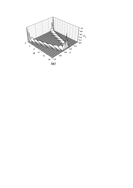
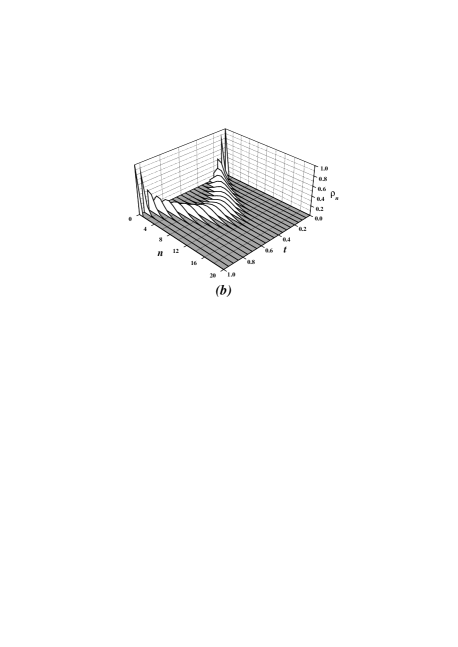
Figure 2: Kravchuk oscillator: excitation dynamics of the system with finite number of levels ($N=20$); figure 2(a) resonant case ($\varepsilon=0$), figure 2(b) nonresonant case ($\varepsilon=0.5$).

The distribution parameter $y(t)$ depends on the proper time $rt$. The solution can be expressed not only through $N$ and $r$ but directly through the parameters of (1) $N$ and $\varepsilon$ as well, because

$$r=1/\sqrt{p\,qN}=\sqrt{\frac{4}{N}+\varepsilon^{2}}\,.$$ (31)

Excitation dynamics of the Kravchuk oscillator with finite number $N+1=21$ of energy levels is shown in Figure 2 both in and beyond resonance. The binomial distribution of the level populations exists at any instant. The movement is periodic: the oscillator stores energy from radiation and then restores it to the field. Outside of resonance only a part of levels are populated during the interaction with radiation.

8 Special cases of the Kravchuk oscillators and their coherent dynamics

In the limit $N\to\infty$, $y(t)\to 0$ so that $\lim_{N\to\infty}Ny(t)=\lambda(t)$, the two-parametric binomial distribution (30) is transformed to the Poisson distribution [15]

$$\rho_{n}(t)=\frac{1}{n!}\,\lambda^{n}(t)\,\mathrm{e}^{-\lambda(t)};\quad\lambda(t)=\left(\frac{2}{\varepsilon}\right)^{2}\sin^{2}\left(\frac{\varepsilon}{2}\,t\right);\quad n=0,1,\ldots,\infty.$$ (32)

Here $\lambda(t)$ is a distribution parameter. In this case $f_{n}=\sqrt{n}$, i.e. we obtain the solution (24) for coherent excitation of the harmonic oscillator by radiation with the frequency detuning $\varepsilon$. In the resonance condition ($\varepsilon=0$), $\lambda(t)=t^{2}$ and the solution takes the form (17).

Another borderline case $N{=}1$ of the solution (30) corresponds to coherent excitation of the two-level model. In this case $f_{1}=1$ (a single transition) and one obtains

$$\rho_{n}(t)=\left(1-y\right)^{1-n}y^{\,n};\quad\;y\equiv y(t)=\frac{1\,}{\Omega^{\,2}}\sin^{2}\left(\Omega\,t\right);\quad\Omega=\sqrt{1+\left(\varepsilon\left/2\right.\right)^{2}};\quad n=0,1.$$ (33)

It coincides with the known solution [1]. The levels populations are $\rho_{0}(t)=1-y,\quad\rho_{1}(t)=y$. At resonance excitation $\Omega=1$, $y=\sin^{2}t$, levels populations are $\rho_{0}=\cos^{2}t$, $\rho_{1}=\sin^{2}t$.

9 Conclusions

Starting from the phenomenological model of a quasiresonance medium excited by coherent radiation, a method is proposed to construct exact analytical solutions of the equations for the probability amplitudes. The method uses continuous or discrete Fourier transforms of the amplitudes, where Fourier spectra are expressed in terms of some orthonormal polynomial sequence multiplied by its weight function. Some exact solutions are obtained and the distribution functions over the quantum system energy levels depending on time and on frequency detuning are presented. The distributions follow from Schrödinger equation exact solutions and give the complete dynamical description of laser-excited quantum multilevel systems when any relaxation processes are eliminated.

The Kravchuk oscillator family as an integrable model has been constructed to describe coherent excitation dynamics of multilevel resonance media. The model is based on the use of the Kravchuk orthogonal polynomials. Kravchuk oscillator excitation dynamics is described with the binomial distribution of energy level populations and a distribution parameter depends on excitation conditions. Two basic models known in quantum physics – the harmonic oscillator and the two-level system are special representatives of the Kravchuk oscillator family.

Physical interpretation of the method is expounded. The Fourier spectra of the amplitudes are expressed in terms of otrhonormal polynomials of a continuous or discrete variable which has meaning of a dimensionless frequency. There is the one-to-one correspondence between the mathematical structures (orthonormal polynomials, their weight function with its range of definition) used and quantum system characteristics (energy levels, dipole moment matrix elements, transitions frequency detunings) along with the dynamical equation coefficients. The recurrence relation for orthonormal polynomials is shown to play the keynote role in the selection of a suitable polynomial sequence to construct the exact solutions for the coherent dynamics of various quantum systems.

In this problem a weight function is shown to be conceptually the only generative object because it defines an orthogonal polynomial sequence, the recurrence formula, quantum system characteristics, dynamical equation coefficients, Fourier spectra of the probability amplitudes, the probability amplitudes proper, energy level populations, and coherent dynamics of the relevant quantum system in the end. If the weight function and its polynomial sequence, respectively, contain some parameters, the solution describes the dynamics of the quantum systems family excited under various conditions.

Orthogonal polynomials are known to be used in stationary quantum problems as well to obtain eigenvalues and eigenfunctions of quantum oscillators [1], including some polynomials of a discrete variable [16]. In the latter case physical interpretation of the results is adaptable to discrete physical space, to discrete quantum mechanics [17]. As it is shown above, in the traditional orthodox quantum mechanics the arguments of orthogonal polynomials differ in physical nature for stationary and dynamical problems: in the former case the argument is a dimensionless space coordinate but in the latter case the argument of the polynomials is the Fourier-frequency of time-dependent functions, i.e. of the probability amplitudes of a quantum system. In a steady-state problem the polynomials are defined in a domain of physical space but in the non-stationary one they are defined in the Fourier space that can be both continuous and discrete. The last case is implemented when the probability amplitudes are periodic functions of time. This case is achieved if radiation interacts with a finite number of energy levels, that is radiation induces a finite number of transitions in a quantum system. Such is indeed the case of practical interest. Therefore orthogonal polynomials of a discrete variable are the most useful tool to solve the problems on coherent excitation of multilevel systems in the common quantum mechanics.

There are a lot of various orthogonal polynomial sequences which can be used to construct exact solutions for dynamics of diverse quantum multilevel models of the laser excited quasiresonance media.

References

- [1] Landau L. D. and Lifshitz E. M. 1977 Quantum mechanics – Non-relativistic Theory (Pergamon Press)
- [2] Baz’ A. I., Zel’dovich Ya. B. and Perelomov A. M. 1966 Scattering, reactions and decay in nonrelativistic quantum mechanics (Israel Program for Scientific Translation in Jerusalem)
- [3] Shore B. W. 1990 The Theory of Coherent Atomic Excitation (Wiley-Interscience)
- [4] Nikiforov A. F., Suslov S. K. and Uvarov V. B. 1991 Classical orthogonal polynomials of discrete variable (Berlin-Heidelberg-New York: Springer-Verlag)
- [5] Allen L., Eberly J. H. 1987 Optical resonance and two-level atoms (Dover, New York)
- [6] Eberly J. H., Shore B. W., Białynicka-Birula Z. and Białynicki-Birula I. 1977 Coherent dynamics of -level atoms and molecules. I. Numerical experiments. Phys. Rev. A. 16 2038
- [7] Makarov A. A. 1977 Coherent excitation of equidistant multilevel systems in a resonant monochromatic field. Sov. Phys.–JETP 45(5) 918
- [8] Suetin P. K. 1976 Classical orthogonal polynomials (Moscow: Science) (In Russian)
- [9] Savva V. A. and Zelenkov V. I. 1992 Multilevel system dynamics and orthogonal polynomials of a discrete variable Preprint No 666 (Minsk: Institute of Physics, Belarus Academy of Sciences) (In Russian)
- [10] Erde lyi A., Magnus W., Oberhettinger F. and Tricomi F. G. 1953 Higher Transcendental Functions, Volume II (Bateman Manuscript Project, McGraw-Hill)
- [11] Chihara T. S. 1978 An Introduction to orthogonal polynomials (Gordon and Breach, New York)
- [12] Ismail M. E. H. 2005 Classical and quantum orthogonal polynomials in one variable (Encyclopedia of mathematics and its applications, Cambridge)
- [13] Gasper G. and Rahman M. 1990 Basic hypergeometric series (Cambridge University Press)
- [14] Koekoek R. and Swarttouw R. F. 1996 The Askey-scheme of hypergeometric orthogonal polynomials and its -analogue Preprint (arXiv:math.CA/9602214)
- [15] Johnson N. L., Kotz S. and Kemp A. W. 1993 Univariate Discrete distributions (Wiley)
- [16] Atakishiev N. M. and Suslov S. K. 1990 Difference analogs of the harmonic oscillator. Theoretical and Mathematical Physics 85(1) 1955
- [17] Odake S. and Sasaki R. 2009 Infinitely many shape invariant discrete quantum mechanical system and new exceptional orthogonal polynomials related to the Wilson and Askey-Wilson polynomials. Phys. Lett. B. 682 130