Random walks and effective optical depth in relativistic flow

Abstract

We investigate the random walk process in relativistic flow. In the relativistic flow, photon propagation is concentrated in the directions of the flow velocity due to relativistic beaming effect. We show that, in the pure scattering case, the number of scatterings is proportional to the size parameter $\xi\equiv L/l_{0}$ if the flow velocity $\beta\equiv v/c$ satisfies $\beta/\Gamma\gg\xi^{-1}$, while it is proportional to $\xi^{2}$ if $\beta/\Gamma\ll\xi^{-1}$ where $L$ and $l_{0}$ are the size of the system in the observer frame and the mean free path in the comoving frame, respectively. We also examine the photon propagation in the scattering and absorptive medium. We find that, if the optical depth for absorption $\tau_{\rm a}$ is considerably smaller than the optical depth for scattering $\tau_{\rm s}$ ($\tau_{\rm a}/\tau_{\rm s}\ll 1$) and the flow velocity satisfies $\beta\gg\sqrt{2\tau_{\rm a}/\tau_{\rm s}}$, the effective optical depth is approximated by $\tau_{*}\simeq\tau_{\rm a}(1+\beta)/\beta$. Furthermore, we perform Monte Carlo simulations of radiative transfer and compare the results with the analytic expression for the number of scattering. The analytic expression is consistent with the results of the numerical simulations. The expression derived in this Letter can be used to estimate the photon production site in relativistic phenomena, e.g., gamma-ray burst and active galactic nuclei.

1. Introduction

Relativistic flows or jets are important phenomena in many astrophysical objects, such as gamma-ray bursts (GRBs) and active galactic nuclei (AGNs). It is widely accepted that most of high-energy emission from these objects arises from the relativistic jets. However, their radiation mechanism is not fully understood. In particular, recent observations of GRBs have indicated the existence of thermal radiation in the spectrum of the prompt emission, which casts a question to standard emission models invoking synchrotron emission.

For example, Ryde et al. (2010) argued that the spectrum of GRB 090902B can be well fitted by a quasi-blackbody with a characteristic temperature of $\sim 290~{}{\rm keV}$. Moreover, it has been reported that some bursts exhibit a thermal component on a usual non-thermal component (e.g., Guiriec et al., 2011; Axelsson et al., 2012). Therefore, investigation of the thermal radiation from GRB jets is crucial to understand the radiation mechanism of GRBs.

The thermal radiation from GRB jets have also been theoretically studied by several methods as follows: fully analytical studies (e.g., Mészáros & Rees, 2000; Rees & Mészáros, 2005), calculations of photospheric emission which treat the thermal radiation as the superposition of blackbody radiation from photosphere (Lazzati et al., 2009, 2011; Mizuta et al., 2011; Nagakura et al., 2011), and detailed radiative transfer calculations with spherical outflows or approximate structures of the jets (e.g., Giannios, 2006, 2012; Pe’er, 2008; Beloborodov, 2010; Pe’er & Ryde, 2011; Lundman et al., 2013; Bégué et al., 2013; Ito et al., 2013).

To study the thermal radiation, treatment of the photosphere needs careful consideration. Lazzati et al. (2009, 2011); Mizuta et al. (2011); Nagakura et al. (2011) performed the hydrodynamical simulations of relativistic jet and calculated the thermal radiation assuming that the photons are emitted at the photosphere which is defined by the optical depth for electron scattering $\tau_{\rm s}=1$. However, the observed photons should be produced in more inner regions with $\tau_{\rm s}\gg 1$ (e.g., Beloborodov, 2013) since the radiation and absorption processes are very inefficient near the photosphere due to the low plasma density. The produced photons propagate through the jet and cocoon which have complicated structure. Thus, radiative transfer calculation of the propagating photons properly evaluating the photon production site is necessary to investigate the thermal radiation from GRB jets.

The photon production site can be estimated by the effective optical depth $\tau_{*}$ (e.g., Rybicki & Lightman, 1979). However, the expression derived in Rybicki & Lightman (1979) is based on an assumption that each scatterings is isotropic in observer frame. The assumption does not strictly hold in any moving media because the photon propagation is concentrated to the direction of the flow due to the beaming effect in the observer frame (Figure 1).

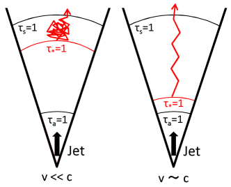
Figure 1.— Schematic pictures of photon propagation in the jet with the velocity $v\ll c$ (left) and $v\sim c$ (right). When $v\ll c$, the scatterings of the photons are approximately isotropic in the observer frame and the surface of $\tau_{*}=1$ is located far from the surface of $\tau_{\rm a}=1$, where $\tau_{\rm a}$ is an optical depth in the absence of the scatterings. When $v\sim c$, the photons are concentrate to the direction of the flow. Thus, the surface of $\tau_{*}=1$ is located close to the surface of $\tau_{\rm a}=1$.

In this letter, we construct an expression for the effective optical depth considering the random walk process in the relativistic flow. In Section 2, we analytically investigate the random walk process in relativistic flow and present the expression for the effective optical depth. In Section 3, we demonstrate that the number of scatterings obtained by the analytic expression agrees with that derived by Monte Carlo simulations. Finally, summary and discussions are presented in Section 4.

2. Analytic expression of random walks in relativistic flow

In this section, we extend the argument for the random walk process shown in Rybicki & Lightman (1979) to the relativistic flow. For simplicity, we assume that the scatterings are isotropic and elastic in the electron rest frame.

2.1. Pure scattering

We first consider purely scattering medium with uniform opacity in which photons are scattered $N$ times. The path of the photons between $i$-1th and $i$th scattering is denoted by ${\bf r}_{i}$. The net displacement of the photon after $N$ scatterings is ${\bf R}={\bf r}_{1}+{\bf r}_{2}+\cdots+{\bf r}_{N}.$ In order to derive the average net displacement of photons $l_{*}$, we first take the square of ${\bf R}$ and then average it,

$$l_{*}^{2}\equiv\langle{\bf R}^{2}\rangle=\sum^{N}_{i=1}\langle{\bf r}^{2}_{i}\rangle+\sum^{N}_{\begin{subarray}{c}i,j\\ i\neq j\end{subarray}}\langle{\bf r}_{i}\cdot{\bf r}_{j}\rangle,$$ (1)

where the angle bracket indicates the average for all photons.

If the medium is at rest relative to an observer, the second term in right hand side of equation (1) vanishes due to the front-back symmetry of the scatterings and only the first term contributes to $l_{*}$. In this case, the first term is calculated as $N\langle\overline{{\bf r}^{2}}\rangle$ where $\overline{{\bf r}^{2}}$ is the expected value of the square of the mean free path. Since the probability that a photon travels a distance $x$ is $\exp(-x/l)/l$, where $l$ is the mean free path of the photon, $\overline{{\bf r}^{2}}$ can be calculated as

$$\overline{{\bf r}^{2}}=l^{-1}\int_{0}^{\infty}x^{2}\exp(-x/l)dx=2l^{2}.$$ (2)

Therefore, since $l$ is the same as the mean free path in the comoving frame $l_{0}$ for the static medium and the mean free path is the same for all photons, $l_{*}^{2}=2N\langle l^{2}\rangle=2Nl_{0}^{2}$.

The number of scatterings required for a photon to escape a medium which has a finite width $L_{0}$ in the comoving frame is $N=(L_{0}/l_{0})^{2}/2=\tau_{0}^{2}/2$, where $\tau_{0}$ is the optical depth of the medium, and this is Lorentz invariant. However, the calculation of the mean number of scatterings of the photons propagating the distance $L$ in the observer frame is more complicated because the distances in the two frames are different and the origin of photon production moves in the observer frame.

The radius is usually measured in the observer frame especially when one performs the hydrodynamical simulations and when the emission radius is observationally measured. Thus, it is useful to construct an expression in the observer frame to describe the diffusion of photons. Therefore, we consider mean number of scatterings while the photons propagate a distance $L$ in the observer frame.

If the medium has a relativistic speed, the second term in right hand side of Equation (1) remains because the photons concentrate in the velocity directions of the medium due to relativistic beaming effect. Therefore, the average of scalar products of each path have a non-zero value in the observer frame. Moreover, the average for the first term must take into account the dependence on the angle between the directions of the photon propagation and the flow velocity because the mean free path is angle dependent in the relativistic flow. Thus, in order to treat the random walk process in relativistic flow, we need to estimate both $\langle{\bf r}^{2}_{i}\rangle$ and $\langle{\bf r}_{i}\cdot{\bf r}_{j}\rangle$ with taking into account the relativistic effect.

The mean free path of a photon in the observer frame is given as $l={l_{0}}/{\Gamma(1-\beta\cos\theta)}$ (Abramowicz et al., 1991), where, $\Gamma$, $\beta$, and $\theta$ are fluid Lorentz factor, fluid velocity in unit of speed of light, and the angle between the directions of photon propagation and fluid velocity, respectively. We average $l^{2}$ integrating in the comoving frame as follows

$$\langle l^{2}\rangle=\frac{l_{0}^{2}}{4\pi\Gamma^{2}}\int_{0}^{2\pi}d\phi^{\prime}\int_{0}^{\pi}\sin\theta^{\prime}d\theta^{\prime}(1-\beta\cos\theta)^{-2},$$ (3)

where the values measured in the comoving frame are denoted with prime. Using the relation between the angles in the observer frame and the comoving frame, that is $\cos\theta=(\beta+\cos\theta^{\prime})/(1+\beta\cos\theta^{\prime})$, we obtain

$$\langle l^{2}\rangle=\frac{\Gamma^{2}(\beta^{2}+3)}{3}l_{0}^{2},$$ (4)

and the first term in Equation (1) is calculated by $2N\langle l^{2}\rangle$.

The scalar product of two paths is ${\bf r}_{i}\cdot{\bf r}_{j}=l_{i}l_{j}(\sin\theta_{i}\cos\phi_{i}\sin\theta_{j}\cos\phi_{j}+\sin\theta_{i}\sin\phi_{i}\sin\theta_{j}\sin\phi_{j}+\cos\theta_{i}\cos\theta_{j}$). If we set the polar axis to the direction of the photon propagation, the azimuthal angle $\phi$ is identical in both frames. Thus only the third term in the bracket contributes the average and we obtain

$$\langle{\bf r}_{i}\cdot{\bf r}_{j}\rangle = \frac{1}{(4\pi)^{2}}\int d\Omega_{i}^{\prime}\int d\Omega_{j}^{\prime}~{}l_{i}l_{j}\cos\theta_{i}\cos\theta_{j}$$ (5)

$$= (\Gamma\beta)^{2}l_{0}^{2}.$$

Substituting the equation (4) and (5) into equation (1), we obtain

$$l_{*}^{2}=N\frac{2}{3}\Gamma^{2}(\beta^{2}+3)l_{0}^{2}+N(N-1)(\Gamma\beta)^{2}l_{0}^{2}.$$ (6)

If we set $l_{*}=L$, $N$ corresponds to the mean number of scatterings during the photons propagation of the net distance $L$ in the observer frame. This leads to a quadratic equation for $N$ as

$$(\Gamma\beta)^{2}N^{2}+\Gamma^{2}(2-\frac{\beta^{2}}{3})N-\xi^{2}=0,$$ (7)

where $\xi\equiv L/l_{0}$ is the size parameter. If the medium is static, $\xi$ corresponds to the optical depth of the medium. However, in general, $\xi$ does not correspond to the optical depth because it is defined by the size of the medium in the observer frame, $L$, and the mean free path of a photon in the comoving frame, $l_{0}$. We employ $\xi$ as the parameter to parametrize the distance in the observer frame. We can derive $N$ by solving Equation (7) as

$$N=\frac{1}{2a}(\sqrt{b^{2}+4a\xi^{2}}-b),$$ (8)

where $a=(\Gamma\beta)^{2}$ and $b=\Gamma^{2}(2-{\beta^{2}}/{3})$.

We derive important indications from equation (8) as follows: When $\xi^{2}\ll b^{2}/4a$, which approximately means $\beta/\Gamma\ll\xi^{-1}$, $N$ reduces to $\xi^{2}/b$ and $N\simeq\xi^{2}/2$ for non-relativistic flow. However, if $\xi^{2}\gg b^{2}/4a$, which means $\beta/\Gamma\gg\xi^{-1}$, $N$ becomes $N\simeq\xi/\sqrt{2a}=\xi/\sqrt{2}\Gamma\beta$. Thus, when the beaming is effective and the medium is sufficiently optically thick, $N$ is proportional to $\xi$ with the factor which corresponds to the reduction of the optical depth for relativistic effect. This is because photons propagate approximately straight toward the outside and the number of target electrons during the propagation is proportional to $L\propto\xi$.

It is noted that the $\xi$ is calculated by $l_{0}$ which is mean free path in the comoving frame. Equation (8) also can be expressed with the optical depth $\tau=\Gamma(1-\beta\cos\Theta)\xi$ instead of $\xi$ as

$$N=\frac{1}{2a}\left(\sqrt{b^{2}+\frac{4a\tau^{2}}{\Gamma^{2}(1-\beta\cos\Theta)^{2}}}-b\right),$$ (9)

where $\Theta$ is the angle between the directions along which the optical depth is measured and the flow velocity.

2.2. Scattering and absorption

Next, we consider a photon transfer in a medium involving scattering and absorption process. The mean free path of a photon in the comoving frame is

$$l_{0}=\frac{1}{\alpha_{0}+\sigma_{0}},$$ (10)

where $\alpha_{0}$ and $\sigma_{0}$ are absorption and scattering coefficient in the comoving frame, respectively. The probability that a free path ends with a true absorption is

$$\epsilon=\frac{\alpha_{0}}{\alpha_{0}+\sigma_{0}}.$$ (11)

If we assume that a photon is absorbed after $N$ scatterings, the average number of scatterings $N$ can be related to the $\epsilon$ by $N=1/\epsilon$. Substituting this relation and equations (10) and (11) into equation (6), we obtain $l_{*}$ as the functions of $\alpha_{0}$ and $\sigma_{0}$:

$$l_{*}^{2}=\left\{\frac{2}{3}\Gamma^{2}(\beta^{2}+3)+(\Gamma\beta)^{2}\frac{\sigma_{0}}{\alpha_{0}}\right\}\frac{1}{\alpha_{0}(\alpha_{0}+\sigma_{0})}.$$ (12)

Introducing the optical depth for absorption and scattering in the observer frame as $\tau_{\rm a}=\Gamma(1-\beta\cos\Theta)\alpha_{0}L$ and $\tau_{\rm s}=\Gamma(1-\beta\cos\Theta)\sigma_{0}L$, respectively, the effective optical depth $\tau_{*}\equiv L/l_{*}$ becomes

$$\tau_{*}=\left\{\frac{2}{3}\Gamma^{2}(\beta^{2}+3)+(\Gamma\beta)^{2}\frac{\tau_{\rm s}}{\tau_{\rm a}}\right\}^{-1/2}\frac{\sqrt{\tau_{\rm a}(\tau_{\rm a}+\tau_{\rm s})}}{\Gamma(1-\beta\cos\Theta)}.$$ (13)

In the non-relativistic limit, equation (13) reduces to $\tau_{*}=\sqrt{\tau_{\rm a}(\tau_{\rm a}+\tau_{\rm s})/2}$, which is consistent with the effective optical depth in the static medium shown in Rybicki & Lightman (1979) except for the factor of $1/\sqrt{2}$ (see Footnotes 1 and 4).

Table 1Approximate forms of effective optical depth $\tau_{*}$

$\beta$	$\beta\ll\sqrt{2\tau_{\rm a}/\tau_{\rm s}}$	$\sqrt{2\tau_{\rm a}/\tau_{\rm s}}\ll\beta\ll 1$	$\beta\sim 1$
$\tau_{*}$	$\sqrt{\tau_{\rm a}\tau_{\rm s}/2}$	$\tau_{\rm a}/\beta$	$2\tau_{\rm a}$

Note. — The top and bottom lines represent the ranges of the velocity $\beta$ and approximated forms of effective optical depth $\tau_{*}$ in the ranges of $\beta$, respectively.

Here, we consider scattering dominant case, i.e., $\tau_{\rm s}\gg\tau_{\rm a}$, which is the case in the GRB jets and cocoon. In this case, the behavior of $\tau_{*}$ depends on the relation between $\beta$ and $\tau_{\rm a}/\tau_{\rm s}$. If $\beta\ll\sqrt{2\tau_{\rm a}/\tau_{\rm s}}$ ($\ll 1$), $\tau_{*}$ becomes $\tau_{*}\simeq\sqrt{\tau_{\rm a}\tau_{\rm s}/2}$. On the other hand, if $\beta\gg\sqrt{2\tau_{\rm a}/\tau_{\rm s}}$, $\tau_{*}$ is approximated by

$$\tau_{*}\simeq\frac{\tau_{\rm a}}{\Gamma^{2}\beta(1-\beta\cos\Theta)}.$$ (14)

If we calculate the optical depth along the velocity direction, i.e., $\Theta=0$,

$$\tau_{*}\simeq\frac{1+\beta}{\beta}\tau_{\rm a}.$$ (15)

This can be approximated as

$$\tau_{*}\simeq\frac{\tau_{\rm a}}{\beta}\gg\tau_{\rm a},$$ (16)

for the non-relativistic flow and

$$\tau_{*}\simeq 2\tau_{\rm a},$$ (17)

for the relativistic flow. Therefore, the dependence of $\tau_{*}$ on $\tau_{\rm a}$ is different for $\beta\ll\sqrt{2\tau_{\rm a}/\tau_{\rm s}}$ and $\beta\gg\sqrt{2\tau_{\rm a}/\tau_{\rm s}}$. The effective optical depth $\tau_{*}$ is proportional to $\tau_{\rm a}$ when $\beta\gg\sqrt{2\tau_{\rm a}/\tau_{\rm s}}$ for the same reason that the number of scatterings is proportional to $\xi$ when $\beta/\Gamma\gg\xi^{-1}$ in the pure scattering case as argued in Section 2.1. We summarize these approximated forms of $\tau_{*}$ for various ranges of $\beta$ in Table 1.

The effective optical depth defines the photon production site as $\tau_{*}=1$. From Equation (16), $\tau_{*}$ is much larger than $\tau_{\rm a}=1$ as long as $\beta\ll 1$ even for $\beta\gg\sqrt{2\tau_{\rm a}/\tau_{\rm s}}$. This indicates that the photon production site in the flow with $\beta\ll 1$ is located at much outer region than the surface of $\tau_{\rm a}=1$ as illustrated at the left of Figure 1. On the other hand, when the flow has relativistic velocity, $\tau_{*}$ differs from $\tau_{\rm a}$ by only the factor of 2 and the photon production site is located close to the surface of $\tau_{\rm a}=1$ as illustrated at the right of Figure 1.

It should be noted that, even if the flow is non-relativistic, $\tau_{*}$ departures from the one for the static medium as long as the conditions of $\tau_{\rm s}\gg\tau_{\rm a}$ and $\beta\gg\sqrt{2\tau_{\rm a}/\tau_{\rm s}}$ are satisfied. This is because that a large number of scatterings makes the effect apparent even if the relativistic beaming has only a small effect at each scattering.

3. Monte Carlo simulations

3.1. Numerical code

We developed a radiative transfer code based on Monte Carlo method. Only the Compton scattering process is taken into account and any 3-dimensional structures of density and temperature can be treated.

The probability $P_{\rm s}$ that a photon scatters on an optical depth $\delta\tau$ is estimated as $P_{\rm s}=1-\exp(-\delta\tau)$. $\delta\tau$ is written with a distance $\delta s$ as $\delta\tau=\Gamma_{\rm e}(1-\beta_{\rm e}\cos\theta)n_{\rm e}\sigma_{\rm KN}\delta s$, where $\Gamma_{\rm e}$, $\beta_{\rm e}$, $n_{\rm e}$ are the electron Lorentz factor, the electron velocity in unit of speed of light in the observer frame, and the electron number density in the comoving frame, respectively. Contributions from both the fluid bulk motion and the thermal motion of electrons are taken into account in $\Gamma_{\rm e}$ and $\beta_{\rm e}$. The $\sigma_{\rm KN}$ is the Klein-Nishina cross section. The occurrence of scattering during the travels of $\delta s$ is evaluated with a uniform random number $R_{1}$ with a range of 0 to 1. If $R_{1}>P_{\rm s}$, the scattering does not occur and the photon freely travels the distance $\delta s$. If $R_{1}<P_{\rm s}$, the photon is scattered by an electron at a distance $l_{\rm s}<\delta s$ which is calculated with the $R_{1}$ as

$$l_{\rm s}=\frac{-\ln(1-R_{1})}{\Gamma_{\rm e}(1-\beta_{\rm e}\cos\theta)n_{\rm e}\sigma_{\rm KN}}.$$ (18)

The thermal motion of electrons in the fluid comoving frame follows the relativistic Maxwell distribution function $f(p)\propto p^{2}\exp(-\sqrt{m_{\rm e}c^{4}+p^{2}c^{2}}/kT)$, where $p$ is the momentum of the electrons about the thermal motion (e.g., Landau & Lifshitz, 1980). We assume that the electrons move isotropically in the fluid comoving frame.

The scatterings alter the energy and the direction of the photon. We calculate the four-momentum of the photon during the scattering as follows: the four-momentum of the photon before scattering is Lorentz transformed to the electron rest frame, the photon scatters with Klein-Nishina cross section, and then the four-momentum after the scattering is Lorentz transformed into the observer frame.

3.2. Results

In order to confirm the analytic arguments in Section 2, we perform radiative transfer simulations with the Monte Carlo method for the photons scattered in the relativistic flow. We compare the mean number of scatterings $\langle N\rangle$ with Equation (8).

We consider a uniform flow with a velocity $\beta$ and the electron number density $n_{\rm e}$ of $10^{-10}/\sigma_{\rm T}\mathrm{~{}cm^{-3}}$, where $\sigma_{\rm T}$ is Thomson scattering cross section. The flow velocity is parallel to $z$ direction. Photons are created at the origin of the coordinate with an energy of $E_{\rm ph}=0.1~{}\mathrm{eV}$, which is set as to avoid the Klein-Nishina effect, in the comoving frame. We calculate the mean number of scatterings $\langle N\rangle$ while the photons travel a net distance $L$ which ranges from $10^{11}$ to $10^{14}~{}\mathrm{cm}$ in the observer frame, so that the corresponding $\xi=n_{\rm e}\sigma_{\rm T}L$ ranges from $10$ to $10^{4}$.

Since our interests in this Letter is the influence of the fluid bulk motion on the number of scatterings, the temperature of the medium is set to be very low, i.e., $kT=1\mathrm{eV}$, to avoid that the thermal motion of electrons affect the number of scatterings. We investigate non-relativistic and relativistic velocity of the medium with products of the Lorentz factor and the velocity $\Gamma\beta$ of $10^{-3}$, $10^{-2}$, $10^{-1}$, $1,$ $10$, and $10^{2}$.

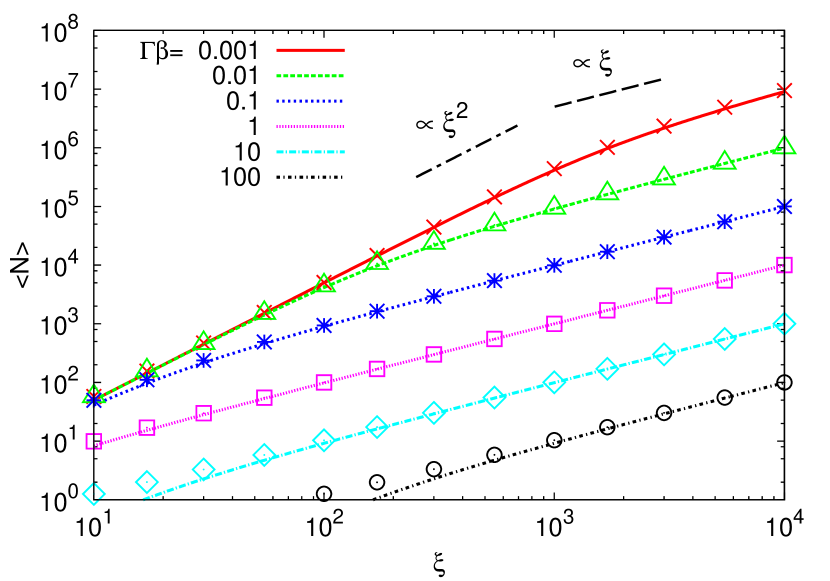
Figure 2.— The mean number of scatterings $\langle N\rangle$ for the models with $\Gamma\beta=10^{-3}$ (crosses), $10^{-2}$ (triangles), $10^{-1}$ (asterisks), 1 (squares), $10$ (diamonds), and $100$ (circles). The lines show the analytic expressions, equation (8), for the models denoted in the figure.

Figure 2 shows the mean number of scatterings $\langle N\rangle$ of $6\times 10^{3}$ photons for the models with $\Gamma\beta=10^{-3}$, $10^{-2}$, $10^{-1}$, 1 and $6\times 10^{4}$ photons for the models with $\Gamma\beta=10$ and $100$. The lines show the analytic expressions derived in the previous section with $\Gamma\beta=10^{-3},10^{-2},10^{-1},1,10$ and $100$ (Eq. (8)). This demonstrates that the analytic expressions are excellently consistent with the results of numerical simulations, except at $\langle N\rangle\sim 1$. The difference at the region comes from the fact that a considerable number of photons do not experience any scatterings in this region, although the equation (8) is obtained assuming all the photons undergo more than one scatterings.

The dependencies of $\langle N\rangle$ on $\xi$ are as follows: In the model with $\Gamma\beta=10^{-3}$, $\langle N\rangle$ is proportional to $\xi^{2}$ for $\xi<10^{3}\simeq\beta^{-1}$ and to $\xi$ for $\xi>10^{3}$. In the model with $\Gamma\beta=10^{-2}$, $\langle N\rangle$ is proportional to $\xi^{2}$ for $\xi<10^{2}$ and to $\xi$ for $\xi>10^{2}$. The transition of the dependence is at $\xi\sim\beta^{-1}$. In the models with $\Gamma\beta=10^{-1}$, 1, and $10$, $\langle N\rangle$ is proportional to $\xi$ in the range of $10<\xi<10^{4}$. In the model with $\Gamma\beta=100$, $\langle N\rangle$ is proportional to $\xi$ for $\xi>10^{2}$.

4. Summary & discussions

In this letter, we investigate the random walk process in relativistic flow. In the pure scattering medium, the mean number of scatterings at the size parameter of $\xi$ is proportional to $\xi^{2}$ for $\beta/\Gamma\ll\xi^{-1}$ and to $\xi$ for $\beta/\Gamma\gg\xi^{-1}$. These dependencies of the mean number of scatterings on $\xi$ are well reproduced by the numerical simulations. We also consider the combined scattering and absorption case. If the scattering opacity dominates the absorption opacity, the behavior of the effective optical depth is different depending on the velocity $\beta$. If $\beta\ll\sqrt{2\tau_{\rm a}/\tau_{\rm s}}$, the effective optical depth is $\tau_{*}\simeq\sqrt{\tau_{\rm a}\tau_{\rm s}/2}$ and if $\beta\gg\sqrt{2\tau_{\rm a}/\tau_{\rm s}}$, $\tau_{*}\simeq(1+\beta)\tau_{\rm a}/\beta$.

In the GRB jets, the flow has ultra-relativistic velocity ($\Gamma\gtrsim 100$) and the electron scattering opacity dominates the absorption opacity ($\tau_{\rm s}\gg\tau_{\rm a}$) due to its low density and high temperature. Thus, the effective optical depth in the jet is approximated by $\tau_{*}\simeq 2\tau_{\rm a}$. On the other hand, the cocoon have a non-relativistic velocity (e.g., Matzner, 2003) and the effective optical depth in the cocoon could be much higher than the absorption optical depth as $\tau_{*}\simeq\tau_{\rm a}/\beta\gg\tau_{\rm a}$. The effective optical depth defines the photon production site as $\tau_{*}=1$. In the subsequent papers, we will perform the radiative transfer calculations for the thermal radiation from GRB jet and cocoon taking into account the photon production at the surface of $\tau_{*}=1$. This enables us to correctly treat the photon number density at the photon production sites.

The results could be applicable not only for GRB jet and cocoon but also for the other astronomical objects such as AGNs or black hole binaries. For example, the super critical accretion flows around the black holes produce a high temperature ($\sim 10^{8}~{}\mathrm{K}$) and low density ($\sim 10^{-9}~{}\mathrm{g/cm^{3}}$) outflow with a semi-relativistic velocity ($\sim 0.1c$) (e.g., Kawashima et al., 2009). In these circumstances, the scattering process have a major role on the photon diffusion and the relativistically corrected treatment is necessary even though the flow velocity is rather small compared with the speed of light.

References

- Abramowicz et al. (1991) Abramowicz, M. A., Novikov, I. D., & Paczynski, B. 1991, ApJ, 369, 175
- Axelsson et al. (2012) Axelsson, M., Baldini, L., Barbiellini, G., et al. 2012, ApJ, 757, L31
- Bégué et al. (2013) Bégué, D., Siutsou, I. A., & Vereshchagin, G. V. 2013, ApJ, 767, 139
- Beloborodov (2010) Beloborodov, A. M. 2010, MNRAS, 407, 1033
- Beloborodov (2013) —. 2013, ApJ, 764, 157
- Giannios (2006) Giannios, D. 2006, A&A, 457, 763
- Giannios (2012) —. 2012, MNRAS, 422, 3092
- Guiriec et al. (2011) Guiriec, S., Connaughton, V., Briggs, M. S., et al. 2011, ApJ, 727, L33
- Ito et al. (2013) Ito, H., Nagataki, S., Ono, M., et al. 2013, ApJ, 777, 62
- Kawashima et al. (2009) Kawashima, T., Ohsuga, K., Mineshige, S., et al. 2009, PASJ, 61, 769
- Landau & Lifshitz (1980) Landau, L. D., & Lifshitz, E. M. 1980, Statistical physics. Pt.1, Pt.2
- Lazzati et al. (2009) Lazzati, D., Morsony, B. J., & Begelman, M. C. 2009, ApJ, 700, L47
- Lazzati et al. (2011) —. 2011, ApJ, 732, 34
- Lundman et al. (2013) Lundman, C., Pe’er, A., & Ryde, F. 2013, MNRAS, 428, 2430
- Matzner (2003) Matzner, C. D. 2003, MNRAS, 345, 575
- Mészáros & Rees (2000) Mészáros, P., & Rees, M. J. 2000, ApJ, 530, 292
- Mizuta et al. (2011) Mizuta, A., Nagataki, S., & Aoi, J. 2011, ApJ, 732, 26
- Nagakura et al. (2011) Nagakura, H., Ito, H., Kiuchi, K., & Yamada, S. 2011, ApJ, 731, 80
- Pe’er (2008) Pe’er, A. 2008, ApJ, 682, 463
- Pe’er & Ryde (2011) Pe’er, A., & Ryde, F. 2011, ApJ, 732, 49
- Rees & Mészáros (2005) Rees, M. J., & Mészáros, P. 2005, ApJ, 628, 847
- Rybicki & Lightman (1979) Rybicki, G. B., & Lightman, A. P. 1979, Radiative processes in astrophysics
- Ryde et al. (2010) Ryde, F., Axelsson, M., Zhang, B. B., et al. 2010, ApJ, 709, L172