Interference-induced enhancement of field entanglement in a microwave-driven V-type single-atom laser

Abstract

We investigate the generation and the evolution of two-mode continuous-variable (CV) entanglement from system of a microwave-driven V-type atom in a quantum beat laser. By taking into account the effects of spontaneously generated quantum interference between two atomic decay channels, we show that the CV entanglement with large mean number of photons can be generated in our scheme, and the property of the filed entanglement can be adjusted by properly modulating the frequency detuning of the fields. More interesting, it is found that the entanglement can be significantly enhanced by the spontaneously generated interference.

I Introduction

Quantum entanglement has become a fundamental resource for quantum information science, as it takes on extensive potential in the application of quantum computation and quantum communication 1 ; 2 ; 5 ; 6 ; 7 ; 8 ; 9 ; 10 ; 11 ; 12 ; 13 ; 14 . In particular, because of the relative simplicity and high efficiency in the generation, manipulation and detection of optical continuous-variable (CV) states 15 ; 16 ; 17 ; 18 , CV entanglement can offer an advantage in quantum information processing 20 , and it has been an important part of quantum information theory 20 . Therefore, more and more theoretical and experimental efforts have been devoted to the generation of CV entanglement 21 ; 24 ; 25 ; 26 ; w1 ; w2 ; w3 . Meanwhile, on the aspect of theory, Simon 27 and Duan et al 28 have proposed inseparability criterions for CV states, separately.

It has been proven to be efficient ways for generating the CV entangled beams that using of Nondegenerate parametric down conversion (NPDC) in a crystal 15 ; 29 . Besides, the preparation of the CV entangled light based on the interaction of two-mode cavity fields with atoms coherently driven by laser fields has also been investigated extensively. For example, Li et al. 30 considered the generation of two-mode entangled states of the cavity field via the four-wave mixing process, by means of the interaction of properly driven V-type three-level atoms with two cavity modes. Subsequently, Tan et al 31 extended the analysis of 30 and studied the generation and evolution of entangled light by taking into account the effects of spontaneously generated interference between two atomic decay channels. In an earlier study, Qamar et al. 32 proposed a scheme for generating of two-mode entangled states in a quantum beat laser 33 . The system consists of a V-type three-level atom interacting with two modes of the cavity field in a doubly resonant cavity, and the atom is driven into a coherent superposition of the upper two levels by a strong classical field. They numerically studied the property of entanglement for different values of Rabi frequencies in the presence of cavity losses. And Fang et al 34 extended the analysis of 32 , investigating the influence of phase and Rabi frequency of the classical driving field, cavity loss, and the purity and nonclassicality of the initial state of the cavity field on the property of the resulting two-mode entangled state. Moreover, in recent years, more and more theoretical and experimental efforts 26 ; 35 ; 36 ; 37 ; 38 have been devoted to the generation of entanglement in macroscopic light based on the single-atom laser.

Following by the work 32 and 34 , we study the generating and evolution of two-mode CV entangled states from system of V-type atom in a quantum beat laser 33 by taking into account the effects of spontaneously generated interference. In our scheme, the two transitions in the V-type atom independently interact with the two cavity modes and the two upper levels of the atom are driven by a strong classical field. We show that the CV entanglement with large mean number of photons can be generated in our scheme and by properly modulating the frequency detuning of the fields, the property of the filed entanglement can be adjusted. More interesting, it is found that the entanglement can be significantly enhanced by the spontaneously generated interference, in the given situation.

II model and master equations

Let us consider the atomic system for the quantum beat laser which is proposed by Scully and Zubairy 33 . It is consist of a three-level atom with the V configuration interacting with two (nondegenerate) cavity modes and the two upper levels of the atom are driven by a strong classical field. In Fig. 1, we show the the atomic level scheme.

The atom is pumped at a rate $\gamma_{a}$ into the level $\left|a\right\rangle$. Use a strong magnetic field with Rabi frequency $\Omega$ to drive the transition between $\left|a\right\rangle$ and $\left|b\right\rangle$, which is electric-dipole forbidden. While the two nondegenerate cavity modes of frequencies $\nu_{1}$ and $\nu_{2}$ independently interact with the transitions $\left|a\right\rangle\leftrightarrow\left|c\right\rangle$ (with $\omega_{ac}$ resonant frequency) and $\left|b\right\rangle\leftrightarrow\left|c\right\rangle$ (with $\omega_{bc}$ resonant frequency), respectively. $\Delta_{1}=\omega_{ac}-\nu_{1}$ is the detuning of the field $g_{1}$ from the corresponding atomic transition $\left|a\right\rangle\leftrightarrow\left|c\right\rangle$. $\Delta_{2}=\omega_{bc}-\nu_{2}$ is the detuning of the field $g_{2}$ from the corresponding atomic transition $\left|b\right\rangle\leftrightarrow\left|c\right\rangle$.For simplicity, we’ll note $\Delta_{1}=\Delta_{2}=\Delta$.

Figure 1: Schematic diagram of the three-level atom system in a V configuration. Two (nondegenerate) cavity modes with coupling constant $g_{1}$ and $g_{2}$ interact with the transition $\left|a\right\rangle\leftrightarrow\left|c\right\rangle$ and $\left|b\right\rangle\leftrightarrow\left|c\right\rangle$, respectively, while the atom transition $\left|a\right\rangle\leftrightarrow\left|b\right\rangle$ is driven by a strong magnetic field with Rabi frequency $\Omega$. $\Delta_{1}$ and $\Delta_{2}$ correspond the frequency detunings.

Then, under the dipole and rotating wave approximation, the total interaction Hamiltonian of our system can be given in the interaction picture by ($\hbar=1$)

$$V_{I}=\Delta\left|a\right\rangle\left\langle a\right|+\Delta\left|b\right\rangle\left\langle b\right|+(-\Omega\left|a\right\rangle\left\langle b\right|+g_{1}a_{1}\left|a\right\rangle\left\langle c\right|+g_{2}a_{2}\left|b\right\rangle\left\langle c\right|+H.c.),$$ (1)

where the symbol $H.c.$ means the Hermitian conjugate and we have taken the ground state $\left|c\right\rangle$ as the energy origin for the sake of simplicity. $\Omega=|\Omega|\exp{(i\phi)}$ describe the Rabi frequencies of the strong classical field and denote the phase of classical fields with $\phi$, and $g_{1}$ and $g_{2}$ are the atom$-$field coupling constants. $a_{j}$ ($a^{{\dagger}}_{j}$) is the annihilation (creation) operator of the corresponding cavity modes.

Considering the vacuum damping of the atom and the cavity modes, the reduced density equations of the cavity fields (taking a trace over the atom degrees of freedom 39 ) can be obtained from the Hamiltonian (1):

$$\dot{\rho}_{f} = -iTr_{atom}[V_{I},\rho]+Tr_{atom}(L_{f}\rho+L_{a}\rho)$$ (2)

$$= -ig_{1}[a_{1}^{{\dagger}},\rho_{ac}]-ig_{2}[a_{2}^{{\dagger}},\rho_{bc}]+\sum_{j=1}^{2}\kappa_{j}[a_{j},\rho_{f}a_{j}^{{\dagger}}]+H.c.,$$

with

$$L_{f}\rho=\sum_{j=1}^{2}\kappa_{j}[a_{j},\rho a_{j}^{{\dagger}}]+H.c.,$$ (3)

$$L_{a}\rho=\gamma_{1}[s_{ca},\rho s_{ac}]+\gamma_{2}[s_{cb},\rho s_{bc}]+\gamma_{12}([s_{ca},\rho s_{bc}]+[s_{cb},\rho s_{ac}])+H.c.,$$ (4)

where $L_{f}\rho$, $L_{a}\rho$ are the vacuum damping of the cavity modes and atom, respectively. $\gamma_{1}$, and $\gamma_{2}$ are the decay rates from the states $\left|a\right\rangle$ to $\left|c\right\rangle$,and $\left|b\right\rangle$ to $\left|c\right\rangle$, respectively. Meanwhile, $\gamma_{12}=P\sqrt{\gamma_{1}\gamma_{2}}$ represents the spontaneously generated interference which is resulted from the cross coupling between the transitions $\left|a\right\rangle\leftrightarrow\left|c\right\rangle$ and $\left|b\right\rangle\leftrightarrow\left|c\right\rangle$, and $P=\overrightarrow{b_{ac}}\cdot\overrightarrow{b_{bc}}/(\left|\overrightarrow{b_{ac}}\right|\cdot\left|\overrightarrow{b_{bc}}\right|)=\cos\theta$. Here $\overrightarrow{b_{ac}}$ and $\overrightarrow{b_{bc}}$ represent the atomic dipole polarizations and $\theta$ is the angle between the two dipole moments. From the expressions of the parameter P and $\gamma_{12}$ we can find that the spontaneously generated interference dependents on the angle between the two dipole moments. When the two dipole moments are perpendicular to each other the interference effect disappears (p=0), and it will be maximal (p=1) if the two dipole moments are parallel to each other. Note that $\kappa_{j}$ ($j=1,2$) are the damping constants of two cavity modes

Based on the standard methods of laser theory in 39 , considering the spontaneously decay of atom, $\rho_{ac}$ and $\rho_{bc}$ can be evaluated to the first order in the coupling constants $g_{1}$ and $g_{2}$ as

$$i\dot{\rho}_{ac}=-i\gamma_{1}\rho_{ac}-i\gamma_{12}\rho_{bc}+\Delta\rho_{ac}-\Omega\rho_{bc}-g_{1}\rho_{aa}^{(0)}a_{1}-g_{2}\rho_{ab}^{(0)}a_{2}+g_{1}a_{1}\rho_{cc}^{(0)},$$ (5)

$$i\dot{\rho}_{bc}=-i\gamma_{2}\rho_{bc}-i\gamma_{12}\rho_{ac}+\Delta\rho_{bc}-\Omega^{*}\rho_{ac}-g_{1}\rho_{ba}^{(0)}a_{1}-g_{2}\rho_{bb}^{(0)}a_{2}+g_{2}a_{2}\rho_{cc}^{(0)},$$ (6)

where the density matrix elements $\rho_{ij}^{(0)}$ can be obtained by the corresponding zeroth-order equations

$$i\dot{\rho}_{aa}^{(0)}=-2i\gamma_{1}\rho_{aa}^{(0)}-i\gamma_{12}(\rho_{ba}^{(0)}+\rho_{ab}^{(0)})-\Omega\rho_{ba}^{(0)}+\Omega^{*}\rho_{ab}^{(0)}+\Omega_{a}\rho_{f},$$ (7)

$$i\dot{\rho}_{bb}^{(0)}=-2i\gamma_{2}\rho_{bb}^{(0)}-i\gamma_{12}(\rho_{ba}^{(0)}+\rho_{ab}^{(0)})-\Omega^{*}\rho_{ab}^{(0)}+\Omega\rho_{ba}^{(0)},$$ (11)

$$i\dot{\rho}_{ab}^{(0)}=-i(\gamma_{1}+\gamma_{2})\rho_{ab}^{(0)}-i\gamma_{12}(\rho_{aa}^{(0)}+\rho_{bb}^{(0)})-\Omega\rho_{bb}^{(0)}+\Omega\rho_{aa}^{(0)},$$

$$i\dot{\rho}_{ba}^{(0)}=-i(\gamma_{1}+\gamma_{2})\rho_{ba}^{(0)}-i\gamma_{12}(\rho_{aa}^{(0)}+\rho_{bb}^{(0)})+\Omega^{*}\rho_{bb}^{(0)}-\Omega^{*}\rho_{aa}^{(0)},$$

$$i\dot{\rho}_{cc}^{(0)}=0.$$

Plugging the steady-state solution of $\rho_{ij}^{(0)}$ into Eqs. (5-6), we find the steady-state solution for $\rho_{ac}$ and $\rho_{bc}$ can be described as:

$$ig_{1}\rho_{ac}=\alpha_{11}\rho_{f}a_{1}+\alpha_{12}\rho_{f}a_{2},$$ (12)

$$ig_{2}\rho_{bc}=\alpha_{21}\rho_{f}a_{1}+\alpha_{22}\rho_{f}a_{2},$$ (13)

with the explicit expressions of the coefficients $\alpha_{ij}$ being given in Appendix. By substituting Eqs.(12-13) to the Eq. (2), the reduced master equation govern the evolution of the cavity field can be obtained as

$$\dot{\rho}_{f} = -\alpha_{11}(a_{1}^{{\dagger}}\rho_{f}a_{1}-\rho_{f}a_{1}a_{1}^{{\dagger}})-\alpha_{12}(a_{1}^{{\dagger}}\rho_{f}a_{2}-\rho_{f}a_{2}a_{1}^{{\dagger}})$$ (14)

$$-\alpha_{22}(a_{2}^{{\dagger}}\rho_{f}a_{2}-\rho_{f}a_{2}a_{2}^{{\dagger}})-\alpha_{21}(a_{2}^{{\dagger}}\rho_{f}a_{1}-\rho_{f}a_{1}a_{2}^{{\dagger}})$$

$$+\kappa_{1}(a_{1}\rho_{f}a_{1}^{{\dagger}}-\rho_{f}a_{1}^{{\dagger}}a_{1})+\kappa_{2}(a_{2}\rho_{f}a_{2}^{{\dagger}}-\rho_{f}a_{2}^{{\dagger}}a_{2})+H.c..$$

Here we remain all orders in the Rabi frequency $\Omega$ whereas only consider second order in the coupling constants $g_{1}$, $g_{2}$ due to that the coupling constants of two cavity modes are smaller than other system parameters in our scheme. Thus we can ignore the saturation effects and operate in the regime of linear amplification.

III entanglement of the cavity fields

In this section, we use the sufficient inseparability criterion proposed by Duan et al 28 . to verify that CV entanglement with large mean number of photons can be obtained in our model, and study the property of entanglement under the given conditions.

According to Duan’s criterion 28 , the two cavity modes are entangled if and only if the sum of the variances of the two Einstein-Podolsky-Rosen (EPR) type operators $\hat{u}=\hat{x}_{1}+\hat{x}_{2}$ and $\hat{v}=\hat{p}_{1}+\hat{p}_{2}$ satisfies the following inequality

$$\left\langle(\Delta\hat{u})^{2}+(\Delta\hat{v})^{2}\right\rangle<2,$$ (15)

with the pair quadrature operators $\hat{x}_{j}=(a_{j}+a_{j}^{{\dagger}})/\sqrt{2}$ and $\hat{p}_{j}=-i(a_{j}-a_{j}^{{\dagger}})/\sqrt{2}$ ($j=1,2$) the local operators which correspond to the mode at the frequency $\nu_{j}$. By substituting $\hat{x}_{j}$ and $\hat{p}_{j}$ into equation (15), we can express the total variance of the operators $\hat{u}$ and $\hat{v}$ in terms of the operators $a_{j}$ and $a_{j}^{{\dagger}}$ and achieve

$$\left\langle(\Delta\hat{u})^{2}+(\Delta\hat{v})^{2}\right\rangle = 2[1+\langle a_{1}^{{\dagger}}a_{1}\rangle+\langle a_{2}^{{\dagger}}a_{2}\rangle+\left\langle a_{1}a_{2}\right\rangle+\langle a_{1}^{{\dagger}}a_{2}^{{\dagger}}\rangle$$ (16)

$$-\left\langle a_{1}\right\rangle\langle a_{1}^{{\dagger}}\rangle-\left\langle a_{2}\right\rangle\langle a_{2}^{{\dagger}}\rangle-\left\langle a_{1}\right\rangle\left\langle a_{2}\right\rangle-\langle a_{1}^{{\dagger}}\rangle\langle a_{2}^{{\dagger}}\rangle].$$

With the help of equation (14),we can obtain the equations of motion for the expectation values of the field operators in equation (16) as

$$\frac{\partial}{\partial t}\langle a_{1}\rangle=-(\alpha_{11}+\kappa_{1})\langle a_{1}\rangle-\alpha_{12}\langle a_{2}\rangle,$$ (17)

$$\frac{\partial}{\partial t}\langle a_{2}\rangle=-(\alpha_{22}+\kappa_{2})\langle a_{2}\rangle-\alpha_{21}\langle a_{1}\rangle,$$ (18)

$$\frac{\partial}{\partial t}\langle a_{1}^{{\dagger}}\rangle=-(\alpha_{11}^{*}+\kappa_{1})\langle a_{1}^{{\dagger}}\rangle-\alpha_{12}^{*}\langle a_{2}^{{\dagger}}\rangle,$$ (19)

$$\frac{\partial}{\partial t}\langle a_{2}^{{\dagger}}\rangle=-(\alpha_{22}^{*}+\kappa_{2})\langle a_{2}^{{\dagger}}\rangle-\alpha_{21}^{*}\langle a_{1}^{{\dagger}}\rangle,$$ (20)

$$\frac{\partial}{\partial t}\langle a_{1}^{{\dagger}}a_{1}\rangle=-(\alpha_{11}+\alpha_{11}^{*}+2\kappa_{1})\langle a_{1}^{{\dagger}}a_{1}\rangle-\alpha_{12}\langle a_{1}^{{\dagger}}a_{2}\rangle-\alpha_{12}^{*}\langle a_{1}a_{2}^{{\dagger}}\rangle-(\alpha_{11}+\alpha_{11}^{*}),$$ (21)

$$\frac{\partial}{\partial t}\langle a_{2}^{{\dagger}}a_{2}\rangle=-(\alpha_{22}+\alpha_{22}^{*}+2\kappa_{2})\langle a_{2}^{{\dagger}}a_{2}\rangle-\alpha_{21}^{*}\langle a_{1}^{{\dagger}}a_{2}\rangle-\alpha_{21}\langle a_{1}a_{2}^{{\dagger}}\rangle-(\alpha_{22}+\alpha_{22}^{*}),$$ (22)

$$\frac{\partial}{\partial t}\langle a_{1}^{{\dagger}}a_{2}\rangle=-\alpha_{21}\langle a_{1}^{{\dagger}}a_{1}\rangle-\alpha_{12}^{*}\langle a_{2}^{{\dagger}}a_{2}\rangle-(\alpha_{11}^{*}+\alpha_{22}+\kappa_{1}+\kappa_{2})\langle a_{1}^{{\dagger}}a_{2}\rangle-(\alpha_{12}^{*}+\alpha_{21}),$$ (23)

$$\frac{\partial}{\partial t}\langle a_{1}a_{2}^{{\dagger}}\rangle=-\alpha_{21}^{*}\langle a_{1}^{{\dagger}}a_{1}\rangle-\alpha_{12}\langle a_{2}^{{\dagger}}a_{2}\rangle-(\alpha_{11}+\alpha_{22}^{*}+\kappa_{1}+\kappa_{2})\langle a_{1}a_{2}^{{\dagger}}\rangle-(\alpha_{12}+\alpha_{21}^{*}),$$ (24)

$$\frac{\partial}{\partial t}\langle a_{1}a_{2}\rangle=-\alpha_{21}\langle a_{1}a_{1}\rangle-\alpha_{12}\langle a_{2}a_{2}\rangle-(\alpha_{11}+\alpha_{22}+\kappa_{1}+\kappa_{2})\langle a_{1}a_{2}\rangle,$$ (25)

$$\frac{\partial}{\partial t}\langle a_{1}a_{1}\rangle=-2(\alpha_{11}+\kappa_{1})\langle a_{1}a_{1}\rangle-2\alpha_{12}\langle a_{1}a_{2}\rangle,$$ (26)

$$\frac{\partial}{\partial t}\langle a_{2}a_{2}\rangle=-2(\alpha_{22}+\kappa_{2})\langle a_{2}a_{2}\rangle-2\alpha_{21}\langle a_{1}a_{2}\rangle,$$ (27)

$$\frac{\partial}{\partial t}\langle a_{1}^{{\dagger}}a_{2}^{{\dagger}}\rangle=-\alpha_{21}^{*}\langle a_{1}^{{\dagger}}a_{1}^{{\dagger}}\rangle-\alpha_{12}^{*}\langle a_{2}^{{\dagger}}a_{2}^{{\dagger}}\rangle-(\alpha_{11}^{*}+\alpha_{22}^{*}+\kappa_{1}+\kappa_{2})\langle a_{1}^{{\dagger}}a_{2}^{{\dagger}}\rangle,$$ (28)

$$\frac{\partial}{\partial t}\langle a_{1}^{{\dagger}}a_{1}^{{\dagger}}\rangle=-2(\alpha_{11}^{*}+\kappa_{1})\langle a_{1}^{{\dagger}}a_{1}^{{\dagger}}\rangle-2\alpha_{12}^{*}\langle a_{1}^{{\dagger}}a_{2}^{{\dagger}}\rangle,$$ (29)

$$\frac{\partial}{\partial t}\langle a_{2}^{{\dagger}}a_{2}^{{\dagger}}\rangle=-2(\alpha_{22}^{*}+\kappa_{2})\langle a_{2}^{{\dagger}}a_{2}^{{\dagger}}\rangle-2\alpha_{21}^{*}\langle a_{1}^{{\dagger}}a_{2}^{{\dagger}}\rangle.$$ (30)

By numerically solving these equations, we can give a few numerical results for the time evolution of the total photon numbers $\langle\hat{N}\rangle=\langle a_{1}^{{\dagger}}a_{1}\rangle+\langle a_{2}^{{\dagger}}a_{2}\rangle$ and $\left\langle(\Delta\hat{u})^{2}+(\Delta\hat{v})^{2}\right\rangle$ with different values of parameter while the cavity modes are assumed to be in the coherent state $\left|10,-10\right\rangle$, as illustrated in Figs. 2-4. It is easy to find that, the CV entanglement with large mean number of photons from system of V-type atom in a quantum beat laser can be generated, and the entanglement can be enhanced by the spontaneously generated interference. For simplicity, all the parameters used here are scaled with $g$, and we have chosen $\phi=\pi/2$ during our numerical calculations.

By above knowable, $\gamma_{12}=P\sqrt{\gamma_{1}\gamma_{2}}$ represents the spontaneously generated interference. Therefore, in order to check the effect of the spontaneously generated interference on the time evolution of entanglement, we can study the property of entanglement for different values of atomic decay rates and the parameter P.

In Fig. 2, we show the plot of the time development of $\langle(\Delta\hat{u})^{2}+(\Delta\hat{v})^{2}\rangle$ and $\langle\hat{N}\rangle$ for different values of atomic decay rates, when the cavity field is initially in the coherent state $\left|10,-10\right\rangle$. From Fig. 2(a), one can find that the intensity and period of entanglement can be enlarged by increasing spontaneous emission decay rates of the atom level, while Fig. 2(b) illustrates that the effect of the atomic decay rates $\gamma_{j}$ ($j=1,2$) on the maximum mean photon numbers give a small extent.

Figure 2: The time evolution of $\langle(\Delta\hat{u})^{2}+(\Delta\hat{v})^{2}\rangle$ (shown in Fig. 2(a)) and the total mean photon numbers $\langle\hat{N}\rangle$ (shown in Fig. 2(b)) for different atomic decay rates $\gamma$ ($\gamma_{1}=\gamma_{2}=\gamma$), when the cavity field is initially in the coherent state $\left|10,-10\right\rangle$. The other parameters are $\kappa_{1}=\kappa_{2}=0.001g$, $P=0.5$, $|\Omega|=10g$, $\Delta_{1}=\Delta_{2}=\Delta=g$, $\gamma_{a}=5g$ and $\phi=\pi/2$.

Figure 3: The time evolution of $\langle(\Delta\hat{u})^{2}+(\Delta\hat{v})^{2}\rangle$ (shown in Fig. 3(a)) and the total mean photon numbers $\langle\hat{N}\rangle$ (shown in Fig. 3(b)) different values of P, when the cavity field is initially in the coherent state $\left|10,-10\right\rangle$. The other parameters are $\kappa_{1}=\kappa_{2}=0.001g$, $\gamma_{1}=\gamma_{2}=\gamma=g$, $|\Omega|=10g$, $\Delta_{1}=\Delta_{2}=\Delta=g$, $\gamma_{a}=5g$ and $\phi=\pi/2$.

In order to check the influence of P on the entanglement property, we numerically simulate the time evolution of $\langle(\Delta\hat{u})^{2}+(\Delta\hat{v})^{2}\rangle$ and $\langle\hat{N}\rangle$ for different values of P. As shown in Fig. 3(a), when the cavity field is initially in coherent state $\left|10,-10\right\rangle$, the intensity of entanglement between the two cavity modes slightly enhances with the increase of the value of P. With the same set of the parameters, Fig. 3(b) shows that the maximum mean photon numbers $\langle\hat{N}\rangle$ become more pronounced with the increase of the value of P.

Up to now, we have investigated the the influence of spontaneous emission decay rates of the atom level and the parameter P on the time evolution of entanglement. It is easy to find that, the entanglement can be enhanced by no matter increasing the spontaneous emission decay rates of the atom level or increasing the value of P. Then we conclude that, the spontaneously generated interference which depends on $\gamma_{j}$ ($j=1,2$) and P, can strengthen the entanglement.

We plot the influence of frequency detuning of the cavity field on the time evolution of entanglement under condition that the cavity field is initially in the coherent state $\left|10,-10\right\rangle$ (shown in Fig. 4). As shown in Fig. 4(a) that the intensity and period of entanglement between the two cavity modes can be enlarged at one time by decreasing the frequency detuning of the pump field $\Delta$($\Delta_{1}=\Delta_{2}=\Delta$). In addition, Fig. 4(b) illustrate that with the increased of the detuning $\Delta$, the maximum mean photon number is enlarged. This result implicates that in order to obtain the entanglement of cavity modes with high intensity and longer period we can do that by properly adjusting the frequency detuning.

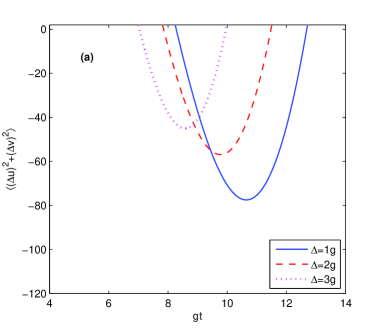
Figure 4: The time evolution of $\langle(\Delta\hat{u})^{2}+(\Delta\hat{v})^{2}\rangle$ (shown in Fig.4(a)) and the total mean photon numbers $\langle\hat{N}\rangle$ (shown in Fig. 4(b)) for different frequency detuning $\Delta$($\Delta_{1}=\Delta_{2}=\Delta$), when the cavity field is initially in the coherent state $\left|10,-10\right\rangle$. The other parameters are $\gamma_{1}=\gamma_{2}=g$, $\kappa_{1}=\kappa_{2}=0.001g$, $P=0.5$, $|\Omega|=10g$, $\gamma_{a}=5g$ and $\phi=\pi/2$.

Before conclusion, we should note that our scheme is drastically different from the conventional scheme of CV entanglement generation 32 ; 34 . In our scheme, with decreasing the frequency detuning, our numerical results showed that a long entanglement time and strong entanglement intensity can be synchronously achieved. It illustrates that the entanglement of cavity modes with higher intensity and longer period can be realized in our scheme with a low-Q cavity. And it can strengthen the entanglement by increasing the spontaneous emission decay rates of the atom level and the value of the parameter P. The physical reason can be explained that no matter larger the atom decay rates $\gamma_{j}$ ($j=1,2$) or larger the value of P results in increasing the spontaneously generated interference which can enhance the entanglement. All these distinguish advances illustrate that our scheme is drastically different from the conventional scheme.

IV conclusion

In summary, we have proposed a new scheme to generate the CV entanglement and investigated the evolution of it from a system of V-type atom in a quantum beat laser 33 . In this scheme, the two transitions in the V-type atom independently interact with the two cavity modes while the two upper levels of the atom are driven by a strong classical field. By taking into account the effects of spontaneously generated interference between two atomic decay channels, and using the standard methods of laser theory 39 , we show that, in the given conditions, the CV entanglement with large mean number of photons can be realized in our scheme. And by properly modulating the frequency detuning of the field can adjust the entanglement period, intensity and the total mean photon numbers of two cavity modes. Different from the conventional scheme 32 ; 34 , the CV entanglement of cavity modes with higher intensity and longer period can be realized in our scheme with a low-Q cavity. Furthermore, our results showed that the entanglement can be significantly enhanced by the spontaneously generated interference.

We would like to thank Prof. Peng Xue for her enlightening discussions. The research is supported in part by National Natural Science Foundation of China under Grant Nos. 11374050 and 61372102, by Qing Lan project of Jiangsu, and by the Fundamental Research Funds for the Central Universities under Grant No. 2242012R30011.

Appendix A coefficients

Here we give the expressions of the coefficients $A_{ij}$ and $B_{ij}$ ($i,j=1,2$) in Eqs. (12-14),

$$\alpha_{11}=-g_{1}^{2}[(R+i\Delta)\beta_{aa}+(i\Omega-\gamma_{12})\beta_{ba}]/D_{1},$$ (37)

$$\alpha_{12}=-g_{1}g_{2}[(R+i\Delta)\beta_{ab}+(i\Omega-\gamma_{12})\beta_{bb}]/D_{1},$$

$$\alpha_{22}=-g_{2}^{2}[(R+i\Delta)\beta_{bb}+(i\Omega^{*}-\gamma_{12})\beta_{ab}]/D_{1},$$

$$\alpha_{21}=-g_{1}g_{2}[(R+i\Delta)\beta_{ba}+(i\Omega^{*}-\gamma_{12})\beta_{aa}]/D_{1},$$

$$\beta_{aa}=(2R^{2}-\gamma_{12}^{2}+|\Omega|^{2})R\gamma_{a}/D_{2},$$

$$\beta_{bb}=(\gamma_{12}+i\Omega)(\gamma_{12}-i\Omega^{*})R\gamma_{a}/D_{2},$$

$$\beta_{ab}=-(\gamma_{12}+i\Omega)(2R^{2}-i\gamma_{12}\Omega-i\gamma_{12}\Omega^{*})R\gamma_{a}/(2D_{2}),$$

$$\beta_{ba}=-(\gamma_{12}-i\Omega^{*})(2R^{2}+i\gamma_{12}\Omega+i\gamma_{12}\Omega^{*})R\gamma_{a}/(2D_{2}),$$ (38)

with

$$D_{1} = (R+i\Delta)^{2}-(i\Omega-\gamma_{12})(i\Omega^{*}-\gamma_{12}),$$ (39)

$$D_{2} = 4R^{4}+4R^{2}|\Omega|^{2}-4R^{2}\gamma_{12}^{2}-\gamma_{12}^{2}(\Omega+\Omega^{*})^{2},$$ (40)

where we have assumed $\gamma_{1}=\gamma_{2}=\gamma=R$.

References

• (1) C. H. Bennett, G. Brassard, C. Crepeau, R. Jozsa, A. Peres, W. K. Wootters, Phys. Rev. Lett. 70 (1993) 1895.
• (2) D. Bouwmeester, J. W. Pan, K. Mattle, M. Eibl, H. Weinfurter, A. Zeilinger, Nature 390 (1997) 575.
• (3) D. P. Divincerzo, Science 270 (1995) 225.
• (4) M. Feng, Phys. Rev. A 66 (2002) 054303.
• (5) S. B. Zheng, G. C. Guo, Phys. Rev. A 73 (2006) 032329.
• (6) Y. Wu, L. L. Wen, Y. F. Zhu, Opt. Lett. 28 (2003) 631.
• (7) Y. Wu, X. X. Yang, Appl. Phys. Lett. 91 (2007) 094104.
• (8) Y. Wu, X. X. Yang, Opt. Lett. 28 (2003) 1793.
• (9) W. X. Yang, Z. M. Zhan, J. H. Li, Phys. Rev. A 72 (2005) 062108.
• (10) W. X. Yang, X. L. Gong, J. H. Li, L. X. Jin, Phys. Rev. A 70 (2004) 033812.
• (11) W. X. Yang, R. K. Lee, Opt. Express 16 (2008) 17161.
• (12) X. Y. Lü, P. Huang, W. X. Yang, X. X. Yang, Phys. Rev. A 80 (2009) 032305.
• (13) Z. Y. Ou, S. F. Pereira, H. J. Kimble, K. C. Peng, Phys. Rev. Lett. 68 (1992) 3663.
• (14) S. L. Braunstein, H. J. Kimble, Phys. Rev. Lett. 80 (1998) 869.
• (15) X. Y. Li, Q. Pan, J. T. Jing, J. Zhang, C. D. Xie, K. C. Peng, Phys. Rev. Lett. 88 (2002) 047904.
• (16) S. Lloyd, S. L. Braunstein, Phys. Rev. Lett. 82 (1999) 1784.
• (17) S. L. Braunstein, P. V. Loock, Rev. Mod. Phys. 77 (2005) 513.
• (18) G. X. Li, S. P. Wu, G. M. Huang, Phys. Rev. A 71 (2005) 063817.
• (19) G. X. Li, Y. P. Yang, K. Allaart, D. Lenstra, Phys. Rev. A 69 (2004) 014301.
• (20) H. Xiong, M. O. Scully, M. S. Zubairy, Phys. Rev. Lett. 94 (2005) 023601.
• (21) M. Kiffner, M. S. Zubairy, J. Evers, C. H. Keitel, Phys. Rev. A 75 (2007) 033816.
• (22) Y. Wu, M.G. Payne, E.W. Hageley, and L. Deng, Phys. Rev. A 69, 063803 (2004).
• (23) Y. Wu, M.G. Payne, E.W. Hageley, and L. Deng, Phys. Rev. A 70, 063812 (2004).
• (24) Y. Wu and X. Yang, Appl. Phys. Lett. 91, 094104 (2007).
• (25) R. Simon, Phys. Rev. Lett. 84 (2000) 2726.
• (26) L. M. Duan, G. Giedke, J. I. Cirac, P. Zoller, Phys. Rev. Lett. 84 (2000) 2722.
• (27) X. J. Jia, X. L. Su, Q. Pan, J. R. Gao, C. D. Xie, K. C. Peng, Phys. Rev. Lett. 93 (2004) 250503.
• (28) G. X. Li, H. T. Tan, M. Macovei, Phys. Rev. A 76 (2007) 053827.
• (29) H. T. Tan, H. X. Xia, G. X. Li, Phys. Rev. A 79 (2009) 063805.
• (30) S. Qamar, F. Ghafoor, M. Hillery, M. S. Zubairy, Phys. Rev. A 77 (2008) 062308.
• (31) M. O. Scully, M. S. Zubairy, Phys. Rev. A 35 (1987) 752.
• (32) A. P. Fang, Y. L. Chen, F. L. Li, H. R. Li, P. Zhang, Phys. Rev. A 81 (2010) 012323.
• (33) X. Y. Lü, J. B. Liu, L. G. Si, X. X. Yang, J. Phys. B: At. Mol. Opt. Phys. 41 (2008) 035501.
• (34) L. Zhou, H. Xiong, M. S. Zubairy, Phys. Rev. A 74 (2006) 022321.
• (35) B. B. Blinov, D. L. Moehring, L. M. Duan, C. Monroe, Nature 428 (2004) 153.
• (36) G. Morigi, J. Eschner, S. Mancini, D. Vitali, Phys. Rev. Lett. 96 (2006) 023601.
• (37) M. O. Scully, M. S. Zubairy, Quantum Optics , Cambridge: Cambridge University Press, 1997, p 409.