A numerical method to calculate the muon relaxation function in the presence of diffusion

Abstract

We present an accurate and efficient method to calculate the effect of random fluctuations of the local field at the muon, for instance in the case muon diffusion, within the framework of the strong collision approximation. The method is based on a reformulation of the Markovian process over a discretized time base, leading to a summation equation for the muon polarization function which is solved by discrete Fourier transform. The latter is formally analogous, though not identical, to the integral equation of the original continuous-time model, solved by Laplace transform. With real-case parameter values, the solution of the discrete-time strong collision model is found to approximate the continuous-time solution with excellent accuracy even with a coarse-grained time sampling. Its calculation by the fast Fourier transform algorithm is very efficient and suitable for real time fitting of experimental data even on a slow computer.

I Introduction

One of the greatest benefits of muon spin rotation ($\mu$SR) as a local probe of magnetism in condensed matter is its capability of detecting randomly distributed static magnetic fields even in the absence of a net bias field. This makes $\mu$SR the technique of choice for the study of disordered magnets or weakly magnetic systems, such as spin and cluster-spin glasses. In most cases, purely static magnetic disorder is adequately accounted for by a classical distribution of random fields, whence the longitudinal muon spin polarization function $G(t)\equiv\left\langle{S_{z}(t)S_{z}(0)}\right\rangle/\left\langle{S_{z}(0)^{2}}\right\rangle$ is calculated by averaging the precession waveform of a muon in a random local field over the muon ensemble. For instance a Gaussian distribution, yielding the well-known static Kubo-Toyabe function, Kubo and Toyabe (1967) suitably describes the muon depolarization by the static dipolar fields of nuclei.

The effect of time-dependent fluctuations on an otherwise static random distribution of fields at the muon can be easily accounted for in the limit of very rapid fluctuations (the so-called narrowing limit), whereby they produce simple exponential muon spin relaxations. The intermediate case between the narrowing limit and purely static fields requires however a detailed modelling of the dynamical processes perturbing the instantaneous field at the muon. The simplest dynamical model, suitable e.g. to describe the effect of muon diffusion, is based on a strong collision approximation, Kubo (1954) dealing with the muon spin evolution in the form of a Markovian process. Such a model yields a recursion series for $G(t)$, whose summation leads to an integral equation, which is solved in principle by Laplace transform. Hayano et al. (1979) However, an exact analytical solution of the strong collision model (SCM) with an arbitrary distribution of static fields cannot be obtained. In the most general case, including that of a Gaussian distribution corresponding to the dynamical Kubo-Toyabe function, Laplace transforms have to be calculated and inverted numerically. This makes the Laplace transform method impractical, especially when the free parameters of the model have to be optimized in order to fit experimental data. To overcome these difficulties, approximate solutions of the SCM, valid in a limited range of parameters, have been obtained. Kehr et al. (1978); Keren (1994)

In this paper we illustrate an effective method, alternative to both numerical quadrature and approximate solutions, to solve the SCM and calculate $G(t)$ for a generic static field distribution. The basic idea underlying the method is replacing Laplace integrals with discrete Fourier transforms (DFT). However, the naive replacement of continuous-variable integrals with discrete sums, as proposed by Weber al., Weber et al. (1994) leads to badly inaccurate results. In order to correctly transpose the original integral equation into a summation equation, we recalculated the Markov chains directly and self-consistently over a discretized time base $t_{n}$, in a so-called discrete-time SCM (DTSCM). The solution of the resulting equation by DFT provides an efficient and accurate algorithm to calculate $G(t_{n})$, suitable for real time fitting of experimental data.

The paper is organized as follows. The continuous-time SCM is recalled for reference in section II. Its reformulation into a DTSCM is detailed in section III. The application of the DTSCM as an effective calculation method is discussed in section IV.

II The strong collision model

We recall here briefly the results of the original SCM applied to the muon spin evolution in a randomly distributed local field, due to Hayano et al. Hayano et al. (1979) The model postulates that after a “collision” event, occurring with a probability $\nu$ per unit time, the local field is a random variable totally uncorrelated with the local field before the collision, and governed by the same distribution (i.e. collisions map the static field distribution into itself). Based on these assumptions, it is legitimate to treat the muon spin ensemble, described by its polarization function $G(t)$, as a single entity subject to collisions as a whole. Hayano et al. (1979); Kehr et al. (1978) $G(t)$ will then evolve as the unperturbed static-field function $G^{(0)}(t)$ with probability $\exp(-\nu t)$, corresponding to no scattering event in the $[0,t]$ time interval; or it will resume as $G^{(0)}(t_{1})G^{(0)}(t-t_{1})$ with probability $\lambda\exp(-\nu t){\rm d}t_{1}$ after a collision occurred in a time interval ${\rm d}t_{1}$ around $t_{1}$, and so on. This leads to the following expansion in powers of $\nu$:

$${}G(t) = {\rm e}^{-\nu t}G^{(0)}(t)\,+$$ (1)

$$\mskip-40.0mu\nu\mskip 0.0mu\int_{0}^{t}\mskip-6.0mu{\rm d}t_{1}\mskip 4.0mu{\rm e}^{\nu t_{1}}G^{(0)}(t_{1})\,{\rm e}^{\nu(t-t_{1})}G^{(0)}(t-t_{1})\,+$$

$$\mskip-40.0mu\nu^{2}\mskip-6.0mu\int_{0}^{t}\mskip-6.0mu{\rm d}t_{1}\mskip 4.0mu{\rm e}^{\nu t_{1}}G^{(0)}(t_{1})\cdot$$

$$\mskip-40.0mu~{}\int_{t_{1}}^{t}\mskip-6.0mu{\rm d}t_{2}\mskip 4.0mu{\rm e}^{\nu(t_{2}-t_{1})}G^{(0)}(t_{2}-t_{1})\,{\rm e}^{\nu(t-t_{2})}G^{(0)}(t-t_{2})$$

$$\mskip-40.0mu\,+~{}\dots$$

which is rewritten into the following recursion series, upon changing the order of integration:

$${}G(t) = {\rm e}^{-\nu t}G^{(0)}(t)+\nu\mskip-6.0mu\int_{0}^{t}\mskip-6.0mu{\rm d}t_{1}{\rm e}^{-\nu(t-t_{1})}G^{(0)}(t-t_{1})\cdot$$ (2)

$$\mskip-40.0mu\left\{{\rm e}^{-\nu t_{1}}G^{(0)}(t_{1})+\nu\mskip-6.0mu\int_{0}^{t_{1}}\mskip-6.0mu{\rm d}t_{2}\mskip 4.0mu{\rm e}^{-\nu(t_{1}-t_{2})}G^{(0)}(t_{1}-t_{2})\right.\cdot$$

$$\mskip-40.0mu~{}\left.\left[\,{\rm e}^{-\nu t_{2}}G^{(0)}(t_{2})+\nu\mskip-6.0mu\int_{0}^{t_{2}}\mskip-6.0mu{\rm d}t_{3}\dots\right]\cdot\quad\dots\quad\right\}.$$

From the comparison with the right hand side of Eq. (2), it is apparent that the expression in braces equals $G(t_{1})$. Defining $H^{(0)}(t)\equiv G^{(0)}(t)\exp(-\nu t)$, the following Dyson-type integral equation is obtained for $G(t)$:

$${}G(t)=H^{(0)}(t)+\nu\mskip-6.0mu\int_{0}^{t}\mskip-6.0mu{\rm d}t_{1}\mskip 4.0muH^{(0)}(t-t_{1})\,G(t_{1})$$ (3)

or

$${}G=H^{(0)}+\nu\,H^{(0)}\mskip-6.0mu\ast G$$ (4)

where the convolution operator “$\ast$” is defined as the integral in the rightmost term of Eq. (3), i.e. as in the theory of Laplace transform. Equation (4) is solved in principle by Laplace transformation. Let ${\cal H}^{(0)}(s)\equiv{\cal L}_{s}\{H^{(0)}\}$, ${\cal G}^{(0)}(s)\equiv{\cal L}_{s}\{G^{(0)}\}$, ${\cal G}(s)\equiv{\cal L}_{s}\{G\}$ be the Laplace transforms of $H^{(0)}(t)$, $G^{(0)}(t)$ and $G(t)$, respectively; then Hayano et al. (1979)

$${}{\cal G}(s)=\frac{{\cal H}^{(0)}(s)}{1-\nu{\cal H}^{(0)}(s)}=\frac{{\cal G}^{(0)}(s+\nu)}{1-\nu{\cal G}^{(0)}(s+\nu)}~{}.$$ (5)

An analytical expression for $G(t)$ can be obtained from Eq. (5) in the case of a Lorentzian distribution of random static fields in zero external field, corresponding to a Lorentzian Kubo-Toyabe polarization function Kubo (1981)

$${}G_{\rm L}^{(0)}(t)=\frac{1}{3}+\frac{2}{3}(1-\Lambda t)\,{\rm e}^{-\Lambda t}$$ (6)

where $\Lambda/\gamma_{\mu}$ is the distribution half width ($\gamma_{\mu}$ is the muon gyromagnetic ratio). Its Laplace transform is straightforwardly calculated as

$${}{\cal G}_{\rm L}^{(0)}(s)=\frac{1}{3s}+\frac{2}{3(s+\Lambda)}-\frac{2}{3(s+\Lambda)^{2}}~{}.$$ (7)

From Eq. (5) andEq. (7), the $s$-domain dynamic function ${\cal G}_{\rm L}(s)$ is a third-order rational function with non-degenerate poles $P_{k}(\nu,\Lambda)$ for $\nu\neq 0$, which is decomposed into a sum of simple fractions of the form

$${}{\cal G}_{\rm L}(s)=\sum_{k=1}^{3}\,\frac{C_{k}(\nu,\Lambda)}{s-P_{k}(\nu,\Lambda)}$$ (8)

whence the time-domain function $G_{\rm L}(t)$ is the superposition of three exponentials,

$${}G_{\rm L}(t)=\sum_{k=1}^{3}C_{k}\,{\rm e}^{P_{k}t}~{}.$$ (9)

The application of the SCM to a Lorentzian random field distribution is a rather academic exercise. Here, the main interest of Eq. (9) is providing an exact solution of the continuous-time SCM to be used as a benchmark for the DTSCM developed in the next section. In most situations of practical interest the field distribution is instead Gaussian, as in the case of the stray dipolar fields from nuclei, which produce a muon depolarization following the static Kubo-Toyabe function Kubo and Toyabe (1967) at low temperature,

$${}G_{\rm KT}^{(0)}(t)=\frac{1}{3}+\frac{2}{3}(1-\Delta^{2}\,t)\,{\rm e}^{-\frac{1}{2}\Delta^{2}\,t^{2}}$$ (10)

where $(\Delta/\gamma_{\mu})^{2}$ is the second moment of each Cartesian component of the local field. Schenck (1985) In this context the SCM correctly describes the effect of the thermally activated diffusion of the muon on its relaxation function. However, an analytic expression for the dynamic Kubo-Toyabe function $G_{\rm KT}(t)$ analogous to Eq. (9) cannot be obtained from Eq. (10) and Eq. (5), therefore $G_{\rm KT}(t)$ has to be calculated numerically.

III The discrete-time strong collision model

We now modify the original SCM sketched in the previous section I, by imposing that scattering events may occur only at discrete times $t_{n}=n\tau$, where $n$ is an integer. Let $\lambda$ be the probability that a collision occurs over the finite time lag $\tau$, and $q=1-\lambda$ the complementary probability. According to the above definitions, $\lambda=1-\exp(-\nu\tau)$, while the probability that no collision occurs over a time $t_{n}$ equals $q^{n}=\exp(-n\nu\tau)$. Following a similar argument as for the continuous-time case, the muon spin polarization $G_{n}\equiv G(t_{n})$ will be the unperturbed $G_{n}^{(0)}$ with probability $q^{n}$; or it will be given by the free evolution to $t_{k}$ with probability $q^{k-1}$, followed by the free evolution to $t_{n}$ with probability $q^{n-k}$, in the case of single collision occurred at a non-zero time $t_{k}\leq t_{n}$ with probability $\lambda$, each $k$ thus contributing a term $G_{n-k}^{(0)}G_{k}^{(0)}$ with probability $\lambda q^{n-1}$; and so on. We are thus led to write the following equations for the Markov chain:

$${}G_{0} = G_{0}^{(0)}=1$$

$${}G_{1} = q^{1}G_{1}^{(0)}+\lambda q^{0}G_{1}^{(0)}\cdot q^{0}G_{0}^{(0)}$$

$${}G_{2} = q^{2}G_{2}^{(0)}+\lambda\left(q^{0}G_{1}^{(0)}\cdot q^{1}G_{1}^{(0)}+q^{1}G_{2}^{(0)}\cdot q^{0}G_{0}^{(0)}\right)+$$

$$\mskip-28.0mu\lambda^{2}q^{0}G_{1}^{(0)}\cdot q^{0}G_{1}^{(0)}\cdot q^{0}G_{0}^{(0)}$$

$${}\dots\mskip-1.0mu$$

$${}G_{n} = q^{n}G_{n}^{(0)}+\lambda\sum_{k=0}^{n-1}q^{k}G_{k+1}^{(0)}\cdot q^{n-k-1}G_{n-k-1}^{(0)}+$$ (11)

$$\mskip-28.0mu\lambda^{2}\sum_{k=0}^{n-1}q^{k}G_{k+1}^{(0)}\mskip-6.0mu\sum_{h=0}^{n-k-2}q^{h}G_{h+1}^{(0)}\cdot q^{n-k-h-2}G_{n-k-h-2}^{(0)}+$$

$$\mskip-28.0mu\,\dots$$

Defining $H_{n}^{(0)}\equiv q^{n}G_{n}^{(0)}=G_{n}^{(0)}\exp(-n\nu\tau)$ as in the continuous time case, and taking into account that $H_{0}^{(0)}=1$, equation Eq. (III) is straightforwardly rewritten as

$${}\mskip-48.0muG_{n} = H_{n}^{(0)}+\frac{\lambda}{q}\sum_{k=0}^{n-1}H_{k+1}^{(0)}H_{n-k-1}^{(0)}+$$ (12)

$$\mskip-40.0mu\left(\frac{\lambda}{q}\right)^{\!\!2}\,\sum_{k=0}^{n-1}\mskip 6.0mu\sum_{h=0}^{n-k-2}H_{k+1}^{(0)}H_{h+1}^{(0)}H_{n-k-h-2}^{(0)}+\,\dots$$

whence, upon factoring the outermost summation, a recursive series is obtained, analogous of Eq. (2)

$${}\mskip 0.0muG_{n} = H_{n}^{(0)}+\frac{\lambda}{q}\sum_{k=0}^{n-1}H_{k+1}^{(0)}\left\{H_{n-k-1}^{(0)}+\phantom{\left(\frac{\lambda}{q}\right)^{\!\!2}\,\sum_{h=0}^{n-k-2}\mskip-40.0mu\sum_{j=0}^{n-k-h-3}\mskip-260.0muH_{h+1}^{(0)}H_{j+1}^{(0)}H_{n-k-h-j-3}^{(0)}}\right.$$

$$\mskip-32.0mu\frac{\lambda}{q}\sum_{h=0}^{n-k-2}\mskip-6.0muH_{h+1}^{(0)}H_{n-k-h-2}^{(0)}\,+$$

$$\mskip-40.0mu\left.\left(\frac{\lambda}{q}\right)^{\!\!2}\,\sum_{h=0}^{n-k-2}\mskip-16.0mu\sum_{j=0}^{\mskip 28.0mun-k-h-3}\mskip-16.0muH_{h+1}^{(0)}H_{j+1}^{(0)}H_{n-k-h-j-3}^{(0)}\,+\dots\right\}.$$

Upon recognizing that the expression within braces in Eq. (III) equals the expansion for $G_{n-k-1}$ as of Eq. (12), we obtain the following summation equation

$${}G_{n} = H_{n}^{(0)}+\frac{\lambda}{q}\sum_{k=1}^{n}H_{k}^{(0)}G_{n-k}=$$ (14)

$$H_{n}^{(0)}+\frac{\lambda}{q}\sum_{k=0}^{n}(H_{k}^{(0)}-\delta_{k,0})G_{n-k}$$

or

$${}G=H^{(0)}+\frac{\lambda}{q}\,\mbox{\rm conv}\!\left(H^{(0)}\!-\delta,G\right)$$ (15)

where $\delta_{n}\equiv\delta_{n,0}$, and the $\mbox{\rm conv}()$ operator is defined as

$${}\mbox{\rm conv}(A,B)_{n}\equiv\sum_{k=0}^{n}A_{k}B_{n-k}$$ (16)

formally analogous to the the convolution operator “$\ast$” defined in section II.

Equation (14) (as well as its continuos-variable counterpart Eq. (3)) exhibits a remarkable invariance by exponential weighting. Let $G$ be the solution of Eq. (14); then, the same equation holds also for the exponentially weighted quantities $\tilde{H}_{n}^{(0)}\equiv H_{n}^{(0)}\exp(-\alpha n)$, $\tilde{G}_{n}\equiv G_{n}\exp(-\alpha n)$:

$${}{\tilde{G}}={\tilde{H}}^{(0)}+\frac{\lambda}{q}\,\mbox{\rm conv}\!\left({\tilde{H}}^{(0)}\!-\delta,{\tilde{G}}\right).$$ (17)

Despite the formal similarity between equations Eq. (4) and Eq. (15), an exact closed expression in terms of $H^{(0)}$, analogous to Eq. (5), cannot be obtained for the discrete time case. Indeed, the $\mbox{\rm conv}()$ operator defined in Eq. (16) is not transformed into a product by DFT (denoted hereafter as ${\cal F}\left\{{}\right\}$). Rather, it is circular convolution, defined as

$${}(A\ast B)_{n}\equiv\sum_{k=0}^{N-1}A_{k}B_{{\rm mod}(n-k,N)}$$ (18)

where $N$ is the dimension of the discretized time base and $r={\rm mod}(m,N)$ is the remainder of $m$ modulo $N$ ($0\leq r<N$), which is transformed into a product: Oppenheim and Schafer (1975) ${\cal F}\left\{{A\ast B}\right\}={\cal F}\left\{{A}\right\}{\cal F}\left\{{B}\right\}$. Nonetheless, non-circular convolution Eq. (16) may be reduced to circular convolution Eq. (18) by doubling the space dimension and padding vectors with $N$ trailing zeros. Let $A$, $B$ be arbitrary vectors, ${A}^{\rm P}$, ${B}^{\rm P}$ the corresponding zero-padded vectors, defined as

$${}{A}^{\rm P}_{n}=\begin{cases}A_{n}&\text{for~{}}0\leq n<N\\ 0&\text{for~{}}N\leq n<2N\end{cases}$$

etc., and let $U$ be the zero-padded unit: $U_{n}=1$ for $n<N$, $U_{n}=0$ for $n\geq N$. Then

$${}U_{n}\,\mbox{\rm conv}\!\left({A}^{\rm P},{B}^{\rm P}\right)_{n}=U_{n}({A}^{\rm P}\ast{B}^{\rm P})_{n}.$$ (19)

Henceforth we implicitly consider a doubled space dimension and zero-padded $G^{(0)}$, $H^{(0)}$ vectors, with the P superscript dropped for simplicity of notation. It is intended that only vector elements with indices $n<N$ are physically meaningful. Multiplying both sides of Eq. (15) by $U$, substituting Eq. (19) therein, and taking into account that $U_{n}{A}^{\rm P}_{n}={A}^{\rm P}_{n}$, we then obtain

$${}G-qH^{(0)}\!=\lambda(H^{(0)}\!\ast G)+R\quad\left[R_{n}\equiv\lambda(1-U_{n})(H^{(0)}\!\ast G)_{n}\right]$$ (20)

and a similar equation for the exponentially weighted quantity $\tilde{G}$

$${}\tilde{G}-q\tilde{H}^{(0)}\!=\lambda(\tilde{H}^{(0)}\!\ast\tilde{G})+R^{\prime}\quad\!\left[R_{n}^{\prime}\equiv\lambda(1-U_{n})(\tilde{H}^{(0)}\!\ast\tilde{G})_{n}\right]$$ (21)

Due to the $R$ term on the right hand side of Eq. (20), a closed exact expression for ${\cal F}\left\{{G}\right\}$ as a function of ${\cal F}\left\{{H^{(0)}}\right\}$ cannot be obtained yet. In the analogous Eq. (21) for $\tilde{G}$, however, the “error” $R^{\prime}$ can be made arbitrarily small by an arbitrarily large weighting exponent $\alpha$. This suggests that the approximate solution $\tilde{G}^{\prime}$ of Eq. (21) obtained by dropping $R^{\prime}$ is asymptotically exact. A more rigorous proof that $G_{n}^{\prime}\equiv\tilde{G}_{n}^{\prime}\exp(\alpha n)$ actually tends to $G_{n}$ for $\alpha\to\infty$ is outlined in A. The approximate solution ${\cal F}\left\{{\tilde{G}_{n}^{\prime}}\right\}$ is then straightforwardly written in the following closed form

$${}{\cal F}\left\{{\tilde{G}^{\prime}}\right\}=\frac{q{\cal F}\left\{{\tilde{H}^{(0)}}\right\}}{1-\lambda{\cal F}\left\{{\tilde{H}^{(0)}}\right\}}\approx{\cal F}\left\{{\tilde{G}}\right\}.$$ (22)

Equation (22), which is the discrete-time analogous of Eq. (5), is the main result of this paper. Its practical implementation in an effective calculation algorithm for $G(t)$ is discussed in the next section.

IV Application of the DTSCM method

Summarizing the above results, the muon longitudinal polarization function $G_{n}=G(t_{n})$, $0\leq n<N$ in the DTSCM approximation is calculated as

$${}\mskip 0.0muG_{n} \approx G^{\prime}_{n}=\,{\rm e}^{\alpha n}\times$$ (23)

$$\mskip-28.0mu{\cal F}^{-1}\!\left\{{\frac{{\rm e}^{-\nu\tau}{\cal F}\left\{{{\rm e}^{-(\nu\tau+\alpha)m}\,G_{m}^{(0)}}\right\}}{1-(1-{\rm e}^{-\nu\tau}){\cal F}\left\{{{\rm e}^{-(\nu\tau+\alpha)m}\,G_{m}^{(0)}}\right\}}}\right\}_{n}\mskip 40.0mu~{}$$

with $G_{m}^{(0)}$, $0\leq m<2N$ being the zero-padded static relaxation function defined such that $G_{m}^{(0)}=0$ for $m\geq N$, and ${\cal F}^{-1}\!\left\{{}\right\}$ the inverse DFT. The weighting coefficient $\alpha$ is a large-enough positive quantity, whose practical choice is discussed in the following. In high-level mathematics-oriented computer programming languages such as Matlab or Octave, which provide the fast Fourier transform (FFT) built-in or in a standard library, Eq. (23) is implemented by just a few lines of code .

The accuracy of $G^{\prime}_{n}$ as an approximation for the exact solution $G_{n}$ of Eq. (15) depends critically on the proper tuning of the exponential weighting. While in principle $G^{\prime}_{n}-G_{n}$ tends to zeros as $\exp(-2N\alpha)$ for $\alpha\to\infty$ (see Appendix A), an exceedingly large value of the weighting coefficient $\alpha$ leads in practice to numerical overflow. On the other hand, a too small $\alpha$ brings about an error which may become very large in some particular case. In order to guide a convenient choice of $\alpha$ in Eq. (23), we compared $G^{\prime}$ with the exact solution $G$ of the DTSCM corresponding to the static Kubo-Toyabe function Eq. (10) for several values of $\alpha$, $\Delta$, and $\nu$. The exact $G\equiv G_{\rm KT}$ can be calculated in the general case from the expansion Eq. (III) (or equivalently Eq. (27)) in powers of $\lambda/q$. We stress however that the summation of the series Eq. (27) constitutes a quite inefficient algorithm, as its numerical convergence requires up to nearly as many terms as $N$ for large $\nu$ values. In the limit case $\Delta=0$ (i.e. $G_{n}^{(0)}=1$) it is apparent from Eq. (III) that identically $G_{n}=1$, in agreement with the observation that dynamics cannot alter the muon polarization in the absence of an internal field. The numerical tests were performed in standard double precision IEEE-754 floating point arithmetics Goldberg (1991) on an Intel-based personal computer running Matlab. The mean value and standard deviation of $G^{\prime}_{n}-G_{n}$, $0\leq n<N=8192$, are listed in table 1 for a few representative parameter values. The best accuracy, approximately $10^{-9}$, is obtained for $\alpha$ in the order of $10/N$, while for $\alpha>20/N$ the calculation of $G^{\prime}_{n}$ is increasingly afflicted by floating point truncation errors, up to a numerical divergence at $\alpha\geq 40/N$. This trend was reproduced in all our simulations. Based on these figures, we chose $\alpha=10/N$ as a convenient setting in all the following examples.

Table 1: Average value and standard deviation of $G^{\prime}_{n}-G_{n}$, where $G^{\prime}_{n}$ and $G_{n}$ are, respectively, the approximate (23) and exact (III) dynamic functions, calculated on $N=8192$ sampling points from the static Kubo-Toyabe function Eq. (10) in the DTSCM, for selected $\alpha$, $\nu$, and $\Delta$ values.

$\alpha N$	$\nu\tau$	$\Delta\,\tau$	$\left.\hbox{$\phantom{0}$}\overline{G^{\prime}-G}\right.$	$\sigma_{G^{\prime}-G}$
$0$	$0.001$	0	$2.2\times 10^{2}$	$1.4\times 10^{-1}$
$0$	$0.01$	0.001	$2.0\times 10^{-2}$	$9.4\times 10^{-3}$
$0$	$0.1$	0	$-8.7\times 10^{11}$	$1.4\times 10^{-1}$
$2$	$0.001$	0	$1.9\times 10^{-2}$	$1.2\times 10^{-5}$
$2$	$0.01$	0.001	$3.6\times 10^{-4}$	$1.7\times 10^{-7}$
$2$	$0.1$	0	$1.9\times 10^{-2}$	$1.4\times 10^{-13}$
$5$	$0.001$	0	$4.5\times 10^{-5}$	$3.0\times 10^{-8}$
$5$	$0.01$	0.001	$8.9\times 10^{-7}$	$4.1\times 10^{-7}$
$5$	$0.1$	0	$4.5\times 10^{-5}$	$2.0\times 10^{-13}$
$10$	$0.001$	0	$2.1\times 10^{-9}$	$1.4\times 10^{-12}$
$10$	$0.01$	0.001	$4.0\times 10^{-11}$	$1.9\times 10^{-11}$
$10$	$0.1$	0	$2.1\times 10^{-9}$	$1.2\times 10^{-11}$
$20$	$0.001$	0	$-4.1\times 10^{-10}$	$3.1\times 10^{-9}$
$20$	$0.01$	0.001	$3.9\times 10^{-10}$	$2.6\times 10^{-9}$
$20$	$0.1$	0	$-1.5\times 10^{-9}$	$7.2\times 10^{-9}$
$50$	$0.001$	0	$7.1\times 10^{2}$	$1.1\times 10^{4}$
$50$	$0.01$	0.001	$1.4\times 10^{3}$	$2.6\times 10^{4}$
$50$	$0.1$	0	$-5.9\times 10^{3}$	$3.3\times 10^{4}$

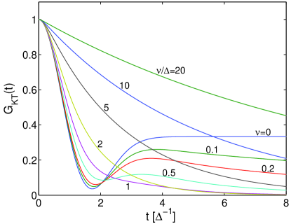
Figure 1: Dynamic Kubo-Toyabe function calculated by Eq. (23) on $N=8192$ sampling points for several scattering frequencies $\nu$.

In order to benchmark the computational efficiency of the DTSCM-based method, we calculated the dynamical Kubo-Toyabe function for the same $\nu/\Delta$ values as in figure 3(a) of Hayano et al.Hayano et al. (1979) on several personal computers. The $G_{\rm KT}(t)$ curves, calculated on an array of $N=8192$ sampling points (the typical histograms length e.g. of the datasets from the Paul Scherrer Institute muon facility), are plotted in Fig. 1. The calculation in Matlab took a $0.4$ s overall CPU time on an AMD Athlon processor at 750 MHz dating back to year 2000, and approximately one tenth on a recent PC (Pentium G2030 CPU at 3.0 GHz). A fit of real $\mu$SR data, requiring typically several hundreds function calls, can be therefore performed by means of Eq. (23) virtually in real time even on a very low-end computer.

The accuracy of the discrete-time approximation with a reasonable sampling interval, possibly identical to the native experimental resolution in the time-differential data, is another issue of our method. To this end, we tested the DTSCM solution against analytical or approximate solutions of the continuous-time SCM in two cases. The first benchmark is provided by the SCM in the presence of a Lorentzian field distribution, whose exact solution is given by Eq. (9). The polarization function $G_{\rm L}(T)$ is plotted in Fig. 2 for several values of the scattering frequency $\nu$. The discrete-time ($N=512$) and continuous-time solutions $G_{\rm L}^{\rm DT}$, $G_{\rm L}^{\rm CT}$ are practically overlapped and undistinguished in the plot. In spite of the rather coarse time sampling, their difference $G_{\rm L}^{\rm DT}(t)-G_{\rm L}^{\rm CT}(t)$ (figure inset) is negligible for practical purposes even at comparatively high $\nu$. For reference, the experimental relative uncertainty on the muon polarization in very-high-statistics measurements is seldom smaller than a few permil.

Another well-known case is the Gaussian field distribution in the extreme narrowing limit $\nu\gg\Delta$. Its relaxation function is approximated by the so-called Abragam formula Abragam (1961); Keren (1994); Kehr et al. (1978)

$${}G^{\rm AF}(t)=\exp(-2\Delta^{2}\nu^{-2})\left(\exp(-\nu t)-1+\nu t\right)$$ (24)

which is asymptotically exact for $\nu/\Delta\to\infty$. The accuracy of Eq. (23) in reproducing Eq. (24) is exemplified in Fig. 3, showing simulations obtained by the DTSCM at $\nu=320\Delta$ and different time resolutions. Here again, the difference $G^{\rm DT}(t)-G^{\rm AF}$ between the discrete-time and the continuous-time solution given by the Abragam approximate formula is negligible even with a relatively coarse-grained sampling, corresponding to a cumulative scattering probability over a time bin $1-\exp(-\nu\tau)$ on the order of ten percent.

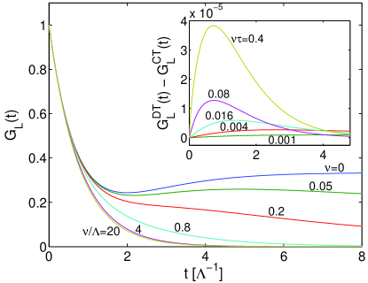
Figure 2: Lorentzian field distribution. Main panel: dynamic polarization function $G_{\rm L}(t)$ for several scattering frequencies $\nu$. Inset: difference between $G_{\rm L}(t)$ calculated by the DTSCM method Eq. (23) over $N=512$ sampling points, and the exact continuous-time solution Eq. (9), for the various $\nu$ values.

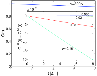
Figure 3: Gaussian field distribution in the extreme narrowing limit ($\nu=320\Delta$). Main panel: dynamic polarization function $G(t)$. Inset: difference between $G(t)$ calculated by the DTSCM-based (DT) method Eq. (23) and the Abragam formula (AF) asymptotic solution Eq. (24), for several sampling intervals $\tau$.

V Conclusions

In conclusion, we have demonstrated an accurate and efficient numerical method to calculate the dynamical Kubo-Toyabe function describing the longitudinal muon polarization function $G(t)$ vs. time in the presence of muon diffusion as well as, in principle, the solution of the SCM for an arbitrary distribution of static internal fields. The error on $G(t)$ produced by time discretization is found to be much smaller than the experimental uncertainty even with very coarse time resolutions, and data oversampling is not needed. If implemented by means of the FFT algorithm, the method requires negligible CPU resources, which makes it suitable to fit experimental data in real time even on a slow computer.

Appendix A Proof that $G^{\prime}$ tends to $G$ for $\alpha\to\infty$

We sketch here the proof that $G^{\prime}$, defined by Eq. (23), is an asymptotically exact solution of Eq. (15) for $\alpha\to\infty$. It is easily shown that the exponentially weighted function $\tilde{G}^{\prime}_{n}$ ($0\leq n<2N$) defined by Eq. (22) obeys the equation

$${}{\tilde{G}^{\prime}}={\tilde{H}}^{(0)}+\frac{\lambda}{q}\,({\tilde{H}}^{(0)}-\delta)\ast{\tilde{G}^{\prime}}$$ (25)

formally identical to Eq. (17) but for the replacement of non-circular with circular convolution. Upon defining ${\tilde{K}}^{(0)}\equiv{\tilde{H}}^{(0)}\!-\delta$, the following series expansion is straightforwardly obtained from Eq. (25):

$${}{\tilde{G}^{\prime}} = {\tilde{H}}^{(0)}+\frac{\lambda}{q}\,{\tilde{K}}^{(0)}\!\ast{\tilde{H}}^{(0)}+\frac{\lambda^{2}}{q^{2}}\,{\tilde{K}}^{(0)}\!\ast{\tilde{K}}^{(0)}\!\ast{\tilde{H}}^{(0)}+$$ (26)

$$\mskip-32.0mu\frac{\lambda^{3}}{q^{3}}\,{\tilde{K}}^{(0)}\!\ast{\tilde{K}}^{(0)}\!\ast{\tilde{K}}^{(0)}\!\ast{\tilde{H}}^{(0)}+\dots$$

$$\equiv \sum_{m=0}^{\infty}{\tilde{\cal A}}^{(m)}$$

to be compared with the analogous expansion for the exact solution ${\tilde{G}}_{n}$ ($0\leq n<N$) drawn from Eq. (17),

$${}{\tilde{G}} = {\tilde{H}}^{(0)}+\frac{\lambda}{q}\,\mbox{\rm conv}\!\left({\tilde{K}}^{(0)},{\tilde{H}}^{(0)}\right)+$$ (27)

$$\mskip-32.0mu\frac{\lambda^{2}}{q^{2}}\,\mbox{\rm conv}\!\left({\tilde{K}}^{(0)},\,\mbox{\rm conv}\!\left({\tilde{K}}^{(0)},{\tilde{H}}^{(0)}\right)\right)+$$

$$\mskip-32.0mu\frac{\lambda^{3}}{q^{3}}\,\mbox{\rm conv}\!\left({\tilde{K}}^{(0)},\,\mbox{\rm conv}\!\left({\tilde{K}}^{(0)},\,\mbox{\rm conv}\!\left({\tilde{K}}^{(0)},{\tilde{H}}^{(0)}\right)\right)\right)+\dots$$

$$\equiv \sum_{m=0}^{\infty}{\tilde{\cal C}}^{(m)}$$

which is actually a finite summation, as ${\tilde{\cal C}}^{(m)}$ vanish identically for $m>N$ (see Eq. (III)).

The series Eq. (26) is absolutely convergent for any positive $\alpha$. Its $m$-th term ${\tilde{\cal A}}^{(m)}$ clearly obeys the recursion relation

$${}{\tilde{\cal A}}^{(m+1)}=\frac{\lambda}{q}\,{\tilde{K}}^{(0)}\!\ast{\tilde{\cal A}}^{(m)}.$$ (28)

Taking into account that $\left|{{\tilde{K}_{n}}^{(0)}}\right|\leq\exp(-(\alpha+\nu\tau)n)$, from Eq. (28) we can set the following upper bound:

$${}\left|{{\tilde{\cal A}_{n}}^{(m+1)}}\right| \leq \frac{\lambda}{q}\sum_{k=1}^{N-1}{\rm e}^{-(\alpha+\nu\tau)n}\max{{\tilde{\cal A}}^{(m)}}$$ (29)

$$\mskip-76.0mu={\rm e}^{-\alpha}\left(1-{\rm e}^{-(\alpha+\nu\tau)(N-1)}\right)\frac{1-{\rm e}^{-\nu\tau}}{1-{\rm e}^{-(\alpha+\nu\tau)}}\max{{\tilde{\cal A}}^{(m)}}$$

$$\mskip-76.0mu<{\rm e}^{-\alpha}\max{{\tilde{\cal A}}^{(m)}}$$

whence, by induction, $\left|{{\tilde{\cal A}_{n}}^{(m)}}\right|<A\exp({-\alpha m})$ with $A$ being a suitable positive constant. This ensures the absolute convergence of the series.

We now evaluate the difference ${\tilde{E}}_{n}\equiv{\tilde{G}}^{\prime}_{n}-{\tilde{G}}_{n}$ ($0\leq n<N$) term by term from Eq. (26) and Eq. (27):

$${}{\tilde{E}}_{n}=\sum_{m=2}^{\infty}{\tilde{\cal E}}_{n}^{(m)}=\sum_{m=2}^{\infty}{\tilde{\cal A}}_{n}^{(m)}-{\tilde{\cal C}}_{n}^{(m)}$$ (30)

where the first non-zero term in the sum is $m=2$, since ${\tilde{\cal A}}_{n}^{(1)}={\tilde{\cal C}}_{n}^{(1)}$ owing to Eq. (19). The $m$-th term ${\tilde{\cal A}}_{n}^{(m)}$ in Eq. (26) is expressed as

$${}{\tilde{\cal A}}_{n}^{(m)}=\frac{\lambda^{m}}{q^{m}}\underbrace{\sum_{k=0}^{N-1}\dots\sum_{s=0}^{N-1}}_{m\ {\rm times}}{\tilde{K}}^{(0)}_{k}\dots\tilde{K}^{(0)}_{s}{\tilde{H}}_{{\rm mod}(n-k\,\dots-s,2N)}^{(0)}$$ (31)

where the summation indices are upper-limited to $N-1$ since ${\tilde{K}}^{(0)}$ is a zero-padded vector. On the other hand, ${\tilde{\cal C}}_{n}^{(m)}$ from Eq. (27) is calculated as

$${}{\tilde{\cal C}}_{n}^{(m)}=\frac{\lambda^{m}}{q^{m}}\underbrace{\sum_{k=0}^{N-1}\dots\sum_{s=0}^{N-1}}_{m\ {\rm times}}{\tilde{K}}^{(0)}_{k}\dots\tilde{K}^{(0)}_{s}{\tilde{H}}_{n-k\,\dots-s}^{(0)}$$ (32)

where it is intended that ${\tilde{H}}_{j}^{(0)}=0$ for $j<0$. Equations (31) and (32) may also be written as

$${}{\tilde{\cal A}}_{n}^{(m)}\! = \frac{\lambda^{m}}{q^{m}}\overbrace{\sum_{k=0}^{N-1}\dots\sum_{s=0}^{N-1}}^{m\ {\rm times}}\sum_{t=0}^{N-1}{\tilde{K}}^{(0)}_{k}\dots\tilde{K}^{(0)}_{s}{\tilde{H}}_{t}^{(0)}\times$$

$$\mskip-40.0mu\left(\delta_{n-k\,\dots-s,t}+\delta_{2N+n-k\,\dots-s,t}+\delta_{4N+n-k\,\dots-s,t}+\dots\right)$$

and

$${}{\tilde{\cal C}}_{n}^{(m)}=\frac{\lambda^{m}}{q^{m}}\underbrace{\sum_{k=0}^{N-1}\dots\sum_{s=0}^{N-1}}_{m\ {\rm times}}\sum_{t=0}^{N-1}{\tilde{K}}^{(0)}_{k}\dots\tilde{K}^{(0)}_{s}{\tilde{H}}_{t}^{(0)}\delta_{n-k\,\dots-s,t}$$ (34)

respectively, whence ${\tilde{\cal E}}_{n}^{(m)}$ is expressed as

$${}{\tilde{\cal E}}_{n}^{(m)}=\frac{\lambda^{m}}{q^{m}}\overbrace{\sum_{k=0}^{N-1}\dots\sum_{s=0}^{N-1}}^{m\ {\rm times}}\sum_{t=0}^{N-1}{\tilde{K}}^{(0)}_{k}\dots\tilde{K}^{(0)}_{s}{\tilde{H}}_{t}^{(0)}\left(\delta_{2N+n-k\,\dots-s,t}+\delta_{4N+n-k\,\dots-s,t}+\dots\right).$$ (35)

The latter expression is subject to the following bound:

$${}\left|{{\tilde{\cal E}}_{n}^{(m)}}\right| \leq \frac{\lambda^{m}}{q^{m}}\overbrace{\sum_{k=0}^{N-1}\dots\sum_{s=0}^{N-1}}^{m\ {\rm times}}\sum_{t=0}^{N-1}{\rm e}^{-k(\alpha+\nu\tau)}\dots\rm e^{-s(\alpha+\nu\tau)}{\rm e}^{-t(\alpha+\nu\tau)}\left(\delta_{2N+n-k\,\dots-s,t}+\delta_{4N+n-k\,\dots-s,t}+\dots\right)$$

$$= \frac{\lambda^{m}}{q^{m}}\,{\rm e}^{-n(\alpha+\nu\tau)}\!\sum_{k=0}^{N-1}\dots\sum_{s=0}^{N-1}\sum_{t=0}^{N-1}\left(\delta_{2N+n-k\,\dots-s,t}\,{\rm e}^{-2N(\alpha+\nu\tau)}+\delta_{4N+n-k\,\dots-s,t}\,{\rm e}^{-4N(\alpha+\nu\tau)}+\dots\right)$$ (36)

$$= \frac{\lambda^{m}}{q^{m}}\,{\rm e}^{-(n+2N)(\alpha+\nu\tau)}\!\sum_{h=1}^{m/2}{\cal N}(m,n+2hN)\,{\rm e}^{-2(h-1)N(\alpha+\nu\tau)}$$

where ${\cal N}(m,n)$ denotes the number of combinations whereby the sum of $m+1$ integer addends each in the range $[0,N-1]$ may yield $n$. It follows that the unweighted difference $E_{n}=G^{\prime}_{n}-G_{n}={\tilde{E}}_{n}\exp(\alpha n)$ is bounded as

$${}\left|{E_{n}}\right| \leq {\rm e}^{-2N\alpha}\,{\rm e}^{-(n+2N)\nu\tau}\sum_{m=2}^{\infty}\frac{\lambda^{m}}{q^{m}}\times\phantom{\mskip 120.0mu~{}}$$ (37)

$$\left[\sum_{h=1}^{m/2}{\cal N}(m,n+2hN)\,{\rm e}^{-2(h-1)N(\alpha+\nu\tau)}\right]$$

where the expression on the right hand side tends to zero for $\alpha\to\infty$, since the series (which is convergent in view of Eq. (29)) is a decreasing function of $\alpha$, while its prefactor vanishes. Therefore $\lim_{\alpha\to\infty}E_{n}=0$.