Cost minimization for fading channels with energy harvesting and conventional energy

Abstract

In this paper, we investigate resource allocation strategies for a point-to-point wireless communications system with hybrid energy sources consisting of an energy harvester and a conventional energy source. In particular, as an incentive to promote the use of renewable energy, we assume that the renewable energy has a lower cost than the conventional energy. Then, by assuming that the non-causal information of the energy arrivals and the channel power gains are available, we minimize the total energy cost of such a system over $N$ fading slots under a proposed outage constraint together with the energy harvesting constraints. The outage constraint requires a minimum fixed number of slots to be reliably decoded, and thus leads to a mixed-integer programming formulation for the optimization problem. This constraint is useful, for example, if an outer code is used to recover all the data bits. Optimal linear time algorithms are obtained for two extreme cases, i.e., the number of outage slot is $1$ or $N-1$. For the general case, a lower bound based on the linear programming relaxation, and two suboptimal algorithms are proposed. It is shown that the proposed suboptimal algorithms exhibit only a small gap from the lower bound. We then extend the proposed algorithms to the multi-cycle scenario in which the outage constraint is imposed for each cycle separately. Finally, we investigate the resource allocation strategies when only causal information on the energy arrivals and only channel statistics is available. It is shown that the greedy energy allocation is optimal for this scenario.

I Introduction

Driven by environmental concerns, green wireless communications have recently attracted increasing attention from both industry and academia. It is reported in [1] that the world-wide cellular networks consume about sixty billion kilowatt hour (kWh) of energy per year, which result in a few hundred million tons of carbon dioxide emission yearly. These figures are expected to increase rapidly in the near future if no further actions are taken. On the other hand, it is pointed out in [2] that, with the explosive growth of high data rate wireless applications, more energy is consumed to guarantee the users’ quality of service (QoS). These facts create a compelling need for green wireless communications. One way to achieve green wireless communications is to improve the energy-efficiency of the current communications networks [3]. Another way is to introduce clean and environment-friendly renewable energy (such as solar power and wind power) to wireless communications networks [4].

Introducing energy harvesting capabilities to wireless communications is a promising approach to achieve green communications, with its great potential to reduce the carbon dioxide emission produced by conventional energy. However, it poses lots of new challenges on the design of resource allocation strategies for the wireless communications networks. This is mainly due to the highly time-varying availability of the renewable energy. For instance, solar energy and wind energy may vary significantly over time and locations depending on the weather and the climate conditions. Thus, conventional transmit power constraints are not suitable to model communications devices with renewable energy. Instead, resource has to be allocated subject to energy harvesting constraints. With energy harvesting constraints, in every time slot, the transmitter is allowed to use at most the amount of harvested and stored energy currently available. In other words, the transmitter can not consume any energy harvested in future.

Throughput optimization for wireless communications systems with such energy harvesting constraints has been extensively studied in recent literatures. The capacity of AWGN channel with the energy harvesting system setup was studied in [5] and [6]. Throughput maximization for a single-user energy harvesting system with a deadline constraint in a static channel was studied in [7] and [8]. For single-user fading channel, the optimal energy allocation scheme to maximize the throughput for a slotted system over a finite horizon of time slots was obtained in [9] through dynamic programming. In [10], the authors derived continuous time optimal policies to maximize the throughput of fading channels with the energy harvesting constraints. Then, energy allocation strategies to maximize the throughout of multiple access channels and broadcast channels with energy harvesting constraints were investigated in [11] and [12]. Throughput maximization for relay channels with energy harvesting constraints was studied in [13].

Another line of related research in wireless communications with energy harvesting nodes focused on simultaneous wireless information and power transfer [14, 15, 16, 17, 18, 19, 20]. The idea of simultaneous wireless information and power transfer was proposed in [14]. In [15], the authors studied the tradeoff between information rate and power transfer in a frequency selective wireless system. Then, the tradeoff between energy and information for a MIMO broadcast system was studied in [16]. In [17, 18], operation protocols and switching schemes to minimize the outage probability for wireless systems with simultaneous information and power transfer were studied. In [19], practical receiver designs for implementing simultaneous information and power transfer were investigated. In [20], a new protocol was proposed to achieve simultaneous bi-directional wireless information and power for a multi-user communication network.

In these aforementioned works, the communications devices are powered only by the renewable energy. However, due to the highly random availability of the renewable energy, communications devices powered only by the renewable energy may not be able to guarantee a required level of QoS. Since in many communication systems, such as in a cellular communications, the QoS must be satisfied at least with high probability, a hybrid energy supply system with both renewable energy supply and conventional energy supply is preferred in practice. This motivated us to consider a communications system with both energy harvesters and conventional energy supply in this paper. As an incentive to promote the use of the renewable energy, we assume that the renewable energy has a lower cost than the conventional energy. Under this assumption, minimizing the energy consumption is not equivalent to minimizing the energy cost. In this paper, unlike the conventional energy-efficient studies whose objective is minimizing the energy consumption, our objective is to minimize the total energy cost. The motivation for this is that, from a user’s perspective, minimizing the total energy cost is more important and meaningful. It is worth pointing out that hybrid energy supply model was also considered in [21, 22, 23, 24]. However, the focus of [21] was to develop the energy cooperation scheme between two cellular base stations. The target of [22] is to derive the resource allocation scheme to maximize the weighted energy efficiency of data transmission over a downlink orthogonal frequency division multiple access (OFDMA) system. The objective of [23] and [24] were to maximize the throughput and minimize the energy consumption for a point-to-point channel, respectively.

The contribution and the main results of this paper are summarized as follows.

• We consider a point-to-point communications system with both renewable energy and conventional energy. To guarantee the QoS of the system, we propose an outage constraint, which requires a minimum number of slots to be reliably decoded. This constraint is useful if, for example, an outer code is used to recover all data bits. A mixed integer programming problem is then formulated to minimize the total energy cost of such a system for $N$ fading slots under both energy harvesting constraints and the proposed outage constraint.

• We study the optimal power allocation strategy to minimize the total energy cost by assuming full knowledge of the channel and energy state information (CESI). By exploring the structured properties of the optimal solution, we propose two low complexity algorithms with worst case linear time complexity to yield the optimal power allocation for two extreme cases: when the number of outage slot is either $1$ or $N-1$.

• For the general case, we propose a lower bound based on linear programming relaxation. Besides, we propose two suboptimal algorithms referred to as linear programming based channel removal (LPCR) and worst channel removal (WCR), respectively. It is shown by simulation that the proposed suboptimal algorithms exhibit only a small gap with respect to the lower bound. It is proved that WCR is optimal when certain conditions are satisfied.

• We extend the proposed algorithms and the obtained results to the multi-cycle scenario where the outage constraint is imposed for each cycle separately. It is shown that the proposed algorithms can be easily extended to the multi-cycle scenario with few modifications.

• When CESI is not available, a new outage constraint is proposed. Closed-form solution is obtained for this case. It is shown that the optimal solution has a greedy feature. It always uses the low-cost energy first and uses the high-cost energy only when necessary (i.e., when the low-cost energy is not enough to guarantee the required QoS).

The rest of this paper is organized as follows. We describe the system model in Section II and give out the problem formulation in Section III. The proposed algorithms and obtained theoretical results are then presented in Section IV. In Section V, we investigate the power allocation strategy when future CSI and energy harvesting information is not available. Then, in Section VI, numerical results are presented to verify the proposed studies. Finally, Section VII concludes the paper.

II System Model

In this paper, we consider a point-to-point channel with one transmitter (Tx) and one receiver (Rx). We assume that the transmitter has access to two types of energy: conventional energy and renewable energy. The conventional energy is obtained from conventional power grid or batteries. The renewable energy is obtained by energy harvesting devices, such as solar panel and wind turbine. These two types of energy are provided to the transmitter at different prices: $\alpha$ per unit for conventional energy, and $\beta$ per unit for renewable energy. For exposure, we make the following assumptions in this paper.

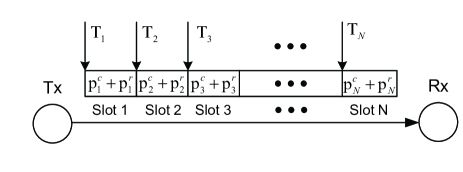
Figure 1: System Model

• $\alpha>\beta$. We make this assumption due to the following two reasons: (i) The renewable energy greatly depends on the environment (such as the weather), and thus is not as reliable as the conventional energy. Therefore, the renewable energy should be priced lower to attract users. (ii) The renewable energy is clean and environment-friendly. Thus, pricing the renewable energy at a lower price provides an incentive for users to use green energy.

• The transmission is slotted, and the Tx is equipped with an energy storage device. The energy harvested at the beginning of slot $i$ is denoted by $T_{i}$. Thus, the harvested energy $T_{i}$ can be used is slot $i$ or stored for future use. The conventional energy and the renewable energy consumed at slot $i$ are denoted as $p_{i}^{c}$ and $p_{i}^{r}$, respectively.

• The channel experiences block-fading and remains constant during each transmission slot, but possibly changes from one slot to another. The channel power gain is assumed to be a random variable with a continuous probability density function (PDF) $f(x)>0,\forall x>0$. The channel power gain for slot $i$ is denoted as $g_{i}$. The noise at the Rx is assumed to be a circular symmetric complex Gaussian random variable with zero mean and variance $N_{0}$ denoted by $\mathcal{CN}(0,N_{0})$.

III Problem Formulation

In this paper, we assume that the whole transmission process consists of $N$ time slots. Under the system model given in Section II, the instantaneous transmission rate in slot $i$ can be written as $\ln(1+\frac{g_{i}\left(p_{i}^{c}+p_{i}^{r}\right)}{N_{0}})$. Thus, if the target transmission rate of the user is $R$, the minimum power required to support this rate is

$$p_{i}^{inv}=\frac{N_{0}~{}\left(e^{R}-~{}1\right)}{g_{i}}.$$ (1)

We refer to $p_{i}^{inv}$ as channel inversion power for slot $i$. If $p_{i}^{c}+p_{i}^{r}<p_{i}^{inv}$, we say the user is in outage in slot $i$. For convenience, we define an indicator function for each slot, which is given as

$$\chi_{i}\left(p_{i}^{c},p_{i}^{r}\right)=\left\{\begin{array}[]{ll}1,&~{}\mbox{if}~{}\ln\left(1+\frac{g_{i}\left(p_{i}^{c}+p_{i}^{r}\right)}{N_{0}}\right)<R,\\ 0,&~{}\mbox{otherwise}.\end{array}\right.$$ (4)

To guarantee the QoS, we assume that the fraction of outage should be kept below a prescribed target $\epsilon$. Mathematically, this can be written as

$$\frac{1}{N}\sum_{i=1}^{N}\chi_{i}\left(p_{i}^{c},p_{i}^{r}\right)\leq\epsilon,$$ (5)

where $\chi_{i}\left(p_{i}^{c},p_{i}^{r}\right)$ is given by (4). In this paper, we refer to this constraint as outage constraint. This outage constraint requires at least $\lceil N(1-\epsilon)\rceil$ packets to be received without error over $N$ slots, which is useful for delay-sensitive data or when an outer code is used that can correct any $\lfloor N(1-\epsilon)\rfloor$ packets in outage. Clearly, if $\epsilon=0$, no outage is allowed.

In this paper, we assume that the harvested energy can be stored for future use. Thus, the energy harvesting constraints can be written as

$$\sum_{i=1}^{k}p_{i}^{r}-\sum_{i=1}^{k}T_{i}\leq 0,\forall k\in\left\{1,2,\cdots,N\right\}.$$ (6)

In this paper, our objective is to minimize the total energy cost of the $N$-slot transmission through proper energy allocation strategies. Under the constraints described above, the problem can be formulated as follows.

Problem 1

$$\min_{p_{i}^{c},~{}p_{i}^{r}} \sum_{i=1}^{N}\left(\alpha p_{i}^{c}+\beta p_{i}^{r}\right),$$ (7)

s.t. $$~{}p_{i}^{c}\geq 0,~{}p_{i}^{r}\geq 0,\forall i\in\left\{1,2,\cdots,N\right\},$$ (8)

$$\sum_{i=1}^{k}p_{i}^{r}-\sum_{i=1}^{k}T_{i}\leq 0,\forall k\in\left\{1,2,\cdots,N\right\},$$ (9)

$$\frac{1}{N}\sum_{i=1}^{N}\chi_{i}\left(p_{i}^{c},p_{i}^{r}\right)\leq\epsilon,$$ (10)

where $\chi_{i}\left(p_{i}^{c},p_{i}^{r}\right)$ is given by (4). For notation convenience, we use $\chi_{i}$ instead of $\chi_{i}\left(p_{i}^{c},p_{i}^{r}\right)$ in the rest of the paper. Problem 1 is a mixed integer optimization problem, which is difficult to solve optimally [25].

For the problem considered here, we assume full CESI, i.e., the channel power gains (i.e., $[g_{1},g_{2},\cdots,g_{N}]^{T}$) and the energy harvesting state information (i.e., $[T_{1},T_{2},$ $\cdots,T_{N}]^{T}$) are known at the Tx as a priori. This assumption is fairly strong and may not be practical. However, the solution provides a lower bound on the energy cost and sheds insights on the design of energy allocation strategies with partial CESI where not all information is available in advance.

IV Theoretical Results

We start by analyzing this problem to obtain structural properties of the optimal solution, which is useful in developing good sub-optimal algorithms later.

IV-A Properties of Problem 1

Proposition 1

Denote the set of slots in which the user is in outage as $\mathcal{S}$. Then, at the optimal solution of Problem 1, we have $|\mathcal{S}^{*}|=\lfloor N\epsilon\rfloor$, where $|\cdot|$ denotes the cardinality of a set and $\lfloor x\rfloor$ denotes the largest integer not greater than $x$.

Proof:

First, any feasible solution of Problem 1 must satisfy the constraint (10). Thus, we have $|\mathcal{S}^{*}|\leq\lfloor N\epsilon\rfloor$. Now, suppose $|\mathcal{S}^{*}|<\lfloor N\epsilon\rfloor$. Then, we can always drop more slots such that (10) holds with equality. Thus, the energy cost of these slots becomes zero. Obviously, by doing this, the value of (7) is reduced. This contradicts with our presumption that $|\mathcal{S}^{*}|<\lfloor N\epsilon\rfloor$. Thus, $|\mathcal{S}^{*}|$ must be equal to $\lfloor N\epsilon\rfloor$. ∎

Proposition 1 indicates that the optimal allocation strategy is to drop as many slots as allowed by the outage constraint. In those dropped slots, the user should shut down its transmission, and thus consumes no energy.

We next consider the case where the set of outage slots is fixed, and determine the optimal power allocation policy under this condition. We first state a Lemma that may be of independent technical interest.

Lemma 1

An optimal policy for the following linear program

$$\min_{x_{i}}~{} \alpha\sum_{i=1}^{N}c_{i}-(\alpha-\beta)\sum_{i=1}^{N}x_{i},$$ (11)

s.t. $$~{}0\leq x_{i}\leq c_{i},\forall i\in\{1,2,\ldots,N\},$$ (12)

$$\sum_{i=1}^{k}x_{i}-\sum_{i=1}^{k}T_{i}\leq 0,\forall k\in\left\{1,2,\cdots,N\right\}.$$ (13)

is given by $x_{i}^{*}=\min\{c_{i},\sum_{j=1}^{i}T_{j}-\sum_{j=1}^{i-1}x^{*}_{j}\}$ for $i\in\{1,2,\ldots,N\}$.

Proof of this lemma follows from observing that the policy satisfies the Karush-Kuhn-Tucker (KKT) conditions [26] for the linear program. Since the KKT conditions are sufficient for optimality of linear programs [26], this policy is optimal. The proof is given in the Part A of the Appendix.

Proposition 2

For any given set $\mathcal{S}$, the power allocation strategy $\boldsymbol{p}_{k}^{*}=[p_{k}^{r},~{}p_{k}^{c}]^{T}$ given below is optimal.

$$\boldsymbol{p}_{k}^{*}=\left\{\begin{array}[]{ll}\hat{\boldsymbol{p}}_{k}^{*},&~{}\forall k\in\mathcal{S},\\ \tilde{\boldsymbol{p}}_{k}^{*},&~{}\forall k\in\mathcal{S}^{c},\end{array}\right.$$ (16)

where $\hat{\boldsymbol{p}}_{k}^{*}=[0,~{}0]^{T}$, $\tilde{\boldsymbol{p}}_{k}^{*}=\left[p_{k}^{r*},p_{i}^{inv}-p_{k}^{r*}\right]^{T}$ with $p_{k}^{r*}=\min\left\{p_{i}^{inv},\sum_{i=1}^{k}T_{i}-\sum_{i=1}^{k-1}p_{i}^{r}\right\}$, and $\mathcal{S}^{c}$ denotes the complement of $\mathcal{S}$.

Proof:

It is observed that if $\mathcal{S}$ is given, Problem 1 can be converted to

Problem 2

$$\min_{p_{i}^{c},~{}p_{i}^{r}} \left(\alpha\sum_{i\in\mathcal{S}^{c}}p_{i}^{c}+\beta\sum_{i\in\mathcal{S}^{c}}p_{i}^{r}\right),$$ (17)

s.t. $$~{}p_{i}^{c}\geq 0,~{}p_{i}^{r}\geq 0,~{}i\in\mathcal{S}^{c},$$ (18)

$$\sum_{i=1}^{k}p_{i}^{r}-\sum_{i=1}^{k}T_{i}\leq 0,\forall k\in\left\{1,2,\cdots,N\right\},$$ (19)

$$\ln(1+\frac{g_{i}\left(p_{i}^{c}+p_{i}^{r}\right)}{N_{0}})\geq R,\forall i\in\mathcal{S}^{c},$$ (20)

where $\mathcal{S}^{c}$ denotes the complement of $\mathcal{S}$.

It is not difficult to observe that (20) is equivalent to $p_{i}^{c}+p_{i}^{r}\geq p_{i}^{inv},\forall i\in\mathcal{S}^{c}.$ Obviously, the objective function is minimized when it holds with equality for all $i\in\mathcal{S}^{c}$, i.e., $p_{i}^{c}+p_{i}^{r}=p_{i}^{inv},\forall i\in\mathcal{S}^{c}.$ Furthermore, it is also easy to see that our optimization problem is equivalent to setting $p^{inv}_{i}=0$ for all $i\in\mathcal{S}$. Based on these observations, Problem 2 can be converted to

Problem 3

$$\min_{p_{i}^{r}}~{} \alpha\sum_{i\in\mathcal{S}^{c}}p_{i}^{inv}-(\alpha-\beta)\sum_{i\in\mathcal{S}^{c}}p_{i}^{r},$$ (21)

s.t. $$~{}0\leq p_{i}^{r}\leq p_{i}^{inv},\forall i\in\mathcal{S}^{c},$$ (22)

$$\sum_{i=1}^{k}p_{i}^{r}-\sum_{i=1}^{k}T_{i}\leq 0,\forall k\in\left\{1,2,\cdots,N\right\}.$$ (23)

We note that Problem 3 has the same structure as the linear program in Lemma 1. Applying Lemma 1 to with $c_{i}=p_{i}^{inv}$ and $x_{i}=p_{i}^{r}$ then concludes our proof of Proposition 2. ∎

Proposition 2 indicates that the power allocation is zero for both conventional and harvested energy in dropped slots. This is clearly optimal in terms of energy saving. It is also observed that for the remaining slots, the harvested energy should be used first. If the harvested energy is not enough to support the target rate during these slots, conventional energy should be used as a compensation. This is similar to the greedy use of harvested energy whenever possible, and thus highlights the fundamental difference of prioritizing the use of (cheap) harvested energy over (expensive) conventional energy. Thus, for convenience, we refer to the power allocation given in (16) as Greedy Power Allocation.

IV-B Optimal Power Allocation Algorithms

From the results obtained in Proposition 1 and Proposition 2, it is observed that Problem 1 in general can be solved in two steps: (1) Find the set of the time slots that should be dropped, i.e., $\mathcal{S}$. (2) Apply the greedy power allocation given in (16) for the time slots in $\mathcal{S}^{c}$. The difficulty of Problem 1 lies primarily in the first step, i.e., find the optimal $\mathcal{S}^{*}$ and its complement $(\mathcal{S}^{*})^{c}$. We start our analysis from two extreme cases ($\lfloor N\epsilon\rfloor=1$ and $\lfloor N\epsilon\rfloor=N-1$) and then extend the results to the general case ($\lfloor N\epsilon\rfloor=M$).

1) $\lfloor N\epsilon\rfloor=1$: This case is to drop one slot.

Theorem 1

When $\lfloor N\epsilon\rfloor=1$, for any slot $i\in\{1,2,\cdots,N\}$, if there is a slot before slot $i$ requiring more channel inversion power than slot $i$, then slot $i$ should be kept, i.e, $i\in(S^{*})^{c}$.

Proof:

Suppose that there is a slot $k$, where $k<i$, and $p_{k}^{inv}>p_{i}^{inv}$. Now, we consider the following two scenarios:

Scenario 1: Slot $i$ is dropped. For the convenience of exposition, we denote the total energy available at slots $k$ and $k+1$ are $E_{k}$ and $E_{k+1}$, respectively. Then, the harvested energy consumed during slot $k$ is $p_{k}^{r}=E_{k}-E_{k+1}$. Then, the energy cost generated by this slot is $\alpha p_{k}^{c}+\beta p_{k}^{r}$, which is equivalent to $\alpha p_{k}^{inv}-(\alpha-\beta)(E_{k}-E_{k+1})$.

Scenario 2: Slot $k$ is dropped. Thus, no energy is consumed in slot $k$ and $p_{k}^{inv}$ in case 1 can be saved for future use. If $E_{k}-E_{k+1}\geq p_{i}^{inv}$, the energy cost generated by slot $i$ is $\beta p_{i}^{inv}$, which is less than $\alpha p_{k}^{c}+\beta p_{k}^{r}$. If $E_{k}-E_{k+1}<p_{i}^{inv}$, the energy cost generated by slot $i$ is $\alpha p_{i}^{inv}-(\alpha-\beta)p_{i}^{r}$. In this case, we let $p_{i}^{r}=E_{k}-E_{k+1}$. It follows that $\alpha p_{i}^{inv}-(\alpha-\beta)(E_{k}-E_{k+1})<\alpha p_{k}^{inv}-(\alpha-\beta)(E_{k}-E_{k+1})$.

It is observed that the energy cost incurred by slot $i$ is always no more than that incurred by slot $k$. Besides, in other time slots, for scenario 2, we can always adopt the power allocation used in scenario 1. Thus, keeping slot $i$ will never result in a larger total energy cost than keeping slot $k$. Theorem 1 is thus proved. ∎

Based on the result given in Theorem 1, we are able to develop the following algorithm to obtain the optimal power allocation scheme for Problem 1.

Algorithm 1 Optimal power allocation for Problem 1 when $\lfloor N\epsilon\rfloor=1$

1:  Calculate the channel inversion power required for each time slot, i.e., $p_{i}^{inv}=\frac{N_{0}\left(e^{R}-1\right)}{g_{i}},\forall i.$

2:  Initialize $p_{idx}=N$.

3:  Initialize a set $\mathcal{A}=\left\{1,2,\cdots,N\right\}$, and a candidate set $\mathcal{B}=\emptyset$.

4:  while $p_{idx}>1$ do

5:     Find the time slot that requires the largest channel inversion power in $\mathcal{A}$ and set the value of its index to $p_{idx}$.

6:     Put this time slot into the set $\mathcal{B}$.

7:     Remove the slot $p_{idx}$ and all the subsequent slots in $\mathcal{A}$.

8:  end while

9:  For any slot $i\in\mathcal{B}$, except the one with the largest $p_{i}^{inv}$, slot $i$ can be removed from $\mathcal{B}$ if the condition $p_{i}^{inv}<T_{i}$ is satisfied.

10:  Perform exhaustive search over the remaining candidates in $\mathcal{B}$.

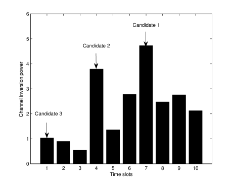
Figure 2: Illustration for Algorithm 1

We give an example to illustrate Algorithm 1 in Fig. 2 with $N=10$. We first put all the $10$ time slots into a set $\mathcal{A}$. It is observed that slot $7$ requires most channel inversion power in $\mathcal{A}$. Thus, we put slot $7$ into the candidate set $\mathcal{B}$ and remove slots $7$ to $10$ from $\mathcal{A}$. It is observed that slot $4$ now requires the largest channel inversion power in $\mathcal{A}$. Therefore, we put slot $4$ into the candidates set $\mathcal{B}$, and remove slots $4$ to $6$ from $\mathcal{A}$. Then, slot $1$ now requires most channel inversion power in $\mathcal{A}$. Thus, we put slot $1$ into the candidates set $\mathcal{B}$ and remove slots $1$ to $3$ from $\mathcal{A}$. Now, in the candidates set $\mathcal{B}$, we have slots $1$, $4$ and $7$. It is clear that only the slot with $T_{i}<p_{i}^{inv}$ may incur an energy cost higher than slot $7$ since it has to use some conventional energy. Thus, for any slot $i$ (except slot $7$) in $\mathcal{B}$ with $T_{i}\geq p_{i}^{inv}$, it can be removed from set $\mathcal{B}$ since it will not incur an energy cost higher than slot $7$. In general, after these procedures, the number of the candidates left in $\mathcal{B}$ is small, and we can easily search for the optimal solution.

2) $\lfloor N\epsilon\rfloor=N-1$: This is equivalent to keeping one slot and dropping $N-1$ slots. By applying the results given in Theorem 1, we are able to develop the following algorithm.

Algorithm 2 Optimal power allocation for Problem 1 when $\lfloor N\epsilon\rfloor=N-1$

1:  Calculate the channel inversion power required for each time slot, i.e., $p_{i}^{inv}=\frac{N_{0}\left(e^{R}-1\right)}{g_{i}},\forall i.$

2:  Initialize $p_{idx}=1$.

3:  Initialize a set $\mathcal{A}=\left\{1,2,\cdots,N\right\}$, and a candidate set $\mathcal{B}=\emptyset$.

4:  while $p_{idx}<N$ do

5:     Find the time slot that requires the smallest channel inversion power in $\mathcal{A}$ and set the value of its index to $p_{idx}$.

6:     Put this time slot into the set $\mathcal{B}$.

7:     Remove all the time slots before $p_{idx}$ (including slot $p_{idx}$) in $\mathcal{A}$.

8:  end while

9:  For any slot $k\in\mathcal{B}$, the slots after slot $k$ can be removed from set $\mathcal{B}$ if $\sum_{i=1}^{k}T_{i}>p_{k}^{inv}$.

10:  Perform exhaustive search over the remaining candidates in $\mathcal{B}$.

We give an example to illustrate Algorithm 2 in Fig. 3. We first put the all $10$ time slots into a set $\mathcal{A}$. It is observed that slot $3$ requires smallest channel inversion power in $\mathcal{A}$. Thus, we put slot $3$ into the candidates set $\mathcal{B}$ and remove slots $1$ to $3$ from $\mathcal{A}$. It is observed that slot $5$ now requires smallest channel inversion power in $\mathcal{A}$. Therefore, we put slot $5$ into the candidates set $\mathcal{B}$ and remove slots $4$ to $5$ from $\mathcal{A}$. Then, slot $10$ now requires smallest channel inversion power in $\mathcal{A}$. Thus, we put slot $10$ into the candidates set $\mathcal{B}$ and remove slots $6$ to $10$ from $\mathcal{A}$. Now, in the candidates set $\mathcal{B}$, we have slots $3$, $5$ and $10$. Then, it is clear that if $\sum_{i=1}^{k}T_{i}>p_{k}^{inv}$, $\forall k\in\mathcal{B}$, the slots after slot $k$ can be removed from set $\mathcal{B}$ due to the fact that slot $k$ will not incur an energy cost higher than those slots after it. In general, after these procedures, the number of the candidates left in $\mathcal{B}$ is quite small, and we can easily search for the optimal solution.

Figure 3: Illustration for Algorithm 2

3) $\lfloor N\epsilon\rfloor=M$: This case is to drop $M$ slots.

Theorem 2

When $\lfloor N\epsilon\rfloor=M$, for any slot $i\in\{1,2,\cdots,N\}$, if there are $M$ slots before slot $i$ requiring more channel inversion power than that of slot $i$, then slot $i$ should not be dropped, i.e, $i\in S^{c}$.

Proof:

Consider the scenario that there are $M$ slots ahead of slot $i$ requiring more channel inversion power than that of slot $i$. Now, we suppose that it is optimal to drop slot $i$. Under these assumptions, there are two possible cases:

• Case 1: All of those $M$ slots are dropped. This implies a total $M+1$ slots are dropped, which contradicts with the fact that $\lfloor N\epsilon\rfloor=M$. Thus, this case cannot happen.

• Case 2: $M-1$ or less lots of those $M$ slots are dropped. For this case, there must exist at least one slot $j$ requiring more channel inversion power than slot $i$ is not dropped. Then, according to Theorem 1, by dropping slot $j$ and keeping slot $i$ instead, we can achieve lower energy cost. This contradicts with our presumption that it is optimal to drop slot $i$.

Combining the above results, it is clear that our presumption does not hold. By contradiction, slot $i$ should be kept for the scenario considered. Theorem 2 is thus proved. ∎

By applying Theorem 2, we can reduce the number of channels under consideration and search over the remaining candidates set.

The proposed optimal power allocation algorithms in this section can greatly reduce the number of candidates when finding the slots to be dropped, especially when $\lfloor N\epsilon\rfloor=1$ and $\lfloor N\epsilon\rfloor=N-1$. However, for the general case $\lfloor N\epsilon\rfloor=M$, the cardinality of the candidates set is still large, and thus the complexity of the optimal power allocation algorithm is quite high. In the following section, we develop two efficient sub-optimal algorithms.

IV-C Suboptimal Power Allocation Algorithms

In this subsection, we propose two suboptimal power allocation schemes for Problem 1, which are given as below.

IV-C1 Linear Programming based Channel Removal (LPCR)

To develop the first algorithm, we consider the following problem

Problem 4

$$\min_{p_{i}^{c},~{}p_{i}^{r},~{}\chi_{i}} \sum_{i=1}^{N}\left(\alpha p_{i}^{c}+\beta p_{i}^{r}\right),$$ (24)

s.t. $$~{}p_{i}^{c}\geq 0,~{}p_{i}^{r}\geq 0,~{}\forall i,$$ (25)

$$\sum_{i=1}^{k}p_{i}^{r}-\sum_{i=1}^{k}T_{i}\leq 0,\forall k\in\left\{1,2,\cdots,N\right\},$$ (26)

$$\sum_{i=1}^{N}\chi_{i}\leq\lfloor N\epsilon\rfloor,$$ (27)

$$p_{i}^{c}+p_{i}^{r}\geq p_{i}^{inv}\left(1-\chi_{i}\right),~{}\forall i,$$ (28)

$$\chi_{i}\in\left\{0,1\right\},~{}\forall i.$$ (29)

Problem 4 is a mixed-integer programming problem, and it is easy to verify that Problem 4 is equivalent to Problem 1. Details are omitted here for brevity.

By taking $\chi_{i}$ as a continuous variable over $[0,1]$ instead of a binary variable, the relaxation problem of Problem 4 is given by

Problem 5

Lower bound of Problem 4

$$\min_{p_{i}^{c},~{}p_{i}^{r},~{}\chi_{i}} \sum_{i=1}^{N}\left(\alpha p_{i}^{c}+\beta p_{i}^{r}\right),$$ (30)

s.t. $$~{}\eqref{Eq-P4-Con1},\eqref{Eq-P4-Con2},\eqref{Eq-P4-Con3},\eqref{Eq-P4-Con4},$$ (31)

$$~{}~{}0\leq\chi_{i}\leq 1,~{}\forall i.$$ (32)

Problem 5 is a linear programming problem, and hence, it can be solved efficiently [27]. It is worth pointing out that Problem 5 provides us a lower bound to Problem 4. Thus, it can be used as a benchmark to investigate the performance of the proposed suboptimal algorithms.

Based on the results of Problem 5, the following suboptimal algorithm for solving Problem 4 is developed.

Algorithm 3 Linear Programming based Channel Removal (LPCR)

1:  Solve Problem 5 by existing linear programming solvers such as CVX [27].

2:  Sort the solution $\left[\chi_{1},\chi_{2},\cdots,\chi_{N}\right]^{T}$ in descending order, and drop the first $\lfloor N\epsilon\rfloor$ slots.

3:  Apply the greedy power allocation scheme given in (16) for the remaining time slots.

The complexity analysis of Algorithm 3 is given as follows. The worst-case complexity of solving the linear program in step $1$ is $O(N^{3})$ (see [25]). The complexity of sorting the obtained solution in descending order in step $2$ is $O(N\log N)$ (see [28]). The complexity of step $3$ is $O(N)$. Thus, the complexity of LPCR is $O(N^{3})$.

IV-C2 Worst-Channel Removal (WCR)

Although the LPCR algorithm has polynomial time complexity, it still requires solving a linear program (Problem 5) with complexity $O(N^{3})$. In this subsection, we propose a simpler suboptimal algorithm, referred to as Worst-Channel Removal (WCR), which has a worst case complexity of $O(N\log N)$.

Algorithm 4 Worst-Channel Removal (WCR)

1:  Sort the time slots according to their channel power gains in the descending order.

2:  Drop the first $\lfloor N\epsilon\rfloor$ slots.

3:  Apply the greedy power allocation scheme given in (16) for the remaining time slots.

The idea of WCR is to remove the worst $\lfloor N\epsilon\rfloor$ channels. It is clear that WCR is in general not optimal. However, when certain conditions are satisfied, WCR is optimal. In the following, we investigate three conditions when WCR is optimal, hence strengthening the motivation of using WCR as a heuristic scheme.

Theorem 3

WCR is the optimal solution of Problem 1 if the condition $\sum_{i=1}^{N}p_{i}^{r}-\sum_{i=1}^{N}T_{i}=0$ is satisfied, i.e., the harvested energy is fully consumed at the end of the transmission.

Proof:

Let $\mathcal{S}$ be the set given in WCR, and we assume that WCR satisfies the condition $\sum_{i=1}^{N}p_{i}^{r}-\sum_{i=1}^{N}T_{i}=0$. Then, according to the proof of Lemma 1, for a given set, Problem 1 can be converted to Problem 3. Thus, under the above assumptions, the value of the objective function under WCR is

$$\alpha\sum_{i\in\mathcal{S}^{c}}p_{i}^{inv}-\left(\alpha-\beta\right)\sum_{i=1}^{N}T_{i}.$$ (33)

Let $\hat{\mathcal{S}}$ be any feasible solution set (other than $\mathcal{S}$) of Problem 1, the value of the objective function under $\hat{\mathcal{S}}$ is then given by

$$\alpha\sum_{i\in\hat{\mathcal{S}}^{c}}p_{i}^{inv}-\left(\alpha-\beta\right)\sum_{i\in\hat{\mathcal{S}}^{c}}p_{i}^{r},$$ (34)

where $\hat{\mathcal{S}}^{c}$ is the complement of $\hat{\mathcal{S}}$. Since $\hat{\mathcal{S}}$ is a feasible solution of Problem 1, it can be observed that $\sum_{i\in\hat{\mathcal{S}}^{c}}p_{i}^{r}\leq\sum_{i=1}^{N}T_{i}$. Since ${\mathcal{S}}$ contains the $\lfloor N\epsilon\rfloor$ time slots with weakest channel power gains, it is easy to verify that $\sum_{i\in\mathcal{S}^{c}}p_{i}^{inv}\leq\sum_{i\in\hat{\mathcal{S}}^{c}}p_{i}^{inv}$. Based on these observations, it is clear that (33) is always lower than (34). Thus, Theorem 3 is proved. ∎

This theorem can be explained in the following way. For any resource allocation schemes that consume all the harvested energy, the cost of the renewable energy for these schemes is the same. Thus, the cost difference among these schemes comes from the cost of the conventional energy. Thus, the scheme consuming less conventional energy has a lower total energy cost. Therefore, it is clear that WCR is optimal when all the harvested energy is consumed.

Theorem 4

WCR is the optimal solution of Problem 1 if no conventional energy is consumed during the whole transmission process.

Proof:

Let $\mathcal{S}$ be the set given in WCR, and it satisfies the condition that no conventional energy is consumed during the whole transmission process. Since no conventional energy is consumed, the value of the objective function of Problem 1 under WCR is given by

$$\sum_{i\in\mathcal{S}^{c}}\beta p_{i}^{r},~{}\mbox{where}~{}p_{i}^{r}=p_{i}^{inv},\forall i\in\mathcal{S}^{c}.$$ (35)

Let $\hat{\mathcal{S}}$ be any feasible solution set (other than $\mathcal{S}$) of Problem 1, the value of the objective function under $\hat{\mathcal{S}}$ is then given by

$$\sum_{i\in\hat{\mathcal{S}}^{c}}\left(\alpha p_{i}^{c}+\beta p_{i}^{r}\right),~{}\mbox{where}~{}p_{i}^{c}+p_{i}^{r}=p_{i}^{inv},\forall i\in\hat{\mathcal{S}}^{c}.$$ (36)

From the fact that $\alpha>\beta$, it follows that $\sum_{i\in\hat{\mathcal{S}}^{c}}\left(\alpha p_{i}^{c}+\beta p_{i}^{r}\right)>\sum_{i\in\hat{\mathcal{S}}^{c}}\beta\left(p_{i}^{c}+p_{i}^{r}\right)$. It is easy to verify that $\sum_{i\in\hat{\mathcal{S}}^{c}}\beta\left(p_{i}^{c}+p_{i}^{r}\right)=\sum_{i\in\hat{\mathcal{S}}^{c}}\beta p_{i}^{inv}>\sum_{i\in\mathcal{S}^{c}}\beta p_{i}^{inv}$ due to the fact that ${\mathcal{S}}$ contains the $\lfloor N\epsilon\rfloor$ time slots with weakest channel power gains. Thus, it is clear that (35) is always less than (36). Theorem 4 is thus proved. ∎

This theorem can be explained in the following way. For any resource allocation schemes that consume no conventional energy, the total energy cost is only determined by the cost of the renewable energy. Thus, the scheme consuming less renewable energy has a lower total energy cost. Therefore, it is clear that WCR is optimal when no conventional energy is consumed.

Theorem 5

For any type of non-decreasing (over time) channel (e.g., AWGN channel), WCR gives the optimal solution of Problem 1.

Proof:

For any type of non-decreasing (over time) channel (e.g., AWGN channel), WCR is equivalent to dropping the first $\lfloor N\epsilon\rfloor$ slots. Let $\mathcal{S}$ be the set that we drop the first $\lfloor N\epsilon\rfloor$ slots, i.e., $\mathcal{S}=\left\{g_{1},g_{2},\cdots,g_{\lfloor N\epsilon\rfloor}\right\}$. To guarantee the QoS of the user during the remaining time slots, the transmit power required is $p_{i}^{c}+p_{i}^{r}=p_{i}^{inv},\forall i\in{\mathcal{S}}^{c}$, where $\mathcal{S}^{c}=\left\{g_{\lfloor N\epsilon\rfloor+1},g_{\lfloor N\epsilon\rfloor+2},\cdots,g_{N}\right\}$.

Now, we consider the set $\hat{\mathcal{S}}=\left\{g_{2},\cdots,g_{\lfloor N\epsilon\rfloor},g_{\lfloor N\epsilon\rfloor+1}\right\}$. To guarantee the QoS of the user during the remaining time slots, the transmit power required is $\hat{p_{i}}^{c}+\hat{p_{i}}^{r}=p_{i}^{inv},\forall i\in\hat{\mathcal{S}}^{c}$, where $\hat{\mathcal{S}}^{c}=\left\{g_{1},g_{\lfloor N\epsilon\rfloor+2},\cdots,g_{N}\right\}$. Since the channel is non-decreasing, it is clear that $g_{1}\leq g_{\lfloor N\epsilon\rfloor+1}$. Thus, it follows $p_{\lfloor N\epsilon\rfloor+1}^{c}+p_{\lfloor N\epsilon\rfloor+1}^{r}\leq\hat{p_{1}}^{c}+\hat{p_{1}}^{r}$. For other time slots, we have $p_{i}^{c}+p_{i}^{r}=\hat{p_{i}}^{c}+\hat{p_{i}}^{r}$. Now, we look at the energy harvest constraints under $\mathcal{S}$ and $\hat{\mathcal{S}}$, respectively. Under $\mathcal{S}$, we have $p_{\lfloor N\epsilon\rfloor+1}^{r}\leq\sum_{i=1}^{\lfloor N\epsilon\rfloor+1}T_{i}$. While under $\hat{\mathcal{S}}$, we have $\hat{p_{1}}^{r}\leq T_{1}$. All the remaining energy harvest constraints are exactly the same for the two cases. Thus, we are always able to set $p_{\lfloor N\epsilon\rfloor+1}^{r}=\hat{p_{1}}^{r}$ and $p_{i}^{r}=\hat{p_{i}}^{r}$ for all the remaining time slots. Then, it is observed that the resultant total energy cost under $\mathcal{S}$ is always less or equal to that under $\hat{\mathcal{S}}$. Using the same approach, we can prove that the total energy cost under $\mathcal{S}$ is lower than that under any other feasible solution set of Problem 1. ∎

This theorem can be explained in the following way. For non-decreasing (over time) channels, the channel inversion power for latter slots is equal to or lower than that for the former slots. Besides, the renewable energy available for the latter slots is in general more than that for the former slots. Thus, dropping the former slots always results in a lower total energy cost. Therefore, it is clear that WCR is optimal for any type of non-decreasing channel.

IV-D The Multi-Cycle Scenario

In the previous subsections, we consider the single-cycle scenario, i.e., the outage constraint is imposed over $N$ continuous slots from one cycle. In this subsection, we consider the multi-cycle scenario, in which the outage constraint is imposed on each cycle. We assume that there are $M$ cycles, and each cycle has $N$ time slots. In each cycle, the maximum number of slots that can be dropped is $K$. Then, the energy cost minimization problem with energy harvesting constraints can be formulated as follows.

Problem 6

$$\min_{p_{i}^{c},~{}p_{i}^{r}} \sum_{i=1}^{MN}\left(\alpha p_{i}^{c}+\beta p_{i}^{r}\right),$$ (37)

s.t. $$~{}p_{i}^{c}\geq 0,~{}p_{i}^{r}\geq 0,~{}\forall i,$$ (38)

$$\sum_{i=1}^{k}p_{i}^{r}-\sum_{i=1}^{k}T_{i}\leq 0,~{}\forall k\in\left\{1,2,\cdots,MN\right\},$$ (39)

$$\sum_{i=(j-1)N+1}^{(j-1)N+N}\chi_{i}\leq K,~{}\forall j\in\left\{1,2,\cdots,M\right\},$$ (40)

where

$$\chi_{i}=\left\{\begin{array}[]{ll}1,&~{}\mbox{if}~{}\ln(1+\frac{g_{i}\left(p_{i}^{c}+p_{i}^{r}\right)}{N_{0}})<R_{i},\\ 0,&~{}\mbox{otherwise}.\end{array}\right..$$ (43)

Since Problem 1 is a special case of Problem 6, we expect the optimal solution of Problem 6 to be hard to obtain. Thus, in this subsection, we develop two suboptimal algorithms to solve Problem 6 based on the LPCR and WCR developed for the one-cycle case. The extension from the one-cycle case to the multi-cycle case depends on an important property of Problem 6, which is presented in the following proposition.

Proposition 3

At the optimal solution of Problem 6, the constraints given by (40) must hold with equality, i.e., $\sum_{i=(j-1)N+1}^{(j-1)N+N}\chi_{i}=K,~{}\forall j\in\left\{1,2,\cdots,M\right\}$.

Proposition 3 can be proved by the same approach as Proposition 1. Thus, details are omitted here for brevity.

In the following, we present the multi-cycle LPCR and the multi-cycle WCR, respectively.

IV-D1 Multi-cycle LPCR

Denote the leftover harvested energy of cycle $i$ as $L_{i}$, and denote the initial storage energy of cycle $i$ as $S_{i}$, we can extend the LPCR to the multi-cycle scenario, which is given as follows.

Algorithm 5 Multi-cycle LPCR

1:  Initialization: $L_{0}=0$.

2:  for $i=1:M$ do

3:     Compute the initial energy of cycle $i$ by $S_{i}=L_{i-1}$.

4:     Solve Problem 5 with initial storage $S_{i}$ for cycle $i$ by existing linear programming solvers such as CVX.

5:     Sort the obtained $\chi_{j},\forall j$ in cycle $i$ in descending order, and drop the first $K$ slots.

6:     Apply the greedy power allocation scheme during the rest of time slots in cycle $i$.

7:     Compute the leftover harvested energy $L_{i}$ at the end of cycle $i$.

8:  end for

The multi-cycle LPCR algorithm solves the multi-cycle problem cycle by cycle. We note that it is the leftover harvested energy that couples the cost minimization problem of different cycles. For example, if no harvest energy is left for future cycles, the optimization problem in each cycle can be solved independently. In the following, we investigate how the leftover harvested energy affects the energy cost.

Proposition 4

Define initial storage state to be $S$ ($\geq 0$). Let $\pi(S)$ be the optimal policy at storage state $S$ and $\pi(S+\Delta)$ be the optimal policy at storage state $S+\Delta$. Let $V(S)$ and $V(S+\Delta)$ denote the total energy cost under $S$ and $S+\Delta$, respectively. Then, the cost difference is bounded by $(\alpha-\beta)\Delta$, i.e., $V(S)-V(S+\Delta)\leq(\alpha-\beta)\Delta$.

Proof:

See Part B of the Appendix for details. ∎

From Proposition 4, it is observed that with additional initial storage of $\Delta$, the maximum cost that the user can reduce is $(\alpha-\beta)\Delta$. Thus, if the cost increase in the previous cycles to produce additional harvested energy $\Delta$ is larger than $(\alpha-\beta)\Delta$, then it is clear that the resource allocation strategies in previous cycles will not affect the resource allocation strategies in the current and the following cycles. This is because it is the leftover harvested energy that couples the cost minimization problem of different cycles. Thus, if the condition given in Proposition 4 is satisfied for all the cycles, the optimization problem in each cycle can be solved independently. Otherwise, Algorithm 5 can be used to solve the problem.

IV-D2 Multi-cycle WCR

It is observed that the multi-cycle LPCR algorithm requires solving a series of linear programming problems, which may incur high complexity for the worst-case scenario. Thus, in this part, we develop the multi-cycle WCR, which is implemented by a simpler suboptimal algorithm.

Algorithm 6 Multi-cycle WCR

1:  Sort the time slots according to the descending order of channel power gains in each cycle.

2:  Drop the worst $K$ time slots in each cycle.

3:  Apply the greedy power allocation scheme during the rest of time slots.

The key idea of the multi-cycle WCR is to remove the worst $K$ channels in each cycle. It is clear that multi-cycle WCR is in general not optimal. However, when certain conditions are satisfied, the multi-cycle WCR gives the optimal solution. In the following, we give out a sufficient condition for the multi-cycle WCR to be optimal.

Proposition 5

If WCR is the optimal solution for each individual cycle $i,~{}\forall i$, then the multi-cycle WCR is the optimal solution for Problem 6.

Proof:

See Part C of the Appendix for details. ∎

V Optimal Resource Allocation With Partial CESI

In previous sections, we assume full CESI, i.e., the channel power gains (i.e., $[g_{1},g_{2},\cdots,g_{N}]^{T}$) and the energy harvesting state information (i.e., $[T_{1},T_{2},$ $\cdots,T_{N}]^{T}$) is a priori known at the Tx. In this section, we consider the scenario that only the channel fading statistics (i.e., partial CESI) are available at the Tx. Under this assumption, we model the QoS criterion by the following the equation.

$$\mbox{Prob}\left\{\ln(1+\frac{g_{i}\left(p_{i}^{c}+p_{i}^{r}\right)}{N_{0}})<R\right\}\leq\epsilon,\forall i\in\left\{1,2,\cdots,N\right\}.$$ (44)

This constraint requests the outage probability of the user’s transmission in each time slot to be less than or equal to $\epsilon$. Thus, the outage probability of the whole transmission process is less than or equal to $\epsilon$. With this constraint, the energy cost minimization problem is formulated as

Problem 7

$$\min_{p_{i}^{c},~{}p_{i}^{r}} \sum_{i=1}^{N}\left(\alpha p_{i}^{c}+\beta p_{i}^{r}\right),$$ (45)

s.t. $$~{}p_{i}^{c}\geq 0,~{}p_{i}^{r}\geq 0,\forall i\in\left\{1,2,\cdots,N\right\}$$ (46)

$$\sum_{i=1}^{k}p_{i}^{r}-\sum_{i=1}^{k}T_{i}\leq 0,\forall k\in\left\{1,2,\cdots,N\right\},$$ (47)

$$~{}\mbox{Prob}\left\{\ln(1+\frac{g_{i}\left(p_{i}^{c}+p_{i}^{r}\right)}{N_{0}})<R\right\}\leq\epsilon,$$

$$~{}~{}\forall i\in\left\{1,2,\cdots,N\right\}.$$ (48)

It is observed that we assume the energy harvesting state information (i.e., $[T_{1},T_{2},$ $\cdots,T_{N}]^{T}$) is known at the Tx in this problem formulation. However, it is worthy pointing out that the future energy harvesting state information is in fact not required to obtain the optimal solution, which is given in the following theorem. That is, the optimal power allocation $p_{k}^{*}$ in slot $k$ does not depend on $T_{k+1},\cdots,T_{N}$.

Theorem 6

The optimal solution $\boldsymbol{p}_{k}^{*}=[p_{k}^{r},~{}p_{k}^{c}]^{T}$ for Problem 7 is given by

$$\boldsymbol{p}_{k}^{*}=\left\{\begin{array}[]{ll}\tilde{\boldsymbol{p}}_{k}^{*},&~{}\mbox{if}~{}\frac{N_{0}\left(e^{R}-1\right)}{F^{-1}\left(\epsilon\right)}\leq\sum_{i=1}^{k}T_{i}-\sum_{i=1}^{k-1}p_{i}^{r}\\ \hat{\boldsymbol{p}}_{k}^{*},&~{}\mbox{if}~{}\frac{N_{0}\left(e^{R}-1\right)}{F^{-1}\left(\epsilon\right)}>\sum_{i=1}^{k}T_{i}-\sum_{i=1}^{k-1}p_{i}^{r}\end{array}\right.,\forall k,$$ (51)

where $\tilde{\boldsymbol{p}}_{k}^{*}=[\frac{N_{0}\left(e^{R}-1\right)}{F^{-1}\left(\epsilon\right)}~{}~{}0]^{T}$, and $\hat{\boldsymbol{p}}_{k}^{*}=[\sum_{i=1}^{k}T_{i}-\sum_{i=1}^{k-1}p_{i}^{r}~{}~{}\frac{N_{0}\left(e^{R}-1\right)}{F^{-1}\left(\epsilon\right)}-\left(\sum_{i=1}^{k}T_{i}-\sum_{i=1}^{k-1}p_{i}^{r}\right)]^{T}$.

Proof:

It is east to observe that the constraints given in (48) are equivalent to

$$\mbox{Prob}\left\{g_{i}<\frac{N_{0}\left(e^{R}-1\right)}{p_{i}^{c}+p_{i}^{r}}\right\}\leq\epsilon,\forall i.$$ (52)

Since the distribution of $g_{i}$’s is i.i.d and with the CDF $F(\cdot)$, then it is easy to observe that $\mbox{Prob}\left\{g_{i}<\frac{N_{0}\left(e^{R}-1\right)}{p_{i}^{c}+p_{i}^{r}}\right\}=F\left(\frac{N_{0}\left(e^{R}-1\right)}{p_{i}^{c}+p_{i}^{r}}\right)$. Consequently, we have

$$F\left(\frac{N_{0}\left(e^{R}-1\right)}{p_{i}^{c}+p_{i}^{r}}\right)\leq\epsilon,\forall i.$$ (53)

Define that $g(p_{i})\triangleq\frac{N_{0}\left(e^{R}-1\right)}{p_{i}}$, where $p_{i}=p_{i}^{c}+p_{i}^{r}$. Since the CDF function $F(g(p_{i}))$ is an increasing function with respect to $g(p_{i})$, and $g(p_{i})$ is a decreasing function with respect to $p_{i}$, it can be inferred that $F(g(p_{i}))$ is a decreasing function with respect to $p_{i}$. Thus, (53) can be converted to

$$p_{i}^{c}+p_{i}^{r}\geq\frac{N_{0}\left(e^{R}-1\right)}{F^{-1}\left(\epsilon\right)},\forall i,$$ (54)

where $F^{-1}(\cdot)$ is the inverse function of $F(\cdot)$. Thus, to minimize the power consumption, (54) should hold with equality for each $i$, i.e., $p_{i}^{c}+p_{i}^{r}=\frac{N_{0}\left(e^{R}-1\right)}{F^{-1}\left(\epsilon\right)},\forall i.$ Then, it follows that $p_{i}^{r}\leq\frac{N_{0}\left(e^{R}-1\right)}{F^{-1}\left(\epsilon\right)},\forall i,$ and $\sum_{i=1}^{N}p_{i}^{c}+\sum_{i=1}^{N}p_{i}^{r}=\sum_{i=1}^{N}\frac{N_{0}\left(e^{R}-1\right)}{F^{-1}\left(\epsilon\right)}.$ Based on these equations, Problem 7 can be converted to

$$\min_{p_{i}^{r}}~{} \alpha\sum_{i=1}^{N}\frac{N_{0}\left(e^{R}-1\right)}{F^{-1}\left(\epsilon\right)}-(\alpha-\beta)\sum_{i=1}^{N}p_{i}^{r},$$ (55)

s.t. $$~{}0\leq p_{i}^{r}\leq\frac{N_{0}\left(e^{R}-1\right)}{F^{-1}\left(\epsilon\right)},\forall i,$$ (56)

$$\sum_{i=1}^{k}p_{i}^{r}-\sum_{i=1}^{k}T_{i}\leq 0,\forall k\in\left\{1,2,\cdots,N\right\}.$$ (57)

This problem has the same structure as the linear optimization problem in Lemma 1. Applying Lemma 1 with $c_{i}=\frac{N_{0}\left(e^{R}-1\right)}{F^{-1}\left(\epsilon\right)}$ and $x_{i}=p_{i}^{r}$ then concludes the proof. ∎

VI Numerical Results

In this section, we present several numerical examples to evaluate the performance of the proposed optimal and suboptimal algorithms.

VI-A Simulation setup

In the simulation, the target transmission rate $R$ of the user is set to one. The receiver noise power $N_{0}$ is also assumed to be one. Unless specifically declared, we assume i.i.d. Rayleigh fading for all channels. Thus, the channel power gains are exponentially distributed, and we assume that the mean of the channel power gain is one. The conventional energy is priced at $\alpha=1$ per unit, and the harvested energy is priced at $\beta=0.2$ per unit. The incoming energy $T_{i}$ is modeled as a random variable with uniform distribution over the range $[0~{}1]$, i.e., $T\sim\mathcal{U}(0,1)$. In practice, the characteristics of the incoming energy depends on the type of renewable energy source. For example, it is shown in [29] that the energy can be modeled as a Markovian chain with memory. For a given type of energy harvester, the characteristics of the incoming energy can be obtained through long-term measurements. It is worth pointing out that the assumption of particular distributions of the channel power gains and the incoming energy does not change the structure of the problems studied and the algorithms proposed in this paper.

VI-B Extreme Cases: $\lfloor N\epsilon\rfloor=1$ and $\lfloor N\epsilon\rfloor=N-1$

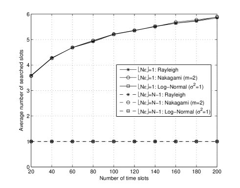
Figure 4: Average number of searched slots for the proposed algorithm under different fading scenarios

In Fig. 4, we investigate the average number of searched slots of Algorithm 1 and Algorithm 2, respectively, under different fading scenarios. In the simulation, $m=2$ is chosen for the unit-mean Nakagami fading channels used. For log-normal fading channels, $\sigma^{2}=1$ is used, with which the dB-spread will be within its typical ranges [30]. The average is taken over $10000$ channel realizations. It is observed from Fig. 4 that the average number of slots that the proposed algorithm has searched is almost the same for different fading scenarios. Besides, it is observed from Fig. 4 that the average number of searched slots of Algorithm 1 increases when the number of total slots increases. However, it increases at a very slow rate. It can be seen that the average number of searched slots is $6$ when the total number of slots is $200$. The average number of searched slots that Algorithm 2 has to search turns out to be one regardless of the number of total slots. This is due to the fact that since we only need to keep one slot, in most scenarios, the accumulated harvested energy is enough to support the channel inversion power of the slot with the highest channel power gains. For both cases, when the exhaustive search is adopted, the number of searched slots is $200$. This indicates that the proposed algorithms are highly efficient as compared to the exhaustive search whose complexity is linear.

VI-C General Case: $\lfloor N\epsilon\rfloor=M$

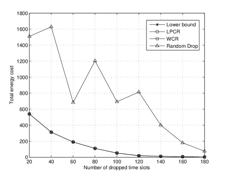
Figure 5: Comparison of the suboptimal algorithms with the lower bound

In this subsection, we consider the case that there are $200$ time slots. In Fig. 5, we plot the total energy cost vs. the number of dropped slots. The result is obtained by averaging over $1000$ channel realizations. The random drop algorithm, in which we drop the slots randomly and apply the greedy power allocation in the remaining time slots, is given as a baseline policy. From Fig. 5, it is observed that the performance of the random drop is the worst. This indicates that optimization contributes to significant energy saving for our problem. It is also observed that both the proposed suboptimal schemes, namely the LPCR and the WCR, can achieve almost the same performance as the lower bound. Furthermore, it is observed from Fig. 5 that the total energy cost decreases as the number of dropped slots increases for LPCR, WCR and the lower-bound, which is as expected. However, for the random drop, this does not hold. For example, the total energy cost of dropping $60$ slots can be lower than that of dropping $80$ slots. This can be explained as follows. In the random drop, since the slots are dropped randomly, it is possible that most of the $80$ dropped slots are with good channels and most of the $60$ dropped slots are with bad channels. As a result, the energy cost of dropping $60$ slots may be lower than that of dropping $80$ slots.

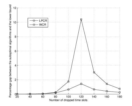
Figure 6: Gaps between the suboptimal algorithms and the lower bound

In Fig. 6, we plot the gap between the suboptimal schemes and the lower bound vs. the number of dropped slots. The result is obtained by averaging over 1000 channel realizations. It is observed that LPCR performs better than WCR in general. However, WCR performs close to the lower-bound when the number of slots to be dropped is either small (less than 80) or large (more than 160). For intermediate range (about 120 slots), WCR has about a $10\%$ gap from the lower bound. The intuition is as follows. When there are $200$ slots, it is likely that there will be a small number of slots that are in deep fading. At the optimal solution, these slots are likely to be dropped as the cost required to serve these slots is very high, even if all of them are using the cheap renewable energy. Similarly, it is also likely that there will be a number of slots in which the channel power gain is high, and these slots are likely to be kept as only a small amount of energy is needed to serve these slots. Since WCR is a greedy heuristic in which channels with low power gains are dropped, it is likely to agree with the optimal solution when the number of slots to be dropped is small or large. However, at the intermediate range, in addition to dropping the channels in deep fading and keeping channels with high power gains, we also have to make a decision on channels with moderate power gains. WCR only drops the channels with lower power gains, but does not take into account the renewable energy supply pattern. For channels with moderate power gains, the variation in the renewable energy supply may result in channels with lower power gains being kept in the optimal solution. This results in the sub-optimality of WCR. In contrast, in the LPCR algorithm, we try to take into account the variation in renewable energy through linear programming relaxation, resulting in a better performance in the intermediate range compared to WCR.

VI-D The multi-cycle case

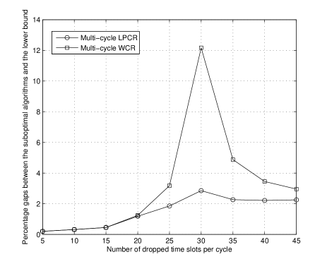
Figure 7: Gaps between the suboptimal algorithms and the lower bound: Multi-cycle case

In this case, we consider the case where there are in total $200$ time slots. These time slots are divided into $4$ cycles, and thus each cycle contains $50$ time slots. In Fig. 7, we plot the gap between the suboptimal schemes and the lower bound vs. the number of dropped slots in each cycle. The result is obtained by averaging over 1000 channel realizations. It is observed that the shape of the curves in this figure is similar to that of the curves in Fig. 6. Multi-cycle LPCR in general performs better than multi-cycle WCR. Multi-cycle WCR performs close to the lower-bound when the number of slots to be dropped is either small or large. This can be explained in the same way as the single-cycle case given in Section VI-C.

VI-E The partial CESI case

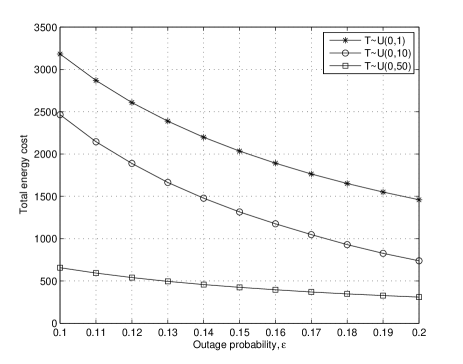
Figure 8: Performance for the proposed resource allocation scheme with partial CESI

In this subsection, we investigate the performance for the proposed resource allocation scheme with partial CESI. We consider the case that the channel fading statistics (i.e., exponentially distributed with mean $1$) are available at the Tx, while the energy harvesting state information is not known at the Tx. In Fig. 8, we plot the total energy cost of the proposed scheme vs. the given outage probability (i.e., $\epsilon$) under different energy harvesting profiles. It is observed that the total energy cost of all curves decrease with the increase of $\epsilon$. This is as expected since the transmit power is in general inversely proportional to $\epsilon$, which can be observed from (51). Another observation is that for the same $\epsilon$, the total energy cost under $T\sim\mathcal{U}(0,50)$ is lower than that under $T\sim\mathcal{U}(0,10)$. This indicates that the harvested energy plays a significant role in determining the energy cost.

VII Conclusions

In this paper, we have considered the problem of communicating over a block fading channel in which the transmitter has access to an energy harvester and a conventional energy source, and sought to minimize the total energy cost of the transmitter, subject to an outage constraint. This problem is shown to be a mixed integer programming problem. Optimal algorithms with worst case linear time complexity have been obtained in two extreme cases: when the number of slots in outage is $1$ or $N-1$. For the general case of allowing $1<k<N-1$ slots in outage, using a linear programming relaxation, we have obtained an efficiently computable lower bound as well as a suboptimal algorithm (upper bound), Linear Programming based Channel Removal (LPCR), for this problem. Using a greedy heuristic, we have also proposed another suboptimal algorithm with lower complexity, Worst-Channel Removal (WCR), and have shown that this algorithm is optimal under some channel conditions. Numerical simulations indicate that these algorithms exhibit only a small gap to the lower bound. Then, we show that the results obtained for the single-cycle case can be extended to the multi-cycle scenario with few modifications. Finally, when the only causal information on the energy arrivals and only channel statistics are available, we have introduced a new outage constraint and obtained the optimal resource allocation.

Appendix

VII-A Proof of Lemma 1

To prove Lemma 1, we verify the KKT conditions for the proposed policy. For $i\in\{1,2,\ldots,N\}$, we have

$$0\leq x_{i}^{*} \leq c_{i},$$ (58)

$$\sum_{i=1}^{k}x_{i}^{*}-\sum_{i=1}^{k}T_{i} \leq 0,$$ (59)

$$\lambda_{i}(x_{i}^{*}-c_{i}) =0$$ (60)

$$\mu_{i}(\sum_{j=1}^{i}x_{j}^{*}-\sum_{j=1}^{i}T_{j}) =0$$ (61)

$$\gamma_{i}x_{i}^{*} =0$$ (62)

$$-(\alpha-\beta)+\lambda_{i}+\sum_{j=i}^{N}\mu_{j}-\gamma_{i} =0$$ (63)

$$\lambda_{i}\geq 0,\mu_{i}\geq 0,\gamma_{i} \geq 0.$$ (64)

The first two conditions are satisfied since $x_{i}^{*}=\min\{c_{i},\sum_{j=1}^{i}T_{j}-\sum_{j=1}^{i-1}x^{*}_{j}\}$ is always chosen to be feasible. It remains to choose $\lambda_{i}$, $\mu_{i}$ and $\gamma_{i}$. To this end, we set $\gamma_{i}=0$. Let $K\in\{1,2,\ldots,N\}$ be the largest index such that $x_{K}^{*}=\sum_{j=1}^{K}T_{j}-\sum_{j=1}^{K-1}x_{j}^{*}$. If there is no such index, we set $K=0$. If $K>0$, we set $\mu_{K}=(\alpha-\beta)$ and $\mu_{i}=0$ for $i\neq K$; we set $\lambda_{i}=(\alpha-\beta)$ for $i>K$ and $\lambda_{i}=0$ for $i\leq K$. Note that $(\alpha-\beta)\geq 0$ since $\alpha\geq\beta$. Hence, these choices are feasible. If $K=0$, we set $\mu_{i}=0$ for all $i$ and $\lambda_{i}=(\alpha-\beta)$ for all $i$. It is now easy to verify that all the KKT conditions are satisfied.

VII-B Proof of Proposition 4

First, we consider the policy with initial storage state $S+\Delta$, i.e., $\pi(S+\Delta)$. Denote the conventional energy drawn at slot $i$ by $p_{i}^{c}(S+\Delta)$, and the energy drawn from the renewable by $p_{i}^{r}(S+\Delta)$. Then, it follows that

$$V(S+\Delta)=\sum_{i=1}^{n}\left(\alpha p_{i}^{c}(S+\Delta)+\beta p_{i}^{r}(S+\Delta)\right).$$ (65)

Now, we consider the policy with initial storage state $S$, i.e., $\pi(S)$. Let the storage state at slot $i$ be denoted by $E_{i}$. For convenience, we introduce the following indicator functions.

$$\chi_{i}=\left\{\begin{array}[]{ll}1,&\mbox{if}~{}p_{i}^{r}(S+\Delta)\leq E_{i-1}+T_{i},\\ 0,&\mbox{otherwise}.\end{array}\right.$$ (68)

$$\overline{\chi}_{i}=\left\{\begin{array}[]{ll}1,&\mbox{if}~{}p_{i}^{r}(S+\Delta)>E_{i-1}+T_{i},\\ 0,&\mbox{otherwise}.\end{array}\right.$$ (71)

Now, we drop the same time slot as in $\pi(S+\Delta)$. Then, the drawn energy under $\pi(S)$ can be written as follows,

$$p_{i}^{r}(S)=\chi_{i}p_{i}^{r}(S+\Delta)+\overline{\chi}_{i}\left(E_{i-1}+T_{i}\right),$$ (72)

$$p_{i}^{c}(S)=p_{i}^{c}(S+\Delta)+\overline{\chi}_{i}\left(p_{i}^{r}(S+\Delta)-E_{i-1}-T_{i}\right).$$ (73)

The overall cost of this policy is given by

$$V(S) =\sum_{i=1}^{n}\left(\alpha p_{i}^{c}(S)+\beta p_{i}^{r}(S)\right)$$

$$=\sum_{i=1}^{n}\alpha(p_{i}^{c}(S+\Delta)+\overline{\chi}_{i}(p_{i}^{r}(S+\Delta)-E_{i-1}-T_{i}))$$

$$+\beta(\chi_{i}p_{i}^{r}(S+\Delta)+\overline{\chi}_{i}(E_{i-1}+T_{i})).$$ (74)

Let $E^{\prime}_{i}$ be the storage state for slot $i$ under policy $\pi(S+\Delta)$. Now, we compute the cost difference between the two policies.

$$V(S)-V(S+\Delta)$$

$$=\sum_{i=1}^{n}\alpha(\overline{\chi}_{i}(p_{i}^{r}(S+\Delta)-E_{i-1}-T_{i}))$$

$$\quad+\beta\left((\chi_{i}-1)p_{i}^{r}(S+\Delta)+\overline{\chi}_{i}(E_{i-1}+T_{i})\right)$$

$$\stackrel{{\scriptstyle a}}{{=}}\sum_{i=1}^{n}(\alpha-\beta)(\overline{\chi}_{i}(p_{i}^{r}(S+\Delta)-E_{i-1}-T_{i}))$$

$$=\sum_{i=1}^{n}(\alpha-\beta)\Delta_{i},$$ (75)

where the equality “a” results from the fact that $\overline{\chi}_{i}=1-\chi_{i}$, and $\Delta_{i}=\overline{\chi}_{i}(p_{i}^{r}(S+\Delta)-E_{i-1}-T_{i})$.

Clearly, if $\overline{\chi}_{i}=0$, $\Delta_{i}=0$; if $\overline{\chi}_{i}=1$, $\Delta_{i}=p_{i}^{r}(S+\Delta)-E_{i-1}-T_{i}\stackrel{{\scriptstyle b}}{{=}}p_{i}^{r}(S+\Delta)-p_{i}^{r}(S)$, where the equality “b” results from the fact that $p_{i}^{r}(S)=E_{i-1}+T_{i}$ when $\overline{\chi}_{i}=1$ (observed from (72)). Hence, we have

$$V(S)-V(S+\Delta) =\sum_{i=1}^{n}(\alpha-\beta)\Delta_{i}\leq(\alpha-\beta)\Delta.$$ (76)

Proposition 4 is thus proved.

VII-C Proof of Proposition 5

Let $\mathcal{S}_{1}$ denote the set of slots that are kept in scheme 1, and $\mathcal{S}_{2}$ denote the set of slots that are kept in scheme 2. Denote the leftover harvested energy of scheme 1 as $L$, and that of scheme 2 as $\hat{L}$. Then, it follows that $L=\sum_{i=1}^{N}T_{i}-\sum_{i\in\mathcal{S}_{1}}p_{i}^{r}$, and $\hat{L}=\sum_{i=1}^{N}T_{i}-\sum_{i\in\mathcal{S}_{2}}\hat{p_{i}}^{r}.$ Then, we have

$$\Delta=\hat{L}-L =\left(\sum_{i=1}^{N}T_{i}-\sum_{i\in\mathcal{S}_{2}}\hat{p_{i}}^{r}\right)-\left(\sum_{i=1}^{N}T_{i}-\sum_{i\in\mathcal{S}_{1}}p_{i}^{r}\right)$$

$$=\sum_{i\in\mathcal{S}_{1}}p_{i}^{r}-\sum_{i\in\mathcal{S}_{2}}\hat{p_{i}}^{r}.$$ (77)

Denote the cost of scheme 1 and scheme 2 as $V$ and $\hat{V}$, respectively. Then, the cost difference of these two schemes are given as follows.

$$\hat{V}-V$$

$$= \sum_{i\in\mathcal{S}_{2}}\left(\alpha\hat{p}_{i}^{c}+\beta\hat{p}_{i}^{r}\right)-\sum_{i\in\mathcal{S}_{1}}\left(\alpha p_{i}^{c}+\beta p_{i}^{r}\right)$$

$$= \alpha\left(\sum_{i\in\mathcal{S}_{2}}\hat{p}_{i}^{c}-\sum_{i\in\mathcal{S}_{1}}p_{i}^{c}\right){\color[rgb]{0.00,0.00,0.00}+\beta\left(\sum_{i\in\mathcal{S}_{2}}\hat{p}_{i}^{r}-\sum_{i\in\mathcal{S}_{1}}p_{i}^{r}\right)}$$

$$= \alpha\left[\kern-1.42262pt\sum_{i\in\mathcal{S}_{2}}\kern-2.84526pt\left(\frac{N_{0}(e^{R}\kern-1.42262pt-\kern-1.42262pt1)}{g_{i}}\kern-1.42262pt-\kern-1.42262ptp_{i}^{r}\right)\kern-1.42262pt-\kern-2.84526pt\sum_{i\in\mathcal{S}_{1}}\kern-2.84526pt\left(\frac{N_{0}(e^{R}\kern-1.42262pt-\kern-1.42262pt1)}{g_{i}}\kern-1.42262pt-\kern-1.42262ptp_{i}^{r}\right)\kern-1.42262pt\right]{\color[rgb]{0.00,0.00,0.00}\kern-2.84526pt-\kern-1.42262pt\beta\Delta}$$

$$= \alpha\left(\sum_{i\in\mathcal{S}_{2}}\frac{N_{0}(e^{R}-1)}{g_{i}}-\sum_{i\in\mathcal{S}_{1}}\frac{N_{0}(e^{R}-1)}{g_{i}}\right)+\left(\alpha-\beta\right)\Delta.$$ (78)

It is clear that if scheme $1$ is WCR, we always have $\sum_{i\in\mathcal{S}_{1}}\frac{N_{0}(e^{R}-1)}{g_{i}}<\sum_{i\in\mathcal{S}_{2}}\frac{N_{0}(e^{R}-1)}{g_{i}}$. Consequently, we have that $\hat{V}-V>\left(\alpha-\beta\right)\Delta$. Thus, if WCR is the optimal solution for each individual cycle $i,~{}\forall i$, then it is clear that the multi-cycle WCR must be the optimal solution for Problem 6.

References

- [1] G. P. Fettweis and E. Zimmermann, “ICT energy consumption-trends and challenges,” in Proc. WPMC 2008.
- [2] G. Y. Li, Z. Xu, C. Xiong, C. Yang, S. Zhang, Y. Chen, and S. Xu, “Energy-efficient wireless communications: tutorial, survey, and open issues,” IEEE Wireless Commun., vol. 18, no. 6, pp. 28–35, Dec. 2011.
- [3] Y. Chen, S. Zhang, S. Xu, and G. Y. Li, “Fundamental trade-offs on green wireless networks,” IEEE Commun. Mag., vol. 49, no. 6, pp. 30–37, Jun. 2011.
- [4] J. P. Barton and D. G. Infield, “Energy storage and its use with intermittent renewable energy,” IEEE Trans. Energy Convers., vol. 19, no. 2, pp. 441–448, Jun. 2004.
- [5] O. Ozel and S. Ulukus, “Information-theoretic analysis of an energy harvesting communication system,” in Proc. IEEE PIMRC 2010, pp. 330–335.
- [6] R. Rajesh, V. Sharma, and P. Viswanath, “Capacity of fading Gaussian channel with an energy harvesting sensor node,” in Proc. IEEE GLOBECOM 2011, pp. 1–6.
- [7] J. Yang and S. Ulukus, “Optimal packet scheduling in an energy harvesting communication system,” IEEE Trans. Commun., vol. 60, no. 1, pp. 220–230, Jan. 2012.
- [8] K. Tutuncuoglu and A. Yener, “Optimum transmission policies for battery limited energy harvesting nodes,” IEEE Trans. Wireless Commun., vol. 11, no. 3, pp. 1180–1189, Mar. 2012.
- [9] C. K. Ho and R. Zhang, “Optimal energy allocation for wireless communications with energy harvesting constraints,” IEEE Trans. Signal Process., vol. 60, no. 9, pp. 4808–4818, Sept. 2012.
- [10] O. Ozel, K. Tutuncuoglu, J. Yang, S. Ulukus, and A. Yener, “Transmission with energy harvesting nodes in fading wireless channels: Optimal policies,” IEEE J. Sel. Areas Commun., vol. 29, no. 8, pp. 1732–1743, Sept. 2011.
- [11] J. Yang and S. Ulukus, “Optimal packet scheduling in a multiple access channel with energy harvesting transmitters,” Journal of Commun. and Netw., vol. 14, no. 2, pp. 140–150, Apr. 2012.
- [12] J. Yang, O. Ozel, and S. Ulukus, “Broadcasting with an energy harvesting rechargeable transmitter,” IEEE Trans. Wireless Commun., vol. 11, no. 2, pp. 571–583, Feb. 2012.
- [13] C. Huang, R. Zhang, and S. Cui, “Throughput maximization for the Gaussian relay channel with energy harvesting constraints,” Available at arXiv:1109.0724.
- [14] L. R. Varshney, “Transporting information and energy simultaneously,” in Proc. IEEE ISIT 2008, pp. 1612–1616.
- [15] P. Grover and A. Sahai, “Shannon meets Tesla: wireless information and power transfer,” in Proc. IEEE ISIT 2010, pp. 2363–2367.
- [16] R. Zhang and C. K. Ho, “MIMO broadcasting for simultaneous wireless information and power transfer,” IEEE Trans. Wireless Commun., vol. 12, no. 5, pp. 1989–2001, May 2013.
- [17] L. Liu, R. Zhang, and K.-C. Chua, “Wireless information transfer with opportunistic energy harvesting,” IEEE Trans. Wireless Commun., vol. 12, no. 1, pp. 288–300, Jan. 2013.
- [18] S. Luo, R. Zhang, and T. J. Lim, “Optimal save-then-transmit protocol for energy harvesting wireless transmitters,” IEEE Trans. Wireless Commun., vol. 12, no. 3, pp. 1196–1207, Mar. 2013.
- [19] X. Zhou, R. Zhang, and C. K. Ho, “Wireless information and power transfer: Architecture design and rate-energy tradeoff,” in Proc. IEEE GLOBECOM 2012, pp. 3982–3987.
- [20] X. Kang, C. K. Ho, and S. Sun, “Full-duplex wireless powered communication network with energy causality,” Available at arXiv:1404.0471.
- [21] Y.-K. Chia, S. Sun, and R. Zhang, “Energy cooperation in cellular networks with renewable powered base stations,” Available at arXiv:1301.4786.
- [22] D. W. K. Ng, E. S. Lo, and R. Schober, “Energy-efficient resource allocation in ofdma systems with hybrid energy harvesting base station,” IEEE Trans. Wireless Commun., vol. 12, no. 7, pp. 3412–3427, Jul. 2013.
- [23] O. Ozel, K. Shahzad, and S. Ulukus, “Optimal scheduling for energy harvesting transmitters with hybrid energy storage,” in Proc. IEEE ISIT 2013, pp. 1784–1788.
- [24] I. Ahmed, A. Ikhlef, D. W. K. Ng, and R. Schober, “Power allocation for an energy harvesting transmitter with hybrid energy sources,” IEEE Trans. Wireless Commun., vol. 12, no. 12, pp. 6255–6267, Dec. 2013.
- [25] C. H. Papadimitriou and K. Steiglitz, Combinatorial optimization : algorithms and complexity. Dover Publications Inc., 1998.
- [26] S. Boyd and L. Vandenberghe, Convex Optimization. Cambridge, UK: Cambridge University Press, 2004.
- [27] M. Grant and S. Boyd, “CVX: Matlab software for disciplined convex programming, version 2.0 beta,” Available at http://cvxr.com/cvx.
- [28] T. H. Cormen, C. E. Leiserson, R. L. Rivest, and C. Stein, Introduction to Algorithms. The MIT Press, 2009.
- [29] C. K. Ho, D. K. Pham, and C. M. Pang, “Markovian models for harvested energy in wireless communications,” in Proc. IEEE ICCS 2010, pp. 311–315.
- [30] X. Kang, Y.-C. Liang, A. Nallanathan, H. K. Garg, and R. Zhang, “Optimal power allocation for fading channels in cognitive radio networks: Ergodic capacity and outage capacity,” IEEE Trans. Wireless Commun., vol. 8, no. 2, pp. 940–950, Feb. 2009.