An ecoepidemic food chain with the disease at the intermediate trophic level

Abstract

We consider a three-level food chain in which an epidemics affects the intermediate population. Two models are presented, respectively either allowing for unlimited food supply for the bottom prey, or instead assuming for it a logistic growth. Counterintuitive results related to the paradox of enrichment are obtained, showing that by providing large amounts of food to the bottom prey, the top predator and the disease in suitable situations can be eradicated.

Keywords: epidemics, food chain, disease transmission, ecoepidemics AMS MR classification 92D30, 92D25, 92D40

1 Introduction

Food chains constitute a very common ecological situation. For an earlier model of this kind, see for instance [6]. In [12], a whole wealth of real life examples are presented and discussed. In particular, [5] contains a description of a cascade of diseases that moved from rinderpest for cattle to wild animals and then because of the death of these herds, caused also human diseases including smallpox. The study focuses on the reforestation of the Serengeti Woodlands along the past century. In it not only the role of fires in altering the landscape is described, but also the more relevant one of elephants. These animals stip the bark of trees and break their branches, contributing substantially to their decline. This behavior is common to several herbivores at all latitudes, [14, 15]. Also, the influence of the tsetse fly as carriers of the related infections of trypanosomes are highlighted. This disease affects large animals like cattle, but does not harm the small herbivores. It is the cause in man of the “sleeping sickness” disease. Overgrazing of cattle removes high quantities of grass and makes fires occurrence less frequent so that bushes can regrow. There seems to be a cyclic behavior among these phases (trees and tsetse, grass and fires) along the past century, evidence of a dynamic ecosystem, very much intricated.

In another investigation about the Serengeti Woodlands, [9], it is observed again that the reforestation is tightly related to diseases of wild animals populating or invading that environment, and therefore diseases, in this specific case rinderpest, play an essential role in regulating the ecosystem. Occurrence of epidemics among the herbivores has far reaching consequences not just for the animals, but also inflence the whole ecosystem via a kind of chain reaction. At the same time wild fires clearly control the canopy, changing the size of Carbon stored in the soil and the biomass.

Mathematical models for diseases affecting interacting populations are known since two decades at least, [7, 2, 16, 17], and involve interactions of every possible kind, [3, 18, 19, 20, 13] and various other modeling assumptions, [1, 8]. Ecoepidemiology, see Chapter 7 of [10], is the study of such ecosystems. So far, investigations have confined themselves essentially to simple systems, mainly two intermingling populations with one disease affecting one of them. But very recently epidemics in food chains have been considered, [4].

In this paper we continue the investigations of [4], in which the epidemics propagates instead at the lowest trophic level, by considering the infected individuals to be predators on the bottom prey, but also subject themselves to being hunted by a top predator.

Two models are here presented, after that the underlying basic demographic system is analysed, and then in turn the Malthus and the logistic versions of the ecoepidemic food chains are studied. A final interpretation of the results concludes the paper.

2 The general model

We consider a three trophic level food chain, composed by the populations $P,$ $H$ and $V$, in which the intermediate population is subject to a disease transmissible by contact at rate $\beta$. We therefore partition it into the two sets of susceptibles $S$ and infected $I$. We assume the disease to be unrecoverable. Also, it is confined to the population $H$ and cannot be trasmitted either to its predators $P$ or its prey $V$. The infected are weakened by the disease so much so as to be unable to extert any pressure on the population $V$, nor to feel any such pressure from the healthy individuals of their own population; they can be captured by the top predators but do not cause them any harm. The top predators do not have any food sources other than their prey $H$.

The model in the logistic formulation is

$$\begin{split}\frac{dP}{dt}&=P\left(gI+fS-\tau\right),\\ \frac{dS}{dt}&=S\left(lV-\beta I-qP-\mu\right),\\ \frac{dI}{dt}&=I\left(\beta S-cP-\nu\right),\\ \frac{dV}{dt}&=V\left[r\left(1-\frac{V}{K}\right)-bS\right].\end{split}$$ (1)

The first equation states that the top predators in absence of $H$ would die out at an exponential rate. They can survive by predation on the next trophic level, and as stated are not harmed by eating infected individuals. In the second equation we find the dynamics of the healthy individuals of the intermediate population. They reproduce as long as they can feed on the lower population $V$, and leave this class either by becoming infected, or by mortality, whether be it natural or induced by their capture from the top predators. The next equation contains the infected behavior; the only input is due to the $S$ individuals that become diseased upon “successful” contact with a disease-carrier. Infected leave this class if they are hunted by the $P$’s, or by mortality, which can also be induced by the disease. The last equation states that the lower population in the trophic level reproduces logistically and is hunted only by the healthy individuals of the upper trophic level.

The meaning of the parameters is as follows: $r$ denotes the reproduction rate of the population $V$ and $K$ is its respective carrying capacity; $b$ is the hunting rate of $S$ on $V$; $\beta$ is the disease incidence rate; $c$ and $q$ are the predation rate of $P$ on $I$ and $S$ respectively; $\mu$ is the population $H$ natural mortality rate, while $\nu:=\mu+\mu_{0}$ represents the mortality rate for the infected, which includes the disease-related mortality $\mu_{0}$; finally $\tau$ is the mortality rate for the population $P$. In view that not all prey are converted into predator’s biomass, we have the restrictions

$$g<c,\quad f<q,\quad l<b.$$ (2)

When the resources for $V$ are unlimited, i.e. for $K\rightarrow\infty$, we have the Malthus case, i.e. (1) simplifies as follows:

$$\begin{split}\frac{dP}{dt}&=gPI+fPS-\tau P,\\ \frac{dS}{dt}&=lSV-\beta SI-qSP-\mu S,\\ \frac{dI}{dt}&=\beta IS-cIP-\nu I,\\ \frac{dV}{dt}&=rV-bVS.\end{split}$$ (3)

The Jacobian $J$ of (1) is

$$\left[\begin{array}[]{cccc}gI+fS-\tau&fP&gP&0\\ -qS&lV-\mu-\beta I-qP&-\beta S&lS\\ -Ic&\beta I&-\nu+\beta S-cP&0\\ 0&-Vb&0&r(1-\frac{V}{K})-bS-\frac{Vr}{K}\end{array}\right]$$ (4)

Note that the Jacobian of (3) contains a modification only in the last term of the last equation, namely

$$J=\left[\begin{array}[]{cccc}gI+fS-\tau&fP&gP&0\\ -qS&lV-\mu-\beta I-qP&-\beta S&lS\\ -Ic&\beta I&-\nu+\beta S-cP&0\\ 0&-Vb&0&r-bS\end{array}\right].$$ (5)

3 The disease-free model

We replace the two intermediate equations of (1) by their total population $Q=S+I$, and observing that there are no infected in this case, in fact $Q=S$, thus obtaining the equation

$$\frac{dQ}{dt}=-\mu Q-qQP+lQV$$

Also, the Jacobian becomes a $3\times 3$ matrix. Corresponding changes occur in (3) and (5).

The system has only three meaningful equilibria, since the origin is unconditionally unstable. The bottom prey-only equilibrium $D_{1}=(0,0,K)$ exists only in the logistic case. The top-predator-free equilibrium $\widehat{D}=\left(0,\widehat{Q},\widehat{V}\right)$,

$$\widehat{Q}=\frac{r}{b}\left(1-\frac{\mu}{lK}\right),\quad\widehat{V}=\frac{\mu}{l}$$

and the coexistence equilibrium $D^{*}=\left(P^{*},Q^{*},V^{*}\right)$, whose population values are

$$P^{*}=\frac{1}{q}\left[lK\left(1-\frac{b\tau}{rf}\right)-\mu\right],\quad Q^{*}=\frac{\tau}{f},\quad V^{*}=K\left(1-\frac{b\tau}{rf}\right).$$

Now, $D_{1}$ is stable if

$$1>\frac{lK}{\mu}\equiv\rho_{1},$$ (6)

while $\widehat{D}$ is feasible in the opposite case,

$$\rho_{1}\geq 1.$$ (7)

Thus we have a transcritical bifurcation. $\widehat{D}$ is stable for

$$1>\frac{fr}{b\tau}\left(1-\frac{\mu}{lK}\right)\equiv\rho_{2}.$$ (8)

The opposite condition provides instead feasibility for $D^{*}$:

$$\rho_{2}\geq 1,$$ (9)

thus we have another transcritical bifurcation. Stability of $D^{*}$ holds unconditionally, whenever the equilibrium is feasible, as the Routh-Hurwitz conditions become

$$\frac{r}{K}V^{*}>0,\quad fq\frac{r}{K}P^{*}Q^{*}V^{*}>0,\quad blV^{*}>0.$$ (10)

4 The Malthus case

For the ecoepidemic cases, we analyse at first the particular case of (1).

The possible equilibria are the following points: since the system is homogeneous, the origin trivially satisfies it, $\widetilde{E}_{0}=(0,0,0,0)$. Then we have

$$\widetilde{E}_{1}=\left(0,\frac{r}{b},0,\frac{\mu}{l}\right)$$

which is always feasible. Finally, coexistence is obtained at the level

$$\widetilde{E}^{*}=\left(\frac{\beta r-\nu b}{bc},\frac{r}{b},\frac{b\tau-rf}{gb},\frac{\beta rgq-\beta rfc+bg\mu c-bgq\nu+b\tau\beta c}{gbcl}\right).$$ (11)

Feasibility implies that all the following conditions hold

$$\frac{r\beta}{b\nu}\geq 1;\quad\frac{rf}{b\tau}\leq 1;\quad b\frac{\tau\beta c+g\left(\mu c-q\nu\right)}{r\beta\left(fc-gq\right)}\leq 1.$$ (12)

Remark 1. It is interesting to note that the bottom population-free point

$$\left(-\frac{\nu f-g\mu-\tau\beta}{-gq+fc},\frac{g\mu c-gq\nu+\tau\beta c}{\beta(-gq+fc)},-\frac{\mu cf-q\nu f+q\tau\beta}{\beta\left(-gq+fc\right)},0\right)$$

intuitively cannot be an equilibrium, since what is called the primary producer, $V$, is wiped out, and therefore the first trophic level, i.e. populations $S$ and $I$ that feed on it, cannot thrive any longer, and in turn also the top predator must die out, since the intermediate population is depleted. This observation has its counterpart in the mathematics, since this point is not feasible. In fact requiring all its populations to be nonnegative leads to the two mutually exclusive conditions

$$\frac{g}{c}>-\frac{\tau\beta}{\mu c-q\nu};\qquad\frac{g}{c}<-\frac{\tau\beta}{\mu c-q\nu}.$$

Remark 2. Some similar considerations can be made in a few other cases. In particular note that for the top predator-free subsystem cannot settle to an equilibrium, quite unexpectedly, because removing the $P$ population and its related differential equation, we find from the last two equilibrium equations that $S$ attains the values

$$S=\frac{\nu}{\beta},\quad S=\frac{r}{b}$$

which cannot be equal except for a very restrictive condition on the parameters, that in general does not hold.

Easily, the eigenvalues of the Jacobian (5) at the origin are $-\nu$, $-\tau$, $-\mu$, $r$, from which instability of $\widetilde{E}_{0}$ follows.

At $\widetilde{E}_{1}$ we find

$$\pm i\sqrt{\mu r},\quad\frac{\beta r-\nu b}{b},\quad\frac{rf-b\tau}{b}.$$

It follows that if we require

$$\frac{r\beta}{b\nu}<1,\quad\frac{rf}{b\tau}<1$$ (13)

we obtain the neutral, or center, stability, since the remaining two eigenvalues are pure imaginary. This feature is of course inherited by the fact that the underlying demographic model in this case is the classical Lotka-Volterra predator-prey model. On comparing the first stability condition (13) with the first feasibility condition (12) of $\widetilde{E}^{*}$, we discover a transcritical bifurcation for which coexistence originates from the equilibrium $\widetilde{E}_{1}$ when the latter becomes unstable.

The equilibrium $\widetilde{E}^{*}$ exhibits a fourth degree characteristic polynomial,

$$\sum_{k=0}^{4}a_{4-k}\lambda^{k},\quad a_{0}=1,$$ (14)

with known but rather complicated coefficients, which we omit. In any case, we find that $a_{1}=0$, so that the very first Routh-Hurwitz condition, $a_{1}>0$ is not satisfied. We conclude then that $\widetilde{E}^{*}$ is always unstable.

Coexistence then can only occur at unstable level, i.e. via oscillations. This is shown in Figure 1 for the parameter values $g=0.3$, $f=0.2$, $c=0.4$, $l=0.2$, $q=0.3$, $b=0.4$, $\beta=0.3$, $\tau=0.4$, $\nu=0.3$, $\mu=0.2$, $r=0.5$.

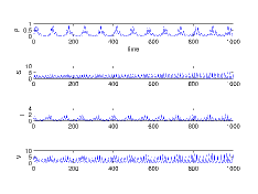
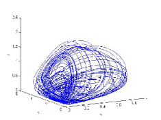
Figure 1: Coexistence is attained through persistent oscillations. Left: the populations as function of time, $P$, $S$, $I$, $V$ from top to bottom. Right: the $PSI$-subspace phase portrait of the system trajectories. Parameter values: $g=0.3$, $f=0.2$, $c=0.4$, $l=0.2$, $q=0.3$, $b=0.4$, $\beta=0.3$, $\tau=0.4$, $\nu=0.3$, $\mu=0.2$, $r=0.5$.

5 The logistic case

We now consider (1). In this case it is possible to show boundedness of the system.

Theorem. The system’s trajectories are bounded.

Proof. Let us consider the total environment population, $W=P+S+I+V$. Upon summation of the equations in (1) we obtain,

$$\frac{dW}{dt}=(g-c)PI+(f-q)PS+(l-b)SV-\tau P-\mu S-\nu I+rV\left(1-\frac{V}{K}\right).$$

Recalling the relationships between parameters (2), introducing an arbitrary $\theta>0$, we find

$$\frac{dW}{dt}+\theta W\leq-(\tau-\theta)P-(\mu-\theta)S-(\nu-\theta)I+(r+\theta)V-\frac{r}{K}V^{2}.$$

Taking $\theta\leq\min\{\tau,\mu,\nu\}$, the first terms in the above inequality can be dropped. The last two terms are the parabola $\Psi(V)=V[(r+\theta)-rVK^{-1}]$, whose vertex lies at the point $(V_{0},\Psi^{*})=\left((r+\theta)K(2r)^{-1},(r+\theta)^{2}K(4r)^{-1}\right)$. It therefore follows

$$\frac{dW}{dt}+\theta W\leq\Psi^{*}$$

and upon integration of the corresponding differential equation we find $W(t)=\Psi^{*}\theta^{-1}[1-\exp(-\theta t)]+W(0)\exp(-\theta t)$ so that ultimately

$$W(t)\leq\max\left\{W(0),\frac{\Psi^{*}}{\theta}\right\},$$

as desired.

The equilibria are once again the origin $E_{0}$ and the equilibrium of the lowest two trophic levels predator-prey disease-free subsystem, $E_{1}$, for which now the susceptible population level is lower than in the Malthus case $\widetilde{E}_{1}$, namely

$$S_{1}=\frac{r}{b}\left(1-\frac{\mu}{lK}\right),\quad V_{1}=\frac{\mu}{l},$$

and $E^{*}$, whose components cannot in this case be explicitly evaluated. Feasibility for $E_{1}$ holds if (7) is satisfied. In addition, we find the bottom-prey-only equilibrium $E_{2}=(0,0,0,K)$ and two more points,

$$E_{3}=\left(0,\frac{\nu}{\beta},\frac{lKr\beta-lKbv-\mu r\beta}{r\beta^{2}},K\frac{r\beta-b\nu}{r\beta}\right)$$

the top-predator free equilibrium and the disease-free equilibrium

$$E_{4}=\left(\frac{rflK-rf\mu-\tau lKb}{rfq},\frac{\tau}{f},0,K\frac{rf-b\tau}{rf}\right).$$

To have nonnegative populations, we must impose both the following feasibility conditions

$$r\beta(KL-\mu)>bKl\nu.$$ (15)

Similarly, for feasibility of $E_{4}$ the parameters must instead satisfy

$$rf(KL-\mu)>bKl\tau.$$ (16)

The eigenvalues at $E_{0}$ coincide with those of $\widetilde{E}_{0}$, so that the origin retains its unstable character.

At $E_{2}$ we find the eigenvalues $-r$, $-\nu$, $-\tau$, $lK-\mu$. It is stable if (6) holds, which compared with the feasibility condition for $E_{1}$, (7), shows again the existence of a transcritical bifurcation, inherited from the demographic model.

For $E_{1}$ things change a bit, with respect to $\widetilde{E}_{1}$. Namely the coefficients of the characteristic equation (14) are now

$$a_{4}=\frac{(-rflK+rf\mu+\tau lKb)r(lK-\mu)\mu(-lKr\beta+lKb\nu+\mu r\beta)}{l^{3}K^{3}b^{2}},$$

$$a_{3}=\frac{\mu r}{l^{3}K^{3}b^{2}}(-rfl^{3}K^{3}b+2rfl^{2}K^{2}b\mu+r^{2}fl^{2}K^{2}\beta-rfl^{2}K^{2}b\nu-2r^{2}flK\mu\beta$$

$$-rf\mu^{2}lKb+rf\mu lKb\nu+r^{2}f\mu^{2}\beta+\tau l^{3}K^{3}b^{2}-\tau l^{2}K^{2}b^{2}\mu-\tau l^{2}K^{2}br\beta$$

$$+\tau l^{2}K^{2}b^{2}\nu+\tau lKb\mu r\beta-l^{3}K^{3}br\beta+l^{3}K^{3}b^{2}\nu+2l^{2}K^{2}b\mu r\beta-l^{2}K^{2}b^{2}\mu\nu$$

$$-lKb\mu^{2}r\beta),$$

$$a_{2}=\frac{1}{l^{2}K^{2}b^{2}}(r^{2}fl{2}K^{2}\beta-rfl^{2}K^{2}b\nu-2r^{2}flK\mu\beta-r^{2}flK\mu b+rf\mu lKb\nu$$

$$+r^{2}f\mu^{2}\beta+r^{2}f\mu^{2}b-\tau l^{2}K^{2}br\beta+\tau l^{2}K^{2}b^{2}\nu+\tau lKb\mu r\beta+\tau lKb^{2}\mu r$$

$$+\mu rb^{2}l^{2}K^{2}-\mu^{2}rb^{2}lK-\mu r^{2}blK\beta+\mu rb^{2}lK\nu+\mu^{2}r^{2}b\beta),$$

$$a_{1}=\frac{1}{lkb}(-rflK+rf\mu+\tau lKb-lKr\beta+lKbv+\mu r\beta).$$

In this case the analysis of the Routh-Hurwitz conditions is far from being easy.

The case of the equilibria $E_{3}$ and $E_{4}$ leads to similar very complicated expressions for the coefficients of the characteristic polynomial (14), which we omit altogether. In the simulations, we show that all these last three points can be attained by the system’s trajectories at a stable level, for suitable parameter choices. These are illustrated in Figures 2, 3, 4.

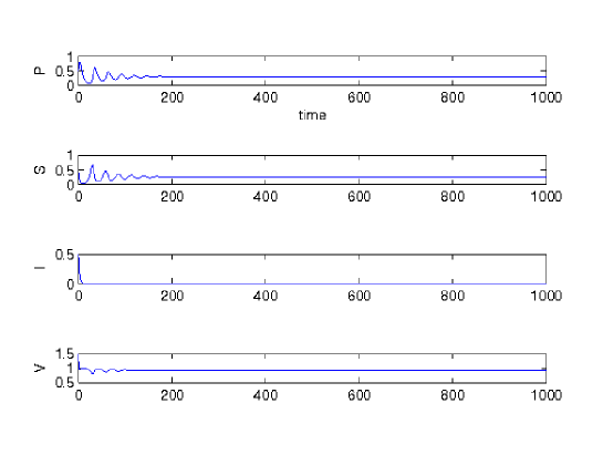
Figure 2: The disease-free equilibrium $E_{4}=(0.3,0.25,0,1.0)$, attained in the logistic case for the parameter values $g=0.3$, $f=0.2$, $c=0.4$, $l=0.6$, $q=0.7$, $b=0.9$, $\beta=0.1$, $\tau=0.2$, $\nu=0.2$, $\mu=0.2$, $r=1.3$, $K=1.0$.

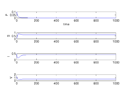
Figure 3: The top predator-free equilibrium $E_{3}=(0,0.6667,0.4103,0.5385)$ stably attained for the parameter values $g=0.3$, $f=0.1$, $c=0.4$, $l=0.6$, $q=0.7$, $b=0.9$, $\beta=0.3$, $\tau=0.2$, $\nu=0.2$, $\mu=0.2$, $r=1.3$, $K=1.0$.

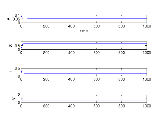
Figure 4: The coexistence equilibrium $E^{*}=(0.0571,0.7429,0.1714,0.4857)$ stably attained in the logistic model for the parameter values $g=0.3$, $f=0.2$, $c=0.4$, $l=0.6$, $q=0.7$, $b=0.9$, $\beta=0.3$, $\tau=0.2$, $\nu=0.2$, $\mu=0.2$, $r=1.3$, $K=1.0$.

6 Discussion

We have investigated a three trophic level ecoepidemic food chain, in which the disease affects the population at the intermediate trophic level. In all models the origin is unstable, this essentially stems from the demographic assumptions, and represents a good property of the ecosystem, showing that it cannot be completely wiped out.

The purely demographic model admits the following equilibria: the bottom prey-only equilibrium, which however exists at a finite level only in the logistic case, the equilibrium with the bottom prey and the intermediate predator, and coexistence. These equilibria are related to each other via two transcritical bifurcations, which occur whenever the parameters $\rho_{1}$ and $\rho_{2}$ cross the critical value 1. In those cases, the intermediate predator and top predator respectively enter permanently into the system.

In the ecoepidemic models again these purely demographic, disease-free, equilibria can be found, in particular we observe again that the bottom prey-only equilibrium exists just in the logistic version.

A very interesting situation occurs in (3). The demographic coexistence equilibrium in the Malthus version of the ecoepidemic model is not found. The latter is always unstable, so that the three populations persist with an endemic disease only via sustained oscillations. Thus introducing a transmissible disease in a food chain model of this type has the effect that the disease either enters endemically in the system, or it removes one trophic level, specifically the uppermost one, if the stability conditions of equilibrium $\widetilde{E}_{1}$ are satisfied, namely (13).

Alternatively, we can rephrase this concept in a different way. The only possibility for the disease to be endemic occurs whenever the coexistence equilibrium is attained. No subsystem allows the disease to be present in it. Therefore in this system the task of eradicating the epidemics is intimately tied to the disappearance of at least one trophic level. Specifically, it will be the top predator, at the stable equilibrium $\widetilde{E}_{1}$, or possibly at the closed orbits centered around it. This is counterintuitive, since one expects the top predator to have a positive role in the disease containment. In fact naively we could think that by hunting diseased individuals it would contain the epidemics spread.

The same result instead does not hold for the logistic system, we find indeed both the three-level disease-free food chain equilibrium $E_{4}$ and the subsystem made of the lowest two trophic levels with endemic disease, equilibrium $E_{3}$.

Upon comparison of the two situations, we can conclude thus that providing more food for the bottom prey, i.e. driving the logistic system toward the Malthus model, may help in disease eradication, but also may drive to extinction the top predator. This could be regarded as an alternative formulation of the paradox of enrichment, by which by feeding the prey one kills the predators. However, this phenomenon in the present situation is to be ascribed to the demographic model and not to the disease, as the same occurs in the epidemic-free model. In it, by providing large amount of food for the bottom prey the bottom prey-only equilibrium $D_{1}$ disappears, and the system can settle either to coexistence or to the top predator-free equilibrium $D_{2}$, depending on the value of the critical parameter $\rho_{2}$, since the stability conditions (10) are always satisfied for the coexistence equilibrium. Instead, in the ecoepidemic model either all the populations of the system, infected included, oscillate, or the top predator-free equilibrium is attained by imposing condition (7).

References

- [1] O. Arino, A. El Abdllaoui, J. Mikram, J., Chattopadhyay, Infection on prey population may act as a biological control in ratio-dependent predator-prey model, Nonlinearity, 17, (2004) 1101-1116.
- [2] E. Beltrami, T.O., Carroll, Modelling the role of viral disease in recurrent phytoplankton blooms, J. Math. Biol. 32, (1994) 857-863.
- [3] J. Chattopadhyay, O. Arino, A predator prey model with disease in the prey, Nonlinear Analysis 36 (1999) 747-766.
- [4] A. De Rossi, F. Lisa, L. Rubini, A. Zappavigna, E. Venturino, A food chain ecoepidemic model: infection at the bottom trophic level submitted to ECOCOM, http://arxiv.org/abs/1403.0869
- [5] H.T. Dublin, Dynamics of the Serenget 1-Mara Woodlands An Historical Perspective, Forest and Conservation History 35 (1991) 169-178.
- [6] T.C. Gard, T.G. Hallam, Persistence in food web -1, Lotka- Volterra food chains, Bull Math Bio 41, (1979) 877-891.
- [7] K.P. Hadeler, H.I. Freedman, (1989), Predator-prey populations with parasitic infection, J. of Math. Biology 27, 609-631.
- [8] M. Haque, E. Venturino, An ecoepidemiological model with disease in the predator; the ratio-dependent case, Math. Meth. Appl. Sci. 30, 1791-1809, 2007.
- [9] R.M. Holdo, A.R.E. Sinclair, A.P. Dobson, K.L. Metzger, B.M. Bolker, et al. A Disease-Mediated Trophic Cascade in the Serengeti and its Implications for Ecosystem C. PLoS Biol 7(9) (2009): e1000210. doi:10.1371/journal.pbio.1000210
- [10] H. Malchow, S. Petrovskii, E. Venturino, Spatiotemporal patterns in Ecology and Epidemiology, CRC, 2008, 442 pp.
- [11] T. Sato, T. Egusa, K. Fukushima, T. Oda, N. Ohte, N. Tokuchi, K. Watanabe, M. Kanaiwa, I. Murakami, K.D. Lafferty, Nematomorph parasites indirectly alter the food web and ecosystem function of streams through behavioural manipulation of their cricket hosts, Ecology Letters, 15: (2012) 786-793
- [12] Selakovic, S., de Ruiter, P. C., Heesterbeek, H., Infection on prey population may act as a biological control in ratio-dependent predator-prey model, Proc. R. Soc. B, 281, (2014) online 20132709.
- [13] M. Sieber, F.M. Hilker, Prey, predators, parasites: intraguild predation or simpler community modules in disguise?, Journal of Animal Ecology 80, (2011) 414-421.
- [14] L. Tamburino, V. La Morgia, E. Venturino, System dynamic approach to management of urban parks. A case study: the Meisino urban park in Torino, NW Italy, Computational Ecology and Software, 2(1) (2012) 26-41.
- [15] L. Tamburino, E. Venturino, Public parks management via mathematical tools, Int. J. Comp. Math. 89(13-14) (2012) 1808-1825.
- [16] E. Venturino, The influence of diseases on Lotka-Volterra systems, Rocky Mountain Journal of Mathematics, vol. 24, p. 381-402, 1994, IMA preprint #951, Minneapolis, MN, 1992.
- [17] E. Venturino, Epidemics in predator-prey models: disease among the prey, in O. Arino, D. Axelrod, M. Kimmel, M. Langlais: Mathematical Population Dynamics: Analysis of Heterogeneity, Vol. one: Theory of Epidemics, Wuertz Publishing Ltd, Winnipeg, Canada, p. 381-393, 1995.
- [18] E. Venturino, The effects of diseases on competing species, Math. Biosc. 174 (2001) 111-131.
- [19] E. Venturino, Epidemics in predator-prey models: disease in the predators, IMA Journal of Mathematics Applied in Medicine and Biology 19, (2002) 185-205.
- [20] E. Venturino, How diseases affect symbiotic communities, Math. Biosc. 206 (2007) 11-30.