Valley-antisymmetric potential in graphene under dynamical deformation

Abstract

When graphene is deformed in a dynamical manner, a time-dependent potential is induced for the electrons. The potential is antisymmetric with respect to valleys, and some straightforward applications are found for Raman spectroscopy. We show that a valley-antisymmetric potential broadens Raman $D$ band but does not affect $2D$ band, which is already observed by recent experiments. The space derivative of the valley antisymmetric potential gives a force field that accelerates intervalley phonons, while it corresponds to the longitudinal component of the previously discussed pseudoelectric field acting on the electrons. Effects of a pseudoelectric field on the electron is quite difficult to observe due to the valley-antisymmetric coupling constant, on the other hand, such obstacle is absent for intervalley phonons with $A_{1g}$ symmetry that constitute the $D$ and $2D$ bands.

A lattice structure with exact periodicity, namely equal bond lengths for every bond species, does not exist in nature. Lattice deformation is inevitable even in a simple planar structure consisting of a single atom species, namely graphene. Novoselov et al. (2005); Zhang et al. (2005) Graphene research has already clarified that lattice deformation can be expressed by a gauge field. González et al. (1992); Kane and Mele (1997); Lammert and Crespi (2000); Sasaki et al. (2005); Jackiw and Pi (2007); Sasaki and Saito (2008); Vozmediano et al. (2010) A deformation-induced gauge field has been employed in predicting notable phenomena. For example, Landau levels, which are usually formed by applying a magnetic field to graphene, are also constructed by applying strain to graphene. The novel Landau levels were predicted in terms of a static strain-induced pseudomagnetic field, which is defined by the rotation of the gauge field by analogy with a magnetic field. Guinea et al. (2010); Levy et al. (2010) There is a crucial difference between magnetic and pseudomagnetic fields. Namely, the coupling constant of pseudomagnetic field has opposite signs for the electrons at different valleys (valley anti-symmetric), whereas the coupling constant of a magnetic field is the same for the valleys (valley symmetric).

Recently, some attempts have been made to understand the effects of dynamical (time-dependent) lattice deformation in terms of a pseudoelectric field, which is defined by the time derivative of the gauge field by analogy with an electric field. Vozmediano et al. (2010); Vaezi et al. (2013); Trif et al. (2013) A pseudoelectric field as well as a normal electric field can accelerate the electrons and induce current. However, since the coupling constant is valley anti-symmetric, the currents at the K and K’ valleys flow in the opposite directions and they cancel out. As a result of the cancellation effect, a pseudoelectric field does not cause a net electric current, in general. While several authors try to extract a net electric current from a time-dependent lattice deformation, such attempt is based on unrealistic assumptions. Vaezi et al. (2013)

In this paper, we show that the cancellation effect of a pseudoelectric field which originated from the valley-antisymmetric coupling constant, is absent for intervalley phonons. The phonons are observed in the Raman spectrum of graphene, and the effects of a pseudoelectric field are already visible from recent experiments of Raman spectroscopy. The point of our theoretical analysis is that a valley-antisymmetric potential is induced for the electrons when graphene is deformed in a dynamical manner, and the spatial derivative of the potential gives a force field for the phonons, which turns out to be the longitudinal component of the previously discussed pseudoelectric field acting on the electrons. In other words, we have extended the idea of a pseudoelectric field to include the phonons, by introducing the concept of a valley-antisymmetric potential acting on the electron. The force field on the phonons is free from the cancellation effect so that the effect of a pseudoelectric field is easy to observe.

Before providing an exact formulation of a valley-antisymmetric potential, we outline the main result here in such a way that readers will easily be able to grasp the essential points. When graphene is deformed in a time dependent manner, the electrons are subject to a potential. It is valley antisymmetric, that is, the sign of the potential is different for the K and K’ valleys as shown in Fig. 1(a). The potential is time dependent and disappears when the deformation becomes static as shown in Fig. 1(b). Meanwhile, static deformation causes a shift of the wavevector between the K and K’ points, which is permanent.

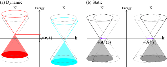
Figure 1: (a) A transient valley-antisymmetric potential is induced when lattice deformation is time dependent. (b) When the deformation becomes static, the potential disappears, while the positions of the K and K’ points are slightly shifted compared with those in the absence of deformation.

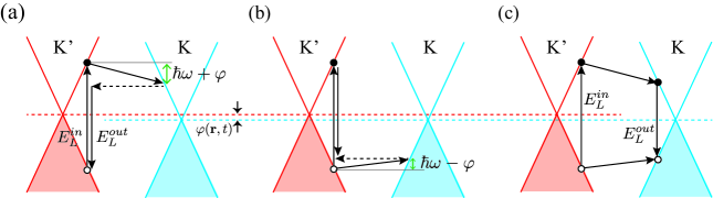
Figure 2: The origin of the $D$ band broadening in the presence of a valley-antisymmetric potential $\varphi$. (a) When a photo-excited electron experiences an intervalley scattering by emitting an $A_{1g}$ phonon with frequency $\omega$, the Raman shift $E_{L}^{in}-E_{L}^{out}$ is given by $\hbar\omega+\varphi$. (b) When a hole emits an $A_{1g}$ phonon, $E_{L}^{in}-E_{L}^{out}$ is given by $\hbar\omega-\varphi$. (c) There is no spectrum change for the $2D$ Raman band because of the cancellation: $E_{L}^{in}-E_{L}^{out}=(\hbar\omega+\varphi)+(\hbar\omega-\varphi)=2\hbar\omega$.

A straightforward application of a valley-antisymmetric potential is found with respect to the defect-induced $D$ band observed in the Raman spectrum of graphene. Tuinstra and Koenig (1970); Cançado et al. (2004); Sasaki et al. (2013) The Raman process starts when an electron-hole pair is created in the Dirac cones by absorbing a laser light, as shown in Fig. 2(a) and 2(b). A photo-excited electron or hole can change its valley by emitting an intervalley phonon, which constitutes the $D$ band. Elastic intervalley scattering (represented by dashed arrows) caused by certain defects, such as the armchair graphene edge, Cançado et al. (2004); Gupta et al. (2009); Sasaki et al. (2013) can compensate for the changes in the valleys. Then the electron recombines with the hole as the result of a scattered light emission, which completes the Raman process. Malard et al. (2009) Let $\omega$ and $\varphi$ be the frequency of the phonon and the potential difference, respectively. As shown in Fig. 2(a), the potential difference $\varphi$ contributes to the Raman shift, which is the energy difference between the incident and scattered light as $E_{L}^{in}-E_{L}^{out}=\hbar\omega+\varphi$. On the other hand, when the hole emits an intervalley phonon, the energy difference is $\hbar\omega-\varphi$ as shown in Fig. 2(b). Because the processes shown in Fig. 2(a) and 2(b) occur with equal probability, the $D$ band broadens in the Raman spectrum, provided that $\varphi$ is distributed in the spot of the laser light. The broadening is interpreted as the emission of a combination mode of the intervalley phonon and acoustic phonon, as shown later at Eq. (6). The $2D$ Raman band, which consists of two intervalley phonons, does not broaden even when $\varphi\neq 0$ because of the cancellation: $(\hbar\omega+\varphi)+(\hbar\omega-\varphi)=2\hbar\omega$, as shown in Fig. 2(c). The effect of a valley antisymmetric potential on the $2D$ band is in sharp contrast to that on the $D$ band.

Such $D$ and $2D$ Raman band behavior was observed in a recent Raman spectroscopy experiment. Suzuki et al. (2013) In the experiment, H₂O molecules are considered to be inserted between the graphene layer and substrate. When H₂O molecules are irradiated by a laser light, the interaction between H₂O molecules and graphene induces a time-dependent lattice deformation, which we identify as the origin of $\varphi$. The interaction between H₂O molecules and graphene is also discussed by Mitoma et al. Mitoma et al. (2013) The authors observed an enhancement of the $D$ band intensity for graphene on a water-rich substrate and explained it in terms of the photo-oxidation of graphene. For a strong laser light, the deformation can be significantly large and graphene may be further damaged by such dynamical deformation.

A valley antisymmetric potential and a shift of the K and K’ points are both described in a unified fashion by the formulation of a deformation-induced gauge field. When a C-C bond expands or shrinks in the graphene plane, the hopping integral diverges from the equilibrium value $-\gamma$. Porezag et al. (1995) Thus, lattice deformation is defined by a change in the hopping integral, which depends on the position of a carbon atom ${\bf r}$, the bond direction $a$ ($=1,2,3$), and time $t$, as $-\gamma+\delta\gamma_{a}({\bf r},t)$. In the absence of deformation, the low-energy dynamics of the $\pi$-electrons is governed by a massless Dirac equation. Novoselov et al. (2005); Zhang et al. (2005) Lattice deformation modifies the massless Dirac equation into a Dirac equation that includes a deformation-induced gauge field ${\bf A}^{q}({\bf r},t)$ and mass $m({\bf r},t)$ as Sasaki and Saito (2008)

$$i\hbar\frac{\partial}{\partial t}\begin{pmatrix}\Psi_{\text{K}}({\bf r},t)\cr\Psi_{\text{K}^{\prime}}({\bf r},t)\end{pmatrix}=\begin{pmatrix}v\mbox{\boldmath$\sigma$}\cdot(\hat{\bf p}+{\bf A}^{q}({\bf r},t))&m({\bf r},t)\sigma_{x}\cr m({\bf r},t)^{*}\sigma_{x}&v\mbox{\boldmath$\sigma$}^{\prime}\cdot(\hat{\bf p}-{\bf A}^{q}({\bf r},t))\end{pmatrix}\begin{pmatrix}\Psi_{\text{K}}({\bf r},t)\cr\Psi_{\text{K}^{\prime}}({\bf r},t)\end{pmatrix}.$$ (1)

In this equation, $v\sim 10^{6}$ m/s is the velocity of the electron, $\hat{\bf p}=-i\hbar\nabla$ is the momentum operator, $\mbox{\boldmath$\sigma$}=(\sigma_{x},\sigma_{y})$ and $\mbox{\boldmath$\sigma$}^{\prime}=(-\sigma_{x},\sigma_{y})$ are the Pauli matrices that operate on the two-component wavefunction for each valley, $\Psi_{\text{K}}$ or $\Psi_{\text{K}^{\prime}}$. The mass is induced when the lattice deformation has a short distance periodicity comparable to the lattice constant. In the lattice vibrational motions in graphene, such deformation appears as an intervalley phonon with $A_{1g}$ symmetry. Tuinstra and Koenig (1970); Malard et al. (2009); Cançado et al. (2004); Sasaki et al. (2013) Let ${\bf k}_{F}+{\bf q}$ be the wavevector of an $A_{1g}$ phonon, where ${\bf k}_{F}$ denotes the wavevector of the K point, and $\omega$ is the frequency, it can be shown that $m({\bf r},t)=m_{0}e^{i{\bf q}\cdot{\bf r}}\cos(\omega t)$, where $m_{0}$ is a constant determined by the electron-phonon coupling $g\sim 6$ eV. Meanwhile, the field ${\bf A}^{q}({\bf r},t)=(A_{x}^{q}({\bf r},t),A_{y}^{q}({\bf r},t))$ is calculated from the displacement vector of the acoustic phonons ${\bf u}({\bf r},t)=(u_{x}({\bf r},t),u_{y}({\bf r},t))$ by $vA_{x}^{q}({\bf r},t)=g(-\partial_{x}u_{x}({\bf r},t)+\partial_{y}u_{y}({\bf r},t))/2$ and $vA_{y}^{q}({\bf r},t)=g(\partial_{y}u_{x}({\bf r},t)+\partial_{x}u_{y}({\bf r},t))/2$ (See Sec.I of Supplementary Materials for details). Some examples of static gauge field ${\bf A}^{q}({\bf r})$ are shown in Fig. 3.

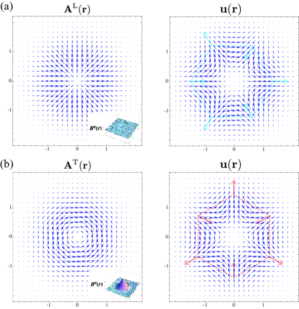
Figure 3: (a,left) Plot of longitudinal deformation-induced gauge field ${\bf A}^{\rm L}({\bf r},t)=\nabla\Phi({\bf r})$ with $\Phi({\bf r})\propto-e^{-({\bf r}/\ell)^{2}}$. Note that when we assume that ${\bf A}^{q}({\bf r},t)=\nabla\Phi({\bf r})\cos(\omega t)$, the vector field also represents the pseudoelectric field ${\bf E}^{q}({\bf r},t)$. The inset shows the pseudomagnetic field $B^{q}({\bf r})$ which is zero for ${\bf A}^{\rm L}({\bf r},t)$. (a,right) The corresponding displacement vector field ${\bf u}({\bf r})$. The arrows represent the direction of the field at the points. (b,left) Plot of transverse gauge field ${\bf A}^{\rm T}({\bf r},t)=(\partial_{y},-\partial_{x})\Phi({\bf r})$. The inset shows the plot of pseudomagnetic field $B^{q}({\bf r})\neq 0$. (b,right) The corresponding displacement vector field ${\bf u}({\bf r})$.

The crucial step in clarifying the effect of the time dependence of lattice deformation is to decompose ${\bf A}^{q}({\bf r},t)$ into divergenceless (transverse mode) and rotationless (longitudinal mode) fields that satisfy $\nabla\cdot{\bf A}^{\rm T}({\bf r},t)=0$ and $\nabla\times{\bf A}^{\rm L}({\bf r},t)=0$, respectively, as Sasaki et al. (2005)

$${\bf A}^{q}({\bf r},t)={\bf A}^{\rm L}({\bf r},t)+{\bf A}^{\rm T}({\bf r},t).$$ (2)

This decomposition is always possible because of the Helmholtz’s theorem (See Sec.II of Supplementary Materials). The field ${\bf A}^{\rm T}({\bf r},t)$ induces a non-zero pseudomagnetic field, ${\bf B}^{q}({\bf r},t)\equiv\nabla\times{\bf A}^{\rm T}({\bf r},t)$, while the field ${\bf A}^{\rm L}({\bf r},t)$ induces zero pseudomagnetic field. Thus, ${\bf A}^{\rm L}({\bf r},t)$ can be written as the space derivative of a scalar function $\Phi({\bf r},t)$ as ${\bf A}^{\rm L}({\bf r},t)=\nabla\Phi({\bf r},t)$. By putting $\Psi_{\text{K}}({\bf r},t)=e^{-i\Phi({\bf r},t)/\hbar}\psi_{\text{K}}({\bf r},t)$ and $\Psi_{\text{K}^{\prime}}({\bf r},t)=e^{+i\Phi({\bf r},t)/\hbar}\psi_{\text{K}^{\prime}}({\bf r},t)$ into Eq. (1), the Dirac equation is written in terms of the new wavefunction $(\psi_{\text{K}}({\bf r},t),\psi_{\text{K}^{\prime}}({\bf r},t))$ as

$$i\hbar\frac{\partial}{\partial t}\begin{pmatrix}\psi_{\text{K}}({\bf r},t)\cr\psi_{\text{K}^{\prime}}({\bf r},t)\end{pmatrix}=\begin{pmatrix}v\mbox{\boldmath$\sigma$}\cdot(\hat{\bf p}+{\bf A}^{\rm T}({\bf r},t))-\dot{\Phi}({\bf r},t)\sigma_{0}&m({\bf r},t)e^{+2i\frac{\Phi({\bf r},t)}{\hbar}}\sigma_{x}\cr m({\bf r},t)^{*}e^{-2i\frac{\Phi({\bf r},t)}{\hbar}}\sigma_{x}&v\mbox{\boldmath$\sigma$}^{\prime}\cdot(\hat{\bf p}-{\bf A}^{\rm T}({\bf r},t))+\dot{\Phi}({\bf r},t)\sigma_{0}\end{pmatrix}\begin{pmatrix}\psi_{\text{K}}({\bf r},t)\cr\psi_{\text{K}^{\prime}}({\bf r},t)\end{pmatrix}.$$ (3)

In this representation, the effects of the time dependence are apparent. First, $\dot{\Phi}({\bf r},t)$ ($\equiv\partial\Phi({\bf r},t)/\partial t$) appears as a potential for the electrons in the K and K’ valleys. Note that the signs of the potentials are reversed for the two valleys.  As a result, there is a potential difference between the valleys,

$$\varphi({\bf r},t)\equiv 2\dot{\Phi}({\bf r},t).$$ (4)

Secondly, $\Phi({\bf r},t)$ appears at the phase of the off-diagonal terms. Thus, for the $A_{1g}$ phonons, the off-diagonal parts are given by $m_{0}e^{\pm i\left({\bf q}\cdot{\bf r}+2\Phi({\bf r},t)/\hbar\right)}\cos(\omega t)\sigma_{x}$. The wavevector and frequency of the modified $A_{1g}$ phonon, which are defined as the space and time derivatives of the phase, are

$${\bf q}\to{\bf q}+2\frac{\nabla\Phi({\bf r},t)}{\hbar},$$ (5)

$$\hbar\omega\to\hbar\omega\pm\varphi({\bf r},t).$$ (6)

This confirms the broadening of the $D$ Raman band, which we discussed earlier. The $A_{1g}$ phonon is softened and hardened in a dynamical manner, which is sharp contrast to the static strain-induced softening of an $A_{1g}$ phonon. Marianetti and Yevick (2010); Si et al. (2012) For static deformation, we have ${\bf q}\to{\bf q}+2\nabla\Phi({\bf r})/\hbar$ and $\varphi({\bf r},t)=0$, which show that only the wavevector of the $A_{1g}$ phonon is changed, and the wavevector shift is due to the translation of the Dirac cones as shown in Fig. 1(b), namely, ${\bf k}_{F}\to{\bf k}_{F}-\nabla\Phi({\bf r})/\hbar$. Specifically, the shift of ${\bf q}$ may result in a shift of the peak position of the $D$ band because $\omega$ is linearly dependent on $|{\bf q}|$. Vidano et al. (1981) Note that a shift of the peak position of the $D$ band is independent of the broadening, while the broadening of the $D$ band may be related with the lifetime of the $A_{1g}$ phonon. However, the $D$ band broadening observed in Ref. Suzuki et al., 2013 cannot be attributed only to the lifetime of the $A_{1g}$ phonon. Because, if the lifetime of the $A_{1g}$ phonon is the main cause of the broadening of the $D$ band, the $2D$ band that consists of two $A_{1g}$ phonons should broaden too, which is not observed in the experiment. Furthermore, the lifetime of the $A_{1g}$ phonon calculated is too long to explain the broadening. The long lifetime of the $A_{1g}$ phonon results from the fact that the decay of the $A_{1g}$ phonon into an electron-hole pair is suppressed by the kinematics. Sasaki et al. (2012)

Thirdly, $\nabla\dot{\Phi}({\bf r},t)=\dot{\bf A}^{\rm L}({\bf r},t)$ accelerates the electrons (induces electric currents) while the directions of the force fields are opposite for the K and K’ valleys. In addition to this, ${\bf A}^{\rm T}({\bf r},t)$ causes a shift of the wavevector between the K and K’ points as shown in Fig. 1(b). When $\dot{\bf A}^{\rm T}({\bf r},t)=0$, the shift is static, while when $\dot{\bf A}^{\rm T}({\bf r},t)\neq 0$ the shift becomes dynamical and accelerates the electrons (induces electric currents) at the K and K’ points. Since we have defined a pseudomagnetic field as ${\bf B}^{q}({\bf r},t)=\nabla\times{\bf A}^{q}({\bf r},t)$ by analogy with a magnetic field ${\bf B}({\bf r},t)=\nabla\times{\bf A}({\bf r},t)$, it is reasonable to define a pseudoelectric field as ${\bf E}^{q}({\bf r},t)=-\dot{\bf A}^{q}({\bf r},t)$ by analogy with an electric field ${\bf E}({\bf r},t)=-\dot{\bf A}({\bf r},t)$. Thus, ${\bf E}^{q}({\bf r},t)$ is referred to as the pseudoelectric field in literature. Vozmediano et al. (2010) Because these currents flow in the opposite directions, they are subject to the cancellation and do not cause a net electric current. 

Though the pseudoelectric field has been considered as a force field for the electron, it also causes a force field for the $A_{1g}$ phonon. To show this, we first note that Eq. (5) can be expressed in the differential form,

$$\hbar\dot{\bf q}=2\dot{\bf A}^{\rm L}({\bf r},t).$$ (7)

The right-hand side is reminiscent of the electric field that accelerates the electron, which appears in the equation of motion;

$$\hbar\dot{\bf k}=-e{\bf E}({\bf r},t).$$ (8)

By employing a gauge transformation, the electric field is expressed as the time derivative of the gauge field (vector potential) ${\bf A}({\bf r},t)$ as ${\bf E}({\bf r},t)=-\dot{\bf A}({\bf r},t)$ without losing generality. This makes it easy to see that there is a strong similarity between Eqs. (7) and (8). Namely, the left-hand side of the equations is the time derivative of the momentum and right-hand side is the time derivative of the gauge field. Using the decomposition of Eq. (2), ${\bf E}^{\rm L/T}({\bf r},t)=-\dot{\bf A}^{\rm L/T}({\bf r},t)$, Eq. (7) is written as $\hbar\dot{\bf q}=-2{\bf E}^{\rm L}({\bf r},t)$, which shows that a longitudinal component of the pseudoelectric field is a force field that accelerates the $A_{1g}$ phonon. This definition is consistent with the natural thought that the force is the space derivative of the potential: ${\bf E}^{\rm L}({\bf r},t)=-\nabla\varphi({\bf r},t)$. From symmetry point of view, ${\bf E}^{\rm L}({\bf r},t)$ or $\varphi({\bf r},t)$ is the measure of valley asymmetry, while ${\bf B}^{q}({\bf r},t)$ is the origin of the asymmetry between sublattices. Sasaki and Saito (2008) Since the pseudo-electromagnetic fields cover all degrees of freedom of the electrons in graphene, we can expect there to be a set of partial differential equations for ${\bf E}^{q}({\bf r},t)$ and ${\bf B}^{q}({\bf r},t)$, similar to Maxwell’s equations for electromagnetic field. It is, however, beyond the scope of this paper.

Generally, to know $\varphi({\bf r},t)$, we need to solve a dynamical $\Phi({\bf r},t)$ equation. Such an equation is obtained from the potential energy functional for $\Phi({\bf r},t)$ (See Sec.III of Supplementary Materials);

$$E[\Phi]=\left(\frac{2v}{g}\right)^{2}\int d^{2}{\bf r}\left\{\frac{\rho}{2}\dot{\Phi}^{2}+\frac{\mu}{2}(\nabla\Phi)^{2}+F[\Phi]\right\},$$ (9)

where $\mu$ is Lamé coefficient and $\rho$ is the density of matter. The last term $F[\Phi]$ is a potential energy that depends on the lattice deformation characterized by annealing temperature and adsorbates. Moreover, $F[\Phi]$ is also dependent on ${\bf B}^{q}({\bf r},t)$ (or ${\bf A}^{\rm T}({\bf r},t)$), and $\varphi({\bf r},t)$ is difficult to identify. Here, let us assume that $E[\Phi]$ has a local minimum at $\langle\Phi({\bf r})\rangle\neq 0$ and that the time evolution is given by $\Phi({\bf r},t)=\langle\Phi({\bf r})\rangle+\delta\Phi({\bf r})\cos(\omega_{0}t)$, where the last term represents a fluctuation. From Eq. (4), $\varphi({\bf r},t)=2\omega_{0}\delta\Phi({\bf r})\sin(\omega_{0}t)$ where $\omega_{0}$ is the typical frequency of the fluctuation. Note that Eq. (3) is invariant when $\Phi({\bf r},t)$ is replaced with $\Phi({\bf r},t)+\pi\hbar n$, where $n$ is an integer, which suggests the existence of degenerate ground states. If the electronic system has a periodicity in time $T=\pi/\omega_{0}$, $2\delta\Phi({\bf r})$ must be a multiple of $\pi\hbar$. Thus, the amplitude of $\varphi({\bf r},t)$ is given by $\pi\hbar\omega_{0}n$.

To conclude, dynamical lattice deformation induces a time-dependent potential for the electrons that is antisymmetric in valleys. The valley-antisymmetric potential appears when dynamical fluctuation occurs around a static deformation. The space derivative of the valley-antisymmetric potential, that accelerates the $A_{1g}$ phonon, was identified as the longitudinal component of a pseudoelectric field. In the presence of a pseudoelectric field, the energy of the $A_{1g}$ phonon undergoes softening and hardening in a dynamical manner, which is reflected in the behavior of the Raman $D$ and $2D$ bands. A further experimental validation of the effect of a pseudoelectric field on these Raman bands is of prime importance because the pseudoelectric field together with the previously discussed pseudomagnetic field cover all the degrees of freedom of the electrons in graphene, which are the valleys and sublattices.

References

- Novoselov et al. (2005) K. S. Novoselov, A. K. Geim, S. V. Morozov, D. Jiang, M. I. Katsnelson, I. V. Grigorieva, S. V. Dubonos, and A. A. Firsov, Nature, 438, 197 (2005).
- Zhang et al. (2005) Y. Zhang, Y.-W. Tan, H. L. Stormer, and P. Kim, Nature, 438, 201 (2005).
- González et al. (1992) J. González, F. Guinea, and M. A. H. Vozmediano, Phys. Rev. Lett., 69, 172 (1992).
- Kane and Mele (1997) C. L. Kane and E. J. Mele, Phys. Rev. Lett., 78, 1932 (1997).
- Lammert and Crespi (2000) P. E. Lammert and V. H. Crespi, Phys. Rev. Lett., 85, 5190 (2000).
- Sasaki et al. (2005) K.-i. Sasaki, Y. Kawazoe, and R. Saito, Prog. Theor. Phys., 113, 463 (2005).
- Jackiw and Pi (2007) R. Jackiw and S.-Y. Pi, Phys. Rev. Lett., 98, 266402 (2007).
- Sasaki and Saito (2008) K.-i. Sasaki and R. Saito, Prog. Theor. Phys. Suppl., 176, 253 (2008).
- Vozmediano et al. (2010) M. Vozmediano, M. Katsnelson, and F. Guinea, Physics Reports, 496, 109 (2010), ISSN 03701573.
- Guinea et al. (2010) F. Guinea, M. I. Katsnelson, and A. K. Geim, Nature Physics, 6, 30 (2010).
- Levy et al. (2010) N. Levy, S. A. Burke, K. L. Meaker, M. Panlasigui, A. Zettl, F. Guinea, A. H. Castro Neto, and M. F. Crommie, Science (New York, N.Y.), 329, 544 (2010), ISSN 1095-9203.
- Vaezi et al. (2013) A. Vaezi, N. Abedpour, R. Asgari, A. Cortijo, and M. A. H. Vozmediano, Physical Review B, 88, 125406 (2013), ISSN 1098-0121.
- Trif et al. (2013) M. Trif, P. Upadhyaya, and Y. Tserkovnyak, Physical Review B, 88, 245423 (2013), ISSN 1098-0121.
- Tuinstra and Koenig (1970) F. Tuinstra and J. L. Koenig, J. Chem. Phys., 53, 1126 (1970).
- Cançado et al. (2004) L. Cançado, M. Pimenta, B. Neves, M. Dantas, and A. Jorio, Physical Review Letters, 93, 247401 (2004), ISSN 0031-9007.
- Sasaki et al. (2013) K.-i. Sasaki, Y. Tokura, and T. Sogawa, Crystals, 3, 120 (2013), ISSN 2073-4352.
- Gupta et al. (2009) A. K. Gupta, T. J. Russin, H. R. Gutierrez, and P. C. Eklund, ACS Nano, 3, 45 (2009).
- Malard et al. (2009) L. M. Malard, M. A. Pimenta, G. Dresselhaus, and M. S. Dresselhaus, Phys. Rep., 473, 51 (2009).
- Suzuki et al. (2013) S. Suzuki, C. M. Orofeo, S. Wang, F. Maeda, M. Takamura, and H. Hibino, The Journal of Physical Chemistry C, 117, 22123 (2013), ISSN 1932-7447.
- Mitoma et al. (2013) N. Mitoma, R. Nouchi, and K. Tanigaki, The Journal of Physical Chemistry C, 117, 1453 (2013), ISSN 1932-7447.
- Porezag et al. (1995) D. Porezag, T. Frauenheim, T. Köhler, G. Seifert, and R. Kaschner, Physical Review B, 51, 12947 (1995), ISSN 0163-1829.
- Marianetti and Yevick (2010) C. A. Marianetti and H. G. Yevick, Physical Review Letters, 105, 245502 (2010), ISSN 0031-9007.
- Si et al. (2012) C. Si, W. Duan, Z. Liu, and F. Liu, Physical Review Letters, 109, 226802 (2012), ISSN 0031-9007.
- Vidano et al. (1981) R. P. Vidano, D. B. Fischbach, L. J. Willis, and T. M. Loehr, Solid State Commun., 39, 341 (1981).
- Sasaki et al. (2012) K.-i. Sasaki, K. Kato, Y. Tokura, S. Suzuki, and T. Sogawa, Phys. Rev. B, 86, 201403 (2012).