Wave turbulence revisited: Where does
the energy flow?

Turbulence in a system of nonlinearly interacting waves is referred to as wave turbulence [1]. It has been known since seminal work by Kolmogorov [2], that turbulent dynamics is controlled by a directional energy flux through the wavelength scales. We demonstrate that an energy cascade in wave turbulence can be bi-directional, that is, can simultaneously flow towards large and small wavelength scales from the pumping scales at which it is injected. This observation is in sharp contrast to existing experiments and wave turbulence theory where the energy flux only flows in one direction. Establishment of the bi-directional energy cascade changes the energy budget in the system and leads to formation of large-scale, large-amplitude waves similar to oceanic rogue waves [3]. To study surface wave turbulence, we took advantage of capillary waves on a free, weakly charged surface of superfluid helium He-II at temperature $\sim 1.7$ K, which are identical to those on a classical Newtonian fluid with extremely low viscosity.

Wave turbulence, or turbulence in a system of interacting waves, is manifested in various physical systems including atmospheric waves [4], the earth’s magnetosphere and its coupling with the solar wind [5], shock propagation in Saturn’s bow,[6] interstellar plasmas [7], and ocean wind-driven waves [8]. Wave turbulence is much easier to understand than hydrodynamic turbulence in an incompressible liquid, because it is appropriate when the building blocks of a system are linear waves that admit analytical descriptions. Wave turbulence theory [1] based on a kinetic equation for a wave ensemble predicts a steady-state scale-invariant solution that describes a constant flux of energy towards smaller scales, which is referred to as a direct energy cascade. Such a power-law spectrum can be viewed as the wave analog of the Kolmogorov spectrum of hydrodynamic turbulence [2, 9] and is referred to as the Kolmogorov-Zakharov (KZ) spectrum of wave turbulence [1]. Direct cascade of wave turbulence has been extensively studied in experimental and theoretical works [10, 11, 12, 13, 14, 15]. In what follows, we focus on surface capillary waves on a fluid surface, that is, short waves for which surface tension is the primary restoring force. The dispersion relation between the wave frequency $\omega$ and the wave number $k$ for pure capillary waves is

$$\omega(k)=\sqrt{\alpha k^{3}\over\rho},$$ (1)

where $\alpha$ is the surface tension and $\rho$ is the fluid density. Capillary waves are important for the energy and momentum transfer on a fluid surface [1], and for the transfer of gas into solution through a gas-liquid interface [16].

In this report, based on the results of experimental and numerical studies, we report that in sharp contrast to existing theory and experiments, the energy flux of weakly nonlinear capillary waves can also propagate towards the large-scale, low-frequency spectral region simultaneously with a conventional direct cascade. Formation of this bi-directional turbulent cascade results in significant changes in the energy budget of the system. Specifically, small-scale turbulent oscillations are suppressed, whereas sustained high-amplitude large-scale oscillations are formed. A bi-directional cascade of energy was recently predicted for the two-component hydrodynamics in the solar wind [17]. However, such a cascade has never been observed or predicted for capillary waves. Moreover, it has never been observed for systems in which resonant three-wave interactions dominate and no additional integrals of motion are present. We demonstrate that it is the finite viscous damping in the low-frequency domain that results in the bi-directional cascade formation.

We study capillary waves on the surface of superfluid helium (He-II) at temperature $T\sim 1.7$ K. He-II demonstrates many quantum features, among which are the famous fountain effect in response to heating, extremely high heat conductivity, and quantization of vorticity in the fluid bulk [18]. Nevertheless, oscillations of a free He-II surface behave much like surface oscillations of a classical fluid with very low viscosity [18, 14, 19]. He-II provides an ideal testbed for studying nonlinear wave dynamics due to the possibility of driving the weakly-charged He-II surface directly by an oscillating electric field, virtually excluding the excitation of bulk modes [20]. This method is similar to the oceanographic case where waves are generated due to wind drag applied directly to the fluid surface. Previous experiments with waves on quantum fluids (liquid helium and hydrogen) allowed detailed study of the direct cascade of capillary turbulence [14], including modification of the turbulent spectrum by applied low-frequency driving [21], and the turbulent bottleneck phenomena in the high-frequency spectral domain [19]. Generation of pure surface waves without creating bulk vorticity can hardly be achieved in experiments with conventional fluids like water or mercury, in which the waves are launched by applying vertical high-frequency oscillations to a container [13, 22] or by moving flaps immersed in the fluid [23]. Coupling of such surface waves with bulk vorticity modifies the surface dynamics [24].

In our experiments helium was condensed into a cylindrical cup formed by a bottom capacitor plate and a guard ring, and was positioned in a helium cryostat. The free surface of the liquid was positively charged as the result of $\beta$–particle emission from a radioactive plate located in the bulk liquid. Oscillations of the liquid surface were excited by application of an AC voltage $U(t)=U_{d}\sin(\omega_{d}t)$ to the upper capacitor plate. Oscillations of the fluid surface elevation $\zeta(\bm{r},t)$ were detected through variations of the power $P(t)$ of a laser beam reflected from the surface (Fig. 1A). (Here, $t$ is time and $\bm{r}$ is the two-dimensional coordinate in the surface plane). The capillary wave power spectrum $\zeta({\omega})\propto P({\omega})$ was calculated via the Fourier time transform of the signal $P(t)$ [20]. The finite size of the cell results in a discrete wave number spectrum. Figure 1B shows a snapshot made through the cryostat glass of turbulent waves on the helium surface. Large-scale waves with lengths much larger then those at the driving frequency $\omega_{d}$ are clearly seen.

Figures 1C,D show the evolution of the ensemble-averaged turbulent wave spectrum $I(\omega)=\langle|\xi(\omega)|^{2}\rangle$ with increasing driving amplitude $U_{d}$, when the driving frequency is $\omega_{d}/2\pi=68$ Hz. In Fig. 1C for a moderate pumping $U_{d}=4$ V, the direct Kolmogorov-Zakharov cascade forms in the high-frequency domain $2\times 10^{2}$ Hz $<\omega/2\pi<2\times 10^{3}$ Hz. At very high frequencies $\omega/2\pi\sim 2\times 10^{3}$ Hz, the Kolmogorov-Zakharov cascade is terminated by bulk viscous damping. Weak low frequency oscillations at $\omega<\omega_{d}$, with $I(\omega)\leq 10^{-11}$ cm²s in Fig. 1C, are caused by mechanical vibrations of the experimental setup.

With an increased driving voltage of $U_{d}=14$ V in Fig. 1D, there are many low-frequency peaks in the spectrum that have heights a few orders of magnitude larger: $I(\omega)\approx 10^{-7}-10^{-6}$ cm²s. Calculations of the wave energy[20]

$$E={\alpha}\int|\nabla\zeta(\bm{r},t)|^{2}d\bm{r}$$

from the data in Fig. 1D shows that only about $1$% of the wave energy is concentrated in the high-frequency domain $\omega\geq\omega_{d}$, whereas 99% of the energy is localized at frequencies $\omega<\omega_{d}$.

To understand the formation of large-amplitude low-frequency waves, we performed numerical modeling of the wave dynamics in the cylindrical cell with external driving and viscous damping. In Fig. 2A (red pulses) the steady-state wave spectrum $I({\omega})$ is similar to that observed in the experiment for high-amplitude driving $U_{d}=14$ V (cf. Fig. 1C). In the domain $\omega>\omega_{d}$, the high-frequency spectrum forms in agreement with current and previous observations. We found it highly surprising that, in both the experiment and simulations, the low-frequency waves with $\omega<\omega_{d}$ retain finite values; moreover, the amplitudes of some low-frequency waves exceeds those at the driving frequency $\omega_{d}$.

To explain the formation of the low-frequency waves, we demonstrate that bi-directional energy flux is established in the system in place of the traditional direct energy cascade. In the simulations, we varied the low-frequency damping and kept all other parameters fixed. Low-frequency damping is the result of viscous drag at the cell bottom [25], and high-frequency damping is caused by bulk viscosity in the fluid [9]. We analyze the energy balance in the system in the form of the continuity equation for energy [9, 1],

$${dE(\omega)\over dt}+{\Pi}=-\Gamma(\omega)+S(\omega),$$ (2)

where $E(\omega)=\int_{0}^{\omega}\varepsilon(\omega^{\prime})d\omega^{\prime}$ is the total wave energy in the spectral domain $\omega^{\prime}<\omega$, $\varepsilon(\omega)=2\pi\alpha k(\omega)$ $\times(dk(\omega)/d\omega)\omega I(\omega)$ is the spectral energy density, ${\Pi}$ is the total energy flux, $\Gamma(\omega)=2\int_{0}^{\omega}\gamma(\omega^{\prime})\varepsilon(\omega^{\prime})d\omega^{\prime}$ is the energy loss due to viscous damping, and $S(\omega)$ is the energy source from the driving. (Here $k(\omega)$ is found by inverting the dispersion relation Eq. 1.) In the steady state ${dE(\omega)/dt}=0$, the total energy balance in the low-frequency spectral domain $\omega<\omega_{d}$ is

$${\Pi}=-4\pi\alpha\int_{0}^{\omega}\gamma(\omega^{\prime})k(\omega^{\prime})\left({dk(\omega^{\prime})\over d\omega^{\prime}}\right)\omega^{\prime}I(\omega^{\prime})d\omega^{\prime},$$ (3)

because the source term is $S(\omega)$ is absent for low frequencies. To investigate the dependence of the energy flux on the system parameters, we calculated ${\Pi}$ from Eq. 3 for different low-frequency damping coefficients and two cell radii (see Fig. 2B). In the absence of low-frequency damping, the thermodynamic-equilibrium Rayleigh-Jeans-like spectrum $I(\omega)\propto\omega^{-1}$ is formed at $\omega<\omega_{d}$ (Fig. 2A, blue squares). This spectrum produces no energy flux through the frequency scales [26]. The negative sign of ${\Pi}$ for finite low-frequency dampings (Fig. 2B) corresponds to the flux direction from the driving scales, $\omega\sim\omega_{d}$, towards the low-frequency domain.

Wave turbulence predicts that the probability distribution function (PDF) for wave amplitudes with specified wave numbers is a Gaussian function. We verified numerically that this is indeed the case for most modes. However, some modes showed significant deviations from the predicted Gaussian form when low-frequency damping is applied, as shown by the 10th mode in Fig. 2C. The non-Gaussian tails in the PDF in the presence of the bi-directional energy cascade correspond to an increased probability of the resonant formation of large-amplitude waves, which may be thought as a capillary-wave analogue of “rogue” waves observed in the ocean [3].

In conclusion, we demonstrated that energy flux from the driving scale towards the damping region can be formed for capillary waves even if the damping occurs at frequencies lower that the driving frequency. This bi-directional energy flux provides a continuous energy source for sustained low-frequency wave oscillations in the presence of finite damping. Furthermore, bi-directional energy flux provides an effective global coupling mechanism between the scales. In our experiments, we studied nonlinear capillary waves on the surface of superfluid He-II. However, the concept of bi-directional energy flux is relevant for a wider range of nonlinear systems, such as waves on classical fluids in wave tanks [27] and in restricted geometries [28], vibrating elastic plates [29], and in quantum fluids [30].

• The authors are grateful to Prof.  Leonid P. Mezhov-Deglin and Prof. William L. Siegmann for valuable discussions. G.V.K. gratefully acknowledges support from the Professional Staff Congress - City University of New York award #66140-00 44. Yu.V.L. is grateful for support to ONR, award #N000141210280. L.V.A, A.A.L and I.A.R. are grateful to the Russian Foundation for Basic Research for support, grant #13-02-00329. The authors gratefully acknowledge the Center for Theoretical Physics at New York City College of Technology of the City University of New York for providing computational resources.

  A.A.L., G.V.K. and Yu.V.L. designed the research; A.A.L., L.V.A. and I.A.R. performed the experiments; G.V.K. and Yu.V.L. developed the model and performed the simulations; L.V.A, A.A.L, I.A.R., G.V.K, and Yu.V.L. analyzed the data; and Yu.V.L., G.V.K. and A.A.L. wrote the paper.

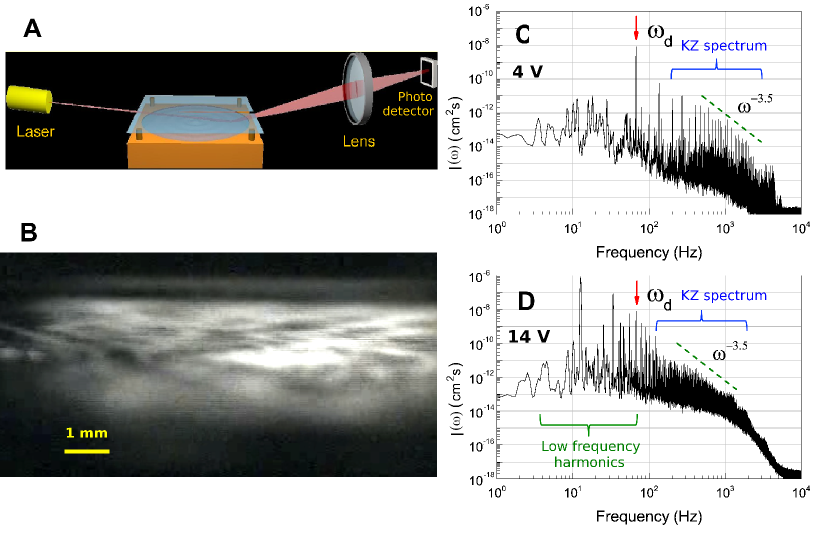
Figure 1: (A) Schematic of the experimental setup. Oscillations of the liquid helium surface are detected via variations of the total power of the reflected laser beam. An optical cryostat containing the cell is not shown. (B) Snapshot of the turbulent surface of superfluid helium taken through the cryostat windows in the reflected light. Large scale waves are clearly visible. The driving frequency is $\omega_{d}/2\pi=113$ Hz. A horizontal bar shows the length scale. (C,D) Formation of large-amplitude waves on the surface of superfluid helium at $\omega<\omega_{d}$ by increasing the AC driving voltage from $U_{d}=4$ V (c) to 14 V (B). The driving frequency (arrow) is $\omega_{d}/2\pi=68$ Hz. The wavelength at the driving frequency $\omega_{d}$ is $\simeq 780$ $\mu$m. The conventional direct Kolmogorov-Zakharov (KZ) spectrum of capillary turbulence $I({\omega})\propto\omega^{-3.5}$ between $2\times 10^{2}$ Hz $<\omega/2\pi<2\times 10^{3}$ Hz is shown by the dashed line in plates C and D. Formation of low-frequency harmonics at $\omega<\omega_{d}$ with amplitudes larger than those at the driving frequency $\omega_{d}$, in addition to KZ spectrum, are clearly visible for high-amplitude driving $U_{d}=14$ V in D.

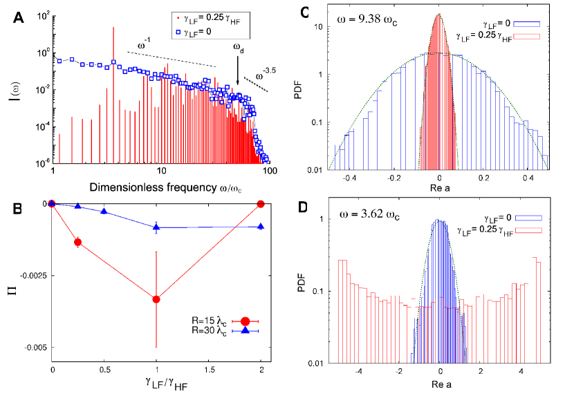
Figure 2: (A) Numerical steady-state spectrum $I(\omega)$ of sustained surface oscillations in the presence of low- and high-frequency damping (red peaks) and in the presence of only high-frequency damping (blue open squares). The spectrum is shown in units of $\lambda_{c}^{2}t_{c}$. The surface is driven at a frequency $\omega_{d}$ of the 50th resonance (arrowed). The high-frequency Kolmogorov-Zakharov spectrum $I(\omega)\propto\omega^{-3.5}$ is formed for $\omega>\omega_{d}$, as consistent with Fig. 1D. With the absence of low-frequency damping, $\gamma_{LF}=0$, the numerical wave spectrum (blue open squares) approaches the thermal-equilibrium spectrum $I({\omega})\propto\omega^{-1}$ that carries no energy flux. The power-law spectral behavior $I(\omega)\propto\omega^{-3.5}$ and $\omega^{-1}$ are shown by dashed lines. The curve connecting the squares is shown to guide the eye. The radius of the cylindrical cell is $R=15\lambda_{c}$; $\omega_{c}=(\rho g^{3}/\alpha)^{1/4}$ and $\lambda_{c}=(\alpha/\rho g)^{1/2}$ are used as units of frequency and length, respectively. (B) Energy flux ${\Pi}$ in units of $\alpha\omega_{c}$, incoming to the spectral domain $\omega<\omega_{d}$, that supports sustained low-frequency oscillations of the fluid surface, as a function of the low-frequency damping coefficient $\gamma_{LF}$. The simulations were performed for the cell radii $R=15\lambda_{c}$ (red circles) and $30\lambda_{c}$ (blue triangles). Vertical bars show the fluctuations of the flux as a standard deviation about the mean. The line segments connecting the points are shown to guide the eye. (C,D) Probability distribution functions of $Re(a)$ for the 20th resonant mode at frequency $\omega=9.38\omega_{c}$ (C) and for the 10th mode at frequency $\omega=3.62\omega_{c}$ (D) in the absence of low-frequency damping, $\gamma_{LF}=0$ (blue), and at $\gamma_{LF}=0.25\gamma_{HF}$ (red). PDFs are calculated for the spectra shown in A. Green lines show the Gaussian fit to the PDFs. It is seen in D that the Gaussian function fits the PDF for the 10th mode only if there is no low-frequency damping (blue bars). When the low-frequency dumping is applied and the bi-directional energy flux is thereby established, the PDF for the 10th mode (red bars in D) is far from Gaussian.

Supplementary Materials

1. Experimental techniques. The experimental arrangements were similar to those in our previous experiments with superfluid helium and liquid hydrogen [14]. The cup in which the helium was condensed has inner radius $R=30$ mm and depth $4$ mm. The experiments were conducted at temperature $T=1.7$ K of the superfluid liquid. The power $P(t)$ was measured with a photodetector and sampled with an analog-to-digital converter. The capillary-to-gravity wave transition on the surface of superfluid helium is at frequency $\sim 25$ Hz. The finite depth of the waves only influences the wave dispersion $\omega=\omega({k})$ at low frequencies $\omega<10$ Hz. The capillary wave length for superfluid helium is $\lambda_{c}=0.17$ cm. The kinematic viscosity of He-II at $T=1.7K$ is $\nu=2.6\times 10^{-4}$ cm²/s, which is $\sim 40$ times lower than that for water at $T=20$ C [19]. The measurements of wave damping in the cell showed that the quality factor at low frequencies $\omega<\omega_{d}$ is $Q\sim 10^{3}$.

2. Numerical Modeling. The deviation of the surface from the equilibrium flat state is expressed by time-dependent amplitudes $a_{k}(t)$ of the normal modes [10]. We assume angular symmetry of the surface, so its deviation for capillary waves is $\zeta(r,t)=\sum_{k}\sqrt{k/2\omega_{k}\rho AJ_{0}(\beta_{i})^{2}}$ $\times(a_{k}(t)+a_{k}^{*}(t))J_{0}(kr)$, where $r$ is the distance from the center of the cell, $J_{0}(x)$ is the Bessel function of the zero order, $A$ is the free-surface area, $\omega(k)$ is the linear dispersion relation given by Eq. 1, $k\equiv k_{n}=\beta_{n}/R$ is the radial wave number, $n>0$ is an integer index labeling the resonant radial modes, and $\beta_{n}$ is the $n$th zero of the first-order Bessel function $J_{1}(\beta_{n})=0$. In the simulations, $r$ is measured in units of the capillary length scale $\lambda_{c}$, and time $t$ is measured in the units of $t_{c}=\omega_{c}^{-1}$. The driving force is applied at a given radial mode $k_{d}$. Due to angular isotropy, we utilize the angle-averaged dynamical equation for $a_{k}(t)$ [11],

$${da_{k}(t)\over dt} = -i\sum_{k_{1},k_{2}}V_{k,k_{1},k_{2}}\,D_{k,k_{1},k_{2}}\,a_{k_{1}}(t)a_{k_{2}}(t)e^{i(\omega(k)-\omega({k_{1}})-\omega({k_{2}}))t}$$ (4)

$$- 2i\sum_{k_{1},k_{2}}V_{k_{1},k,k_{2}}^{*}\,D_{k_{1},k,k_{2}}\,a_{k_{1}}(t)a_{k_{2}}^{*}(t)e^{i(\omega(k)+\omega({k_{2}})-\omega({k_{1}}))t}-\gamma(\omega({k}))a_{\bm{k}}(t).$$

The coupling coefficients ${V}_{k,k_{1},k_{2}}$ characterize the interaction strengths between waves with wave numbers $k$, $k_{1}$, and $k_{2}$; instead of taking the exact value for capillary waves, we model it by ${V}_{k,k_{1},k_{2}}=\epsilon\sqrt{\omega(k)\omega({k_{1}})\omega({k_{2}})}$ [1]. Star denotes complex conjugate, $i$ stands for the imaginary unit, and $D_{k_{1},k,k_{2}}=1/2\pi\Delta(k,k_{1},k_{2})$, where $\Delta(k,k_{1},k_{2})$ is the area of the triangle with sides $k$, $k_{1}$, and $k_{2}$. We consider $n_{\rm max}=100$ radial modes. The dimensionless factor $\epsilon\ll 1$ characterizes nonlinearity of the system and is of the order of the maximum surface slope with respect to the horizontal [10]. We set $\epsilon=10^{-2}$ as a representative value [20]. Due to the small nonlinearity, we only retain three-wave interactions in Eq. 4; the inclusion of four-wave scattering requires special considerations [31] and is deferred to future studies.

Driving was at the 50th mode by fixing the wave amplitude $a_{d}\equiv|a_{k_{d}}(t)|$ at a given value, set in the present simulations as $(\lambda_{c}^{7/2}\omega_{c}\rho)^{-1/2}a_{d}=0.1$. We also add wave damping at both high and low frequencies, to mimic the physical effects that remove energy from the system. Specifically, we model the wave damping coefficient as

$$\gamma(\omega)=\gamma_{LF}(\omega)+\gamma_{HF}(\omega),$$ (5)

which is the sum of damping at low frequencies below the 10th resonance in the cell, with $\gamma_{LF}(\omega)=\gamma_{LF}g_{LF}(\omega)$, as well as damping at high frequencies above the 80th resonance, with $\gamma_{HF}(\omega)=\gamma_{HF}g_{HF}(\omega)$. The range of wave frequencies between the 10th and 80th resonant frequencies can be considered as a “numerical inertial interval” in which damping is absent. The dimensionless damping factor at high frequencies was set as $\gamma_{HF}=5\times 10^{-2}\omega_{c}$. Damping at high resonant numbers $n>n_{HF}=80$ is modeled as $g_{HF}(n)=(n-n_{HF})^{2}/(n_{\rm max}-n_{HF})^{2}$, and $g_{HF}(n)=0$ for $n\leq n_{HF}$. For model waves on a fluid layer of finite depth, we model damping at low resonant numbers $n<n_{LF}=10$ as $g_{LF}(n)=(n_{LF}-n)/n_{LF}$, and $g_{LF}(n)=0$ for $n\geq n_{LF}$. The low-frequency damping coefficient $\gamma_{LF}$ is varied between $0$ and $2\gamma_{HF}$. To calculate the dependence of $a_{k}(t)$ on time $t$, we integrated Eq. 4 until the system reached the steady state. We found numerical convergence and energy conservation with $10^{-7}$ numerical accuracy. The wave spectrum is calculated as the time-averaged quantity $N(k)=\langle|a_{k}(t)|^{2}\rangle$. For capillary waves, the time-averaged correlation function is $I(\omega)=N(k(\omega))$, where $N(k)$ is expressed as a function of the wave frequency $\omega$ via the relation $k=k(\omega)$ from Eq. 1 [20].

References and Notes

- [1] V. E. Zakharov, V. S. L’vov, G. Falkovich, Kolmogorov Spectra of Turbulence I (Springer, Berlin, 1992).
- [2] A. N. Kolmogorov, Doklady Akad. Nauk S.S.S.R. 30, 299 (1941).
- [3] R. G. Dean, Water Wave Kinetics, A. Torum, O. T. Gudmestad, eds. (Kluwer, Amsterdam, 1990), pp. 609–612.
- [4] L. M. Smith, Y. Lee, J. Fluid Mech. 535, 111 (2005).
- [5] D. J. Southwood, Nature 271, 309 (1978).
- [6] F. L. Scarf, D. A. Gurnett, W. S. Kurth, Nature 292, 747 (1981).
- [7] G. S. Bisnovatyi-Kogan, S. A. Silich, Rev. Mod. Phys. 67, 661 (1995).
- [8] Y. Toba, J. Ocean. Soc. Japan 29, 209 (1973).
- [9] U. Frisch, Turbulence (Cambridge University Press, Cambridge, 1995).
- [10] V. E. Zakharov, N. N. Filonenko, J. Appl. Mech. Tech. Phys. 8, 37 (1967).
- [11] A. N. Pushkarev, V. E. Zakharov, Phys. Rev. Lett. 76, 3320 (1996).
- [12] W. B. Wright, R. Budakian, D. J. Pine, S. J. Putterman, Science 278, 1609 (1997).
- [13] E. Henry, P. Alstrom, M. T. Levinsen, Europhys. Lett. 52, 27 (2000).
- [14] L. V. Abdurakhimov, M. Y. Brazhnikov, A. A. Levchenko, Low Temp. Phys. 35, 95 (2009).
- [15] L. Deike, M. Berhanu, E. Falcon, Phys. Rev. E 89, 023003 (2014).
- [16] A. J. Szeri, J. Fluid Mech. 332, 341 (1997).
- [17] H. Che, M. L. Goldstein, A. F. Viñas, Phys. Rev. Lett. 112, 061101 (2014).
- [18] I. M. Khalatnikov, An Introduction to the Theory of Superfluidity (Benjamin, New York, 1965).
- [19] L. V. Abdurakhimov, M. Y. Brazhnikov, I. A. Remizov, A. A. Levchenko, JETP Lett. 91, 271 (2010).
- [20] M. Brazhnikov, A. Levchenko, L. Mezhov-Deglin, Instrum. Exp. Tech. 45, 758 (2002).
- [21] M. Y. Brazhnikov, G. V. Kolmakov, A. A. Levchenko, L. P. Mezhov-Deglin, JETP Lett. 82, 565 (2005).
- [22] M. Shats, H. Punzmann, H. Xia, Phys. Rev. Lett. 104, 104503 (2010).
- [23] E. Falcon, C. Laroche, S. Fauve, Phys. Rev. Lett. 98, 094503 (2007).
- [24] R. Savelsberg, W. van de Water, Phys. Rev. Lett. 100, 034501 (2008).
- [25] B. Christiansen, P. Alstrom, M. T. Levinsen, J. Fluid Mech. 291, 323 (1995).
- [26] E. Balkovsky, G. Falkovich, V. Lebedev, I. Y. Shapiro, Phys. Rev. E 52, 4537 (1995).
- [27] S. Lukaschuk, S. Nazarenko, S. McLelland, P. Denissenko, Phys. Rev. Lett. 103, 044501 (2009).
- [28] E. Herbert, N. Mordant, E. Falcon, Phys. Rev. Lett. 105, 144502 (2010).
- [29] B. Miquel, A. Alexakis, C. Josserand, N. Mordant, Phys. Rev. Lett. 111, 054302 (2013).
- [30] A. N. Ganshin, V. B. Efimov, G. V. Kolmakov, L. P. Mezhov-Deglin, P. V. E. McClintock, Phys. Rev. Lett. 101, 065303 (2008).
- [31] G. During, C. Falcon, Phys. Rev. Lett. 103, 174503 (2009).
-
1.