Linear Hamilton Jacobi Bellman Equations in High Dimensions

Abstract

The Hamilton Jacobi Bellman Equation (HJB) provides the globally optimal solution to large classes of control problems. Unfortunately, this generality comes at a price, the calculation of such solutions is typically intractible for systems with more than moderate state space size due to the curse of dimensionality. This work combines recent results in the structure of the HJB, and its reduction to a linear Partial Differential Equation (PDE), with methods based on low rank tensor representations, known as a separated representations, to address the curse of dimensionality. The result is an algorithm to solve optimal control problems which scales linearly with the number of states in a system, and is applicable to systems that are nonlinear with stochastic forcing in finite-horizon, average cost, and first-exit settings. The method is demonstrated on inverted pendulum, VTOL aircraft, and quadcopter models, with system dimension two, six, and twelve respectively.

I Introduction

The Hamilton Jacobi Bellman (HJB) equation is central to control theory, yielding the optimal solution to general problems specified by known dynamics and a specified cost functional. Given the assumption of quadratic cost on the control input, it is well known that the HJB reduces to a particular Partial Differential Equation (PDE) [14]. While powerful, this reduction is not commonly used as the PDE is of second order, is nonlinear, and examples exist where the problem may not have a solution in a classical sense [11]. Furthermore, each state of the system appears as another dimension of the PDE, giving rise to the curse of dimensionality [5]. Since the number of degrees of freedom required to solve the optimal control problem grows exponentially with dimension, the problem becomes intractable for systems with all but modest dimension.

In the last decade researchers have found that under certain, fairly non-restrictive, structural assumptions, the HJB may be transformed into a linear PDE, see, e.g., [41] and [23], with an interesting analogue in the discretized domain of Markov Decision Processes (MDP) [40]. The implications for this discovery are numerous, and research has only begun to tap into the computational benefits [dvijotham2012linearly] and [21]. The work presented here is a continuation of this theme, and uses the linearity of this particular form of the HJB PDE to push the computational boundaries of the HJB.

Our method relies on recent work in Separated Representations (SR) [7], which have recently emerged as a method to solve a number of problems in machine learning and the numerical solution of PDEs with complexity that scales linearly with dimension, bypassing the curse of dimensionality. The central idea of this paper is to approximate the solution, and its associated operators, by a low rank tensor. If the problem’s components can be adequately modeled in this regime, then the complexity grows with the rank of the approximation, rather than the dimensionality. For many problems of interest this proves to be a valid modeling assumption.

II Related Work

We combine two previously disjoint threads of research. The first is the study of HJB equations, while the second is the study of high dimensional tensors and their approximations.

II-A Linearly Solvable Stochastic Optimal Control

The study of linearly solvable Stochastic Optimal Control (SOC) problems has developed along two lines of investigation. One is that of Linear MDPs [41], in which a control design problem may be solved via a linear set of equations given several structural assumptions. By taking the continuous limit of the discretization, a linear PDE is obtained. In another line of work begun by Kappen [23] the same linear PDE has been found through a particular transformation of the HJB. While the linearity of the HJB provides computational benefits in terms of the numerical techniques available, the curse of dimensionality prevents existing techniques from scaling to realistic problems of interest. This has been addressed through the use of the Path Integral techniques [38, 39], which rely on Monte Carlo techniques via the Feynman-Kac Lemma. The solution of the Linear PDE at an individual point in the state space is solved via an ensemble of Brownian motions. While these sampling techniques are formally independent of state space dimension, they may nonetheless be computationally expensive and typically only provide guarantees in the asymptotic regime. Furthermore, as the solution is only valid at an individual point, these solutions must be solved for all anticipated states that will occur over the course of a trajectory. These techniques have nonetheless shown notable success [36].

II-B Nonlinear Hamilton Jacobi Bellman Equations in Control

HJB equations have arisen as objects of study in the research of Control Lyapunov Functions. These functions generalize the notion of Lyapunov stability, allowing for the control signal to be incorporated in the analysis of a system’s stability [35]. These techniques may be seen as a relaxation of the conditions that lead to optimality for the HJB, and thus existing CLF-synthesis techniques are in general suboptimal. This may be ameliorated by combining CLFs with Euler-Lagrange equations which arise from the Pontraygin maximum principle, typically recognized as Model Predictive Control or Receding Horizon Control [34]. Indeed, many planning techniques may be understood as heuristic or approximate methods to solve the HJB [27, 20].

Ours is not the first study of numerical techniques to solve the HJB PDE directly. In [31] level-set algorithms are used to solve variants of the HJB that relate to the calculation of reachable sets. In [2], the authors uses high order Taylor expansions to approximate the HJB directly. McEaney [30] has developed another curse-of-dimensionality free method which relies on a max-plus expansion of the solution, with complexity that scales with the number of basis solutions, each requiring the solution to a Riccati system.

Lasserre provides an alternative framework to solve the HJB by constraining the moments of the solution, producing bounds on the moments that can be made to converge through a hierarchy of optimization problems [26, 25]. These techniques seek to reduce the fundamental infinite dimensional linear program to a semidefinite program with a finite number of degrees of freedom by truncating the solution moments. This is currently an active and growing area of research [29]. A similar construction of Lasserre hierarchies was proposed in [21] using Sum of Squares techniques, producing upper and lower bounds to the linear HJB. However, all fall prey to the curse of dimensionality, save the work of McEaney, and in practice are limited to dimensions of five or lower. We argue that while the techniques presented herein do not yet apply to all optimal control problems at the moment, they apply to a broad class of systems, with astounding computational gains. We discuss how these techniques may in fact be applied without these assumptions in our concluding discussion.

Researchers have previously attacked the intractability of the HJB through discretization of the system state space, creating an MDP. The curse of dimensionality is mitigated in this context by parameterizing the value function with a sparse set of basis, giving rise to Approximate Dynamic Programming, or when the basis may change online Adaptive Dynamic Programming (ADP) [6]. These techniques have constraint sets that formally grow exponentially with dimensionality [12]. Nonetheless, these techniques are the most popular method to deal with the curse of dimensionality, and have even been used to surpass human capabilities on complex time dependent games via synthesis with modern machine learning techniques [32]. These methods are closest to ours in spirit, and our method could be seen as generating a sparse basis, as is desired in ADP, albeit ours is performed without recourse to an MDP, with the attendant constraints.

II-C High Dimensional Tensors

Tensor approximations have historically been developed with the goal of approximating high dimensional data, yielding rise to the framework used here under the names CANDECOMP/PARAFAC [17, 9]. However, [7] demonstrated that these approximation techniques were applicable to the linear systems describing discretized PDEs. This technique has been applied in several domains, including computational chemistry and quantum physics, among others [24]. In particular, [37] examines their use in the context of stationary Fokker-Planck equations. There are interesting connections between the fundamental task of these techniques, approximating a tensor with one of lower rank, and convex relaxation based methods [10, 15]. Unfortunately, low rank tensor approximation is NP-hard in general, and an optimal solution is not to be expected [18].

III The Linear Hamilton Jacobi Bellman Equation

We begin by constructing the value function, which captures the cost-to-go from a given state. If such a quantity is known, the optimal action may be chosen as that which follows the gradient of the value, bringing the agent into the states with highest value over the remaining time horizon. We define $x_{t}\in\mathbb{R}^{n}$ as the system state at time $t$, control input $u_{t}\in\mathbb{R}^{m}$ , and dynamics that evolve according to the equation

$$dx_{t}=\left(f\left(x_{t}\right)+G\left(x_{t}\right)u_{t}\right)dt+B\left(x_{t}\right)d\omega_{t}$$ (1)

on a compact domain $\Omega$, and where the expressions $f(x)$, $G(x)$, $B(x)$ are assumed to be smoothly differentiable, but possibly nonlinear, functions, and $\omega_{t}$ is Gaussian noise with covariance $\Sigma_{\epsilon}$. The system has cost $r_{t}$ accrued at time $t$ according to

$$r\left(x_{t},u_{t}\right)=q\left(x_{t}\right)+\frac{1}{2}u_{t}^{T}Ru_{t}$$ (2)

where $q(x)$ is a state dependent cost. We require $q(x)\geq 0$ for all $x$ in the problem domain and $R$ positive definite. The goal is to minimize the expectation of the cost functional

$$J(x,u)=\phi_{T}\left(x_{T}\right)+\int_{0}^{T}r\left(x_{t},u_{t}\right)dt$$ (3)

where $\phi_{T}$ represents a state-dependent terminal cost. The solution to this minimization is known as the value function, where, beginning from an initial point $x_{0}$ at time $0$

$$V\left(x_{0}\right)=\min_{u_{[0,T]}}\mathbb{E}\left[J\left(x_{0}\right)\right]$$ (4)

where we use the shortand $u_{[t,T]}$ to denote the trajectory of $u_{t}$ over the time interval $t\in[t,T]$, and the expectation is taken over a realizations of the trajectory $x_{\left[0,T\right]}$ with initial condition $x_{0}$.

The associated Hamilton-Jacobi-Bellman equation, arising from Dynamic Programming arguments [14], is

$$-\partial_{t}V=\min_{u}\left(r+\left(\nabla_{x}V\right)^{T}f+\frac{1}{2}Tr\left(\left(\nabla_{xx}V\right)G\Sigma_{\epsilon}G^{T}\right)\right).$$ (5)

As the control effort enters quadratically into the cost function it is a simple matter to solve for it analytically by substituting (2) into (5) and finding the minimum, yielding:

$$u^{*}=-R^{-1}G^{T}\left(\nabla_{x}V\right).$$ (6)

The minimal control, $u^{*}$, may then be substituted into (5) to yield the following nonlinear, second order partial differential equation

$$\begin{split}-\partial_{t}V&=q+\left(\nabla_{x}V\right)^{T}f-\frac{1}{2}\left(\nabla_{x}V\right)^{T}GR^{-1}G^{T}\left(\nabla_{x}V\right)\\ &\phantom{=}+\frac{1}{2}Tr\left(\left(\nabla_{xx}V\right)B\Sigma_{\epsilon}B^{T}\right).\end{split}$$ (7)

The difficulty of solving this PDE is what usually prevents the value function from being directly solved for. However, it has recently been found [23, 41] that with the assumption that there exists a $\lambda\in\mathbb{R}$ and a control penalty cost $R\in\mathbb{R}^{n\times n}$ satisfying this equation

$$\lambda G(x)R^{-1}G(x)^{T}=B(x)\Sigma_{\epsilon}B(x)^{T}\triangleq\Sigma_{t}$$ (8)

and using the logarithmic transformation, with $\lambda>0$,

$$V=-\lambda\log\Psi$$ (9)

it is possible, after substitution and simplification, to obtain the following linear PDE from Equation (7)

$$-\partial_{t}\Psi=-\frac{1}{\lambda}q\Psi+f^{T}\left(\nabla_{x}\Psi\right)+\frac{1}{2}Tr\left(\left(\nabla_{xx}\Psi\right)\Sigma_{t}\right).$$ (10)

This transformation of the value function, which we call here the desirability [41], provides an additional, computationally appealing, method by which to calculate the value function.

Remark 1.

The condition (8) can roughly be interpreted as a controllability-type condition: the system controls must span (or counterbalance) the effects of input noise on the system dynamics. A degree of designer input is also given up, as the constraint restricts the design of the control penalty R, requiring that control effort be highly penalized in subspaces with little noise, and lightly penalized in those with high noise. Additional discussion may be found in [41].

The boundary conditions of (10) correspond to the exit conditions of the optimal control problem. This may correspond to colliding with an obstacle or goal region, and in the finite horizon problem there is the added boundary condition of the terminal cost at $t=T$. These final costs must then be transformed according to (9), producing added boundary conditions to (10).

Linearly solvable optimal control is not limited to the finite horizon setting. Similar analysis can be performed to obtain linear HJB PDEs for infinite horizon average cost, and first-exit settings, with the corresponding cost functionals and PDEs shown in Table I.

TABLE I: Linear Desirability PDE for Various Stochastic Optimal Control Settings. $L(\Psi):=f^{T}\left(\nabla_{x}\Psi\right)+\frac{1}{2}Tr\left(\left(\nabla_{xx}\Psi\right)\Sigma_{t}\right)$

	Cost Functional	Desirability PDE
Finite	$\phi_{T}(x_{T})+\int_{0}^{T}r(x_{t},u_{t})dt$	$\frac{1}{\lambda}q\Psi-\frac{\partial\Psi}{\partial t}=L(\Psi)$
First-Exit	$\phi_{T_{*}}(x_{T_{*}})+\int_{0}^{T}r(x_{t},u_{t})dt$	$\frac{1}{\lambda}q\Psi=L(\Psi)$
Average	$\lim_{T\to\infty}\frac{1}{T}\mathbb{E}\left[\int_{0}^{T}r(x_{t},u_{t})dt\right]$	$\frac{1}{\lambda}q\Psi-c\Psi=L(\Psi)$

IV Separated Representations of Tensors

Traditional numerical techniques to solve PDEs rely on the discretization of the domain. However, in these schemes the degrees of freedom in the problem grows exponentially with the number of dimensions. While tractable when the number of dimensions is small, in higher dimensions these problems become computationally prohibitive. In [7], Beylkin and Mohlenkamp proposed to model the solutions to such problems via so-called separated representations, which may be viewed as an extension of the separation of variables technique. Problem data, and the solution, is modeled as a sum of terms, each of which is dependent on individual dimensional variables. Specifically, a function is modeled as

$$f\left(x_{1},\ldots,x_{d}\right)\approx\sum_{l=1}^{r}s_{l}\phi_{1}^{l}(x_{1})\cdots\phi_{d}^{l}(x_{d}).$$ (11)

The key is that such a representation separates the dependence of the solution into each component dimension. By then framing operations to act on single dimensions, it is possible to create algorithms that need only operate along each dimension independently and thus scale linearly in $d$.

However, the complexity of the problem now grows with $r,$ denoted the separation rank. Thus, maintaining a low separation rank becomes paramount for any practical algorithm. Unfortunately, many operations inherently increase the separation rank, including vector addition and matrix-vector multiplication. This unbounded growth is mitigated by reducing the separation rank at each step of an algorithm in an attempt to continually maintain low rank approximations. Unfortunately, there are often no guarantees that a given function, or solution to a PDE, will have low separation rank and situations may arise where it is impossible to lower the rank while maintaining the desired accuracy.

Here we simply provide an introduction to the concept of a separated representation and discuss them in a manner tailored to our use. As such, we direct the reader to [7] for a complete treatment.

A vector $F$ in dimension $d$ is a discrete representation of a function $f$ on a rectangular domain, $\boldsymbol{F}=F(j_{1},\ldots,j_{d})$ where $j_{i}=1,\ldots,M_{i}$ are the indices along each dimension. A linear operator $\mathcal{A}$ in dimension $d$ is a linear map $\mathcal{A}:S\to S$ where $S$ is the space of functions in dimension $d$. A matrix $\mathbb{A}$ in dimension $d$ is a discrete representation of a linear operator in dimension $d.$

Definition 2.

For a given $\epsilon,$ we represent a vector $\boldsymbol{F}=F(j_{1},j_{2},\ldots,j_{d})$ in dimension $d$ as

$$\boldsymbol{F}\approx\sum_{l=1}^{r_{\textbf{F}}}s_{l}\bigotimes_{i=1}^{d}\boldsymbol{F}_{i}^{l}$$

where $\bigotimes$ denotes the tensor product and $\boldsymbol{F}_{i}^{l}$ are traditional vectors in $\mathbb{R}^{M_{i}}$ with entries $F_{i}^{l}(j_{i})$ and unit norm. For this to be an $\epsilon$ accurate representation we require that

$$\left\|\boldsymbol{F}-\sum_{l=1}^{r_{\textbf{F}}}s_{l}\bigotimes_{i=1}^{d}\boldsymbol{F}_{i}^{l}\right\|\leq\epsilon.$$

The integer $r$ is known as the separation rank.

The matrix definition is analogous, with the matrices ${\mathbb{A}_{i}^{l}\in\mathbb{R}^{M_{i}\times M_{i}}}$ in lieu of $\boldsymbol{F}_{i}^{l}=F_{i}^{l}(j_{i})$. Matrix multiplication is then performed as

$$\mathbb{A}F=\sum_{m=1}^{r_{\mathbb{A}}}\sum_{l=1}^{r_{F}}s_{m}^{\mathbb{A}}s_{l}^{F}\left(\mathbb{A}_{1}^{m}F_{1}^{l}\right)\otimes\cdots\otimes\mathbb{A}_{d}^{m}F_{d}^{l}.$$ (12)

Since matrix operations in this formulation reduce to individual operations along each dimension, as the dimensionality of the problem increases the complexity of these operations scales linearly, e.g., if we let $M_{i}$ = $M$ for all $i$ a matrix vector multiplication costs $O(r_{A}r_{F}dM^{2})$.

IV-A Alternating Least Squares

Any scheme that uses these separated representations will become computationally prohibitive if the separation ranks are allowed to grow unchecked. For example, in the matrix vector multiplication the separation rank of the output grows by a factor of $r_{A}r_{F},$ so even performing the most basic of operations may have a large impact on the separation rank. It is therefore necessary to periodically find lower rank approximations to various operators and vectors. If the assumption is that the discrete versions of the functions being represented have low separation rank, then any increase in the separation rank is only an artifact of the way operations are performed in these tensor representations, and we expect is possible to produce an accurate representation of the resultant tensor that has a reduced separation rank.

We provide a high level overview of the alternating least squares (ALS) algorithm, with the reader directed to [7] for details. This algorithm allows us to look for separated representations with lower separation rank and solve systems. A recently proposed variant relying on a randomized interpolative decomposition is presented in [8] and may be used as a precursor to ALS.

Given a vector with separated representation G, and an operator $\mathbb{A}$, ALS tries to either minimize $\left\|\textbf{F}-\textbf{G}\right\|$ or, with slight modification, $\left\|\mathbb{A}\textbf{F}-\textbf{G}\right\|$ subject to F having fixed rank $r_{F}.$ The algorithm sweeps through the coordinate directions, effectively performing block-gradient descent. For a fixed separation rank of F this process may be repeated until the algorithm has either achieved the desired accuracy, or has stagnated. If the algorithm has stagnated, and the representation error is not small enough, e.g., $\left\|\mathbb{A}\textbf{F}-\textbf{G}\right\|\geq\epsilon,$ a random rank-one tensor is added to F, and the ALS routine continues.

At an individual step in this iterative algorithm, all dimensions of the tensor F are held constant save one dimension $k,$ in which case the least-squares problem becomes linear in $\textbf{F}_{k}^{l}$ for $l=1,\ldots,r_{G}$. The resulting least squares problem is solved via derivation of the normal equations, yielding a linear set of equations. These were originally given in [7], but have been rederived in [37] in a more compact format as

$$\left(\begin{array}[]{ccc}M_{1,1}&\cdots&M_{1,r_{G}}\\ \vdots&\ddots&\vdots\\ M_{r_{G},1}&\cdots&M_{r_{G},r_{G}}\end{array}\right)\left(\begin{array}[]{c}F_{k}^{1}\\ \vdots\\ F_{k}^{r_{G}}\end{array}\right)=\left(\begin{array}[]{c}N_{1}\\ \vdots\\ N_{r_{G}}\end{array}\right)$$ (13)

where the components of the normal equations are given by

$$M_{i,j}=\sum_{i_{A}=1}^{r_{\mathbb{A}}}\sum_{j_{A}=1}^{r_{\mathbb{A}}}\left(A_{k}^{j_{A}}\right)^{T}A_{k}^{i_{A}}\prod_{d\neq k}\left\langle A_{d}^{i_{A}}F_{d}^{j},A_{d}^{j_{A}}F_{d}^{i}\right\rangle$$ (14)

$$N_{i}=\sum_{i_{A}=1}^{r_{\mathbb{A}}}\sum_{i_{G}=1}^{r_{G}}\left(A_{k}^{i_{A}}\right)^{T}G_{k}^{i_{G}}\prod_{d\neq k}\left\langle A_{d}^{i_{A}}F_{d}^{i},G_{d}^{i_{G}}\right\rangle$$ (15)

with the solution vector $\textbf{F}=\sum_{i=1}^{r_{\textbf{F}}}\otimes_{d=1}^{n}F_{d}^{i}$, the vector $\textbf{G}=\sum_{i=1}^{r_{\textbf{G}}}\otimes_{d=1}^{n}G_{d}^{i}$, and the operator $\mathbb{A}=\sum_{i=1}^{r_{\mathbb{A}}}\otimes_{d=1}^{n}A_{d}^{i}$, for $n$ the dimension of the system. When the operator $\mathbb{A}$ is the identity, the problem $\left\|\textbf{F}-\textbf{G}\right\|$ has additional structure that may be leveraged [7]. The solution to these linear equations provides a new F, with different components in the $k$ dimension, that has a smaller residual error. The algorithm continues by optimizing the components in the next, $k+1,$ dimension.

While the core ALS algorithm, with the identity operator, costs $\mathcal{O}\left(dM+dr_{\mathbf{F}}^{3}\right)$ per iteration, its use to solve a linear system costs $\mathcal{O}\left(dM^{3}+r_{\mathbb{A}}^{3}M^{3}\right)$ per iteration, where $d$ is the underlying dimensionality of the system, $M$ is the maximal number of mesh nodes along each dimension, and $r_{\mathbb{A}},(r_{\mathbf{F}})$ is the rank of the operator $\mathbb{A}$ (vector $\mathbf{F}$). See [7] for a more comprehensive list of algorithms that may be used with operators and vectors in separated representations.

V Separated Solution to the HJB

We make the modeling assumption that the problem data of (1) can be accurately represented, or approximated, with a low rank separated representation.

$$f_{i}(t,x)=\sum_{l=1}^{r_{f_{i}}}\bigotimes_{k=1}^{d}\left(f_{i}\right)_{d}^{l}$$ (16)

where $r_{f_{i}}$ is assumed to be small.

There is then the need to approximate the relevant operators present in (1), specifically the gradient and Hessian, in a low rank representation. A number of options exist, with varying levels of complexity in the analysis and accuracy, ranging from simple finite difference schemes to spectral differentiation techniques [43]. Specifically, the gradient along dimension $k$ is simply

$$\nabla_{k}=I_{1}\otimes\cdots\otimes I_{k-1}\otimes\nabla\otimes I_{k+1}\otimes\cdots\otimes I_{d}$$

while the Hessian has entries $\nabla_{k,j}=\nabla_{k}\cdot\nabla_{j}$, and the estimates of the derivative along an individual coordinate are simply a suitably high order finite difference scheme in one dimension. Thus, the directional gradient and second order terms may simply be constructed out of rank one representations. For example, using of sums of these rank one terms yields a representation for the Laplacian that has separation rank $d.$ However, such a representation may be not have minimal separation rank for a given accuracy. Other constructions specifically targeting the separated representation exist [7], for example a Laplacian approximation may be made with separation rank two, rather than requiring a full rank-$d$ sum of second order terms. Choices about how to approximate the operators may lead to some variation in the separation rank of the solutions since different strategies introduce different types of discretization error.

V-A Separation Rank of the HJB

Determining the separation rank of the HJB operator is straightforward. Denote the rank of a vector or operator $X$ as $r_{X}$. Recalling (10) and neglecting the time dependent component, the operator consists of three additive terms. The state-cost term $q\Psi$ is a diagonal operator along each dimension, and thus contributes $r_{q}$. The second, advection term is an inner product between the dynamics $f$ and the gradient, resulting in the multiplication of each element $f_{i}$ by a rank one operator, and then their summation. The contribution from this component results in separation rank $\sum_{k=1}^{d}r_{f_{i}}$. Finally, the second-order term requires the construction of $\Sigma_{t}$ in (8). Here the growth in the separation rank may be significant, due to the multiplicative contribution of $G$. However, given diagonal cost matrix $R$ or noise covariance $\Sigma_{\epsilon}$ the number of terms may collapse significantly. The separation rank of the HJB operator is simply the sum of these three terms’ rank.

The result is that the separation rank for individual problems may vary over a wide range, depending on the problem data. However, in many problems of interest it remains low. For even apparently complex systems, complexity typically manifests as nonlinear multiplicative terms in the dynamics. This form of complexity effectively adds no cost in terms of separation rank, and it is instead the number of additive terms that are of concern, which is typically small. Furthermore, in many applications the control and noise matrices typically contain constant terms, corresponding to tensors of separation rank one. Finally, for systems where a high separation rank accumulates, it remains possible to search for low rank structure by performing ALS on the operator before attempting to solve the linear system.

V-B Representation of Interior Boundary Conditions

Optimal control applications impose irregular boundary conditions on many problems of interest. For example, stabilization to the origin corresponds to a zero-cost point-boundary at the origin. Obstacles, or sub-task goals in temporal problems ([13], [22]), become boundary conditions as well, i.e. a set of Dirichlet boundary conditions within the domain.

We impose essential boundary conditions by setting the value of nodes to some desired value via linear equalities within the domain. Although in other settings it is desirable to remove the degrees of freedom from within the boundaries to save computational effort, in our context maintaining the grid form is a far greater concern. Specifically, we impose Dirichlet boundary conditions only on regions composed of hyper-cubes in the domain, allowing us to modify the domain with only a modest increase in the separation rank of the operator. We first eliminate the operators effect on this hypercube of the domain via a single subtraction, and then replace it with the identity operator via a single addition. The resulting operator $\bar{\mathbb{A}}$ with the desired boundary conditions has rank $r_{\bar{\mathbb{A}}}=d+2r_{\mathbb{A}}$.

VI Implementation Details and Examples

In the following examples, we approximate first and second order derivatives using eighth order finite differences, with the number of mesh points along each dimension varying between $n_{g}=100$ and $n_{g}=201$. The result are tensors that would typically not fit in the memory of even the largest modern super computers if expressed naively without the use of the separated representation. In each case we modeled the problem as first-exit (see Table I). In all cases the noise was assumed to enter the dynamics in the same manner as the control, with $G(x)=B(x)$ in (1).

The operator is constructed as described in Section V. The operator and boundary conditions are compressed independently using Alternating Least Squares with the linear system set to identity. With this low-rank representation, the problem is then solved using Alternating Least Squares for the HJB system. We employed the Matlab Tensor Toolbox [4, 1], for storage and manipulation of tensor objects.

The problems were solved on a quad-core 2.3Ghz i7-equipped laptop. We denote $\bar{u}$, $\bar{x}$ as the vector of system control inputs and states for each example.

VI-A Inverted Pendulum

In [33] the geometry of optimal control for the inverted pendulum on a cart was investigated in detail. In particular, they produce the value function for the inverted pendulum when actuated directly at the base

$$\dot{x}_{1} = x_{2}$$ (17)

$$\dot{x}_{2} = \frac{\frac{g}{l}\sin(x_{1})-\frac{1}{2}m_{r}x_{2}^{2}\sin(2x_{1})-\frac{m_{r}}{ml}\cos(x_{1})u}{\frac{4}{3}-m_{r}\cos^{2}(x_{1})}$$

and the cost function is $q(x)=0.1x_{1}^{2}+0.05x_{2}^{2}+0.01u^{2}$. This problem has periodic boundary conditions along the $x_{1}$ dimension, and we placed a Dirichlet boundary condition of $\phi(x_{1},\pm 11)=10$, i.e. a high penalty for exceeding the maximal angular velocity of $\dot{\theta}>11$ rad/s. An exit interior boundary was placed at the origin, with Dirichlet boundary conditions corresponding to unity desirability. We chose $n_{g}=201$ discretization points in each dimension.

The value function obtained by inverting the transformation (9) to the solution is shown in Figure 1. The process took approximately ten minutes, achieving error $e=5.22\cdot 10^{-5}$ with a basis of $r_{\Psi}=20$ rank one tensors. The five principal basis functions along each dimension are shown in Figure 2.

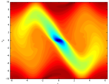
Figure 1: Cost to go for the inverted pendulum. The effects of the noise may be seen in the smoothing of the value function, in comparison to the deterministic case seen in [33].

$x_{1}$
$x_{2}$

Figure 2: Five principal basis functions for the inverted pendulum along the $x_{1}$, $x_{2}$ dimensions.

VI-B VTOL Aircraft

Next, we consider a Vertical Takeoff and Landing aircraft (also known as the Harrier Jet). We examine a planar cross section of the translational state, that is the jet’s $(x,y)$ location where $y$ is in the vertical direction. The system is characterized by second order dynamics with gravitational drift and trigonometric inputs, giving rise to a sixth dimensional nonlinear system. Specifically, the equations governing the system are given in [19] as

$$\ddot{x} = -u\sin(\theta)+\epsilon\,\tau\cos(\theta)$$

$$\ddot{y} = u\cos(\theta)+\epsilon\,\tau\sin(\theta)-g$$

$$\ddot{\theta} = \tau,$$

where $\epsilon=0.01$ in our example. The cost function chosen was $r=u^{2}$, and $q(x,y,\theta,\ldots)=1.0$ on the domain $x\in[-4,4],y\in[0,2],\dot{x}\in[-8,8],\dot{y}\in[-1,1],\dot{\theta}\in[-5,5]$, with $\theta$ periodic on $[-\pi,\pi]$. All boundaries were set to have boundary conditions $\Psi\mid_{\partial\Omega}=0$, save $y=0$, which had condition $\Psi\mid\partial\Omega=1-s^{2}$ for each coordinate direction $s$, placing a target of landing with zero velocities. Discretization $n_{g}=100$ were used along each dimension. We limited the solver to twenty iterations, which required approximately five minutes. We omit the resulting basis functions due to space restrictions. We also show the error and basis function weighting in Figure 4. A sample trajectory when executing the policy in closed loop in Figure 3.

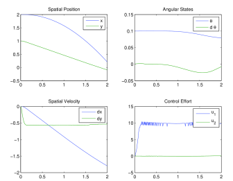
Figure 3: Sample trajectory when executing desirability for the VTOL aircraft.

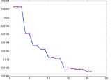
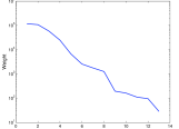
Figure 4: Convergence and weighting for the VTOL solution. The red markers indicate at which iterations the ALS algorithm enriched the solution by adding a basis element.

VI-C Quadcopter

The next example is in the stabilization of a quadcopter. The derivation of the dynamics may be found in [16], and results in a system of order twelve with highly nonlinear dynamics.

$$m\ddot{x} = u\left(\sin\phi\sin\psi+\cos\phi\cos\psi\sin\theta\right)$$

$$m\ddot{y} = u\left(\cos\phi\sin\theta\sin\psi-\cos\psi\sin\phi\right)$$

$$m\ddot{z} = u\cos\theta\cos\phi-mg$$

$$\ddot{\psi} = \tilde{\tau}_{\psi}$$

$$\ddot{\theta} = \tilde{\tau}_{\theta}$$

$$\ddot{\phi} = \tilde{\tau}_{\phi}$$

where $\eta=\left(x,y,z\right)$ are in the horizontal and vertical plane, respectively, while $\tilde{\tau}=\left(\tilde{\tau}_{\psi},\tilde{\tau}_{\theta},\tilde{\tau}_{\phi}\right)$ are the yaw, pitch, and roll moments. For simplicity, we assume we have direct actuation control over $\tilde{\tau}$. We solve the problem with $r=\|\bar{u}\|$ and $q(\bar{x})=2$. Similar to the VTOL example, we penalize all boundaries, save $x=1$, where a quadratic along the boundary in each dimension induces the system to exit with small velocity in all dimensions. Discretization $n_{g}=100$ was again used along each dimension.

In this instance $f(x)\equiv 0$ for all but the $z-$acceleration, which has separation rank one, and $G(x)$ has separation rank two for only the first three coordinate dimensions. Due to the matching condition (8), we model noise as entering the system as entering the same subspace as the control input, with $B(x)\triangleq G(x)$. The formation of the partial differential operator requires $r_{\mathbb{A}}=56$, but the ALS algorithm is able to compress this to $r_{\tilde{\mathbb{A}}}=24$ with a relative error of $10^{-4}$ in approximately two minutes, indicating there exist a great deal of underlying structure that the system is able to exploit.

Only five basis functions were computed, with the results shown in Figure 5. The time for each ALS iteration is shown in Figure 6, along with the weighting upon each basis function. The total computation time was approximately ten minutes. Finally, Figure 7 shows a trajectory of the closed loop system.

Figure 5: Complete basis function set for Quadcopter policy.

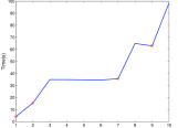
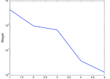
Figure 6: Convergence and weighting for the quadcopter solution.

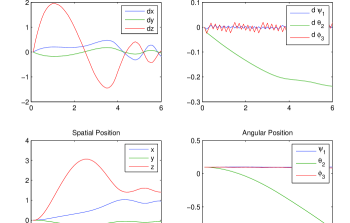
Figure 7: Simulation of the closed loop quadcopter system.

VII Discussion

There are a number of immediate implications of this work. The first is in the control of nonlinear distributed systems. In these problems, additional systems manifest as additional dimensions for the PDE. Formally, the complexity therefore grows linearly with the number of sub-systems. As well, if the coupling between such subsystems is sparse, it is expected that this interconnection could be simply described, leading to low separation rank necessary to describe the coupled dynamics.

The techniques that have been developed which rely on Sums of Squares programming [21] have been limited in degree and dimensionality due to the factorial growth in monomial basis. However, returning to the development of the separated representation, each rank-1 term corresponds to a single monomial. By limiting the basis to those with high representative power, such problems may be scaled to arbitrarily high degree and dimensionality.

A key limitation of this work is that it requires the structural assumptions of (8) to obtain a linear set of equations for which ALS may be applied. The general nonlinear value function may not be directly solved. However, it has been shown that iterative linearization of the nonlinear equations may be constructed in such a manner as to solve the more general HJB problem without our structural assumptions [28].

As alluded to in the introduction, these linear PDEs have a discrete counterpart in linearly solvable MDPs [41, 40]. In general, MDPs must be solved through an iterative maximization process known as value or policy iteration. However, by assuming a similar restriction on the noise of the system, specifically that it enters into the system along the same transitions actuated by the control input, Todorov has demonstrated that average cost, first exit, and finite horizon optimal control problems may be solved through a set of linear equations. It remains to be seen if the separated representation approach may also be adapted for linear MDPs.

VII-A Applications of the Hamilton Jacobi Bellman Solution

The Hamilton Jacobi Bellman equation yields the optimal solution to a general form of control problem, and its impact is present in many components of control theory. Of course, the most straightforward application is that emphasized in the previous development, that of trajectory generation. The most likely trajectory of the system is in fact related to the desirability, and can be calculated from the HJB solution [42]. Furthermore, although the HJB solution provides optimal trajectories, by (6) the method also provides an optimal feedback controller. The result is an architecture that is both robust and far-sighted, with the feedback controller and planner both accounting for the other. This controller has several appealing properties. In contrast to MPC-based schemes, no online computation is required, and can be seen as the optimal, continuous limit of gain scheduling.

The ability to solve these problems for arbitrary dimension, this opens a new synthesis technique for a number of difficult problems. The first of these is the generation of Control Lyapunov Functions, which may be done by placing an exit with zero cost at the origin for the first-exit problem. The benefits of such automatic generation techniques may be seen in works such as [3], where significant effort goes towards generating CLFs for particular applications, and further effort is used towards bringing these CLFs towards optimality.

Conclusion

In this work a method to solve the Hamilton Jacobi Bellman equation for nonlinear, stochastic systems with complexity the scales linearly with dimension has been proposed. Although several structural assumptions are required, systems that do not meet these may be approximated by the introduction of noise and control effort with arbitrary magnitudes. The implications are vast, as the curse of dimensionality no longer necessarily prevents the use of optimal control on complex, realistic systems. As the Hamilton Jacobi Bellman equations touch every aspect of control theory, the techniques here hold promise in a wide variety of topics. In particular, there are a number of important linear PDEs in control theory and estimation, including the Fokker Planck, Duncan-Mortensen-Zakai, and other equations. With the methods presented here, recourse to linearization techniques for these problems is no longer the only possibility.

References

- [1] E. Acar, D. M. Dunlavy, and T. G. Kolda. A scalable optimization approach for fitting canonical tensor decompositions. Journal of Chemometrics, 25(2):67–86, February 2011.
- [2] C. O. Aguilar and A. J. Krener. Numerical solutions to the bellman equation of optimal control. Journal of optimization theory and applications, 160(2):527–552, 2014.
- [3] A. Ames, K. Galloway, J. W. Grizzle, and K. Sreenath. Rapidly Exponentially Stabilizing Control Lyapunov Functions and Hybrid Zero Dynamics. IEEE Transactions on Automatic Control, (99):1, 2014.
- [4] B. W. Bader, T. G. Kolda, et al. Matlab tensor toolbox version 2.5. Available online, January 2012. http://www.sandia.gov/ tgkolda/TensorToolbox/.
- [5] R. E. Bellman and S. E. Dreyfus. Applied Dynamic Programming. Princeton University Press.
- [6] D. P. Bertsekas. Dynamic Programming and Optimal Control, volume 2. Athena Scientific, 4 edition, Mar. 2012.
- [7] G. Beylkin and M. J. Mohlenkamp. Algorithms for Numerical Analysis in High Dimensions. SIAM Journal on Scientific Computing, 26(6):2133–2159, Jan. 2005.
- [8] D. J. Biagioni, D. J. Beylkin, and G. Beylkin. On Rank Reduction of Separated Representations. arXiv.org:1306.5013v1, June 2013.
- [9] J. D. Carroll and J.-J. Chang. Analysis of individual differences in multidimensional scaling via an n-way generalization of “Eckart-Young” decomposition. Psychometrika, 35(3):283–319, Sept. 1970.
- [10] V. Chandrasekaran, B. Recht, P. A. Parrilo, and A. S. Willsky. The Convex Geometry of Linear Inverse Problems. Foundations of Computational Mathematics, 12(6):805–849, Oct. 2012.
- [11] M. G. Crandall, H. Ishii, and P.-L. Lions. User’s guide to viscosity solutions of second order partial differential equations. arXiv.org:math/9207212v1, June 1992.
- [12] D. P. de Farias and B. Van Roy. The linear programming approach to approximate dynamic programming. Operations Research, 51(6):850–865, 2003.
- [13] P. M. Esfahani, D. Chatterjee, and J. Lygeros. Motion Planning via Optimal Control for Stochastic Processes. arXiv.org:1211.1138v1, Nov. 2012.
- [14] W. H. Fleming and H. M. Soner. Controlled Markov Processes and Viscosity Solutions. Springer, 2 edition, Mar. 2006.
- [15] S. Gandy, B. Recht, and I. Yamada. Tensor completion and low-n-rank tensor recovery via convex optimization. Inverse Problems, 27(2):025010, Jan. 2011.
- [16] L. R. García Carrillo, A. E. Dzul López, R. Lozano, and C. Pégard. Modeling the quad-rotor mini-rotorcraft. Quad Rotorcraft Control, pages 23–34, 2013.
- [17] R. A. Harshman. Foundations of the PARAFAC procedure: Models and conditions for an" explanatory" multimodal factor analysis. Working Papers in Phonetics, 1970.
- [18] J. Håstad. Tensor rank is NP-complete. Journal of Algorithms, 11(4):644–654, 1990.
- [19] J. Hauser, S. Sastry, and G. Meyer. Nonlinear control design for slightly non-minimum phase systems: application to V/STOL aircraft. Automatica, 28(4):665–679, 1992.
- [20] M. B. Horowitz and J. W. Burdick. Optimal navigation functions for nonlinear stochastic systems. Intelligent Robots and Systems (IROS), 2014.
- [21] M. B. Horowitz and J. W. Burdick. Semidefinite relaxations for stochastic optimal control policies. In American Controls Conference (ACC), pages 3006–3012, 2014. arXiv.org:1402.2763v1.
- [22] M. B. Horowitz, E. Wolff, and R. M. Murray. A compositional approach to stochastic optimal control with co-safe temporal logic. Intelligent Robots and Systems (IROS), 2014.
- [23] H. Kappen. Linear Theory for Control of Nonlinear Stochastic Systems. Physical Review Letters, 95(20):200201, Nov. 2005.
- [24] B. N. Khoromskij. Tensors-structured numerical methods in scientific computing: Survey on recent advances. Chemometrics and Intelligent Laboratory Systems, 110(1):1–19, Jan. 2012.
- [25] J. B. Lasserre. Global Optimization with Polynomials and the Problem of Moments. SIAM Journal on Optimization, 11(3):796–817, 2001.
- [26] J. B. Lasserre, D. Henrion, C. Prieur, and E. Trélat. Nonlinear Optimal Control via Occupation Measures and LMI-Relaxations. SIAM journal on control and optimization, 47(4):1643–1666, 2008.
- [27] S. M. LaValle. Planning algorithms. Cambridge Univ. Press, 2006.
- [28] R. Leake and R.-W. Liu. Construction of suboptimal control sequences. SIAM Journal on Control, 5(1):54–63, 1967.
- [29] A. Majumdar, A. A. Ahmadi, and R. Tedrake. Control design along trajectories with sums of squares programming. In International Conference on Robotics and Automation (ICRA), pages 4054–4061. IEEE, 2013.
- [30] W. M. McEneaney. A curse-of-dimensionality-free numerical method for solution of certain HJB PDEs. SIAM Journal on Control and Optimization, 46(4):1239–1276, 2007.
- [31] I. M. Mitchell and C. J. Tomlin. Overapproximating Reachable Sets by Hamilton-Jacobi Projections. Journal of Scientific Computing, 19(1-3):323–346, 2003.
- [32] V. Mnih, K. Kavukcuoglu, D. Silver, A. Graves, I. Antonoglou, D. Wierstra, and M. Riedmiller. Playing atari with deep reinforcement learning. arXiv preprint arXiv:1312.5602, 2013.
- [33] H. M. Osinga and J. Hauser. The Geometry of the Solution Set of Nonlinear Optimal Control Problems. Journal of Dynamics and Differential Equations, 18(4):881–900, Aug. 2006.
- [34] J. A. Primbs, V. Nevistić, and J. C. Doyle. Nonlinear optimal control: A control Lyapunov function and receding horizon perspective. Asian Journal of Control, 1(1):14–24, 1999.
- [35] E. D. Sontag. A Lyapunov-Like Characterization of Asymptotic Controllability. SIAM journal on control and optimization, 21(3):462–471, May 1983.
- [36] F. Stulp, E. A. Theodorou, and S. Schaal. Reinforcement Learning With Sequences of Motion Primitives for Robust Manipulation. IEEE Transactions on Robotics, 28(6):1360–1370, 2012.
- [37] Y. Sun and M. Kumar. A tensor decomposition approach to high dimensional stationary fokker-planck equations. In American Control Conference (ACC), pages 4500–4505, 2014.
- [38] E. Theodorou, J. Buchli, and S. Schaal. A generalized path integral control approach to reinforcement learning. The Journal of Machine Learning Research, 9999:3137–3181, 2010.
- [39] E. A. Theodorou. Iterative path integral stochastic optimal control: theory and applications to motor control. PhD thesis, 2011.
- [40] E. Todorov. Linearly-solvable Markov decision problems. Advances in Neural Information Processing, pages 1369–1376, 2006.
- [41] E. Todorov. Efficient computation of optimal actions. Proceedings of the National Academy of Sciences, 106(28):11478–11483, July 2009.
- [42] E. Todorov. Finding the most likely trajectories of optimally-controlled stochastic systems. In World Congress of the International Federation of Automatic Control (IFAC), pages 4728–4734, 2011.
- [43] L. N. Trefethen. Spectral methods in MATLAB, volume 10. SIAM, 2000.
- [44] M. Zhong and E. Todorov. Moving least-squares approximations for linearly-solvable stochastic optimal control problems. Journal of Control Theory and Applications, 9(3):451–463, July 2011.