Multi-User Coverage Probability of Uplink Cellular Systems: a Stochastic Geometry Approach

Abstract

We analyze the coverage probability of multi-user uplink cellular networks with fractional power control. We use a stochastic geometry approach where the mobile users are distributed as a Poisson Point Process (PPP), whereas the serving base station (BS) is placed at the origin. Using conditional thinning, we are able to calculate the coverage probability of $k$ users which are allocated a set of orthogonal resources in the cell of interest, obtaining analytical expressions for this probability considering their respective distances to the serving BS. These expressions give useful insights on the interplay between the power control policy, the interference level and the degree of fairness among different users in the system.

I Introduction

Aiming to satisfy the ever-increasing demand for higher data rates, modern cellular technologies like Long Term Evolution (LTE) use aggressive frequency reuse policies, which have accentuated the problem of inter-cell interference compared to previous standards [1]. This interference is highly dependent on the transmitted power of the different users, whose random positions and mobility affects the ability of the base stations (BS) to mitigate this problem. This causes huge differences on the received Signal to Interference plus Noise Ratio (SINR) due to path loss, being specially critical for cell-edge users, that tend to have a poorer performance compared to users located closer to the BS.

Each BS must also ensure a certain Quality of Service (QoS) for every user; hence, power control becomes a fundamental mechanism in the uplink (UL), as it impacts on the fairness among the users in the serving cell as well as on the level of interference caused to neighbor cells. Compared to the downlink (DL), the UL poses additional challenges since: (1) users positions are coupled with its serving BS, and (2) when power control is used, the interference level coming from a certain user depends not only on the distance of the BS to this user, but also on the distance between this interfering user and its serving BS. Additionally, even without power control, the interference behavior in the UL and DL is rather dissimilar. In the DL, those transmissions intended for cell-edge users tend to have stronger interference than for cell-interior ones, whereas in the UL all transmissions from the users inside the cell experience an interference with the same statistics.

Stochastic geometry has emerged as a promising tool to analyze the performance of cellular systems, being an alternative to traditional approaches based on Wyner-type interference [2] and hexagonal grid models [3], whose accuracy is known to be limited in different circumstances [4]. This approach typically considers the positions of transmitting nodes as a Poisson Point Process (PPP) where the receiver is placed at the origin [5] of a 2-D spatial grid. Despite being originally considered for ad-hoc and sensor networks due to the arbitrary positions of the nodes in such networks, the irregular cell patterns in modern cellular networks makes it the perfect technique to analyze their performance [6].

While most works based on random spatial models have focused on DL scenarios, their adequacy for modeling UL cellular networks has recently been addressed in [7]. In this work, the authors provided the first known analytical results for the coverage probability of a typical user in a UL set-up, where fractional power control was implemented. As main assumptions, validated with realistic simulation models, they considered that the distances between interfering users and its serving BS are independent and identically distributed (i.i.d.), and that the BS falls in the Voronoi tessellation of each user. Based on this new approach, new analyses have been conducted in other UL scenarios involving fractional frequency reuse [8] or multi-tier cellular networks [9].

Previous works in the literature are usually focused on only one active link between the transmitter and receiver nodes. Specifically, in [7] their analysis considers the link between the serving BS of interest (placed at the origin) and a typical user. Since this randomly selected user can be located anywhere in the cell (cell interior, cell-edge, etc.), results are averaged over all spatial positions inside the cell. Although these results yield interesting insights on the performance of a typical user, they do not provide a clear understanding about the fairness among the users, or the performance of cell-edge users. Results concerning the coverage probability of UL cellular networks with multiple users are not available in the literature to the best of our knowledge.

In this paper, we present an analytical framework for the analysis of multi-user UL cellular systems with fractional power control, based on conditional thinning [10, 11]. This technique has been used to model non-uniform user location distributions in DL transmissions [10] and different traffic load of each tier in heterogeneous networks [11]. In our work, conditional thinning is used to obtain the set of interfering users for an arbitrary UL transmission allocated over one out of $k$ orthogonal resource groups.

Using this new approach, the coverage probability of the $l^{th}$ user is obtained and ordered according to the distance from the user to the serving BS, which allocates $k$ orthogonal resource groups to users (${1\leq l\leq k}$). The joint distribution of the distances between the $l^{th}$ and ${k^{th}}$ users to the serving BS is also derived. Results give useful insights on the relation between power control and fairness among users.

The rest of the paper is structured as follows. In Section II, we describe the system model and introduce our analytical framework based on conditional thinning. The main mathematical results are presented in Section III, namely the joint distribution of the distances between the $l^{th}$ and ${k^{th}}$ users to the serving BS, and the multi-user coverage probability. Numerical results are given in Section IV, whereas main conclusions are drawn in section V.

Notation: Throughout this paper, $|\cdot|$ stands for the Lebesgue measure, $\mathbb{E[\cdot]}$ for the expectation operator and $\mathbb{P[\cdot]}$ for a probability measure. Random Variables (RV) are represented with capital letters $X$ whereas deterministic variables are associated with lower case letters $x$. The conditional expectation of $X$ conditioned on $Y=y$ is denoted as $\mathbb{E}_{X|y}[X|y]$. $B(o,r)$ represents the closed ball centered at the origin $o$ being $r=\lVert x\rVert$ the distance from $x\in\mathbb{R}^{2}$ to $o$.

II System Model

II-A System Model Description

In this paper we propose a system model that allows for a tractable analysis of multi-user UL scenarios with fractional power control, assuming one antenna at both transmitter and receiver sides. This model is illustrated in Fig. 1.

Figure 1: System model of multi-user UL cellular system. BS are represented by triangles (blue: serving BS), users inside the serving cell are represented by blue dots, interfering users for the $l^{th}$ user transmission are depicted with a red cross. The distance from one interfering user to its serving BS ($R_{x}$) and to the target BS ($D_{x}$) are represented as an example.

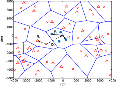
The target BS is considered to be placed at the origin, giving service to $k$ active users in $k$ orthogonal resource groups. Cells are assumed to be fully loaded, thus all available resource groups are used in the target and interfering cells and users are allocated a single resource group. These users, represented with blue dots, are ordered according to their distance to its serving BS, i.e. the origin. We focus on the $l^{th}$ user placed at distance $R_{l}$ from the origin with ${0\leq R_{1}\leq\cdots\leq R_{l}\leq\cdots\leq R_{k}}$. The BS positions of the interfering cells are indicated by red triangles, whereas the interfering users for the $l^{th}$ user data transmission are represented by red crosses.

Since fractional power control is considered, the transmitted power depends on the distance between the user and its serving BS. This distance is represented as $R_{x}$ for an interfering user placed at $x\in\Phi_{i,l}$, where $\Phi_{i,l}$ denotes the random set of interfering user locations for $l^{th}$ user data transmission. Similarly, the distance between the interfering user located at $x$ and the target BS (i.e. the origin) is represented as $D_{x}$.

Power loss due to propagation is modeled using a standard path loss model with $\alpha>2$, whereas a Rayleigh model is assumed for small-scale fading. Fractional power control with parameter $\epsilon$ is assumed, hence the received signal power at distance $D_{x}$ from a user placed at distance $R_{x}$ from its BS is given by $G_{x}R_{x}^{\alpha\epsilon}D_{x}^{-\alpha}$, where $G_{x}$ is the fading coefficient that follows an exponential distribution with mean $1/\mu$. Thus, the SINR for the $l^{th}$ user data transmission follows the next expression

$$\text{SINR}_{l}=\frac{G_{l}R_{l}^{\alpha(\epsilon-1)}}{I_{l}+\sigma^{2}}$$ (1)

where $\sigma^{2}$ is the AWGN noise power and $I_{l}$ accounts for the interference experienced by the $l^{th}$ user transmission, given by

$$I_{l}=\sum_{x\in\Phi_{i,l}}G_{x}R_{x}^{\alpha\epsilon}D_{x}^{-\alpha}$$ (2)

It is important to note that in the UL, the interference suffered by all $k$ users transmission has the same statistics since interfering users positions scheduled at each resource group are expected to have the same distribution. Hence, from now on we will omit the sub-index $l$ in $\Phi_{i}$ for notation simplicity.

II-B Proposed Analytical Model

The proposed model for multi-user uplink analysis is illustrated in Fig. 2. This model uses conditional thinning in order to deal with multiple active links within the cell of interest.

Figure 2: Multi-User UL set-up based on conditional thinning for $k=11$. Interfering users for the $l^{th}$ user transmission are represented with red crosses.

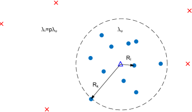
Let us consider the target BS to be placed at the origin and an uniform PPP $\Phi$ of intensity $\lambda$ over $\mathbb{R}^{2}$ that represents the set of active users. We use conditional thinning as follows:

First, the $k$ nearest points of $\Phi$ to the origin are selected. These points represent the locations of $k$ users scheduled in $k$ orthogonal resource groups. Then, thinning with probability $p$ is performed to all points except those $k$ inside the closed ball $B(o,r_{k})$, being $r_{k}$ the distance to the $k^{th}$ point.

The resulting set of points outside the ball $B(o,r_{k})$ is a non-uniform PPP $\Phi_{i}$ of intensity measure $\Lambda_{i}(A)=p\lambda|A\setminus B(o,r_{k})|$ [12]. Such random set of points represents the interfering user locations for the $l^{th}$ user data transmission. Since these interfering users are using one of $k$ available resources, we choose the thinning probability to be $p=1/k$. As the model considers that there is only one user scheduled per orthogonal resource group per cell, the intensity of BS is exactly the same as the intensity of interfering users. The random set of $k$ points around the origin $\Phi_{d}$ has an intensity measure $\Lambda_{d}(A)=\lambda|A\cap B(o,r_{k})|$. Hence, the complete set of user locations $\Phi_{u}$ is given by the set of user locations within the target cell (using all available resource groups) and the set of interfering users scheduled in one resource group, i.e. $\Phi_{u}=\Phi_{d}+\Phi_{i}$.

As in [7] distances $\{R_{x}\}$ from each interfering user to its serving BS are assumed to be i.i.d. RV following Rayleigh distributions with

$$f_{R_{x}}(r_{x})=2\pi p\lambda r_{x}\mathrm{e}^{-p\lambda\pi r_{x}^{2}},\,r_{x}\geq 0$$ (3)

Hence, notice that the proposed model is equivalent to the model presented in [7] for $p=1$, and $k=l=1$.

II-C Simulation Model

In order to asses the validity of the proposed analysis model, we also introduce a more realistic model for simulation. A uniform PPP of intensity $\lambda_{b}$ representing the BS locations is first considered. Since in the analysis model the intensity of BS is the same as that of interfering users, we use $\lambda_{b}=\lambda/k$ aiming to compare the results of both models.

The association between user and BS is based on distance, hence the Voronoi tessellation is performed where one randomly chosen point is the target BS. Then, $k$ points representing the $k$ active users are placed randomly inside the target cell, whereas only one user is placed in each interfering cell. Notice that both sets of points, active users inside the target cell and interfering users, are not a PPP. To explain that, recall that the number of points falling in a Voronoi cell tends to be higher as the cell is bigger; in our case, one interfering user falls in any cell independently of its size.

III Mathematical Results

After presenting the analytical framework for the analysis of multi-user UL cellular networks, we now present the main mathematical contributions of this paper. First, we derive the joint distribution of the distances between the $l^{th}$ and $k^{th}$ users and the serving BS. Then, we use this result to calculate the coverage probability of the $l^{th}$ user in the investigated scenario.

III-A Joint Distribution of Distances

In the analytical model, the $k$ users of interest are ordered according to their distances to the serving BS (i.e., the origin), and the interfering users are located at a distance greater than $R_{k}$. This interdependence affects the distribution of the SINR for the $l^{th}$ user transmission, due to the inherent correlation between $R_{l}$ and $R_{k}$. In the next lemma, we calculate their joint pdf.

Lemma 1

The joint pdf of $R_{l}$ and $R_{k}$ with $0<l<k$ is

$$f_{R_{l},R_{k}}(r_{l},r_{k})=\frac{4\mathrm{e}^{-\pi r_{k}^{2}\lambda}(\lambda\pi)^{k}r_{k}r_{l}^{2l-1}(r_{k}^{2}-r_{l}^{2})^{k-l-1}}{(k-l-1)!(l-1)!}$$ (4)

where $0\leq r_{l}\leq r_{k}$.

Proof:

The calculation of the joint pdf follows a similar procedure as in [10]. Hence, we define disjoint sets in order to use the independence property of the PPP. Let us consider the next disjoint sets

$$\Psi_{1}=\{x\in\mathbb{R}^{2}:\lVert x\rVert\leq r_{l}\}$$

$$\Psi_{2}=\{x\in\mathbb{R}^{2}:r_{l}<\lVert x\rVert\leq r_{l}+\mathrm{d}r_{l}\}$$

$$\Psi_{3}=\{x\in\mathbb{R}^{2}:r_{l}+\mathrm{d}r_{l}<\lVert x\rVert\leq r_{k}\}$$

$$\Psi_{4}=\{x\in\mathbb{R}^{2}:r_{k}<\lVert x\rVert\leq r_{k}+\mathrm{d}r_{k}\}$$ (5)

The joint pdf of $R_{l}$ and $R_{k}$ with $0<l<k$ is by definition

$$f_{R_{l},R_{k}}(r_{l},r_{k})=\lim_{\overset{\mathrm{d}r_{l}\to 0}{\underset{\mathrm{d}r_{k}\to 0}{}}}\frac{\mathbb{P}\{R_{l}\in\Psi_{2},R_{k}\in\Psi_{4}\}}{\mathrm{d}r_{l}\mathrm{d}r_{k}}$$ (6)

Notice that the numerator can be expressed as follows:

$$\mathbb{P} \{R_{l}\in\Psi_{2},R_{k}\in\Psi_{4}\}=$$

$$\mathbb{P}\{\Phi(\Psi_{1})=l-1\}\cdot\mathbb{P}\{\Phi(\Psi_{2})=1\}\cdot$$

$$\mathbb{P}\{\Phi(\Psi_{3})=k-l-1\}\cdot\mathbb{P}\{\Phi(\Psi_{4})=1\}$$ (7)

being $\Phi(\Psi)$ a random counting measure of a Borel set $\Psi$. Since $\Phi$ is a uniform PPP, $\Phi(\Psi)$ follows Poisson distribution with mean $\lambda\lvert\Psi\rvert$ [12]. Substituting the probability of each event in (III-A) and calculating the limits in (6) yields the desired pdf. ∎

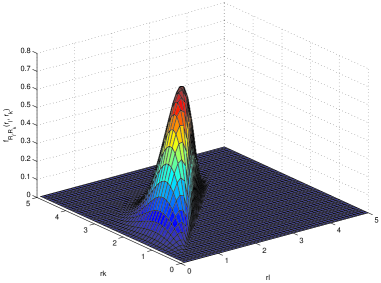
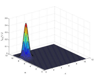
Figs. 3 and 4 illustrate the joint pdf of the distances for the second and the $k^{th}$ user, when $k=4$ and $k=50$, respectively. The correlation is more noticeable when $l$ and $k$ have similar values.

Figure 3: Joint pdf for $l=2$ and $k=4$ with $\lambda=0.24$

Figure 4: Joint pdf for $l=2$ and $k=50$ with $\lambda=0.24$

III-B Multi-User Coverage Probability

The coverage probability represents the probability for a user to have a SINR higher than certain threshold $t$. The main result is stated in Theorem 1, which corresponds to the coverage probability of the the $l^{th}$ user.

Theorem 1 (Multi-user coverage probability)

The coverage probability of the $l^{th}$ user considering a system with $k$ orthogonal resource groups that are distributed among $k$ active users with $l<k$ is given by:

$$p_{c}(l,k,t,\lambda, p,\alpha,\epsilon,\mu,\sigma^{2})$$

$$=\mathbb{E}_{R_{l},R_{k}}\left[\xi(r_{l},r_{k})\right]$$

$$=\int_{0}^{\infty}\int_{r_{l}}^{\infty}\xi(r_{l},r_{k})f_{R_{l},R_{k}}(r_{l},r_{k})\mathrm{d}r_{k}\mathrm{d}r_{l}$$ (8)

where $f_{R_{l},R_{k}}(r_{l},r_{k})$ is the joint pdf of distances and

$$\xi(r_{l},r_{k})=\mathrm{e}^{-\mu t\sigma^{2}r_{l}^{\alpha(1-\epsilon)}}\mathcal{L}_{I_{l}|r_{l},r_{k}}(\mu tr_{l}^{\alpha(1-\epsilon)})$$ (9)

being $\mathcal{L}_{I_{l}|r_{l},r_{k}}(s)$ the Laplace transform of the interference conditioned on $r_{l}$ and $r_{k}$. This term evaluated at $s=\mu tr_{l}^{\alpha(1-\epsilon)}$ has the following expression

$$\mathcal{L}_{I_{l}|r_{l},r_{k}}(\mu tr_{l}^{\alpha(1-\epsilon)})=$$

$$\mathrm{exp}\left(-2\pi p\lambda\int_{r_{k}}^{\infty}\left(1-\int_{0}^{\infty}\frac{\pi p\lambda\mathrm{e}^{-p\lambda\pi q}}{1+tr_{l}^{\alpha(1-\epsilon)}q^{\alpha\epsilon/2}v^{-\alpha}}\mathrm{d}q\right)v\mathrm{d}v\right)$$ (10)

Proof:

The coverage probability for the $l^{th}$ user can be expressed as

$$p_{c}( l,k,t,\lambda,p,\alpha,\epsilon,\mu,\sigma^{2})=\mathbb{P}\left[\mathrm{SINR}_{l}>t\right]$$

$$\overset{(a)}{=}\int_{0}^{\infty}\mathbb{P}\left[\mathrm{SINR}_{l}>t\rvert r_{l}\right]f_{R_{l}}(r_{l})\mathrm{d}r_{l}$$

$$=\int_{0}^{\infty}\mathbb{P}\left[G_{l}>t(I_{l}+\sigma^{2})r_{l}^{\alpha(\epsilon-1)}\rvert r_{l}\right]f_{R_{l}}(r_{l})\mathrm{d}r_{l}$$

$$\overset{(b)}{=}\int_{0}^{\infty}\mathbb{E}_{I_{l}}\left[\mathbb{P}\left[G_{l}>t(i_{l}+\sigma^{2})r_{l}^{\alpha(\epsilon-1)}\rvert r_{l},i_{l}\right]\right]f_{R_{l}}(r_{l})\mathrm{d}r_{l}$$

$$\overset{(c)}{=}\int_{0}^{\infty}\mathrm{e}^{-\mu t\sigma^{2}r_{l}^{\alpha(\epsilon-1)}}\mathbb{E}_{I_{l}|r_{l}}\left[\mathrm{e}^{-\mu tI_{l}r_{l}^{\alpha(\epsilon-1)}}\rvert r_{l}\right]f_{R_{l}}(r_{l})\mathrm{d}r_{l}$$ (11)

where $(a)$ and $(b)$ follow from the total probability theorem [13], while $(c)$ follows from the fact that $G_{l}$ has an exponential distribution with mean $1/\mu$.

The term $\mathcal{L}_{I_{l}|r_{l}}(s)=\mathbb{E}_{I_{l}|r_{l}}\left[\mathrm{e}^{I_{l}}\rvert r_{l}\right]$ represents the Laplace transform of the interference conditioned on $r_{l}$. The RV $R_{l}$ and $R_{k}$ are correlated as $R_{l}\leq R_{k}$. Since $I_{l}$ depends on $R_{k}$ due to the fact that the interfering users are placed farther than $R_{k}$, the RV $I_{l}$ also depends on $R_{l}$. Hence we have to deal with such dependence as follows

$$\mathcal{L}_{I_{l}|r_{l}}(s) =\mathbb{E}_{I_{l}|r_{l},r_{k}}\left[\mathbb{E}_{R_{k}}\left[\mathrm{e}^{-sI_{l}}\rvert r_{l},r_{k}\right]\right]$$

$$=\mathbb{E}_{I_{l}|r_{l},r_{k}}\left[\int_{r_{l}}^{\infty}\mathrm{e}^{-sI_{l}}f_{R_{k}\lvert r_{l}}(r_{k})\mathrm{d}r_{k}\rvert r_{l},r_{k}\right]$$

$$=\int_{r_{l}}^{\infty}\mathbb{E}_{I_{l}|r_{l},r_{k}}\left[\mathrm{e}^{-sI_{l}}\rvert r_{l},r_{k}\right]f_{R_{k}\lvert r_{l}}(r_{k})\mathrm{d}r_{k}$$ (12)

where the total probability theorem and linearity of expectation operator have been used.

The term $\mathcal{L}_{I_{l}|r_{l},r_{k}}(s)=\mathbb{E}_{I_{l}|r_{l},r_{k}}\left[\mathrm{e}^{-sI_{l}}\rvert r_{l},r_{k}\right]$ stands for the Laplace transform of the interference conditioned on $r_{l}$ and $r_{k}$ and can be expressed as

$$\mathcal{L}_{I_{l}|r_{l},r_{k}}(s)=\mathbb{E}_{\Phi_{i},\{G_{x}\}}\left[\mathrm{e}^{-s\sum_{x\in\Phi_{i}}G_{x}R_{x}^{\alpha\epsilon}D_{x}^{-\alpha}}\right]$$

$$\overset{(a)}{=}\mathbb{E}_{R_{x},D_{x}}\left[\prod_{x\in\Phi_{i}}\mathbb{E}_{G_{x}}\left[\mathrm{e}^{-sG_{x}R_{x}^{\alpha\epsilon}D_{x}^{-\alpha}}\right]\right]$$

$$\overset{(b)}{=}\mathbb{E}_{D_{x}}\left[\prod_{x\in\Phi_{i}}\mathbb{E}_{R_{x}}\left[\frac{\mu}{\mu+sR_{x}^{\alpha\epsilon}D_{x}^{-\alpha}}\right]\right]$$

$$\overset{(c)}{=}\exp\left(-2\pi\lambda p\int_{r_{k}}^{\infty}\left(1-\int_{0}^{\infty}\frac{\pi p\lambda\mathrm{e}^{-p\lambda\pi q}\mathrm{d}q}{1+tr_{l}^{\alpha(1-\epsilon)}q^{\frac{\alpha\epsilon}{2}}v^{-\alpha}}\right)v\mathrm{d}v\right)$$ (13)

where the dependence with $R_{l}$ and $R_{k}$ resides in the non-uniform PPP $\Phi_{i}$ since its intensity is $\Lambda_{i}(A)=p\lambda|A\setminus B(o,r_{k})|$. Step $(a)$ comes from the fact that the fading is independent of the PPP, $(b)$ comes from the independence assumption between $R_{x}$ and $D_{x}$ and $(c)$ from the Probability Generating Functional (PGFL) [12] and the assumption of $R_{x}$ following a Rayleigh distribution as in [7].

Substituting (III-B) and (III-B) with $s=\mu tr_{l}^{\alpha(1-\epsilon)}$ in (III-B) and taking into account that the conditional pdf $f_{R_{k}\lvert r_{l}}(r_{k})$ can be obtained from the joint pdf and the marginal pdf of $R_{l}$ as $f_{R_{k}\lvert r_{l}}(r_{k})=f_{R_{l},R_{k}}(r_{l},r_{k})/f_{R_{l}}(r_{l})$, the proof is completed. ∎

Theorem 1 provides the coverage probability of the $l^{th}$ user with $l<k$. The following lemma gives the coverage probability for the cell-edge user.

Lemma 2

The coverage probability of the $k^{th}$ user follows the next expression

$$p_{c}(k,t,\lambda,p,\alpha,\epsilon,\mu,\sigma^{2})=\int_{0}^{\infty}\xi(r_{k})f_{R_{k}}(r_{k})\mathrm{d}r_{k}$$ (14)

where $f_{R_{k}}(r_{k})$ is the marginal pdf distribution of the $k^{th}$ nearest point [14] given by

$$f_{R_{k}}(r_{k})=2\frac{(\lambda\pi)^{k}}{(k-1)!}r_{k}^{2k-1}\mathrm{e}^{-\lambda\pi r_{k}^{2}}$$ (15)

and

$$\xi(r_{k})=\mathrm{e}^{-\mu t\sigma^{2}r_{k}^{\alpha(1-\epsilon)}}\mathcal{L}_{I_{k}|r_{k}}(\mu tr_{k}^{\alpha(1-\epsilon)})$$ (16)

where $\mathcal{L}_{I_{k}|r_{k}}(\mu tr_{k}^{\alpha(1-\epsilon)})$ the Laplace transform of the interference affecting the $k^{th}$ user transmission conditioned on $r_{k}$, given by

$$\mathcal{L}_{I_{k}|r_{k}}(\mu tr_{k}^{\alpha(1-\epsilon)})=$$

$$\mathrm{exp}\left(-2\pi p\lambda\int_{r_{k}}^{\infty}\left(1-\int_{0}^{\infty}\frac{\pi p\lambda\mathrm{e}^{-p\lambda\pi q}}{1+tr_{k}^{\alpha(1-\epsilon)}q^{\alpha\epsilon/2}v^{-\alpha}}\mathrm{d}q\right)v\mathrm{d}v\right)$$ (17)

Proof:

The proof is analogous to Theorem 1 except from the fact that the SINR of the $k^{th}$ user transmission only depends on the distance to the origin of one particular user; note that when $l<k$ the SINR depends both on $R_{l}$ and $R_{k}$. Hence, the Laplace transform of the interference only depends on $R_{k}$ and only the marginal pdf of $R_{k}$ is necessary. ∎

IV Numerical Results

IV-A Coverage probability

We now evaluate the expressions for the coverage probability previously derived, and compare these results with our simulation model. Different values of the power control factor $\epsilon$ are used so as to provide a clear understanding of the relation between power control and fairness among users.

Fig. 5 shows the coverage probability considering different numbers of orthogonal resources per cell, i.e. $k=\{10,25,50\}$, assuming a full power control policy ($\epsilon=1$). We see how the coverage probability is the same for all $k$ scheduled users, i.e. it does not depend on $l$ for both analytical and simulation models. This is coherent with the fact that full compensation of path loss makes all user transmissions to have the same average received power. Since the interference experienced by all user transmissions is the same, the coverage is also the same. Hence, in this case the fairness between users is maximal. We also observe how the analytical model provides slightly more pessimistic results than the simulation model.

Figure 5: Coverage probability for $k=\{10,25,50\}$ with full power control ($\epsilon=1$), without noise, $\alpha=2.5$, $\lambda_{b}=0.24$

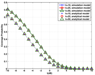
Fig. 6 illustrates the coverage probability for cell-interior ($l=1$) and cell-edge ($l=k$) users with $k=25$ and a power control factor $\epsilon=0.75$. We observe how both analytical and simulation models still behave quite close to each other. In both models, since the compensation of path loss is not total, transmissions from users closer to the BS are associated to higher SINR values than those in the cell-edge, so there exists a difference in coverage between users.

Figure 6: Coverage probability for cell-interior $l=1$ and cell-edge $l=k$ with $k=25$, $\epsilon=0.75$, without noise, $\alpha=2.5$, $\lambda_{b}=0.24$

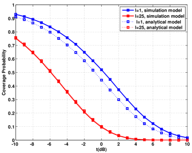
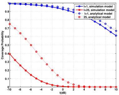
Fig. 7 shows the coverage probability in the absence of power control, which corresponds to the worse case in terms of fairness. Hence, we observe that the difference in coverage between cell-interior $l=1$ and cell-edge $l=k$ users is maximal. We also see how for the cell-edge user the analytical model yields a coverage significantly greater than the simulation model. The reason behind that is related to the different distribution of points used to model active user locations in both models. As mentioned in section II, in the analytical model user locations form a PPP, whereas in the simulation model this does not hold. This issue has a significant impact on the pdf of the distances $R_{l}$ specially for cell-edge users, and is addressed in detail in the next subsection.

Figure 7: Coverage probability for cell-interior $l=1$ and cell-edge $l=k$ with $k=25$, without power control $\epsilon=0$, without noise, $\alpha=2.5$, $\lambda_{b}=0.24$

IV-B Marginal distributions of distances

One of the assumptions of the proposed model follows from [7] and states that $R_{x}$ with $x\in\Phi_{i}$ are i.i.d. Rayleigh distributed RVs. Fig. 8 shows the theoretical (Rayleigh) distribution used in the analytical model and the empirical distribution obtained from the simulation model. We observed that both pdfs are quite similar, so it is expected that the statistics of the transmitted power of the interfering users are also close to each other.

Figure 8: Empirical and theoretical pdf of $R_{x}$.

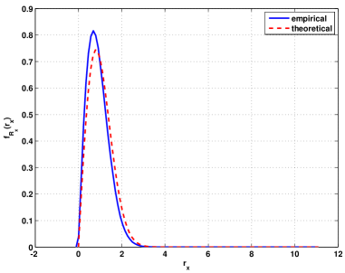
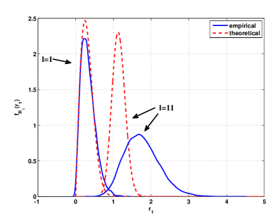
Fig. 9 shows the marginal pdfs of $R_{l}$ for the closest and the farthest user to the target BS. For the cell-interior user ($l=1$) we see that both the empirical and theoretical pdfs are rather similar; hence, we may expect that coverage results from both models are also similar (as illustrated in the previous figures). However, for cell-edge users both pdfs have different shapes. Specifically, we notice that the distances of cell-edge users in the analytical model tend to be lower than the distances in the simulation model. This explains the difference in coverage probability, specially in the absence of power control as exhibited in Fig. 7. Since the distance for the cell-edge user tends to be lower in the analytical model when power control is not used, the desired signal tends to be higher and so the coverage probability grows. This is mitigated by using power control, since this technique aims to obtain equal received power from all users independently of their positions.

Figure 9: Empirical and theoretical pdfs of $R_{l}$, ($l=1,k=11$) and ($l=k=11$)

V Conclusions

We proposed a tractable analysis model for multi-user uplink cellular networks based on conditional thinning. Assuming that there are $k$ active users scheduled on $k$ orthogonal resources, the joint distribution of the distances from the target BS to the $l^{th}$ user and to the farthest $k^{th}$ user have been obtained. Thinning outside the target cell with probability $1/k$ is used to obtain the actual set of interfering users. A more realistic model with BS distributed as PPP and one interfering user within its Voronoi cell has been simulated as well. Results show that fractional power control permits to increase fairness among users, at the expense of reducing the coverage probability of cell-interior users as $\epsilon$ grows. The coverage results provided by the analysis model are close to the simulation models when power control is used; the difference of behavior in the absence of power control is also discussed by studying the marginal distributions of the distances of the users to the serving BS.

References

- [1] N. Himayat, S. Talwar, A. Rao, and R. Soni, “Interference management for 4G cellular standards [WIMAX/LTE UPDATE],” IEEE Communications Magazine, vol. 48, no. 8, pp. 86–92, Aug. 2010.
- [2] A. D. Wyner, “Shannon-theoretic approach to a Gaussian cellular multiple-access channel,” IEEE Transactions on Information Theory, vol. 40, no. 6, pp. 1713–1727, 1994.
- [3] A. Tukmanov, Z. Ding, S. Boussakta, and A. Jamalipour, “On the impact of network geometric models on multicell cooperative communication systems,” IEEE Wireless Commun., vol. 20, no. 1, pp. 75–81, Feb. 2013.
- [4] J. Xu, J. Zhang, and J. G. Andrews, “On the Accuracy of the Wyner Model in Cellular Networks,” IEEE Transactions on Wireless Communications, vol. 10, no. 9, pp. 3098–3109, Sep. 2011.
- [5] M. Haenggi, J. G. Andrews, F. Baccelli, O. Dousse, and M. Franceschetti, “Stochastic geometry and random graphs for the analysis and design of wireless networks,” IEEE Journal on Selected Areas in Communications, vol. 27, no. 7, pp. 1029–1046, Sep. 2009.
- [6] J. G. Andrews, F. Baccelli, and R. K. Ganti, “A Tractable Approach to Coverage and Rate in Cellular Networks,” IEEE Transactions on Communications, vol. 59, no. 11, pp. 3122–3134, Nov. 2011.
- [7] T. D. Novlan, H. S. Dhillon, and J. G. Andrews, “Analytical Modeling of Uplink Cellular Networks,” IEEE Transactions on Wireless Communications, vol. 12, no. 6, pp. 2669–2679, June 2013.
- [8] T. D. Novlan and J. G. Andrews, “Analytical Evaluation of Uplink Fractional Frequency Reuse,” IEEE Transactions on Communications, vol. 61, no. 5, pp. 2098–2108, May 2013.
- [9] H. ElSawy and E. Hossain, “On Stochastic Geometry Modeling of Cellular Uplink Transmission with Truncated Channel Inversion Power Control,” arXiv preprint arXiv:1401.6145, 2014.
- [10] H. S. Dhillon, R. K. Ganti, and J. G. Andrews, “Modeling Non-Uniform UE Distributions in Downlink Cellular Networks,” IEEE Wireless Communications Letters, vol. 2, no. 3, pp. 339–342, June 2013.
- [11] ——, “Load Aware Modeling and Analysis of Heterogeneous Cellular Networks,” IEEE Transactions on Wireless Communications, vol. 12, no. 4, pp. 1666–1677, Apr. 2013.
- [12] S. N. Chiu, D. Stoyan, W. S. Kendall, and J. Mecke, Stochastic Geometry and Its Applications. Wiley Series in Probability and Statistics, 2013.
- [13] A. Papoulis and S. U. Pillai, Probability, Random Variables, and Stochastic Processes, ser. McGraw-Hill series in electrical engineering: Communications and signal processing. Tata McGraw-Hill, 2002.
- [14] M. Haenggi, “On distances in uniformly random networks,” IEEE Transactions on Information Theory, vol. 51, no. 10, pp. 3584–3586, Oct 2005.