Self-force on a charge outside a five-dimensional black hole

Abstract

We compute the electromagnetic self-force acting on a charged particle held in place at a fixed position $r$ outside a five-dimensional black hole described by the Schwarzschild-Tangherlini metric. Using a spherical-harmonic decomposition of the electrostatic potential and a regularization prescription based on the Hadamard Green’s function, we express the self-force as a convergent mode sum. The self-force is first evaluated numerically, and next presented as an analytical expansion in powers of $R/r$, with $R$ denoting the event-horizon radius. The power series is then summed to yield a closed-form expression. Unlike its four-dimensional version, the self-force features a dependence on a regularization parameter $s$ that can be interpreted as the particle’s radius. The self-force is repulsive at large distances, and its behavior is related to a model according to which the force results from a gravitational interaction between the black hole and the distribution of electrostatic field energy attached to the particle. The model, however, is shown to become inadequate as $r$ becomes comparable to $R$, where the self-force changes sign and becomes attractive. We also calculate the self-force acting on a particle with a scalar charge, which we find to be everywhere attractive. This is to be contrasted with its four-dimensional counterpart, which vanishes at any $r$.

I Introduction and summary

A particle held in place at a fixed position $r$ outside a nonrotating black hole of mass $M$ requires an external agent to supply an external force $F_{\rm ext}$ that compensates for the black hole’s gravity. When the particle carries an electric charge $q$, the external force is smaller than when the particle is neutral. The difference is accounted for by the particle’s electromagnetic self-force, which originates in a subtle interaction between the particle, the electric field it generates, and the spacetime curvature around the black hole. The electromagnetic self-force acting on a charged particle at rest outside a Schwarzschild black hole was computed by Smith and Will smith-will:80 . The only nonvanishing component of the force vector $F^{\alpha}$ is the radial component $F^{r}$, and the force invariant $F:=\pm\sqrt{g_{\alpha\beta}F^{\alpha}F^{\beta}}$, with the sign adjusted so that the sign of $F$ agrees with the sign of $F^{r}$, is given by

$$F=\frac{q^{2}R}{2r^{3}},$$ (1)

where $R=2M$ is the event-horizon radius (we use geometrized units, in which $G=c=1$). The positive sign on the right-hand side indicates that the self-force is repulsive, which leads to a smaller $F_{\rm ext}$ when the particle carries a charge.

The repulsive nature of the electromagnetic self-force is a surprising feature that is difficult to explain. An attempt to provide some intuition relies on the fact that the event horizon is necessarily an equipotential surface, which suggests that the black hole should behave as a perfect conductor. This observation leads to the expectation that the self-force could be derived (up to numerical factors) on the basis of an elementary model involving a spherical conductor of radius $R$ in flat spacetime. The model features a charge $q$ at position $r$, a first image charge $q^{\prime}=-q(R/r)$ at position $R^{2}/r$ inside the conductor, and a second image charge $-q^{\prime}=q(R/r)$ at the center. The first image charge produces a grounded conductor with a net charge $q^{\prime}$ distributed on its surface, and the second image charge eliminates this net charge, without violating the equipotential condition at the surface. (The black hole does not support a net charge.) The model predicts a self-force resulting from an interaction between the charge $q$ and the image dipole inside the conductor, and a simple calculation neglecting corrections of order $(R/r)^{2}$ reveals that the self-force scales as $F\sim-q^{2}R^{3}/r^{5}$, with a negative sign indicating an attractive force. The model is a complete failure: it fails to produce to the correct scaling with $R$ and $r$, and it even fails to produce the correct sign.

Another attempt to provide intuition, proposed in Sec. IV of Ref. burko-etal:00 , produces a more intelligible picture. This model focuses its attention on the force acting on the black hole instead of the force acting on the charged particle. This force is necessarily gravitational in nature, and according to Newton’s third law, it must be equal in magnitude to the force acting on the particle. (The model features a mixture of Newtonian and relativistic ideas.) The force on the black hole is produced in part by the particle’s mass, but there is also a contribution from the distribution of electrostatic field energy that surrounds the charge. In this view, the charged particle behaves as an infinitely extended body, and the black hole is comparatively much smaller. The force on the black hole is then $F_{\rm hole}=-Mm(r)/r^{2}$, with the negative sign indicating that the force is attractive, and $m(r)$ denoting the mass within radius $r$ associated with the particle and the distribution of field energy. The particle’s mass $m$ is identified with $m(\infty)$, and $m(r)=m-\int_{r}^{\infty}4\pi\rho r^{2}\,dr$, where $\rho=E^{2}/(8\pi)$ is the density of field energy. With $E=q/r^{2}$ we have that $m(r)=m-q^{2}/(2r)$, and the force becomes $F_{\rm hole}=-Mm/r^{2}+q^{2}R/(4r^{3})$. The first term is the attractive gravitational force exerted by the particle, and the second term is a repulsive contribution from the field energy. Writing $F_{\rm charge}=F_{\rm hole}$ gives us an alternative interpretation: the first term is the gravitational force exerted by the black hole, and the second term is the self-force. This model is a success: it produces the correct scaling with $R$ and $r$, and it produces the correct sign. It reproduces the Smith-Will force of Eq. (1) up to a factor of 2.

The failure of the electrostatic model at providing a reliable expression for the self-force has been a source of fascination in the literature, and it has motivated a line of inquiry that probes into the mysteries of the self-force in various circumstances. Thus, authors have replaced the black hole with various material bodies unruh:76 ; burko-etal:00 ; shankar-whiting:07 ; drivas-gralla:11 ; isoyama-poisson:12 ; they observed that the Smith-Will behavior of Eq. (1) is universal at large distances, but modified when $r$ becomes comparable to the body’s radius $R$. Other authors have replaced the asymptotically-flat boundary conditions of the Schwarzschild spacetime by asymptotic cosmological conditions (specifically, de Sitter or anti de Sitter conditions kuchar-poisson-vega:13 ); they observed that the Smith-Will behavior continues to hold approximately when the black-hole and cosmological scales are well separated, but is substantially modified when the scales are comparable.

In this paper we continue this line of inquiry, and ask whether the interpretation of the self-force as a gravitational interaction between the black hole and the electrostatic field energy attached to the particle continues to apply in higher dimensions. Extending the model to an $(n+2)$-dimensional spacetime, with $n$ denoting the number of angular directions, we have that the force on the black hole is now given by $F_{\rm hole}=-Mm(r)/r^{n}$. The mass within radius $r$ becomes $m(r)=m-\int_{r}^{\infty}\Omega_{n}\rho r^{n}\,dr$, where $\rho=E^{2}/(2\Omega_{n})$ is the density of field energy, and $\Omega_{n}$ is the area of a unit $n$-sphere. With $E=q/r^{n}$ we have that $m(r)=m-q^{2}/[2(n-1)r^{n-1}]$, and we obtain $F_{\rm hole}=-Mm/r^{n}+q^{2}M/[2(n-1)r^{2n-1}]$. The second term is identified with the electromagnetic self-force, and relating the black-hole mass to its event-horizon radius $R$ via $M=\frac{1}{2}(n-1)R^{n-1}$, we arrive at an expected scaling of $q^{2}R^{n-1}/(4r^{2n-1})$ for the self-force. We wish to know whether this expectation is borne out by an actual computation. Self-forces in higher-dimensional spacetimes were also considered by Frolov and Zelnikov frolov-zelnikov:12a ; frolov-zelnikov:12b ; frolov-zelnikov:12c ; frolov-zelnikov:12d , who provided concrete results for the specific case of Majumdar-Papapetrou spacetimes.

For reasons that will be explained below, our calculation of the self-force is restricted to the five-dimensional case. We obtain

$$F=\frac{q^{2}R^{2}}{2r^{5}}\,\frac{\Xi}{f^{3/2}},$$ (2)

where $R$ is the event-horizon radius, $f:=1-(R/r)^{2}$, and

$$\Xi=-\frac{1}{4x}+\frac{5}{8}+\frac{139}{96}\,x-\frac{281}{192}\,x^{2}+\biggl{(}\frac{1}{4x}+\frac{1}{2}-\frac{15}{16}\,x\biggr{)}\sqrt{f}+\frac{3}{16}\,x(6-5x)\ln\frac{\tilde{s}x(1+\sqrt{f})}{8\sqrt{f}}$$ (3)

with $x:=(R/r)^{2}$. The self-force depends on an unknown parameter, the dimensionless quantity $\tilde{s}:=s/R$, which originates in the regularization prescription to be described below. An interpretation for the length scale $s$ is that it represents the radius of the particle, which must of course be much smaller than the black hole, so that $\tilde{s}\ll 1$. The self-force, therefore, is not independent of the particle’s size, and presumably this is an indication that in five dimensions, the self-force cannot be expected to be independent of the details of internal structure. A graph of $\Xi/f^{3/2}$ for selected values of $\tilde{s}$ is displayed in Fig. 1.

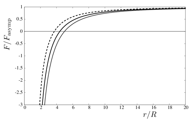
Figure 1: Electromagnetic self-force acting on a particle of charge $q$ at a fixed position $r$ in the five-dimensional Schwarzschild-Tangherlini spacetime. The self-force $F$ is divided by its asymptotic expression $F_{\rm asymp}=q^{2}R^{2}/(2r^{5})$, and it is plotted as a function of $r/R$ for $\tilde{s}=10^{-4}$ (long-dashed curve), $\tilde{s}=10^{-6}$ (solid curve), and $\tilde{s}=10^{-8}$ (short-dashed curve). The self-force is positive (repulsive) when $r/R$ is sufficiently large, but it changes sign and becomes attractive when $r/R$ becomes comparable to 4. For $\tilde{s}=10^{-4}$ the transition occurs at $r/R\simeq 3.7154$, for $\tilde{s}=10^{-6}$ it occurs at $r/R\simeq 4.4010$, and for $\tilde{s}=10^{-8}$ it occurs at $r/R\simeq 4.9830$.

When $r$ is large compared with $R$, the function $\Xi/f^{3/2}$ behaves as $1+O(x)$, and the self-force becomes

$$F\sim\frac{q^{2}R^{2}}{2r^{5}},\qquad(r\gg R).$$ (4)

This repulsive behavior matches the expectation from the gravitational model, up to a factor of two that was also seen in the four-dimensional case. When $r$ decreases toward $R$, however, the self-force force changes sign and becomes attractive. As $r$ approaches $R$ the diverging factor $f^{-3/2}$ begins to dominate, but the divergence is limited by the fact that the particle cannot be closer to the horizon than a distance of order $s$. Taking $r/R>1+\tilde{s}$, we find that the self-force is bounded by

$$F>-\frac{3}{128\sqrt{2}}\frac{q^{2}}{R^{3}}\frac{1}{\tilde{s}^{3/2}}\ln\frac{128}{\tilde{s}}.$$ (5)

In spite of this bound, the behavior of the self-force very close to the horizon should be viewed with suspicion, because a large $|F|$ implies a large electric field that can no longer be treated as a test field in a fixed background spacetime. The detailed description of the self-force reveals that the interpretation in terms of a gravitational interaction does not hold up to five-dimensional scrutiny. While the large-$r$ behavior of the self-force is repulsive and compatible with the model, the agreement does not persist when $r$ becomes comparable to $R$.

Unlike Smith and Will, our computation of the five-dimensional self-force does not proceed on the basis of an exact solution to Maxwell’s equations for a point charge in the Schwarzschild-Tangherlini spacetime. Indeed, such a five-dimensional analogue of the Copson solution copson:28 ; linet:76 is not known. Our method of calculation is therefore more convoluted. We begin in Sec. II with the formulation of Maxwell’s equations in higher-dimensional spacetimes, their specialization to the specific case of a point charge in the Schwarzschild-Tangherlini spacetime, and a presentation of the solution in terms of a decomposition in higher-dimensional spherical harmonics. This leads to a self-force expressed as an infinite and diverging sum over spherical-harmonic modes.

The mode-sum evaluation of the self-force requires regularization, and we carry out the necessary steps in Sec. III. We adopt a regularization prescription based on Hadamard’s Green’s function hadamard:23 , a local expansion of the electrostatic potential that identifies the singular part that must be subtracted before the mode sum is evaluated. While Hadamard regularization can be formulated in any spacetime dimension, its practical implementation becomes increasingly difficult as the number of dimensions increases, for the simple reason that the electric field of a point charge becomes increasingly singular at the position of the particle. With the techniques at our disposal we were able to handle the five-dimensional case with relative ease, and this motivated our restriction to five dimensions. An extension to higher dimensions is possible, but would require a substantial amount of additional work.

Unlike the situation in four dimensions, the five-dimensional Hadamard Green’s function features a logarithmic dependence on the separation between field and source points. This is the source of the $\ln(s/R)$ term in the self-force, with the length parameter $s$ interpreted as the particle’s radius. Unlike its four-dimensional version, the five-dimensional self-force depends on the details of the particle’s internal structure. This dependence is likely to be even more dramatic in higher dimensions, because the field of a point charge becomes increasingly singular and requires additional regularization. It would be interesting to pursue these matters by performing a self-force calculation in six dimensions.

The calculation of the self-force proceeds in Sec. IV with a numerical evaluation of the regularized mode sum, and an analytical evaluation presented as an expansion in powers of $R/r$. We carry out this expansion to a very high order, and manage to sum the series to the closed-form expression displayed in Eq. (2).

In Sec. V we exploit the same methods to calculate the self-force acting on a scalar charge $q$ at a fixed position $r$ in the five-dimensional Schwarzschild-Tangherlini spacetime. Our final result is displayed in Eq. (141) below. When $r$ is much larger than $R$ we find that the scalar self-force behaves as

$$F_{\rm scalar}\sim-\frac{3}{8}\frac{q^{2}R^{4}}{r^{7}}\ln\frac{2r}{\sqrt{\tilde{s}}R}.$$ (6)

The self-force is attractive everywhere, and its scaling with $R^{4}\ln r/r^{7}$ can be contrasted with the $R^{2}/r^{5}$ scaling of the electromagnetic self-force. This result can also be contrasted with Wiseman’s four-dimensional expression wiseman:00 : $F_{\rm scalar}=0$. Like its electromagnetic counterpart, the scalar self-force is bounded by Eq. (5) when the particle is close to the horizon.

What would happen to the five-dimensional self-force if the topology of the event horizon were changed from the $S^{3}$ topology examined here to the $S^{2}\times\mathbb{R}$ topology of a black string? The regularization techniques developed in this paper could be adapted to this new situation, and a fresh calculation of the self-force could be attempted. Would the self-force continue to diverge as the event horizon is approached? We hope to return to this question in future work. In the remainder of the paper we present the detailed calculations that lead to the results summarized in this introductory section.

II Electrostatics in a higher-dimensional black-hole spacetime

In this section we formulate Maxwell’s equations in a curved spacetime of arbitrary dimensionality, and specialize them to the description of a static electric charge in the spacetime of a nonrotating black hole. This spacetime is static and spherically symmetric, and we denote the number of angular directions by $n$; the total number of spatial dimensions is then $n+1$, and $n+2$ is the number of spacetime dimensions.

II.1 Maxwell’s equations and Lorentz force

Maxwell’s equations in a curved, $(n+2)$-dimensional spacetime are expressed in covariant form as

$$\nabla_{\beta}F^{\alpha\beta}=\Omega_{n}j^{\alpha},\qquad\nabla_{[\alpha}F_{\beta\gamma]}=0,$$ (7)

where $F^{\alpha\beta}$ is the electromagnetic field tensor, $j^{\alpha}$ is the current density, $\nabla_{\alpha}$ is the covariant derivative operator, and $\Omega_{n}$ is the area of an $n$-dimensional unit sphere — an explicit expression is given in Eq. (144); indices enclosed within square brackets are antisymmetrized. The sourcefree Maxwell equations can be solved by expressing the electromagnetic field in terms of a vector potential,

$$F_{\alpha\beta}=\nabla_{\alpha}\Phi_{\beta}-\nabla_{\beta}\Phi_{\alpha}.$$ (8)

In a given Lorentz frame in flat spacetime, the components of a static electric field are given by $E_{a}=F_{at}=\partial_{a}\Phi$ with $\Phi:=\Phi_{t}$, and Maxwell’s equations reduce to Gauss’s law $\bm{\nabla}\cdot\bm{E}=\Omega_{n}j^{t}$, where $j^{t}$ is the charge density. The field produced by a point charge $q$ at the spatial origin of the coordinate system is given by $\bm{E}=(q/r^{n})\bm{\Omega}$, where $\bm{\Omega}:=\bm{x}/r$ is a unit vector in the direction of the field point $\bm{x}$, and the associated potential is given by $(n-1)\Phi=-q/r^{n-1}$.

The current density of a point charge $q$ moving on a world line described by the parametric relations $z^{\alpha}(\tau)$ (with $\tau$ denoting proper time) is given by

$$j^{\alpha}(x)=q\int u^{\alpha}\delta\bigl{(}x,z(\tau)\bigr{)}\,d\tau,$$ (9)

where $\delta(x,x^{\prime})$ is a scalarized Dirac distribution defined by $\int a(x^{\prime})\delta(x,x^{\prime})\sqrt{-g^{\prime}}\,d^{n+2}x^{\prime}=a(x)$ when $x$ lies within the domain of integration; $g^{\prime}$ is the metric determinant evaluated at $x^{\prime}$, and $a(x^{\prime})$ is an arbitrary test function.

Formally, the electromagnetic self-force acting on this point charge is given by the Lorentz force

$$F^{\alpha}=qF^{\alpha}_{\ \beta}u^{\beta},$$ (10)

where $F_{\alpha\beta}$ is the electromagnetic field produced by the charge. Since this field diverges at the position of the particle, the equation has only formal validity, and the field must be regularized before the self-force is computed.

II.2 Schwarzschild-Tangherlini spacetime

We specialize the general formulation of Maxwell’s equations to the case of a charge $q$ held at a fixed position in a higher-dimensional analogue of the Schwarzschild spacetime, often named the Tangherlini spacetime tangherlini:63 . Its metric is given by

$$ds^{2}=-f\,dt^{2}+f^{-1}\,dr^{2}+r^{2}\,d\Omega^{2}_{n},$$ (11)

where

$$f:=1-(R/r)^{n-1}$$ (12)

and $d\Omega^{2}_{n}:=\Omega_{AB}\,d\theta^{A}d\theta^{B}$ is the metric on a unit $n$-sphere — refer to the Appendix for a fuller description of the notation employed here and below. The gravitational radius $R$ marks the position of the event horizon, and it is related to the gravitational (ADM) mass $M$ by $M=\frac{1}{2}(n-1)R^{n-1}$.

The fixed position of the particle is described by $r=r_{0}$ and $\theta^{A}=\theta^{A}_{0}$. To condense the notation it is helpful to represent the angular coordinates $\theta^{A}$ by a unit vector $\bm{\Omega}$ defined in such a way that the relation between the spherical polar coordinates $(r,\theta^{A})$ and quasi-Cartesian coordinates $x^{a}$ is given by the usual $\bm{x}=r\bm{\Omega}(\theta^{A})$. In this notation the variable position of a point on a $t=\mbox{constant}$ hypersurface is represented by $(r,\bm{\Omega})$, and the fixed position of the charge is designated by $(r_{0},\bm{\Omega}_{0})$.

For this static situation the only nonvanishing component of the vector potential is $\Phi:=\Phi_{t}$, and Maxwell’s equations reduce to the single equation

$$r^{2}\partial_{rr}\Phi+nr\partial_{r}\Phi+\frac{1}{f}D^{2}\Phi=r^{2}\Omega_{n}j^{t},$$ (13)

in which $\partial_{r}$ denotes a partial derivative with respect to $r$, and $D^{2}$ is the Laplacian operator on the unit $n$-sphere (refer to the Appendix). The charge density $j^{t}$ can be obtained from the general expression of Eq. (9) by switching integration variables from $\tau$ to $z^{0}(\tau)$. We get

$$j^{t}=q\frac{\delta(r-r_{0})}{r_{0}^{n}}\delta(\bm{\Omega},\bm{\Omega}_{0}),$$ (14)

where $\delta(\bm{\Omega},\bm{\Omega}_{0})$ is the angular Dirac distribution introduced in Eq. (152).

A formal expression for the self-force acting on the charged particle can be obtained from Eq. (10). Its only nonvanishing component is

$$F^{r}=q\sqrt{f_{0}}\,\partial_{r}\Phi(r_{0},\bm{\Omega}_{0}),$$ (15)

where $f_{0}:=1-(R/r_{0})^{n-1}$. It is useful to remove the dependence on the coordinate system by working instead with the invariant $F:=\pm\sqrt{g_{\alpha\beta}F^{\alpha}F^{\beta}}=f_{0}^{-1/2}F^{r}$, with the sign selected so that $\mbox{sign}(F)=\mbox{sign}(F^{r})$. This gives

$$F=q\partial_{r}\Phi(r_{0},\bm{\Omega}_{0}),$$ (16)

which represents the magnitude of the force actually measured by a static observer at $(r_{0},\bm{\Omega}_{0})$.

II.3 Decomposition in spherical harmonics

To proceed we decompose the potential and charge density in the higher-dimensional spherical harmonics introduced in the Appendix. We write

$$\Phi(r,\bm{\Omega})=\sum_{\ell,j}\psi_{\ell,j}(r)Y_{\ell,j}(\bm{\Omega})$$ (17)

and

$$\delta(\bm{\Omega},\bm{\Omega}_{0})=\sum_{\ell,j}\bar{Y}_{\ell,j}(\bm{\Omega}_{0})Y_{\ell,j}(\bm{\Omega}),$$ (18)

where an overbar indicates complex conjugation, $Y_{\ell,j}(\bm{\Omega})$ are the spherical harmonics, labelled by an integer degree $\ell$ ($\ell=0,1,2,\cdots$) and a degeneracy index $j$ that ranges over a number $N(n,\ell)$ of distinct values — refer to Eq. (147). Making the substitution returns the sequence of ordinary differential equations

$$r^{2}\psi^{\prime\prime}_{\ell,j}+nr\psi^{\prime}_{\ell,j}-\frac{\ell(\ell+n-1)}{f}\psi_{\ell,j}=\frac{q\Omega_{n}}{r_{0}^{n-2}}\bar{Y}_{\ell,j}(\bm{\Omega}_{0})\delta(r-r_{0})$$ (19)

for the expansion coefficients $\psi_{\ell,j}(r)$; a prime indicates differentiation with respect to $r$.

Without loss of generality we may place the particle on the polar axis. According to Eq. (161), this ensures that only the axisymmetric mode $j=0$ contributes to $\Phi$. Defining $\psi_{\ell}(r):=\sqrt{N(n,\ell)/\Omega_{n}}\,\psi_{\ell,0}(r)$, we find that the differential equations become

$$r^{2}\psi^{\prime\prime}_{\ell}+nr\psi^{\prime}_{\ell}-\frac{\ell(\ell+n-1)}{f}\psi_{\ell}=\frac{qN(n,\ell)}{r_{0}^{n-2}}\,\delta(r-r_{0}).$$ (20)

Making use of Eq. (159), we also find that the scalar potential can be expressed as

$$\Phi(r,\chi)=\sum_{\ell}\psi_{\ell}(r){\cal P}_{\ell}(\cos\chi),$$ (21)

where $\chi:=\theta^{n}$ is the angle from the polar axis, and ${\cal P}_{\ell}(\cos\chi)$ are the generalized Legendre polynomials introduced in the Appendix.

The substitutions

$$\xi:=2(r/R)^{n-1}-1,\qquad\psi_{\ell}:=\sqrt{f}P(\xi)$$ (22)

bring Eq. (20) to the form of an associated Legendre equation with parameters $\nu=\ell/(n-1)$ and $\mu=1$. The linearly independent solutions to the homogeneous version of Eq. (20) are therefore

$$\psi^{\rm in}_{\ell}=\sqrt{f}P_{\nu}^{1}(\xi),\qquad\psi^{\rm out}_{\ell}=\sqrt{f}Q_{\nu}^{1}(\xi).$$ (23)

The inner solution $\psi^{\rm in}_{\ell}$ is regular at $\xi=1$ ($r=R$) but singular at infinity, while the outer solution $\psi^{\rm out}_{\ell}$ is singular at $\xi=1$ but regular at infinity. The solution to Eq. (20) can be obtained by combining these solutions and enforcing the appropriate junction conditions at $r=r_{0}$. With $\psi^{<}_{\ell}$ denoting the solution for $r<r_{0}$, and $\psi^{>}_{\ell}$ denoting the solution for $r>r_{0}$, we have

$$\psi^{<}_{\ell}=\frac{qN(n,\ell)}{r_{0}^{n}W_{\ell}}\psi^{\rm out}_{\ell}(r_{0})\psi^{\rm in}_{\ell}(r),\qquad\psi^{>}_{\ell}=\frac{qN(n,\ell)}{r_{0}^{n}W_{\ell}}\psi^{\rm in}_{\ell}(r_{0})\psi^{\rm out}_{\ell}(r),$$ (24)

where the Wronskian $W_{\ell}:=\psi_{\rm in}\psi^{\prime}_{\rm out}-\psi_{\rm out}\psi^{\prime}_{\rm in}$ is evaluated at $r=r_{0}$. Making use of Eq. (8.18) of Ref. abramowitz-stegun:72 , we find that

$$W_{\ell}=\frac{\ell(\ell+n-1)}{2(n-1)}\frac{R^{n-1}}{r_{0}^{n}}.$$ (25)

Our final expression for the solution to Eq. (20) is then

$$\psi^{<}_{\ell}=\frac{2(n-1)N(n,\ell)}{\ell(\ell+n-1)}\frac{q}{R^{n-1}}\psi^{\rm out}_{\ell}(r_{0})\psi^{\rm in}_{\ell}(r)$$ (26)

and

$$\psi^{>}_{\ell}=\frac{2(n-1)N(n,\ell)}{\ell(\ell+n-1)}\frac{q}{R^{n-1}}\psi^{\rm in}_{\ell}(r_{0})\psi^{\rm out}_{\ell}(r).$$ (27)

Complete expressions can be obtained by inserting Eq. (23) with $\nu=\ell/(n-1)$ and $\xi=2(r/R)^{n-1}-1$.

The special case $\ell=0$ must be handled separately. Here we find

$$\psi^{<}_{0}=-\frac{1}{n-1}\frac{q}{r_{0}^{n-1}},\qquad\psi^{>}_{0}=-\frac{1}{n-1}\frac{q}{r^{n-1}}.$$ (28)

The electric field associated with this solution vanishes for $r<r_{0}$ and is equal to $q/r^{n}$ for $r>r_{0}$; these expressions are compatible with the presence of a charge $q$ at $r=r_{0}$.

In terms of the mode decomposition, the (formal) self-force acting on the charged particle is obtained by inserting Eq. (21) within Eq. (16) and setting $r=r_{0}$, $\chi=0$. This gives

$$F=q\sum_{\ell}\psi^{\prime}_{\ell}(r_{0})$$ (29)

after making use of the normalization condition ${\cal P}_{\ell}(1)=1$ for the generalized Legendre polynomials — refer to Eq. (158). Because the electric field is actually infinite at the position of the charge, this mode sum does not converge and the computation of the self-force requires regularization.

III Hadamard regularization

III.1 Regularization and renormalization

We wish to turn Eq. (29) into a meaninful expression for the self-force. We begin by generalizing the context to a charged particle held at a fixed position $\bm{x}_{0}$ in any static, ($n+2$)-dimensional spacetime with metric

$$ds^{2}=-N^{2}\,dt^{2}+h_{ab}\,dx^{a}dx^{b},$$ (30)

where the lapse $N$ and spatial metric $h_{ab}$ depend on the $n+1$ spatial coordinates $x^{a}$ only. The electromagnetic self-force acting on this particle is expressed formally as

$$F^{a}=qN^{-1}h^{ab}\partial_{b}\Phi,$$ (31)

in which all quantities are evaluated at $\bm{x}_{0}$. We wish to turn this formal statement into something meaningful.

We assert quinn-wald:97 that the physical self-force acting on the particle is

$$F^{a}=qN^{-1}h^{ab}\langle\partial_{b}\Phi\rangle_{\rm ren},$$ (32)

in which $\langle\partial_{b}\Phi\rangle_{\rm ren}$ is the average of $\partial_{b}\Phi$ on a small surface $s=\mbox{constant}$ surrounding the particle, from which all contributions that diverge in the limit $s\to 0$ are removed. The average is defined precisely by working in Riemann normal coordinates around $\bm{x}_{0}$, and $s$ denotes proper distance from the particle; the averaging is therefore performed on a surface of constant proper distance. We shall see that the diverging terms are proportional to the particle’s acceleration, so that they can be absorbed into a redefinition of the particle’s mass.

For a practical implementation of this regularization procedure, it is convenient to introduce a singular potential $\Phi^{\sf S}$, a solution to Maxwell’s equations for a point charge at $\bm{x}_{0}$, constructed locally with no regards to boundary conditions imposed at infinity or anywhere else. The singular potential is just as singular as $\Phi$ at $\bm{x}=\bm{x}_{0}$, and the difference $\Phi-\Phi^{\sf S}$ is smooth. We write

$$\langle\partial_{b}\Phi\rangle_{\rm ren}=\partial_{b}\Phi-\partial_{b}\Phi^{\sf S}+\langle\partial_{b}\Phi^{\sf S}\rangle_{\rm ren},$$ (33)

omitting the average sign on the difference $\partial_{b}\Phi-\partial_{b}\Phi^{\sf S}$ because it is smooth in the limit $s\to 0$.

For the next step we return to the specific context of spherically-symmetric spacetimes, and express the metric in the general form of

$$ds^{2}=-e^{2\phi}\,dt^{2}+f^{-1}\,dr^{2}+r^{2}\,d\Omega^{2}_{n},$$ (34)

in which $\phi(r)$ and $f(r)$ are arbitrary functions of the radial coordinate, and $d\Omega^{2}_{n}$ is the metric on a unit $n$-sphere. With the particle placed on the polar axis $\chi=0$, we decompose $\Phi$ and $\Phi^{\sf S}$ as in Eq. (21), and write the self-force $F:=f_{0}^{-1/2}F^{r}$ as

$$F=F_{\rm mode}+F_{\sf S},$$ (35)

where

$$F_{\rm mode}:=qe^{-\phi_{0}}f_{0}^{1/2}\sum_{\ell}\bigl{[}\psi^{\prime}_{\ell}(r_{0})-\psi^{{\sf S}\prime}_{\ell}(r_{0})\bigr{]}$$ (36)

is a convergent sum over $\ell$-modes, and

$$F_{\sf S}:=qe^{-\phi_{0}}f_{0}^{1/2}\langle\partial_{r}\Phi^{\sf S}\rangle_{\rm ren}$$ (37)

is the regularized contribution from the singular potential. We introduced the notation $f_{0}:=f(r_{0})$ and $\phi_{0}:=\phi(r_{0})$.

Our computation of the self-force is based on Eq. (35). We identify the singular potential $\Phi^{\sf S}$ with the Hadamard Green’s function associated with the differential equation satisfied by an electrostatic potential $\Phi:=\Phi_{t}$ in a static, $(n+2)$-dimensional spacetime. After introducing the main equations we review Hadamard’s construction in an arbitrary number of dimensions, and then specialize it to the specific case of a five-dimensional spacetime ($n=3$). We next construct the Hadamard Green’s function as a local expansion around the base point, and calculate $\langle\partial_{a}\Phi^{\sf S}\rangle_{\rm ren}$. Then we specialize the results to a spherically-symmetric spacetime, decompose $\partial_{r}\Phi^{\sf S}$ in generalized Legendre polynomials, and calculate the modes $\psi^{{\sf S}\prime}_{\ell}(r_{0})$ that appear in Eq. (36); these give rise to the ubiquitous regularization parameters of the self-force literature barack-ori:00 ; barack-etal:02 ; barack-ori:03a . This long computation will return all the ingredients required in the evaluation of Eq. (35).

III.2 Green’s function in a static spacetime

The metric of a static, $(n+2)$-dimensional spacetime is expressed as in Eq. (30). We introduce the vector field

$$A_{a}:=\partial_{a}\ln N,$$ (38)

and write Maxwell’s equation for the potential $\Phi$ as

$$\nabla^{2}\Phi-A^{a}\partial_{a}\Phi=\Omega_{n}\mu,$$ (39)

where $\mu:=N^{2}j^{t}$ and $\nabla^{2}:=h^{ab}\nabla_{a}\nabla_{b}$ is the Laplacian operator in the $(n+1)$-dimensional space with metric $h_{ab}$; $\nabla_{a}$ is the covariant derivative operator in this space.

The field equation can be solved by means of a Green’s function $G(\bm{x},\bm{x^{\prime}})$ that satisfies

$$\nabla^{2}G(\bm{x},\bm{x^{\prime}})-A^{a}\partial_{a}G(\bm{x},\bm{x^{\prime}})=-\Omega_{n}\delta(\bm{x},\bm{x^{\prime}}),$$ (40)

where $\delta(\bm{x},\bm{x^{\prime}})$ is a scalarized Dirac distribution defined by $\int a(\bm{x^{\prime}})\delta(\bm{x},\bm{x^{\prime}})\sqrt{h^{\prime}}\,d^{n+1}x^{\prime}=a(\bm{x})$ when $\bm{x}$ lies within the domain of integration; $h^{\prime}$ is the determinant of the spatial metric evaluated at $\bm{x^{\prime}}$, and $a(\bm{x^{\prime}})$ is an arbitrary test function of the spatial coordinates. In terms of the Green’s function the solution to Eq. (39) is

$$\Phi(\bm{x})=-\int G(\bm{x},\bm{x^{\prime}})\mu(\bm{x^{\prime}})\sqrt{h^{\prime}}\,d^{n+1}x^{\prime}.$$ (41)

Notice that the source term in the equation for $\Phi$ comes with a positive sign, while it comes with a negative sign in the equation for $G$; this difference, which is entirely a matter of convention, explains the appearance of a negative sign on the right-hand side of Eq. (41).

For a static charge at a fixed position $\bm{x}_{0}$, the current density of Eq. (9) yields $\mu(\bm{x})=qN(\bm{x}_{0})\delta(\bm{x},\bm{x}_{0})$, and Eq. (41) reduces to

$$\Phi(\bm{x})=-qN(\bm{x}_{0})G(\bm{x},\bm{x}_{0}).$$ (42)

III.3 Hadamard construction

The Hadamard Green’s function $G_{\rm H}(\bm{x},\bm{x^{\prime}})$ is a local solution to Eq. (40) that incorporates the singularity structure implied by the Dirac distribution, but does not enforce boundary conditions that we might wish to impose on the potential $\Phi$ (for example, a falloff condition at spatial infinity). The theory of such objects was developed by Hadamard (who called them “elementary solutions” hadamard:23 ), and it is conveniently summarized in a number of references dewitt-brehme:60 ; friedlander:75 ; poisson-pound-vega:11 . We provide a brief description of the construction here, but include no derivations.

The local theory of Green’s functions relies heavily on Synge’s world function $\sigma(\bm{x},\bm{x^{\prime}})$, which is half the squared geodesic distance between the field point $\bm{x}$ and the base point $\bm{x^{\prime}}$; it is assumed that $\bm{x}$ is sufficiently close to $\bm{x^{\prime}}$ that the geodesic joining them is unique. The gradient of $\sigma$ with respect to $x^{a}$, denoted $\sigma_{a}$, is tangent to the geodesic, and the same is true of $\sigma_{a^{\prime}}$, the gradient with respect to $x^{\prime a}$; the vectors point in opposite directions. The mathematical theory of two-point tensors (or bitensors), of which $\sigma$, $\sigma_{a}$, and $\sigma_{a^{\prime}}$ are examples, is developed systematically in Refs. synge:60 ; dewitt-brehme:60 and summarized in Ref. poisson-pound-vega:11 . Our developments below rely heavily on these techniques.

The structure of the Hadamard Green’s function depends critically on the dimensionality of the space. When $n$ is even ($n+1$ odd), the Green’s function can be expressed as

$$G_{\rm H}(\bm{x},\bm{x^{\prime}})=\frac{1}{n-1}\frac{U(\bm{x},\bm{x^{\prime}})}{(2\sigma)^{\frac{1}{2}(n-1)}},$$ (43)

where $U$ is a biscalar that is assumed to be smooth in the coincidence limit $\bm{x}\to\bm{x^{\prime}}$. When $n$ is odd ($n+1$ even) we have instead

$$G_{\rm H}(\bm{x},\bm{x^{\prime}})=\frac{1}{n-1}\frac{U(\bm{x},\bm{x^{\prime}})}{(2\sigma)^{\frac{1}{2}(n-1)}}+V(\bm{x},\bm{x^{\prime}})\ln\frac{2\sigma}{\lambda^{2}}+W(\bm{x},\bm{x^{\prime}}),$$ (44)

where $V$ and $W$ are other smooth biscalars, and $\lambda$ is an arbitrary length parameter that makes the argument of the logarithm dimensionless. In both cases $U$ must be normalized by $U(\bm{x^{\prime}},\bm{x^{\prime}})=1$ to ensure that Eq. (43) satisfies Eq. (40).

When $n$ is even, $U$ is constructed as an expansion in powers of $2\sigma$,

$$U(\bm{x},\bm{x^{\prime}})=\sum_{p=0}^{\infty}U_{p}(\bm{x},\bm{x^{\prime}})(2\sigma)^{p}.$$ (45)

Substitution in Eq. (43) and then Eq. (40) reveals that each expansion coefficient must satisfy

$$\bigl{(}2\sigma^{a}\nabla_{a}-A^{a}\sigma_{a}+\nabla^{2}\sigma+2p-n-1\bigr{)}U_{p}=-\frac{2p-n+1}{(n-1)^{2}}\bigl{(}\nabla^{2}-A^{a}\nabla_{a}\bigr{)}U_{p-1}.$$ (46)

This is a recursion relation for $U_{p}$, and the differential operator $\sigma^{a}\nabla_{a}$ on the left-hand side indicates that each equation is a transport equation that can be integrated along each geodesic that emanates from the base point $\bm{x^{\prime}}$. The equation for $U_{0}$ is integrated with a zero right-hand side, and a unique solution is selected by enforcing the coincidence limit $U_{0}(\bm{x^{\prime}},\bm{x^{\prime}})=1$. Hadamard proved hadamard:23 that the expansion of Eq. (45) converges in a sufficiently small neighborhood around $\bm{x^{\prime}}$.

When $n$ is odd the construction must be modified to account for the fact that the right-hand side of Eq. (46) vanishes when $p=\frac{1}{2}(n-1)$. The expansion for $U$ must then be truncated to

$$U(\bm{x},\bm{x^{\prime}})=\sum_{p=0}^{\frac{1}{2}(n-3)}U_{p}(\bm{x},\bm{x^{\prime}})(2\sigma)^{p},$$ (47)

and the additional terms in Eq. (44) are inserted to ensure that the Green’s function continues to be a solution to Eq. (40). The biscalars $V$ and $W$ are also constructed as expansions in powers of $2\sigma$,

$$V(\bm{x},\bm{x^{\prime}})=\sum_{p=0}^{\infty}V_{p}(\bm{x},\bm{x^{\prime}})(2\sigma)^{p},\qquad W(\bm{x},\bm{x^{\prime}})=\sum_{p=0}^{\infty}W_{p}(\bm{x},\bm{x^{\prime}})(2\sigma)^{p},$$ (48)

and substitution in Eq. (44) and (40) produces the recursion relations

$$\bigl{(}2\sigma^{a}\nabla_{a}-A^{a}\sigma_{a}+\nabla^{2}\sigma-2\bigr{)}V_{0}=-\frac{1}{2(n-1)}\bigl{(}\nabla^{2}-A^{a}\nabla_{a}\bigr{)}U_{\frac{1}{2}(n-3)},$$ (49)

$$\bigl{(}2\sigma^{a}\nabla_{a}-A^{a}\sigma_{a}+\nabla^{2}\sigma+2p-2\bigr{)}V_{p}=-\frac{1}{2p}\bigl{(}\nabla^{2}-A^{a}\nabla_{a}\bigr{)}V_{p-1},$$ (50)

and

$$\bigl{(}2\sigma^{a}\nabla_{a}-A^{a}\sigma_{a}+\nabla^{2}\sigma+2p-2\bigr{)}W_{p}=-\frac{1}{p}\bigl{(}2\sigma^{a}\nabla_{a}-A^{a}\sigma_{a}+\nabla^{2}\sigma+4p-2\bigr{)}V_{p}-\frac{1}{2p}\bigl{(}\nabla^{2}-A^{a}\nabla_{a}\bigr{)}W_{p-1}.$$ (51)

The recursion relation (46) continues to apply in the odd case. Equation (49) determines $V_{0}$ from the last coefficient in the expansion for $U$, and Eq. (50) determines the remaining coefficients $V_{p}$. Equation (51) permits the determination of $W_{p}$ for $p\geq 1$, but there is no equation that determines $W_{0}$, which must remain arbitrary. The expansions of Eq. (48) are also known to converge hadamard:23 in a sufficiently small neighborhood around $\bm{x^{\prime}}$.

The Hadamard Green’s function for $n$ odd is subjected to two types of ambiguities. The first concerns the choice of length parameter $\lambda$, which is arbitrary, and the second concerns the choice of function $W_{0}(\bm{x},\bm{x^{\prime}})$, which is also arbitrary. These ambiguities are not independent. In fact, the freedom to choose $\lambda$ is merely a special case of the freedom to choose $W_{0}$. To see this, suppose that an initial choice for $W_{0}$ is shifted to $W_{0}^{\prime}=W_{0}+2V_{0}\ln(\lambda/\lambda^{\prime})$, where $\lambda^{\prime}$ is an alternate choice of length parameter. The shift is then propagated to each $W_{p}$ by the recursion relations (51), and we find that $W_{p}\to W_{p}^{\prime}=W_{p}+2V_{p}\ln(\lambda/\lambda^{\prime})$, which implies that

$$W\to W^{\prime}=W+2V\ln(\lambda/\lambda^{\prime}).$$ (52)

This, finally, is equivalent to a shift $\lambda\to\lambda^{\prime}$ in the Hadamard form of Eq. (44).

III.4 Local expansion for $n=3$

We now set $n=3$ and use Eqs. (44), (47), (48) and the recursion relations of Eqs. (46), (49), (50), (51) to construct the Hadamard Green’s function as a local expansion about the base point $\bm{x^{\prime}}$. To address the ambiguities discussed in the preceding paragraph, we specifically set $W_{0}(\bm{x},\bm{x^{\prime}})=0$ for some arbitrary choice of $\lambda$. This choice is justified on the basis that $W_{0}$ is a smooth contribution to the Hadamard Green’s function that cancels out when it is incorporated in Eq. (33). The remaining terms in the expansion for $W$ play no role in the regularization prescription, because they vanish in the limit $\bm{x}\to\bm{x^{\prime}}$.

Equation (47) indicates that $U=U_{0}$ when $n=3$, and Eq. (46) implies that $U_{0}$ satisfies the transport equation

$$\bigl{(}2\sigma^{a}\nabla_{a}-A^{a}\sigma_{a}+\nabla^{2}\sigma-4\bigr{)}U_{0}=0$$ (53)

with $U_{0}(\bm{x^{\prime}},\bm{x^{\prime}})=1$. To integrate this equation we postulate the existence of a local expansion of the form

$$U_{0}=1+a_{a^{\prime}}\sigma^{a^{\prime}}+\frac{1}{2}a_{a^{\prime}b^{\prime}}\sigma^{a^{\prime}}\sigma^{b^{\prime}}+\frac{1}{6}a_{a^{\prime}b^{\prime}c^{\prime}}\sigma^{a^{\prime}}\sigma^{b^{\prime}}\sigma^{c^{\prime}}+O(\epsilon^{4}),$$ (54)

in which $a_{a^{\prime}}$, $a_{a^{\prime}b^{\prime}}$, and $a_{a^{\prime}b^{\prime}c^{\prime}}$ are tensors defined at the base point $\bm{x^{\prime}}$. We let $\epsilon$ be a measure of distance between $\bm{x}$ and $\bm{x^{\prime}}$, so that $\sigma^{a^{\prime}}=O(\epsilon)$. Noting also that $\sigma=O(\epsilon^{2})$, we see that a truncation of the expansion at order $\epsilon^{3}$ implies that the $U_{0}/(2\sigma)$ contribution to the Green’s function is computed through order $\epsilon$; we shall maintain this degree of accuracy in the remaining calculations.

The base-point tensors are determined by inserting Eq. (54) within Eq. (53) and solving order by order in $\epsilon$. These manipulations are aided by the identities $h^{a^{\prime}}_{\ a}\sigma^{a}=-\sigma^{a^{\prime}}$ and $\sigma^{a^{\prime}}_{\ ;a}\sigma{{}^{a}}=\sigma^{a^{\prime}}$ satisfied by the world function, as well as the standard expansions

$$\sigma_{;ab} =h_{a}^{\ a^{\prime}}h_{b}^{\ b^{\prime}}\biggl{[}h_{a^{\prime}b^{\prime}}-\frac{1}{3}R_{a^{\prime}c^{\prime}b^{\prime}d^{\prime}}\sigma^{c^{\prime}}\sigma^{d^{\prime}}+\frac{1}{4}R_{a^{\prime}c^{\prime}b^{\prime}d^{\prime};e^{\prime}}\sigma^{c^{\prime}}\sigma^{d^{\prime}}\sigma^{e^{\prime}}+O(\epsilon^{4})\biggr{]},$$ (55a)

$$\sigma_{;a^{\prime}b} =-h^{b^{\prime}}_{\ b}\biggl{[}h_{a^{\prime}b^{\prime}}+\frac{1}{6}R_{a^{\prime}c^{\prime}b^{\prime}d^{\prime}}\sigma^{c^{\prime}}\sigma^{d^{\prime}}-\frac{1}{12}R_{a^{\prime}c^{\prime}b^{\prime}d^{\prime};e^{\prime}}\sigma^{c^{\prime}}\sigma^{d^{\prime}}\sigma^{e^{\prime}}+O(\epsilon^{4})\biggr{]},$$ (55b)

$$A_{a} =h_{a}^{\ a^{\prime}}\biggl{[}A_{a^{\prime}}-A_{a^{\prime};c^{\prime}}\sigma^{c^{\prime}}+\frac{1}{2}A_{a^{\prime};c^{\prime}d^{\prime}}\sigma^{c^{\prime}}\sigma^{d^{\prime}}+O(\epsilon^{3})\biggr{]},$$ (55c)

$$h^{a}_{\ b^{\prime};c} =\frac{1}{2}h^{a}_{\ a^{\prime}}h^{c^{\prime}}_{\ c}R^{a^{\prime}}_{\ b^{\prime}c^{\prime}d^{\prime}}\sigma^{d^{\prime}}+O(\epsilon^{2});$$ (55d)

here $h^{a}_{\ a^{\prime}}$ is the parallel propagator, which takes a vector $v^{a^{\prime}}$ at $\bm{x^{\prime}}$ and returns the parallel-transported vector $v^{a}=h^{a}_{\ a^{\prime}}v^{a^{\prime}}$ at $\bm{x}$, $R_{a^{\prime}b^{\prime}c^{\prime}d^{\prime}}$ is the spatial Riemann tensor (defined with respect to the spatial metric $h_{ab}$) evaluated at $\bm{x^{\prime}}$, and a semicolon indicates covariant differentiation. A straightforward computation returns

$$a_{a^{\prime}} =-\frac{1}{2}A_{a^{\prime}},$$ (56a)

$$a_{a^{\prime}b^{\prime}} =\frac{1}{2}A_{a^{\prime};b^{\prime}}+\frac{1}{4}A_{a^{\prime}}A_{b^{\prime}}+\frac{1}{6}R_{a^{\prime}b^{\prime}},$$ (56b)

$$a_{a^{\prime}b^{\prime}c^{\prime}} =-\frac{1}{2}A_{(a^{\prime};b^{\prime}c^{\prime})}-\frac{3}{4}A_{(a^{\prime}}A_{b^{\prime};c^{\prime})}-\frac{1}{8}A_{a^{\prime}}A_{b^{\prime}}A_{c^{\prime}}-\frac{1}{4}A_{(a^{\prime}}R_{b^{\prime}c^{\prime})}-\frac{1}{4}R_{(a^{\prime}b^{\prime};c^{\prime})},$$ (56c)

where $R_{a^{\prime}b^{\prime}}$ is the spatial Ricci tensor at $\bm{x^{\prime}}$, and indices enclosed within round brackets are fully symmetrized. While these calculations were carried out specifically for $n=3$, it is easy to show that the end result for $U_{0}$ is actually independent of $n$.

We next compute the $V\ln(2\sigma)$ contribution to the Green’s function through order $\epsilon$ (formally treating the logarithm as a quantity of order unity), and this requires $V_{0}$ expanded through order $\epsilon$. We write

$$V_{0}=b+b_{a^{\prime}}\sigma^{a^{\prime}}+O(\epsilon^{2})$$ (57)

and determine the coefficients $b$ and $b_{a^{\prime}}$ by inserting Eqs. (54) and (57) within Eq. (49). Another straightforward computation produces $b=-\frac{1}{8}a^{a^{\prime}}_{\ a^{\prime}}-\frac{1}{8}A^{a^{\prime}}a_{a^{\prime}}$ and $b_{a^{\prime}}=-\frac{1}{4}bA_{a^{\prime}}-\frac{1}{16}a^{b^{\prime}}_{\ b^{\prime}a^{\prime}}+\frac{1}{24}a_{b^{\prime}}R^{b^{\prime}}_{\ a^{\prime}}-\frac{1}{16}A^{b^{\prime}}a_{b^{\prime}a^{\prime}}+\frac{1}{16}a_{b^{\prime}}A^{b^{\prime}}_{\ ;a^{\prime}}$, and substitution of Eqs. (56) gives

$$b =-\frac{1}{16}\biggl{(}A^{a^{\prime}}_{\ ;a^{\prime}}-\frac{1}{2}A^{a^{\prime}}A_{a^{\prime}}+\frac{1}{3}R^{\prime}\biggr{)},$$ (58a)

$$b_{a^{\prime}} =\frac{1}{32}\biggl{(}\nabla^{\prime 2}A_{a^{\prime}}+A^{b^{\prime}}_{\ ;b^{\prime}}A_{a^{\prime}}-A^{b^{\prime}}A_{a^{\prime};b^{\prime}}-\frac{1}{2}A^{b^{\prime}}A_{b^{\prime}}A_{a^{\prime}}-A^{b^{\prime}}R_{a^{\prime}b^{\prime}}+\frac{1}{3}R^{\prime}A_{a^{\prime}}+\frac{1}{3}R^{\prime}_{;a^{\prime}}\biggr{)},$$ (58b)

where $R^{\prime}$ is the Ricci scalar at $\bm{x^{\prime}}$, and $\nabla^{\prime 2}:=h^{a^{\prime}b^{\prime}}\nabla_{a^{\prime}}\nabla_{b^{\prime}}$ is the Laplacian operator with respect to the variables $\bm{x^{\prime}}$.

III.5 Gradient of the Hadamard Green’s function

Differentiation of $G_{\rm H}(\bm{x},\bm{x^{\prime}})$ with respect to $x^{a}$ yields

$$\partial_{a}G_{\rm H}=-g^{a^{\prime}}_{\ a}\Biggl{\{}-\frac{U_{0}}{(2\sigma)^{2}}\sigma_{a^{\prime}}+\frac{1}{2\sigma}\biggl{[}\frac{1}{2}a_{a^{\prime}}+\frac{1}{2}a_{a^{\prime}b^{\prime}}\sigma^{b^{\prime}}+\biggl{(}\frac{1}{12}a_{e^{\prime}}R^{e^{\prime}}_{\ b^{\prime}a^{\prime}c^{\prime}}+\frac{1}{4}a_{a^{\prime}b^{\prime}c^{\prime}}\biggr{)}\sigma^{b^{\prime}}\sigma^{c^{\prime}}+2V_{0}\sigma_{a^{\prime}}\biggr{]}+\ln\frac{2\sigma}{\lambda^{2}}b_{a^{\prime}}+O(\epsilon)\Biggr{\}},$$ (59)

and we wish to average this over a surface of constant proper distance around $\bm{x^{\prime}}$. For this purpose it is convenient to introduce Riemann normal coordinates based at $\bm{x^{\prime}}$, to carry out all computations in this coordinate system, and to translate back to the original coordinates when the calculation is completed. The construction of Riemann normal coordinates is detailed in Sec. 8 of Ref. poisson-pound-vega:11 .

The Riemann normal coordinates $x^{a}$ are intimately tied to Synge’s world function. We have that $\sigma^{a^{\prime}}=-x^{a}$, and $2\sigma=\delta_{ab}x^{a}x^{b}:=s^{2}$ is the squared proper distance from the base point $\bm{x^{\prime}}$. In these coordinates the parallel propagator is given explicitly by

$$h^{a^{\prime}}_{\ b}=\delta^{a}_{\ b}-\frac{1}{6}R^{a^{\prime}}_{\ c^{\prime}b^{\prime}d^{\prime}}x^{c}x^{d}-\frac{1}{12}R^{a^{\prime}}_{\ c^{\prime}b^{\prime}d^{\prime};e^{\prime}}x^{c}x^{d}x^{e}+O(s^{4}),$$ (60)

in which the Riemann tensor and its covariant derivatives are evaluated at $\bm{x^{\prime}}$. Making the substitutions in Eq. (59) and writing $x^{a}=s\Omega^{a}$, we obtain

$$\partial_{a}G_{\rm H} =-\frac{\Omega_{a}}{s^{3}}+\frac{1}{s^{2}}\biggl{(}-\frac{1}{2}a_{a^{\prime}}+a_{b^{\prime}}\Omega_{a}\Omega^{b}\biggr{)}+\frac{1}{s}\biggl{(}\frac{1}{2}a_{a^{\prime}b^{\prime}}\Omega^{b}-\frac{1}{2}a_{b^{\prime}c^{\prime}}\Omega_{a}\Omega^{b}\Omega^{c}+2b\Omega_{a}\biggr{)}$$

$$\quad\mbox{}-\frac{1}{4}a_{a^{\prime}b^{\prime}c^{\prime}}\Omega^{b}\Omega^{c}+\frac{1}{6}a_{b^{\prime}c^{\prime}d^{\prime}}\Omega_{a}\Omega^{b}\Omega^{c}\Omega^{d}-2b_{b^{\prime}}\Omega_{a}\Omega^{b}-2\ln(s/\lambda)b_{a^{\prime}}+O(s),$$ (61)

in which $\Omega_{a}:=\delta_{ab}\Omega^{b}$.

We wish to average $\partial_{a}G_{\rm H}$ over a surface $s=\mbox{constant}$. With $d{\cal A}$ denoting the element of surface area, the averaging operation is defined precisely by

$$\langle\cdots\rangle:=\frac{\int(\cdots)\,d{\cal A}}{\int d{\cal A}}.$$ (62)

The surface is parametrized with polar angles $\theta^{A}$, and the defining relations $x^{a}=s\Omega^{a}(\theta^{A})$ imply that its intrinsic metric is given by $ds^{2}=s^{2}h_{ab}\Omega^{a}_{A}\Omega^{b}_{B}\,d\theta^{A}d\theta^{B}$, where $\Omega^{a}_{A}:=\partial\Omega^{a}/\partial\theta^{A}$. The metric in Riemann normal coordinates is

$$h_{ab}=\delta_{ab}-\frac{1}{3}R_{a^{\prime}c^{\prime}b^{\prime}d^{\prime}}x^{c}x^{d}-\frac{1}{6}R_{a^{\prime}c^{\prime}b^{\prime}d^{\prime};e^{\prime}}x^{c}x^{d}x^{e}+O(s^{4}),$$ (63)

and these relations imply that

$$d{\cal A}=s^{2}\biggl{[}1-\frac{1}{6}s^{2}R_{a^{\prime}b^{\prime}}\Omega^{a}\Omega^{b}-\frac{1}{12}s^{3}R_{a^{\prime}b^{\prime};c^{\prime}}\Omega^{a}\Omega^{b}\Omega^{c}+O(s^{4})\biggr{]}d\Omega_{n},$$ (64)

where $d\Omega_{n}$ is the area element on the unit $n$-sphere introduced in Eq. (144).

The explicit expression for $d{\cal A}$ and the standard identities

$$\frac{1}{\Omega_{n}}\int\omega^{a}\,d\Omega_{n} =0,$$ (65a)

$$\frac{1}{\Omega_{n}}\int\omega^{a}\omega^{b}\,d\Omega_{n} =\frac{1}{n+1}\delta^{ab},$$ (65b)

$$\frac{1}{\Omega_{n}}\int\omega^{a}\omega^{b}\omega^{c}\,d\Omega_{n} =0,$$ (65c)

$$\frac{1}{\Omega_{n}}\int\omega^{a}\omega^{b}\omega^{c}\omega^{d}\,d\Omega_{n} =\frac{1}{(n+1)(n+3)}\Bigl{(}\delta^{ab}\delta^{cd}+\delta^{ac}\delta^{bd}+\delta^{ad}\delta^{bc}\Bigr{)}$$ (65d)

imply that

$$\langle\omega^{a}\rangle =-\frac{s^{3}}{6(n+1)(n+3)}\nabla^{a^{\prime}}R^{\prime}+O(s^{4}),$$ (66a)

$$\langle\omega^{a}\omega^{b}\rangle =\frac{1}{n+1}\biggl{[}\delta^{ab}-\frac{s^{2}}{3(n+3)}R^{a^{\prime}b^{\prime}}+\frac{s^{2}}{3(n+1)(n+3)}R^{\prime}\delta^{a^{\prime}b^{\prime}}+O(s^{4})\biggr{]},$$ (66b)

$$\langle\omega^{a}\omega^{b}\omega^{c}\rangle =O(s^{3}),$$ (66c)

$$\langle\omega^{a}\omega^{b}\omega^{c}\omega^{d}\rangle =\frac{1}{(n+1)(n+3)}\Bigl{(}\delta^{ab}\delta^{cd}+\delta^{ac}\delta^{bd}+\delta^{ad}\delta^{bc}\Bigr{)}+O(s^{2}).$$ (66d)

With all this we obtain

$$\langle\partial_{a}G_{\rm H}\rangle=-\frac{a_{a^{\prime}}}{4s^{2}}-\frac{1}{24}a^{b^{\prime}}_{\ b^{\prime}a^{\prime}}-\frac{1}{72}a^{b^{\prime}}R_{a^{\prime}b^{\prime}}+\frac{1}{288}a_{a^{\prime}}R^{\prime}+\frac{1}{144}R^{\prime}_{;a^{\prime}}-\biggl{(}\frac{1}{2}+2\ln\frac{s}{\lambda}\biggr{)}b_{a^{\prime}}+O(s),$$ (67)

after specialization to $n=3$.

Substitution of Eqs. (56) gives

$$\langle\partial_{a}G_{\rm H}\rangle=\frac{A_{a^{\prime}}}{8s^{3}}+c_{a^{\prime}}-\biggl{(}\frac{1}{2}+2\ln\frac{s}{\lambda}\biggr{)}b_{a^{\prime}}+O(s),$$ (68)

where

$$c_{a^{\prime}}:=\frac{1}{48}\nabla^{\prime 2}A_{a^{\prime}}+\frac{1}{96}A^{b^{\prime}}_{\ ;b^{\prime}}A_{a^{\prime}}+\frac{1}{48}A^{b^{\prime}}A_{a^{\prime};b^{\prime}}+\frac{1}{192}A^{b^{\prime}}A_{b^{\prime}}A_{a^{\prime}}+\frac{1}{144}A^{b^{\prime}}R_{a^{\prime}b^{\prime}}+\frac{1}{576}R^{\prime}A_{a^{\prime}}+\frac{1}{72}R^{\prime}_{;a^{\prime}}.$$ (69)

The first term diverges in the limit $s\to 0$, but since the particle’s covariant acceleration at $\bm{x^{\prime}}$ is precisely equal to $A_{a^{\prime}}$, this divergence can be absorbed into a redefinition of the particle’s mass. Removing this term produces

$$\langle\partial_{a}G_{\rm H}\rangle_{\rm ren}=c_{a^{\prime}}-\biggl{(}\frac{1}{2}+2\ln\frac{s}{\lambda}\biggr{)}b_{a^{\prime}},$$ (70)

and we see that this features a logarithmic dependence upon $s$. This remaining dependence on the averaging radius cannot be eliminated by renormalization. The result of Eq. (70) was obtained in Riemann normal coordinates, but since the right-hand side of the equation is expressed in tensorial form, the result can immediately be translated to any other coordinate system. It is worth mentioning that a calculation performed for a four-dimensional spacetime ($n=2$) would return $\langle\partial_{a}G_{\rm H}\rangle_{\rm ren}=0$; in this case $F_{\sf S}=0$.

III.6 Spherically-symmetric space

We next specialize the results of the preceding subsections to a five-dimensional, static and spherically-symmetric spacetime with metric

$$ds^{2}=-e^{2\phi}\,dt^{2}+f^{-1}\,dr^{2}+r^{2}\,d\Omega^{2}_{3},$$ (71)

in which

$$d\Omega^{2}_{3}:=d\chi^{2}+\sin^{2}\chi(d\theta^{2}+\sin^{2}\theta\,d\phi^{2})$$ (72)

is the metric on a unit three-sphere. Placing the base point $\bm{x^{\prime}}$ on the polar axis $\chi^{\prime}=0$ ensures that $G_{\rm H}(\bm{x},\bm{x^{\prime}})$ is axisymmetric and therefore a function of $r^{\prime}$, $r$, and $\chi$ only. The covariant local expansion obtained in Sec. III.4 can then be turned into an explicit expansion in powers of $\Delta:=r-r^{\prime}$ and $\chi$. To achieve this we rely on techniques developed in Sec. III of Ref. haas-poisson:06 , which provide an explicit expression for $\sigma^{a^{\prime}}$ as an expansion in powers of $w^{a}:=(x-x^{\prime})^{a}=[\Delta,\chi,0,0]$. The Green’s function expressed in terms of $\Delta$ and $\chi$ is next differentiated with respect to $\Delta$ to yield $\partial_{r}G_{\rm H}$.

For the purposes of eventually expanding $\partial_{r}G_{\rm H}$ in generalized Legendre polynomials to implement the mode sum of Eq. (36), it is helpful to replace the dependence on $\chi$ by a dependence on a function of $\chi$ that is well behaved everywhere on the three-sphere. We choose $Q:=\sqrt{2(1-\cos\chi)}$, and replace each occurrence of $\chi$ by the expansion $\chi=Q+\frac{1}{24}Q^{3}+\frac{3}{640}Q^{5}+O(Q^{7})$. After this step we find it convenient to replace the dependence on $Q$ (which always occurs through $Q^{2}$) with a dependence on

$$\rho^{2}:=\frac{\Delta^{2}}{f(r^{\prime})}+r^{\prime 2}Q^{2}=2r^{\prime 2}(\delta^{2}+1-\cos\chi),$$ (73)

where

$$\delta:=\frac{|\Delta|}{\sqrt{2r^{\prime 2}f(r^{\prime})}}.$$ (74)

The reason for this substitution is that $\rho^{2}$ is the leading term in an expansion of $2\sigma$ in powers of $w^{a}$; it therefore appears prominently in our expansion of the Green’s function. The manipulations described in this paragraph are standard fare of self-force computations, and the methods originate in an article by Detweiler, Messaritaki, and Whiting detweiler-etal:03 .

The expression we obtain for $\partial_{r}G_{\rm H}(\Delta,\rho)$ is much too large to be displayed here. In a schematic notation, we have a result of the form

$$\partial_{r}G_{\rm H}=(\partial_{r}G_{\rm H})_{-3}+(\partial_{r}G_{\rm H})_{-2}+(\partial_{r}G_{\rm H})_{-1}+(\partial_{r}G_{\rm H})_{0}+(\partial_{r}G_{\rm H})_{\ln}+O(\epsilon),$$ (75)

in which a subscript attached to enclosing brackets indicates the scaling with $\epsilon$. Each term in the sum is given schematically by

$$(\partial_{r}G_{\rm H})_{-3} =M_{-3}(\Delta/\rho^{4}),$$ (76a)

$$(\partial_{r}G_{\rm H})_{-2} =M_{-2}(1/\rho^{2})+O(\Delta^{2}/\rho^{4})+O(\Delta^{4}/\rho^{6}),$$ (76b)

$$(\partial_{r}G_{\rm H})_{-1} =O(\Delta/\rho^{2})+O(\Delta^{3}/\rho^{4})+O(\Delta^{5}/\rho^{6})+O(\Delta^{7}/\rho^{8}),$$ (76c)

$$(\partial_{r}G_{\rm H})_{0} =M_{0}+O(\Delta^{2}/\rho^{2})+O(\Delta^{4}/\rho^{4})+O(\Delta^{6}/\rho^{6})+O(\Delta^{8}/\rho^{8})+O(\Delta^{10}/\rho^{10}),$$ (76d)

$$(\partial_{r}G_{\rm H})_{\ln} =M_{\ln}\ln(\rho/\lambda),$$ (76e)

where the coefficients in front of the factors $\Delta^{p}/\rho^{q}$ are functions of $r^{\prime}$ only. The terms involving $M_{-3}$, $M_{-2}$, $M_{0}$, and $M_{\ln}$ are those that give rise to regularization parameters for self-force computations; the remaining terms are unimportant for our purposes.

III.7 Decomposition in Legendre polynomials

We next submit $\partial_{r}G_{\rm H}$ to a decomposition in the generalized Legendre polynomials introduced in the Appendix. We write

$$\partial_{r}G_{\rm H}=\sum_{\ell}(\partial_{r}G_{\rm H})_{\ell}{\cal P}_{\ell}(\cos\chi),$$ (77)

where the expansion coefficients $(\partial_{r}G_{\rm H})_{\ell}$ depend on $\Delta$ only. For the purposes of evaluating the mode sum of Eq. (36), it is sufficient to obtain $(\partial_{r}G_{\rm H})_{\ell}$ in the limit $\Delta\to 0$.

For $n=3$ the generalized Legendre polynomials ${\cal P}_{\ell}(u)$ are directly related to $U_{\ell}(u)$, the Chebyshev polynomials of the second kind. The relation is obtained by comparing their generating functions [Eq. (22.9.10) of Ref. abramowitz-stegun:72 versus Eq. (156)], and we obtain $U_{\ell}(u)=(\ell+1)P_{\ell}(u)$. This allows us to write the Rodrigues formula [Eq. (22.11.4) of Ref. abramowitz-stegun:72 ]

$${\cal P}_{\ell}(u)=\frac{(-1)^{\ell}}{(2\ell+1)!!}(1-u^{2})^{-1/2}\frac{d^{\ell}}{du^{\ell}}(1-u^{2})^{\ell+\frac{1}{2}}$$ (78)

and state the orthonormality property [Eq. (22.2.5) of Ref. abramowitz-stegun:72 ]

$$\int_{-1}^{1}(1-u^{2})^{1/2}{\cal P}_{\ell}(u){\cal P}_{\ell^{\prime}}(u)\,du=\frac{\pi}{2}\frac{1}{(\ell+1)^{2}}\delta_{\ell\ell^{\prime}}.$$ (79)

It follows from this that any function $f(u)$ can be decomposed as

$$f(u)=\sum_{\ell}f_{\ell}\,{\cal P}_{\ell}(u),$$ (80)

with coefficients

$$f_{\ell}=\frac{2}{\pi}(\ell+1)^{2}\int_{-1}^{1}(1-u^{2})^{1/2}f(u){\cal P}_{\ell}(u)\,du.$$ (81)

Insertion of Eq. (78) and integration by parts yields the alternative expression

$$f_{\ell}=\frac{2}{\pi}\frac{(\ell+1)^{2}}{(2\ell+1)!!}\int_{-1}^{1}(1-u^{2})^{\ell+\frac{1}{2}}\frac{d^{\ell}f}{du^{\ell}}\,du$$ (82)

for the expansion coefficients.

The decomposition of $\partial_{r}G_{\rm H}$, as expressed in Eqs. (75) and (76), requires the decomposition of $\rho^{-p}$, with $\rho$ defined by Eq. (73), and with $p$ ranging from 2 to 10. To accomplish this we adapt the method devised by Detweiler, Messaritaki, and Whiting detweiler-etal:03 . We set $t=e^{-T}$ in the generating function of Eq. (156) to obtain

$$(\cosh T-u)^{-1}=\sum_{\ell}2(\ell+1){\cal P}_{\ell}(u)e^{-(\ell+1)T},$$ (83)

write $u=\cos\chi$, $\cosh T=\delta^{2}+1$, and expand the right-hand side in powers of $\delta$. This yields

$$(\delta^{2}+1-\cos\chi)^{-1}=\sum_{\ell}A^{1}_{\ell}(\delta)\,{\cal P}_{\ell}(\cos\chi)$$ (84)

with

$$A^{1}_{\ell}=2(\ell+1)-2\sqrt{2}(\ell+1)^{2}\delta+O(\delta^{2}).$$ (85)

This identity can be used to decompose $\rho^{-2}$, and for the higher powers we generate additional identities by repeatedly differentiating each side with respect to $\delta$. We thus obtain

$$(\delta^{2}+1-\cos\chi)^{-q}=\sum_{\ell}A^{q}_{\ell}(\delta)\,{\cal P}_{\ell}(\cos\chi)$$ (86)

with

$$A^{2}_{\ell} =\sqrt{2}(\ell+1)^{2}\delta^{-1}+O(1),$$ (87a)

$$A^{3}_{\ell} =\frac{\sqrt{2}}{4}(\ell+1)^{2}\delta^{-3}+O(\delta^{-1}),$$ (87b)

$A^{4}_{\ell}=O(\delta^{-5})$, and $A^{5}_{\ell}=O(\delta^{-7})$. Combining these results with Eqs. (73) and (74), we arrive at the decompositions

$$\rho^{-p}=\sum_{\ell}(\rho^{-p})_{\ell}\,{\cal P}_{\ell}(\cos\chi)$$ (88)

with

$$(\rho^{-2})_{\ell} =\frac{\ell+1}{r^{\prime 2}}+O(\Delta),$$ (89a)

$$(\rho^{-4})_{\ell} =(\ell+1)^{2}\frac{\sqrt{f(r^{\prime})}}{2r^{\prime 3}}\frac{1}{|\Delta|}+O(1),$$ (89b)

$(\rho^{-6})_{\ell}=O(\Delta^{-3})$, $(\rho^{-8})_{\ell}=O(\Delta^{-5})$, and $(\rho^{-10})_{\ell}=O(\Delta^{-7})$.

To complete the decomposition of $\partial_{r}G_{\rm H}$ we must next obtain a decomposition for $\ln(\rho/\lambda)$. We have

$$\ln(\rho/\lambda)=\ln(\sqrt{2}r^{\prime}/\lambda)+\frac{1}{2}\ln(\delta^{2}+1-\cos\chi),$$ (90)

and the last term can be decomposed by inserting $f(u):=\ln(\delta^{2}+1-u)$ within Eq. (82). The coefficients $f_{\ell}(\delta^{2})$ can be expanded in powers of $\delta^{2}$, and the leading-order term is given by

$$f_{\ell}(0)=-\frac{2}{\pi}\frac{(\ell-1)!(\ell+1)^{2}}{(2\ell+1)!!}\int_{-1}^{1}(1-u)^{1/2}(1+u)^{\ell+\frac{1}{2}}\,du$$ (91)

when $\ell\neq 0$. The substitution $u=1-2t$ brings the integral to the standard form of a Beta function, and after simplification we obtain

$$f_{\ell}(\delta^{2})=-\frac{2(\ell+1)}{\ell(\ell+2)}+O(\delta^{2}).$$ (92)

For $\ell=0$ we may insert $f(u)$ directly in Eq. (81) and evaluate the integral. This yields $f_{0}(\delta^{2})=\frac{1}{2}-\ln 2+O(\delta^{2})$. Collecting results, we have established that the decomposition of $\ln(\rho/\lambda)$ in generalized Legendre polynomials comes with the coefficients

$$\bigl{(}\ln(\rho/\lambda)\bigr{)}_{0} =\ln(r^{\prime}/\lambda)+1/4+O(\Delta^{2}),$$ (93a)

$$\bigl{(}\ln(\rho/\lambda)\bigr{)}_{\ell\neq 0} =-\frac{\ell+1}{\ell(\ell+2)}+O(\Delta^{2}).$$ (93b)

III.8 Regularization parameters

Inserting the decompositions of Eqs. (89) and (93) into Eqs. (75) and (76) produces Eq. (77) with the coefficients

$$(\partial_{r}G_{\rm H})_{0} =\frac{\sqrt{f(r^{\prime})}M_{-3}}{2r^{\prime 3}}\mbox{sign}(\Delta)+\frac{M_{-2}}{r^{\prime 2}}+M_{0}+M_{\ln}\bigl{[}\ln(r^{\prime}/\lambda)+1/4\bigr{]}+O(\Delta),$$ (94a)

$$(\partial_{r}G_{\rm H})_{\ell\neq 0} =\frac{\sqrt{f(r^{\prime})}M_{-3}}{2r^{\prime 3}}\mbox{sign}(\Delta)(\ell+1)^{2}+\frac{M_{-2}}{r^{\prime 2}}(\ell+1)-M_{\ln}\frac{\ell+1}{\ell(\ell+2)}+O(\Delta).$$ (94b)

Taking into account Eq. (42), $\Phi^{\sf S}$ is identified with $-qN(\bm{x}_{0})G_{\rm H}(\bm{x},\bm{x}_{0})$, and its decomposition involves the coefficients $-qe^{\phi_{0}}(\partial_{r}G_{\rm H})_{\ell}$, where $\phi_{0}:=\phi(r_{0})$. Substituting the previous results gives

$$q^{-1}\psi^{{\sf S}\prime}_{0}(r_{0}) =A+B+C+D\bigl{[}\ln(r_{0}/\lambda)+1/4\bigr{]},$$ (95a)

$$q^{-1}\psi^{{\sf S}\prime}_{\ell\neq 0}(r_{0}) =A(\ell+1)^{2}+B(\ell+1)-D\frac{\ell+1}{\ell(\ell+2)},$$ (95b)

where

$$A :=-\frac{e^{\phi_{0}}\sqrt{f_{0}}M_{-3}}{2r_{0}^{3}}\mbox{sign}(\Delta),$$ (96a)

$$B :=-\frac{e^{\phi_{0}}M_{-2}}{r_{0}^{2}},$$ (96b)

$$C :=-e^{\phi_{0}}M_{0},$$ (96c)

$$D :=-e^{\phi_{0}}M_{\ln}$$ (96d)

are the so-called regularization parameters. We have set $f_{0}:=f(r_{0})$.

Expressions for the regularization parameters can be obtained by inserting the explicit form of the coefficients $M_{-3}$, $M_{-2}$, $M_{0}$, and $M_{\ln}$, which were left implicit in Eq. (76). We find

$$A =\frac{e^{\phi_{0}}}{2r_{0}^{3}\sqrt{f_{0}}},$$ (97a)

$$B =\frac{e^{\phi_{0}}}{4r_{0}^{3}}\bigl{(}2-r_{0}\phi_{0}^{\prime}\bigr{)},$$ (97b)

$$C =\frac{e^{\phi_{0}}}{96r_{0}^{3}}\Bigl{[}2\bigl{(}8-r_{0}\phi_{0}^{\prime}\bigr{)}-\bigl{(}16-20r_{0}\phi^{\prime}_{0}+3r_{0}^{2}\phi^{\prime 2}_{0}-6r_{0}^{2}\phi^{\prime\prime}_{0}\bigr{)}f_{0}-\bigl{(}5-4r_{0}\phi^{\prime}_{0}\bigr{)}r_{0}f^{\prime}_{0}+r_{0}^{2}f^{\prime\prime}_{0}\Bigr{]},$$ (97c)

$$D =-\frac{e^{\phi_{0}}}{32r_{0}^{3}}\Bigl{[}4\bigl{(}2-r_{0}\phi_{0}^{\prime}\bigr{)}-\bigl{(}8-10r_{0}\phi^{\prime}_{0}+6r_{0}^{2}\phi^{\prime 2}_{0}+6r_{0}^{2}\phi^{\prime\prime}_{0}-r_{0}^{3}\phi^{\prime 3}_{0}+2r_{0}^{3}\phi^{\prime\prime\prime}_{0}\bigr{)}f_{0}$$

$$\quad\mbox{}+\bigl{(}2-4r_{0}\phi^{\prime}_{0}-3r_{0}^{2}\phi^{\prime\prime}_{0}\bigr{)}r_{0}f^{\prime}_{0}+\bigl{(}2-r_{0}\phi^{\prime}_{0}\bigr{)}r_{0}^{2}f^{\prime\prime}_{0}\Bigr{]},$$ (97d)

where $\phi^{\prime}_{0}:=\phi^{\prime}(r_{0})$, $\phi^{\prime\prime}_{0}:=\phi^{\prime\prime}(r_{0})$, with a similar notation extending to $f^{\prime}_{0}$, $f^{\prime\prime}_{0}$, and higher derivatives. In the case of the Schwarzschild-Tangherlini spacetime, $e^{2\phi}=f=1-(R/r)^{2}$, and the regularization parameters become

$$A =\frac{1}{2r_{0}^{3}}\,\mbox{sign}(\Delta),$$ (98a)

$$B =\frac{2-3R^{2}/r_{0}^{2}}{4r_{0}^{3}f_{0}^{1/2}},$$ (98b)

$$C =-\frac{3R^{4}}{32r_{0}^{7}f_{0}^{1/2}},$$ (98c)

$$D =\frac{3(6-5R^{2}/r_{0}^{2})R^{4}}{32r_{0}^{7}f_{0}^{3/2}}.$$ (98d)

With the regularization parameters now in hand, the mode sum of Eq. (36) becomes

$$F_{\rm mode}=q^{2}\sum_{\ell}F^{\rm mode}_{\ell}$$ (99)

with

$$F^{\rm mode}_{0} =q^{-1}\psi^{\prime}_{0}(r_{0})-A-B-C-D\bigl{[}\ln(r_{0}/\lambda)+1/4\bigr{]},$$ (100a)

$$F^{\rm mode}_{\ell\neq 0} =q^{-1}\psi^{\prime}_{\ell\neq 0}(r_{0})-A(\ell+1)^{2}-B(\ell+1)+D\frac{\ell+1}{\ell(\ell+2)}.$$ (100b)

To this we must add the contribution $F_{\sf S}$ from the singular potential, which can be obtained from Eq. (70). Because $F_{\sf S}$ is spherically symmetric, it has the effect of modifying the expression for the zero mode $F_{0}$. Noting that $D=2e^{\phi_{0}}b_{r}$ and letting

$$E :=e^{\phi_{0}}c_{r}$$

$$=-\frac{e^{\phi_{0}}}{192r_{0}^{3}}\Bigl{[}2\bigl{(}16-r_{0}\phi_{0}^{\prime}\bigr{)}-\bigl{(}32-14r_{0}\phi^{\prime}_{0}+6r_{0}^{2}\phi^{\prime 2}_{0}+12r_{0}^{2}\phi^{\prime\prime}_{0}+r_{0}^{3}\phi^{\prime 3}_{0}+6r_{0}^{3}\phi^{\prime}_{0}\phi^{\prime\prime}_{0}+4r_{0}^{3}\phi^{\prime\prime\prime}_{0}\bigr{)}f_{0}$$

$$\quad\mbox{}+\bigl{(}8-3r_{0}\phi^{\prime}_{0}-3r_{0}^{2}\phi^{\prime 2}_{0}-6r_{0}^{2}\phi^{\prime\prime}_{0}\bigr{)}r_{0}f^{\prime}_{0}+2\bigl{(}4-r_{0}\phi^{\prime}_{0}\bigr{)}r_{0}^{2}f^{\prime\prime}_{0}\Bigr{]}$$

$$=-\frac{(4-7R^{2}/r_{0}^{2})R^{4}}{192r_{0}^{7}f_{0}^{3/2}},$$ (101)

we find that

$$F=F_{\rm mode}+F_{\sf S}=q^{2}\sum_{\ell}F_{\ell}$$ (102)

with

$$F_{0} =q^{-1}\psi^{\prime}_{0}(r_{0})-A-B-C-D\ln(r_{0}/s)-E,$$ (103a)

$$F_{\ell\neq 0} =q^{-1}\psi^{\prime}_{\ell\neq 0}(r_{0})-A(\ell+1)^{2}-B(\ell+1)+D\frac{\ell+1}{\ell(\ell+2)}.$$ (103b)

At this final stage we notice that the dependence on the arbitrary length parameter $\lambda$ has completely disappeared. The self-force, however, retains a dependence on the small averaging radius $s$ introduced in the calculation of $F_{\sf S}$.

The task of providing a regularization prescription for the mode-sum computation of the self-force is now completed. Our methods, based on an identification of the singular potential $\Phi^{\sf S}$ with the Hadamard Green’s function, can be applied to any static, spherically-symmetric spacetime in five dimensions.

IV Evaluation of the self-force

IV.1 Numerical evaluation

The electromagnetic self-force acting on a particle of charge $q$ held at position $r_{0}$ in the five-dimensional Schwarzschild-Tangherlini spacetime is computed by involving the modes of the scalar potential displayed in Eqs. (23), (26), (27), (28), as well as the regularization parameters of Eqs. (98) and (101), in the mode sum of Eq. (102). The modes can be evaluated either at $r=r_{0}^{+}$, in which case $\Delta=0^{+}$, or they can be evaluated at $r=r_{0}^{-}$, in which case $\Delta=0^{-}$; the notation $a^{\pm}$ signifies the limit when $\epsilon\to 0$ of $a\pm\epsilon$, with $\epsilon$ taken to be strictly positive. The associated Legendre functions are evaluated to arbitrary numerical accuracy with the symbolic manipulation software Maple, and the mode sum is truncated after a sufficient number of terms to ensure convergence. The computation requires making a choice of averaging radius $s$, and for illustrative purposes we sample the values $s/R=\{10^{-4},10^{-6},10^{-8}\}$.

The results of this computation were displayed in Fig. 1. The numerical data reveal that the self-force $F$ approaches the (positive) asymptotic value $F_{\rm asymp}=q^{2}R^{2}/(2r_{0}^{5})$ when $r_{0}\gg R$, turns negative when $r$ becomes comparable to $4R$, and diverges as $-f_{0}^{-3/2}$ when $r_{0}\to R$; here $f_{0}:=1-(r_{0}/R)^{2}$.

IV.2 Large-$r$ expansion of the self-force

To gain insight into the large-$r_{0}$ behavior of the self-force, we submit the modes of Eqs. (23) and the regularization parameters of Eqs. (98) and (101) to an expansion in powers of $R/r_{0}$, and evaluate the mode sum analytically. In the remainder of this section we shall write $r_{0}=r$ to simplify the notation; there is no longer a need to keep these quantities distinct.

The large-$r$ behavior of $\psi^{\rm in}_{\ell}$, as defined in Eq. (23), can be extracted by making use of Eq. (8.772.3) of Ref. gradshteyn-ryzhik:80 and Eq. (15.3.11) of Ref. abramowitz-stegun:72 . We find that the mode function can be expressed as

$$\psi^{\rm in}_{\ell} =\frac{\Gamma(\ell+1)}{\Gamma(\ell/2+1)\Gamma(\ell/2)}(r/R)^{\ell}\biggl{\{}\sum_{p=0}^{\ell}\frac{(-\ell/2)_{p}(-\ell/2-1)_{p}}{p!(-\ell)_{p}}(R/r)^{2p}+\frac{(-1)^{\ell}\Gamma(\ell/2+1)\Gamma(\ell/2)}{\Gamma(\ell+1)\Gamma(-\ell/2)\Gamma(-\ell/2-1)}(R/r)^{2\ell+2}$$

$$\quad\mbox{}\times\sum_{p=0}^{\infty}\frac{(\ell/2+1)_{p}(\ell/2)_{p}}{p!(p+\ell+1)!}(R/r)^{2p}\bigl{[}-2\ln(r/R)-\psi(p+1)-\psi(p+\ell+2)+\psi(\ell/2+p+1)+\psi(\ell/2+p)\bigr{]}\biggr{\}},$$ (104)

in which $(a)_{p}:=a(a+1)\cdots(a+p-1)$ is the Pochhammer symbol, and $\psi(a)$ is the Digamma function. The mode function is expressed as an expansion in powers of $R/r$, and the second sum over $p$ can be truncated when the required degree of accuracy is achieved; this sum is multiplied by a vanishing factor when $\ell$ is even.

The large-$r$ behavior of $\psi^{\rm out}_{\ell}$ can be extracted by making use of Eq. (8.703) of Ref. gradshteyn-ryzhik:80 and Eq. (15.3.20) of Ref. abramowitz-stegun:72 . Here we find that the mode function can be expressed as

$$\psi^{\rm out}_{\ell}=-\frac{\sqrt{\pi}\,\Gamma(\ell/2+2)}{2^{\ell+2}\Gamma(\ell/2+3/2)}(1-R^{2}/r^{2})(R/r)^{\ell+2}F(\ell/2+1,\ell/2+2;\ell+2;R^{2}/r^{2}),$$ (105)

where $F(a,b;c;z)$ is the hypergeometric function, which is defined as an infinite expansion in powers of its argument; this expansion also can be truncated to the desired degree of accuracy.

The calculation proceeds by first selecting $O$, the maximum power of $R/r$ (beyond the leading order) that one wishes to keep in all expressions. The selected value of $O$ dictates at which point the infinite sums over $p$ can be truncated in Eqs. (104) and (105). It also determines $\ell_{\rm max}:=\frac{1}{2}O-1$, the maximum value of $\ell$ beyond which the second set of terms in Eq. (105) — those involving the logarithm and Digamma functions — are no longer required in $\psi^{\rm in}_{\ell}$. The mode functions are evaluated individually for $0\leq\ell\leq\ell_{\rm max}$, and then inserted in Eq. (26) or (27) to be substituted in the regularized mode sum of Eq. (102). The partial sum up to $\ell_{\rm max}$ is regularized by inserting the regularization parameters expanded in powers of $R/r$. Finally, the remaining sum from $\ell_{\rm max}$ to $\infty$, involving the expanded mode functions and regularization parameters, is evaluated exactly in closed form, and added to the partial sum.

This calculation produces an explicit expression for the self-force, given as an expansion in powers of $R/r$ truncated to the selected order $O$. We get

$$F=\frac{q^{2}R^{2}}{2r^{5}}\biggl{(}F_{\rm poly}-\frac{9}{8}\frac{R^{2}}{r^{2}}F_{\ln}\,\ln\frac{4r^{2}}{sR}\biggr{)},$$ (106)

where

$$F_{\rm poly} =1+{\frac{83}{48}}\,x+{\frac{137}{96}}\,{x}^{2}+{\frac{741}{512}}\,{x}^{3}+{\frac{2333}{1536}}\,{x}^{4}+{\frac{39487}{24576}}\,{x}^{5}+{\frac{34827}{20480}}\,{x}^{6}+{\frac{1177231}{655360}}\,{x}^{7}+{\frac{1736163}{917504}}\,{x}^{8}+{\frac{58354439}{29360128}}\,{x}^{9}$$

$$\quad\mbox{}+{\frac{91678535}{44040192}}\,{x}^{10}+{\frac{2553794009}{1174405120}}\,{x}^{11}+{\frac{4181839333}{1845493760}}\,{x}^{12}+{\frac{41740066799}{17716740096}}\,{x}^{13}+{\frac{46918332385}{19193135104}}\,{x}^{14}$$

$$\quad\mbox{}+{\frac{21768997188375}{8598524526592}}\,{x}^{15}+{\frac{22506963123633}{8598524526592}}\,{x}^{16}+{\frac{1486958228186313}{550305569701888}}\,{x}^{17}+O(x^{18})$$ (107)

and

$$F_{\ln} =1+\frac{2}{3}\,x+\frac{5}{8}\,{x}^{2}+\frac{5}{8}\,{x}^{3}+{\frac{245}{384}}\,{x}^{4}+{\frac{21}{32}}\,{x}^{5}+{\frac{693}{1024}}\,{x}^{6}+{\frac{715}{1024}}\,{x}^{7}+{\frac{23595}{32768}}\,{x}^{8}+{\frac{12155}{16384}}\,{x}^{9}+{\frac{600457}{786432}}\,{x}^{10}$$

$$\quad\mbox{}+{\frac{205751}{262144}}\,{x}^{11}+{\frac{3380195}{4194304}}\,{x}^{12}+{\frac{1300075}{1572864}}\,{x}^{13}+{\frac{28415925}{33554432}}\,{x}^{14}+{\frac{29084535}{33554432}}\,{x}^{15}+{\frac{1903421235}{2147483648}}\,{x}^{16}+O(x^{17}),$$ (108)

with $x:=(R/r)^{2}$. These expressions were obtained by selecting $O=36$ and $\ell_{\rm max}=17$.

IV.3 Summing the large-$r$ expansion

The large-$r$ expansion of Eq. (106), carried out to such a high order in $R/r$, can be shown to produce an excellent fit to the numerical data presented in Sec. IV.1. The fit, however, becomes relatively poor as $R/r\to 1$, and indeed, one can see from Eqs. (107) and (108) that the expansions may not converge in this limit. In an effort to produce better fits, we determined from the numerical data that the self-force appears to diverge as $f^{-3/2}$ when $r\to R$; we recall that $f=1-R^{2}/r^{2}=1-x$. Removing this factor from the expansions produces

$$f^{3/2}F_{\rm poly} =1+{\frac{11}{48}}\,x-{\frac{19}{24}}\,{x}^{2}+{\frac{9}{512}}\,{x}^{3}+{\frac{15}{1024}}\,{x}^{4}+{\frac{103}{8192}}\,{x}^{5}+{\frac{903}{81920}}\,{x}^{6}+{\frac{1287}{131072}}\,{x}^{7}+{\frac{16251}{1835008}}\,{x}^{8}+{\frac{236871}{29360128}}\,{x}^{9}$$

$$\quad\mbox{}+{\frac{62161}{8388608}}\,{x}^{10}+{\frac{344923}{50331648}}\,{x}^{11}+{\frac{2352909}{369098752}}\,{x}^{12}+{\frac{17597487}{2952790016}}\,{x}^{13}+{\frac{39054973}{6979321856}}\,{x}^{14}$$

$$\quad\mbox{}+{\frac{4122846057}{781684047872}}\,{x}^{15}+{\frac{2999320659}{601295421440}}\,{x}^{16}+{\frac{2601240413}{549755813888}}\,{x}^{17}+O(x^{18})$$ (109)

and

$$f^{3/2}F_{\ln}=1-\frac{5}{6}\,x+O(x^{17}).$$ (110)

Remarkably, the factorization allows us to express $F_{\ln}$ in closed form (assuming that the pattern identified up to order $x^{17}$ is not broken at higher orders), and produces what appears to be a converging series for $f^{3/2}P_{\rm poly}$. This new representation of the self-force can be shown to give rise to a perfect fit to the numerical data.

Our unexpected success at expressing $F_{\ln}$ in closed form motivated us to seek a means to sum the power expansion of Eq. (109). Let $g_{0}$ stand for $f^{-3/2}F_{\rm poly}$, and let $s_{0}(p)$ be the associated sequence of coefficients, so that $g_{0}=\sum_{p=1}^{\infty}s_{0}(p)x^{p-1}$. To search for a pattern in the sequence we factorize each member in its prime factors, and notice that the denominators are mostly powers of 2, except for some factors that can be removed by defining a new sequence $s_{1}(p):=(p-1)(p-2)(p-3)s_{0}(p)$. The new sequence loses track of the first three members of the original sequence, but these will be reinstated at a later stage. To proceed with the search we repeatedly take differences between adjacent members by defining the new sequences $s_{2}(p):=s_{1}(p+1)-s_{1}(p)$, $s_{3}(p):=s_{2}(p+1)-s_{2}(p)$, and $s_{4}(p):=s_{3}(p+1)-s_{3}(p)$. At this point a recognizable pattern reveals itself, and we find that

$$s_{4}(p)=\frac{9(p+8)(2p-1)!!}{2^{p+4}(p+3)!}.$$ (111)

Remarkably, the associated function $g_{4}=\sum_{p=1}^{\infty}s_{4}(p)x^{p-1}$ can be written in closed form:

$$g_{4}=-\frac{3}{16x^{4}}(4x^{3}-21x^{2}+24x-8)-\frac{3}{4x^{4}}(2-3x)(1-x)^{3/2}.$$ (112)

From this point on it is a simple matter to reconstruct the function $g_{0}$. Each sequence difference amounts to a multiplication by $(1-x)/x$, so that $g_{1}=x^{3}g_{4}/(1-x)^{3}$ is the function associated with $s_{1}(p)$. To obtain $g_{0}$ we must account for the denominator in the relation $s_{0}(p)=s_{1}(p)/[(p-1)(p-2)(p-3)]$. It is easy to see that the divisions by $p-1$, $p-2$, and then $p-3$ give rise to the following sequence of operations on $g_{1}$:

$$g_{1}^{p-1} :=\int_{0}^{x}x^{\prime-1}g_{1}(x^{\prime})\,dx^{\prime},$$ (113a)

$$g_{1}^{p-2} :=\int_{0}^{x}x^{\prime-2}g_{1}^{p-1}(x^{\prime})\,dx^{\prime},$$ (113b)

$$g_{1}^{p-3} :=\int_{0}^{x}x^{\prime-2}g_{1}^{p-2}(x^{\prime})\,dx^{\prime}.$$ (113c)

Reinstating the early terms that were erased when $s_{1}(p)$ was introduced, we finally obtain

$$g_{0}=1+\frac{11}{48}\,x-\frac{19}{24}\,x^{2}+x^{2}g_{1}^{p-3}.$$ (114)

The integrations displayed in Eq. (113) are elementary, and we finally arrive at

$$f^{3/2}F_{\rm poly}=-\frac{1}{4x}+\frac{5}{8}+\frac{139}{96}\,x-\frac{281}{192}\,x^{2}+\biggl{(}\frac{1}{4x}+\frac{1}{2}-\frac{15}{16}\,x\biggr{)}\sqrt{f}+\frac{3}{16}\,x(6-5x)\ln\frac{1+\sqrt{f}}{2\sqrt{f}},$$ (115)

the closed-form expression we were seeking. It is a simple matter to verify that the expansion of the right-hand side of Eq. (115) in powers of $x$ reproduces Eq. (109).

Combining Eqs. (106), (110), and (115), we finally obtain the closed-form expression

$$F =\frac{q^{2}R^{2}}{2r^{5}}\,\frac{\Xi}{f^{3/2}},$$ (116a)

$$\Xi =-\frac{1}{4x}+\frac{5}{8}+\frac{139}{96}\,x-\frac{281}{192}\,x^{2}+\biggl{(}\frac{1}{4x}+\frac{1}{2}-\frac{15}{16}\,x\biggr{)}\sqrt{f}+\frac{3}{16}\,x(6-5x)\ln\frac{\tilde{s}x(1+\sqrt{f})}{8\sqrt{f}}$$ (116b)

for the electromagnetic self-force acting on a particle of charge $q$ at a fixed radial position $r$ in the five-dimensional Schwarzschild-Tangherlini spacetime. We have $R$ denoting the event-horizon radius, $x=(R/r)^{2}$, $f=1-x$, and $\tilde{s}:=s/R$ is a dimensionless version of the averaging radius introduced in the Hadamard regularization prescription.

It is a remarkable fact that the self-force can be expressed in a closed form obtained by summing its large-$r$ expansion. It should be acknowledged that these manipulations do not amount to a proof that the self-force is indeed given by Eq. (116), because the patterns identified in the large-$r$ expansion could happen to break at any order beyond those explicitly computed. (We have checked that the patterns hold up to at least order $x^{34}$.) We consider this eventuality unlikely, however, and offer the perfect agreement between Eq. (116) and the numerical data of Sec. IV.1 as evidence that we have indeed found an exact expression for the self-force.

For $r/R\gg 1$, $\Xi=1+O(x)$, and the self-force behaves as $F\sim q^{2}R^{2}/(2r^{5})$. For $r/R\to 1$, we have instead

$$\Xi=\frac{3}{16}\ln\frac{\tilde{s}}{8\sqrt{1-x}}+\frac{23}{64}+O(1-x).$$ (117)

This estimate can be used to obtain the bound of Eq. (5) for the self-force near the horizon.

V Scalar self-force

The self-force acting on a scalar charge $q$ at rest in the five-dimensional Schwarzschild-Tangherlini spacetime can be calculated with the same methods used to obtain the electromagnetic self-force. Because the steps are very similar we provide a very sparse description of this calculation. We recycle the notation introduced in the preceding sections.

A scalar potential $\Phi$ sourced by a scalar charge density $\mu$ in an $(n+2)$-dimensional spacetime satisfies the wave equation

$$\Box\Phi=-\Omega_{n}\mu,$$ (118)

where $\Box:=g^{\alpha\beta}\nabla_{\alpha}\nabla_{\beta}$ is the covariant wave operator. For a point particle with scalar charge $q$ moving on a world line $z^{\alpha}(\tau)$,

$$\mu(x)=q\int\delta\bigl{(}x,z(\tau)\bigr{)}\,d\tau.$$ (119)

Formally, the scalar self-force acting on this particle is given by

$$F^{\alpha}=q\bigl{(}g^{\alpha\beta}+u^{\alpha}u^{\beta}\bigr{)}\nabla_{\beta}\Phi.$$ (120)

As in the case of the electromagnetic self-force, the scalar field $\nabla_{\beta}\Phi$ is infinite on the world line, and the expression requires regularization.

In the specific case of a static particle in the Schwarzschild-Tangherlini spacetime, we have

$$\Box\Phi=f\partial_{rr}\Phi+\frac{f}{r}(n+rf^{\prime}/f)\partial_{r}\Phi+\frac{1}{r^{2}}D^{2}\Phi$$ (121)

and

$$\mu=q\sqrt{f_{0}}\,\frac{\delta(r-r_{0})}{r_{0}^{n}}\delta(\bm{\Omega},\bm{\Omega}_{0}).$$ (122)

Placing the charge on the polar axis, a decomposition in generalized Legendre polynomials,

$$\Phi(r,\chi)=\sum_{\ell}\psi_{\ell}(r){\cal P}_{\ell}(\cos\chi),$$ (123)

produces the sequence of differential equations

$$r^{2}\psi^{\prime\prime}_{\ell}+(n+rf^{\prime}/f)r\psi^{\prime}_{\ell}-\frac{\ell(\ell+n-1)}{f}\psi_{\ell}=-\frac{qN(n,\ell)}{\sqrt{f_{0}}r_{0}^{n-2}}\,\delta(r-r_{0})$$ (124)

for the expansion coefficients $\psi_{\ell}(r)$. The linearly independent solutions to the homogeneous equation are $\psi^{\rm in}_{\ell}=P_{\nu}(\xi)$ and $\psi^{\rm out}_{\ell}=Q_{\nu}(\xi)$, where $\nu=\ell/(n-1)$ and $\xi=2(r/R)^{n-1}-1$. The solution to the inhomogeneous equation is then

$$\psi_{\ell}^{<}=\frac{2N(n,\ell)}{n-1}\frac{q\sqrt{f_{0}}}{R^{n-1}}\psi^{\rm out}_{\ell}(r_{0})\psi^{\rm in}_{\ell}(r),\qquad\psi_{\ell}^{>}=\frac{2N(n,\ell)}{n-1}\frac{q\sqrt{f_{0}}}{R^{n-1}}\psi^{\rm in}_{\ell}(r_{0})\psi^{\rm out}_{\ell}(r).$$ (125)

These expressions apply even when $\ell=0$, in which case $N(n,\ell)=1$, $\psi^{\rm in}_{0}=1$, and $\psi^{\rm out}_{0}=-\frac{1}{2}\ln f$.

The formal self-force acting on a particle at $r=r_{0}$, $\chi=0$ has $F^{r}=qf_{0}\partial_{r}\Phi$ as its only nonvanishing component. Converting to the invariant $F=f_{0}^{-1/2}F^{r}$ and substituting the mode decomposition, we obtain

$$F=q\sqrt{f_{0}}\sum_{\ell}\psi^{\prime}_{\ell}(r_{0}).$$ (126)

As in the electromagnetic case, this mode sum diverges and requires regularization.

Our regularization prescription is based on the Hadamard Green’s function and an averaging over a small surface of constant proper distance around the particle. A static potential in a static spacetime with the metric of Eq. (30) satisfies

$$\nabla^{2}\Phi+A^{a}\partial_{a}\Phi=-\Omega_{n}\mu,$$ (127)

which is the same as Eq. (39) except for the shift $A^{a}\to-A^{a}$ and the minus sign on the right-hand side. The associated Green’s function satisfies

$$\nabla^{2}G(\bm{x},\bm{x^{\prime}})+A^{a}\partial_{a}G(\bm{x},\bm{x^{\prime}})=-\Omega_{n}\delta(\bm{x},\bm{x^{\prime}}),$$ (128)

which is the same as Eq. (40) except for the shift $A^{a}\to-A^{a}$. For the case of a point charge at a fixed position $\bm{x}_{0}$, the scalar potential is given by

$$\Phi(\bm{x})=qG(\bm{x},\bm{x}_{0});$$ (129)

this is the same as Eq. (42) except for the absence of a factor $-N(\bm{x}_{0})$ on the right-hand side.

The regularized mode sum for the self-force shall be expressed as

$$F=q\sqrt{f_{0}}\biggl{\{}\sum_{\ell}\bigl{[}\psi^{\prime}_{\ell}(r_{0})-\psi^{{\sf S}\prime}_{\ell}(r_{0})\bigr{]}+\langle\partial_{r}\Phi^{\sf S}\rangle_{\rm ren}\biggr{\}},$$ (130)

and the singular potential $\Phi^{\sf S}$ shall be identified with $qG_{\rm H}(\bm{x},\bm{x}_{0})$, where $G_{\rm H}$ is the Hadamard Green’s function. The construction of the Green’s function proceeds as in Sec. III. In fact, there is no need to repeat any of this work, because the scalar Green’s function can be obtained directly from the electromagnetic Green’s function by implementing the shift $A^{a}\to-A^{a}$. This observation, together with the modified relation between $\Phi^{\sf S}$ and $G_{\rm H}$, implies that the regularization parameters $A$, $B$, $C$, $D$, and $E$ can be obtained directly from Eqs. (97) and (101) by omitting the overall factor of $e^{\phi_{0}}$ and changing the sign in front of $\phi_{0}$ and its derivatives. The relations of Eq. (95) require no change, and the regularized mode sum can be expressed as

$$F=q^{2}\sqrt{f_{0}}\sum_{\ell}F_{\ell},$$ (131)

with $F_{\ell}$ still given by Eq. (103). For the specific case of the five-dimensional Schwarzschild-Tangherlini spacetime, the regularization parameters for the scalar self-force are given by

$$A =-\frac{1}{2r_{0}^{3}\sqrt{f_{0}}}\,\mbox{sign}(\Delta),$$ (132a)

$$B =-\frac{2-R^{2}/r_{0}^{2}}{4r_{0}^{3}f_{0}},$$ (132b)

$$C =-\frac{R^{4}}{32r_{0}^{7}f_{0}},$$ (132c)

$$D =\frac{3(2-R^{2}/r_{0}^{2})R^{4}}{32r_{0}^{7}f_{0}^{2}},$$ (132d)

$$E =\frac{5(4-R^{2}/r_{0}^{2})R^{4}}{192r_{0}^{7}f_{0}^{2}}.$$ (132e)

We evaluate the scalar self-force as a large-$r$ expansion that will next be summed to a closed-form expression. The large-$r$ behavior of $\psi^{\rm in}_{\ell}$, obtained by combining Eq. (8.820.4) of Ref. gradshteyn-ryzhik:80 with Eq. (15.3.11) of Ref. abramowitz-stegun:72 , can be extracted from

$$\psi^{\rm in}_{\ell} =\frac{\Gamma(\ell+1)}{\bigl{[}\Gamma(\ell/2+1)\bigr{]}^{2}}(r/R)^{\ell}\biggl{\{}\sum_{p=0}^{\ell}\frac{\bigl{[}(-\ell/2)_{p}\bigr{]}^{2}}{p!(-\ell)_{p}}(R/r)^{2p}+\frac{(-1)^{\ell}\bigl{[}\Gamma(\ell/2+1)\bigr{]}^{2}}{\Gamma(\ell+1)\bigl{[}\Gamma(-\ell/2)\bigr{]}^{2}}(R/r)^{2\ell+2}$$

$$\quad\mbox{}\times\sum_{p=0}^{\infty}\frac{\bigl{[}(\ell/2+1)_{p}\bigr{]}^{2}}{p!(p+\ell+1)!}(R/r)^{2p}\bigl{[}-2\ln(r/R)-\psi(p+1)-\psi(p+\ell+2)+2\psi(\ell/2+p+1)\bigr{]}\biggr{\}}.$$ (133)

The large-$r$ behavior of $\psi^{\rm out}_{\ell}$, obtained by combining Eq. (8.820.2) of Ref. gradshteyn-ryzhik:80 with Eq. (15.3.20) of Ref. abramowitz-stegun:72 , is determined by

$$\psi^{\rm out}_{\ell}=-\frac{\sqrt{\pi}\,\Gamma(\ell/2+1)}{2^{\ell+2}\Gamma(\ell/2+3/2)}(R/r)^{\ell+2}F(\ell/2+1,\ell/2+1;\ell+2;R^{2}/r^{2}).$$ (134)

Proceeding as in the electromagnetic case, we obtain the scalar self-force expressed as an expansion in powers of $R/r$ truncated to a selected order $O$. For $O=36$ we obtain

$$F=\frac{23}{96}\frac{q^{2}R^{4}}{r^{7}}\biggl{(}F_{\rm poly}-\frac{18}{23}F_{\ln}\ln\frac{4r^{2}}{sR}\biggr{)}$$ (135)

with

$$f^{3/2}F_{\rm poly} =1-{\frac{11}{23}}\,x+{\frac{45}{736}}\,{x}^{2}+{\frac{3}{64}}\,{x}^{3}+{\frac{447}{11776}}\,{x}^{4}+{\frac{3753}{117760}}\,{x}^{5}+{\frac{25863}{942080}}\,{x}^{6}+{\frac{63585}{2637824}}\,{x}^{7}+{\frac{906615}{42205184}}\,{x}^{8}$$

$$\quad\mbox{}+{\frac{233575}{12058624}}\,{x}^{9}+{\frac{425309}{24117248}}\,{x}^{10}+{\frac{8587071}{530579456}}\,{x}^{11}+{\frac{63471735}{4244635648}}\,{x}^{12}+{\frac{139414947}{10032775168}}\,{x}^{13}$$

$$\quad\mbox{}+{\frac{14582768229}{1123670818816}}\,{x}^{14}+{\frac{10522019289}{864362168320}}\,{x}^{15}+{\frac{45291623793}{3951369912320}}\,{x}^{16}+O(x^{18})$$ (136)

and

$$f^{3/2}F_{\ln}=1-\frac{1}{2}\,x+O(x^{17}),$$ (137)

where $x:=(R/r)^{2}$.

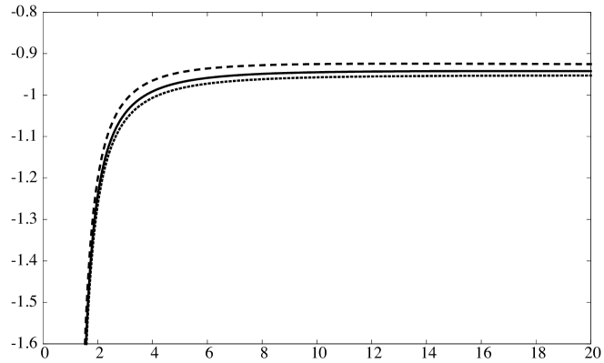
Figure 2: Scalar self-force acting on a particle of charge $q$ at position $r$ in the five-dimensional Schwarzschild-Tangherlini spacetime. The self-force is divided by the absolute value of the asymptotic expression of Eq. (142), and it is plotted as a function of $r/R$ for $\tilde{s}=10^{-4}$ (long-dashed curve), $\tilde{s}=10^{-6}$ (solid curve), and $\tilde{s}=10^{-8}$ (short-dashed curve).

The expansion of $g_{0}:=f^{3/2}F_{\rm poly}$ in powers of $x$ can be summed to a closed-form expression. The required steps are very similar to those followed in the electromagnetic case. Letting $s_{0}(p)$ be the sequence of coefficients associated with $g_{0}$, so that $g_{0}=\sum_{p=1}^{\infty}s_{0}(p)x^{p-1}$, we find that the manipulations $s_{1}(p)=(p-1)(p-2)s_{0}(p)$, $s_{2}(p):=s_{1}(p+1)-s_{1}(p)$, and $s_{3}(p):=s_{2}(p+1)-s_{2}(p)$ reveal a recognizable pattern,

$$s_{3}(p)=\frac{135}{23}\frac{(2p)!}{2^{2p}p!(p+3)!}.$$ (138)

The associated function is

$$g_{3}=-\frac{9}{46x^{4}}(5x^{3}-30x^{2}+40x-16)-\frac{72}{23x^{4}}(1-x)^{5/2},$$ (139)

and the original function $g_{0}$ is easily reconstructed. We find

$$f^{3/2}F_{\rm poly}=\frac{1}{92}\biggl{(}\frac{48}{x^{2}}-\frac{72}{x}+146-77x\biggr{)}-\frac{3}{23}\biggl{(}\frac{4}{x^{2}}-\frac{4}{x}+3\biggr{)}\sqrt{f}+\frac{9}{23}(2-x)\ln\frac{1+\sqrt{f}}{2\sqrt{f}}.$$ (140)

With this we finally arrive at

$$F =\frac{q^{2}R^{4}}{384r^{7}}\frac{\Xi}{f^{3/2}},$$ (141a)

$$\Xi =\frac{48}{x^{2}}-\frac{72}{x}+146-77x-12\biggl{(}\frac{4}{x^{2}}-\frac{4}{x}+3\biggr{)}\sqrt{f}+36(2-x)\ln\frac{\tilde{s}x(1+\sqrt{f})}{8\sqrt{f}},$$ (141b)

a closed-form expression for the scalar self-force acting on a particle of charge $q$ at a fixed radial position $r$ in the five-dimensional Schwarzschild-Tangherlini spacetime. We recall that $f=1-x$, and $\tilde{s}:=s/R$ is a dimensionless version of the averaging radius introduced in the Hadamard regularization prescription.

For $r/R\gg 1$, $\Xi=72\ln(\tilde{s}x/4)+O(1)$, and the self-force behaves as $F\sim F_{\rm asymp}$ with

$$F_{\rm asymp}=-\frac{3}{8}\frac{q^{2}R^{4}}{r^{7}}\ln\frac{2r}{\sqrt{\tilde{s}}R}$$ (142)

The self-force is attractive at large $r$, and it scales as $R^{4}\ln r/r^{7}$, which can be contrasted with the $R^{2}/r^{5}$ scaling of the electromagnetic self-force. As seen in Fig. 2, the self-force stays attractive as $r$ decreases toward $R$. Near the horizon, taking $r/R>1+\tilde{s}$, we find that the self-force is bounded by

$$F>-\frac{3}{128\sqrt{2}}\frac{q^{2}}{R^{3}}\frac{1}{\tilde{s}^{3/2}}\ln\frac{128}{\tilde{s}},$$ (143)

the same expression (5) that was found in the case of the electromagnetic self-force.

Appendix A Spherical harmonics in higher dimensions

We collect some useful results from the literature hochstadt:86 ; frye-efthimiou:12 pertaining to the theory of spherical harmonics in higher dimensions. The functions are defined on a unit $n$-sphere, with $n$ denoting the number of angular directions on the sphere. The spherical polar coordinates on the sphere are collectively denoted $\theta^{A}$, with the index $A$ running from 1 to $n$. Their relation to Cartesian coordinates $x^{a}$ in a Euclidean $(n+1)$-dimensional space is given by $x^{a}=r\Omega^{a}(\theta^{A})$, where $r$ is the distance to the origin and $\bm{\Omega}$ a unit vector in the direction of $\bm{x}$. The metric on the unit $n$-sphere is denoted $\Omega_{AB}$, and its inverse is $\Omega^{AB}$. The area element on the sphere is $d\Omega_{n}:=\sqrt{\Omega}\,d^{n}\theta$, with $\Omega:=\mbox{det}[\Omega_{AB}]$, and the integrated area is

$$\Omega_{n}:=\int d\Omega_{n}=\frac{2\pi^{(n+1)/2}}{\Gamma(\frac{n+1}{2})}.$$ (144)

The covariant derivative operator compatible with the metric is denoted $D_{A}$.

A.1 Definition and properties

The scalar harmonics $Y^{\ell,j}$ are defined in such a way that the function $a:=r^{\ell}Y^{\ell,j}(\theta^{A})$ satisfies Laplace’s equation $\nabla^{2}a=0$ in the $(n+1)$-dimensional space. The transformation to the spherical coordinates allows us to write

$$\nabla^{2}a=\partial_{rr}a+\frac{n}{r}\partial_{r}a+\frac{1}{r^{2}}D^{2}a,$$ (145)

with $\partial_{r}$ indicating partial differentiation with respect to $r$, and $D^{2}:=\Omega^{AB}D_{A}D_{B}$ denoting the Laplacian operator on the unit $n$-sphere. Making the substitution produces the eigenvalue equation

$$\bigl{[}D^{2}+\ell(\ell+n-1)\bigr{]}Y^{\ell,j}=0$$ (146)

for the spherical harmonics. Here $\ell=0,1,2,\cdots$, and the index $j$ runs over a number $N(n,\ell)$ of linearly independent functions, with

$$N(n,\ell)=\frac{(2\ell+n-1)(\ell+n-2)!}{(n-1)!\ell!}.$$ (147)

For $n=2$ we have the familiar $N(2,\ell)=2\ell+1$, and for $n=3$ we have $N(3,\ell)=(\ell+1)^{2}$.

Spherical harmonics of a given degree $\ell$ can be orthonormalized by implementing the Gram-Schmidt procedure, while spherical harmonics of different degrees are necessarily orthogonal. The orthonormality relations are

$$\int\bar{Y}^{\ell,j}(\bm{\Omega})Y^{\ell^{\prime},j^{\prime}}(\bm{\Omega})\,d\Omega_{n}=\delta_{\ell\ell^{\prime}}\delta_{jj^{\prime}},$$ (148)

with an overbar indicating complex conjugation. Here and below we use the direction $\bm{\Omega}$ as a convenient encoding of the angles $\theta^{A}$.

Any function $b$ of the angular coordinates $\theta^{A}$ can be decomposed in spherical harmonics, according to

$$b(\bm{\Omega})=\sum_{\ell=0}^{\infty}\sum_{j=0}^{N-1}b_{\ell,j}Y^{\ell,j}(\bm{\Omega}),$$ (149)

with coefficients given by

$$b_{\ell,j}=\int f(\bm{\Omega})\bar{Y}^{\ell,j}(\bm{\Omega})\,d\Omega_{n}.$$ (150)

These relations imply the completeness relation

$$\sum_{\ell j}\bar{Y}^{\ell,j}(\bm{\Omega^{\prime}})Y^{\ell,j}(\bm{\Omega})=\delta(\bm{\Omega},\bm{\Omega^{\prime}}),$$ (151)

in which $\delta(\bm{\Omega},\bm{\Omega^{\prime}})$ is a scalarized delta function defined by

$$\int\delta(\bm{\Omega},\bm{\Omega^{\prime}})b(\bm{\Omega^{\prime}})\,d\Omega^{\prime}_{n}=b(\bm{\Omega}).$$ (152)

A.2 Axisymmetric mode

Let $\chi:=\theta^{n}$ be the angle from the polar axis, and let the metric on the unit $n$-sphere be expressed as

$$d\Omega_{n}^{2}=d\chi^{2}+\sin^{2}\chi\,d\Omega^{2}_{n-1},$$ (153)

where $d\Omega^{2}_{n-1}$ is the metric on a unit $(n-1)$-sphere. We denote by $Y^{\ell,0}$ the spherical harmonic of degree $\ell$ that depends on $\chi$ only, and we call this function the axisymmetric mode. Its eigenvalue equation takes the form of the ordinary differential equation

$$\frac{d^{2}Y^{\ell,0}}{d\chi^{2}}+(n-1)\frac{\cos\chi}{\sin\chi}\frac{dY^{\ell,0}}{d\chi}+\ell(\ell+n-1)Y^{\ell,0}=0,$$ (154)

and the transformation $u=\cos\chi$ brings this to the form of a generalized Legendre equation

$$(1-u^{2}){\cal P}^{\prime\prime}_{\ell}-nu{\cal P}^{\prime}_{\ell}+\ell(\ell+n-1){\cal P}_{\ell}=0,$$ (155)

in which a prime indicates differentiation with $u$. The generalized Legendre functions are defined by the generating function

$$g:=(1-2ut+t^{2})^{-\frac{1}{2}(n-1)}=\sum_{\ell}a_{\ell}{\cal P}_{\ell}(u)t^{\ell},$$ (156)

where

$$a_{\ell}:=\biggl{(}\begin{array}[]{c}\ell+n-2\\ \ell\end{array}\biggr{)}=\frac{(\ell+n-2)!}{(n-2)!\,\ell!}.$$ (157)

When $n=2$, $a_{\ell}=1$, and we recover the usual definition of the Legendre polynomials. When $x=1$ we have that $g=(1-t)^{-(n-1)}$, with a series expansion given by $\sum_{\ell}a_{\ell}t^{\ell}$; this ensures that

$${\cal P}_{\ell}(1)=1.$$ (158)

The axisymmetric mode $Y^{\ell,0}(\chi)$ and the generalized Legendre function ${\cal P}_{\ell}(\cos\chi)$ differ by a normalization factor that reconciles Eq. (148) with Eq. (158); the relation is

$$Y^{\ell,0}(\chi)=\sqrt{\frac{N(n,\ell)}{\Omega_{n}}}{\cal P}_{\ell}(\cos\chi).$$ (159)

A.3 Value on the polar axis

Suppose that in Eq. (151), the unit vector $\bm{\Omega^{\prime}}$ is aligned with the polar axis $\bm{e}$. The completeness relation becomes

$$\delta(\bm{\Omega},\bm{e})=\sum_{\ell j}\bar{Y}^{\ell,j}(\bm{e})Y^{\ell,j}(\bm{\Omega}),$$ (160)

and since $\delta(\bm{\Omega},\bm{e})$ is axisymmetric relative to $\bm{e}$, we must have that only the $j=0$ term contributes to the sum. This implies that $\bar{Y}^{\ell,j}(\bm{e})=\bar{Y}^{\ell,0}(\bm{e})\delta_{j0}$, and since $\bar{Y}^{\ell,0}(\bm{e})=\sqrt{N(n,\ell)/\Omega_{n}}{\cal P}_{\ell}(1)=\sqrt{N(n,\ell)/\Omega_{n}}$, we have that

$$Y^{\ell,j}(\bm{e})=\sqrt{\frac{N(n,\ell)}{\Omega_{n}}}\delta_{j0}.$$ (161)

Making the substitution in $\delta(\bm{\Omega},\bm{e})$, we arrive at

$$\delta(\bm{\Omega},\bm{e})=\sum_{\ell}\frac{N(n,\ell)}{\Omega_{n}}{\cal P}_{\ell}(\cos\chi),$$ (162)

where $\cos\chi=\bm{\Omega}\cdot\bm{e}$.

References

- (1) A. G. Smith and C. M. Will, Force on a static charge outside a Schwarzschild black hole, Phys. Rev. D 22, 1276 (1980).
- (2) L. M. Burko, Y. T. Liu, and Y. Soen, Self-force on charges in the spacetime of spherical shells, Phys. Rev. D 63, 024015 (2000), arXiv:gr-qc/0008065.
- (3) W. Unruh, Self force on charged particles, Proc. Roy. Soc. London A348, 447 (1976).
- (4) K. Shankar and B. F. Whiting, Self force of a static electric charge near a Schwarzschild Star, Phys. Rev. D 76, 124027 (2007), arXiv:0707.0042.
- (5) T. D. Drivas and S. E. Gralla, Dependence of Self-force on Central Object, Class. Quantum Grav. 28, 145025 (2011), arXiv:1009.0504.
- (6) S. Isoyama and E. Poisson, Self-force as probe of internal structure, Class. Quantum Grav. 29, 155012 (2012), arXiv:1205.1236.
- (7) J. Kuchar, E. Poisson, and I. Vega, Electromagnetic self-force on a static charge in Schwarzschild–de Sitter spacetimes, Class. Quantum Grav. 30, 235033 (2013), arXiv:1307.8342.
- (8) V. P. Frolov and A. Zelnikov, Scalar and electromagnetic fields of static sources in higher dimensional Majumdar-Papapetrou spacetimes, Phys. Rev. D 85, 064032 (2012), arXiv:1202.0250.
- (9) V. P. Frolov and A. Zelnikov, Self-energy of a scalar charge near higher-dimensional black holes, Phys. Rev. D 85, 124042 (2012).
- (10) V. P. Frolov and A. Zelnikov, Classical self-energy and anomaly, Phys. Rev. D 86, 044022 (2012).
- (11) V. P. Frolov and A. Zelnikov, Anomaly and the self-energy of electric charges, Phys. Rev. D 86, 104021 (2012).
- (12) E. T. Copson, On electrostatics in a gravitational field, Proc. R. Soc. London A118, 184 (1928).
- (13) B. Linet, Electrostatics and magnetostatics in the Schwarzschild metric, J. Phys. A: Math. Gen. 9, 1081 (1976).
- (14) J. Hadamard, Lectures on Cauchy’s problem in linear partial differential equations (Yale University Press, New Haven, 1923).
- (15) A. G. Wiseman, Self-force on a static scalar test charge outside a Schwarzschild black hole, Phys. Rev. D 61, 084014 (2000), arXiv:gr-qc/0001025.
- (16) F. Tangherlini, Schwarzschild field in n dimensions and the dimensionality of space problem, Nuovo Cimento 27, 636 (1963).
- (17) M. Abramowitz and I. A. Stegun, Handbook of Mathematical Functions (Dover, New York, 1972).
- (18) T. C. Quinn and R. M. Wald, Axiomatic approach to electromagnetic and gravitational radiation reaction of particles in curved spacetime, Phys. Rev. D 56, 3381 (1997), arXiv:gr-qc/9610053.
- (19) L. Barack and A. Ori, Mode sum regularization approach for the self-force in black hole spacetime, Phys. Rev. D 61, 061502(R) (2000), arXiv:gr-qc/9912010.
- (20) L. Barack, Y. Mino, H. Nakano, A. Ori, and M. Sasaki, Calculating the gravitational self-force in Schwarzschild spacetime, Phys. Rev. Lett. 88, 091101 (2002), arXiv:gr-qc/0111001.
- (21) L. Barack and A. Ori, Regularization parameters for the self-force in Schwarzschild spacetime. II. Gravitational and electromagnetic cases, Phys. Rev. D 67, 024029 (2003), arXiv:gr-qc/0209072.
- (22) B. S. DeWitt and R. W. Brehme, Radiation damping in a gravitational field, Ann. Phys. (N.Y.) 9, 220 (1960).
- (23) F. G. Friedlander, The wave equation on a curved spacetime (Cambridge University Press, Cambridge, 1975).
- (24) E. Poisson, A. Pound, and I. Vega, The motion of point particles in curved spacetime, Living Rev. Rel. 14, 7 (2011), arXiv:1102.0529.
- (25) J. L. Synge, Relativity: The General Theory (North-Holland, Amsterdam, 1960).
- (26) R. Haas and E. Poisson, Mode-sum regularization of the scalar self-force: Formulation in terms of a tetrad decomposition of the singular field, Phys. Rev. D 74, 044009 (2006), arXiv:gr-qc/0605077.
- (27) S. Detweiler, E. Messaritaki, and B. F. Whiting, Self-force of a scalar field for circular orbits about a Schwarzschild black hole, Phys. Rev. D 67, 104016 (2003), arXiv:gr-qc/0205079.
- (28) I. S. Gradshteyn and I. M. Ryzhik, Table of Integrals, Series, and Products (Academic Press, Orlando, 1980).
- (29) H. Hochstadt, The functions of mathematical physics (Dover Publications, New York, 1986).
- (30) C. R. Frye and C. J. Efthimiou, Spherical Harmonics in p Dimensions (2012), arXiv:1205.3548.