Front propagation in cellular flows for fast reaction and small diffusivity

Abstract

We investigate the influence of fluid flows on the propagation of chemical fronts arising in FKPP type models. We develop an asymptotic theory for the front speed in a cellular flow in the limit of small molecular diffusivity and fast reaction, i.e., large Péclet (Pe) and Damköhler (Da) numbers. The front speed is expressed in terms of a periodic path – an instanton – that minimizes a certain functional. This leads to an efficient procedure to calculate the front speed, and to closed-form expressions for $(\log\text{Pe})^{-1}\ll\text{Da}\ll\text{Pe}$ and for $\text{Da}\gg\text{Pe}$. Our theoretical predictions are compared with (i) numerical solutions of an eigenvalue problem and (ii) simulations of the advection–diffusion–reaction equation.

The spreading of chemical or biological populations in fluid flows is a fundamental problem in many areas of science and engineering with applications ranging from plankton blooms to combustion Tel et al. (2005); Neufeld and Hernández-Garcia (2009). In the absence of flow, this spreading results from the competition between spatial diffusion, local growth and saturation, and leads to the formation of wave fronts that travel undeformed at constant speed Murray (2002). A number of theoretical results describe the influence that divergence-free, spatially smooth flows have on such fronts (see Xin (2000a, b) for comprehensive reviews). These have stimulated experiments using a variety of reactions and flow configurations Leconte et al. (2003); Paoletti et al. (2006); Schwartz and Solomon (2008), with much effort devoted to steady spatially periodic cellular flows Paoletti and Solomon (2005); Pocheau and Harambat (2006, 2008); Thompson et al. (2010).

Using the classic model of Fisher Fisher (1937) and Kolmogorov et al. Kolmogorov et al. (1937) (FKPP) based on logistic-type growth, Gärtner and Freidlin (1979) showed that the speed of the pulsating front that arises in such periodic flows can be obtained by solving an eigenvalue problem (see below). In practice, this procedure requires rather involved numerical computations; there is therefore a need for simplified results that provide scaling predictions or closed-form expressions in asymptotic regimes. Results of this type have been derived in the limit of slow reactions and small diffusivity Audoly et al. (2000); Novikov and Ryzhik (2007). Here we consider the opposite limit of fast reaction (e.g. Majda and Sougadinis (1994)) relevant, for instance, to premixed flame propagation Peters (2000). In this limit, we obtain a compact expression for the speed in terms of a single periodic path that minimizes an action functional. This brings new physical insight, in particular into the role of the flow’s stagnation points, and yields new closed-form results valid for a remarkably large range of reaction rates. It also provides an efficient way to compute the speed in a regime where direct numerical computations are most challenging because of the widely disparate spatial scales (see e.g. Fig. 1).

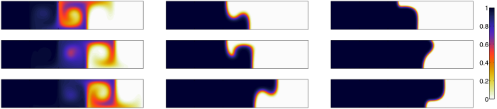
Figure 1: (Color online). Successive snapshots of the concentration $\theta$ for $\text{Pe}=50$ and $\text{Da}=0.5$ (left), $\text{Da}=5$ (middle), and $\text{Da}=20$ (right) with time increasing from the top to the bottom rows. The corresponding front speeds are $c\approx 0.5$, $c\approx 1$, and $c\approx 1.6$.

Model.—The effect of a background flow $\bm{u}$ is incorporated in the FKPP advection–diffusion–reaction equation

$$\partial_{t}\theta+\bm{u}\cdot\nabla\theta=\text{Pe}^{-1}\Delta\theta+\text{Da}\,r(\theta),$$ (1)

for the population concentration $\theta$. Here, the reaction term is $r(\theta)=\theta(1-\theta)$ or, more generally, any function $r(\theta)$ that satisfies $r(0)=r(1)=0$ with $r(\theta)>0$ for $\theta\in(0,1)$, $r(\theta)<0$ for $\theta\notin[0,1]$ and $r^{\prime}(0)=\sup_{0<\theta<1}r(\theta)/\theta=1$. The non-dimensional parameters are the Péclet and Damköhler numbers $\text{Pe}=U\ell/\kappa$ and $\text{Da}=\ell/(U\tau)$ where $U$ and $\ell$ are the characteristic amplitude and lengthscale of the flow, $\kappa$ the molecular diffusivity, and $\tau$ the reaction time. We consider the two-dimensional cellular flow $\bm{u}=(u_{1},u_{2})=(-\partial_{y}\psi,\partial_{x}\psi)$ with streamfunction

$$\psi(x,y)=-\sin x\sin y.$$ (2)

We take the domain to be the strip $D=(-\infty,\infty)\times[0,\pi]$ along which an infinite array of identical cells are arranged, each of which composed of two half-cells of opposite circulation with hyperbolic stagnation points at each corner (streamlines are shown for a single cell in Fig. 2). As initial condition we take $\theta(x,y,0)=\Theta(-x)$, where $\Theta$ is the Heaviside step function. The boundary conditions are $\theta(\infty,y,t)=0$ and $\theta(-\infty,y,t)=1$, so that the front advances rightwards, and no flux, $\partial_{y}\theta=0$ at $y=0,\,\pi$. The front characteristics change drastically with Da. When Da is small, the front’s leading edge is confined near the cell boundaries (see left column in Fig. 1). As Da increases, the front sharpens and the imprint of the flow, the boundary-layer structure in particular, is less prominent (see middle and right columns in Fig. 1).

The long-time speed of propagation of the front is determined by the behavior of the solution near the front’s leading edge, where $0<\theta\ll 1$ and $r(\theta)\approx r^{\prime}(0)\theta=\theta$. For steady periodic flows such as (2), this is given by

$$c=\inf_{q>0}\frac{f(q)+\text{Da}}{q},$$ (3)

where $f(q)$ is the largest eigenvalue of

$$\mathcal{L}v=f(q)v,$$ (4a)

with the operator $$\mathcal{L}$$ defined by

$$\mathcal{L}=\text{Pe}^{-1}\Delta-\bm{u}\cdot\nabla-2\text{Pe}^{-1}q\partial_{x}+(u_{1}q+\text{Pe}^{-1}q^{2}),$$ (4b)

and periodic and no-flux boundary conditions in $x$ and $y$, respectively [15, 20, Ch. 7, 21]. This result is intimately connected with the long-time large-deviation rate function associated with the concentration of the non-reacting passive scalar (i.e., $\text{Da}=0$); specifically, $f(q)$ is the Legendre transform of this rate function Gärtner and Freidlin (1979); Freidlin (1985); Haynes and Vanneste (2014); Tzella and Vanneste .

In the absence of a background flow, $f(q)=q^{2}/\text{Pe}$, recovering the classical formula for the bare speed $c_{0}=2\sqrt{\text{Da}/\text{Pe}}=2\sqrt{\kappa/\tau}$ (see Refs. Fisher (1937); Kolmogorov et al. (1937); Leach and Needham (2003); van Saarloos (2003) and references therein). For general $\bm{u}\neq 0$, the eigenvalue problem (3)–(4) cannot be solved explicitly.

Small diffusivity, fast reaction.—Our purpose is to use asymptotic analysis to obtain the speed of the front in the large-Péclet limit with

$$\gamma=\text{Da}/\text{Pe}=O(1),$$

corresponding to the geometric optics regime defined by $\kappa,\tau\to 0$ with $\kappa/\tau=O(1)$ Williams (1985). This can be achieved by analyzing the large-Pe limit of the eigenvalue problem (4), or by considering the large-$t$ limit of the geometric optics theory treatment of (Freidlin, 1985, Ch. 6) (see also Majda and Sougadinis (1994); Freidlin and Sowers (1999)). It is however convenient to start with the basic result exploited by Gärtner and Freidlin (1979); Freidlin (1985), namely that the front speed is controlled by the point at which the solution to the linearization of equation (1) neither grows nor decays.

We seek a solution to this equation in the WKB form

$$\theta(x,y,t)\sim\exp(-\text{Pe}(I(x,y,t)-\gamma t)),\quad\text{for $\text{Pe}\gg 1$},$$ (5)

where $I(x,y,t)$ can be recognized as the small-noise large-deviation rate function Freidlin and Wentzell (1998). At leading-order, $\partial_{t}I+H(\nabla I,x,y)=0$, where $H=\lVert\nabla I\rVert^{2}+\bm{u}(x,y)\cdot\nabla I$ is the Hamiltonian and $\lVert\cdot\rVert$ the usual norm. Its solution is well known from Hamilton–Jacobi theory (e.g., Evans (2010); Freidlin and Wentzell (1998)) and given by

$$I(x,y,t)=\frac{1}{4}\inf_{\bm{\phi}(\cdot)}\int_{0}^{t}\lVert\dot{\bm{\phi}}(s)-\bm{u}(\bm{\phi}(s))\rVert^{2}ds,$$ (6)

subject to $\bm{\phi}(t)=(x,y)$ and $\bm{\phi}(0)=(0,\cdot)$. Thus, the behavior of (5) is controlled by a single path $\bm{\phi}^{\ast}(s)$ that minimizes this integral. This optimal path is often called instanton Dykman et al. (1994). Expression (5) then indicates that for $t\gg 1$, the front speed satisfies

$$\gamma=\lim_{t\to\infty}\frac{I(ct,y,t)}{t}\equiv\mathscr{G}(c),$$ (7)

where the limit $t\to\infty$ eliminates the dependence on $y$. This leads to

$$c=\mathscr{G}^{-1}(\gamma).$$ (8)

The front speed is therefore obtained by calculating $\mathscr{G}(c)$. This calculation is significantly simplified by observing that the limit in (7) is determined in terms of periodic trajectories, an observation justified rigorously in Piatnitski (1998). We take solutions $\bm{\phi}(s)$ to be periodic in the sense that $\bm{\phi}(\tau)=\bm{\phi}(0)+(2\pi,0)$, where the period is $\tau=2\pi/c$. Letting $\sigma=cs$, we obtain the simplified expression

$$\mathscr{G}(c)=\frac{1}{8\pi}\inf_{\bm{\phi}(\cdot)}\int_{0}^{2\pi}\lVert c{\bm{\phi}}^{\prime}(\sigma)-\bm{u}(\bm{\phi}(\sigma))\rVert^{2}d\sigma,$$ (9)

subject to $\bm{\phi}(2\pi)=\bm{\phi}(0)+(2\pi,0)$. Expressions (8) and (9) are the main result of the paper. They provide a direct way of computing the instantons and thus the front speed. Note that $\mathscr{G}(c)$ may be interpreted as the Legendre transform of $\overline{H}$, the effective Hamiltonian of the homogenized Hamilton–Jacobi equation $\partial_{t}I+\overline{H}(\nabla I)=0$ Lions et al. ; Majda and Sougadinis (1994). In order to derive (8), we have formally assumed that $\gamma=O(1)$. However, the asymptotic results apply over a broad range of values of $\gamma$, specifically $\gamma\gg(\text{Pe}\log\text{Pe})^{-1}$ as we show below.

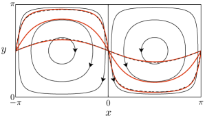
Figure 2: (Color online). Streamlines of the cellular flow with streamfunction (2) (thin solid black lines) and trajectories of the instantons minimising (9) (thick red lines). The instantons are calculated numerically for $c=0.5$ (corresponding to $\gamma\approx 0.002$), $c=1$, ($\gamma\approx 0.09$) and $c=5$ ($\gamma\approx 5.9$) and become closer to the straight line $y=\pi/2$ as $c$ increases. The dashed lines show the small-$c$ and large-$c$ asymptotic approximations obtained using (10) for $c=0.5$ and (15) for $c=5$, respectively.

The solution to the minimization problem (9) is easy to obtain numerically. We first discretize (9) and use MATLAB to minimize the action. We iterate over $c$, starting with large values for which the straight line $\bm{\phi}^{\ast}(s)=(cs,\pi/2)$ is a good initial guess. Characteristic examples of instantons obtained for different values of $c$ are shown in Fig. 2 (the two cases with $c=0.5$ and $c=1$ correspond to the first two columns in Fig. 1). For large values of $c$, the instanton is close to a straight line. For small values of $c$, it follows closely a streamline near the cell boundaries. Figure 3 shows the behaviour of $c$ as a function of $\gamma$ deduced from (8).

Asymptotic limits.—We now obtain closed-form expressions for the speed $c$ in two asymptotic limits. The first one corresponds to $\gamma\ll 1$ and hence $c\ll 1$. Numerical results (see Fig. 2 for $c=0.5$) suggest that the instanton departs from the streamline only for $y\approx\pi/2$ when it crosses the separatrix between adjacent cells. It is also clear that (9) is minimized when $\bm{\phi}^{\ast}(\sigma)=(x(\sigma),y(\sigma))$ satisfies $cy^{\prime}\approx-\cos x\sin y$ (so that the instanton and flow speeds differ only in the $x$-direction). Exploiting symmetry to consider $0\leq\sigma\leq\pi/2$ only, with $x(0)=0$, $y(0)=x(\pi/2)=\pi/2$ and $y^{\prime}(\pi/2)=0$, we divide the instanton into two regions (see Fig. 2). In region $1$, where $x\ll 1$, the integrand in (9) is approximately $(cx^{\prime}-x\cos y)^{2}$, leading to the Euler–Lagrange equation $c^{2}x^{\prime\prime}=x$ (since $cy^{\prime}\approx-\sin y$). In region $2$, $y\ll 1$, $cx^{\prime}=\sin x\cos y\approx-\sin x$ and $cy^{\prime}=-\cos x\sin y\approx-y\cos x$. Matching the solutions for $x,y\ll 1$ (the cell corner) gives the approximation

$$\bm{\phi}^{\ast}(\sigma)\sim\begin{cases}\left({C}_{1}(\sigma),{C}_{2}(\sigma)\right)&\text{for }\sigma\ll\pi/2\\ \left({C}_{2}(\pi/2-\sigma),{C}_{3}(\pi/2-\sigma)\right)&\text{for }\sigma\gg c\end{cases}$$ (10)

where

$$C_{1}(\sigma) =4\exp\left({-\frac{\pi}{2c}}\right)\sinh\left(\frac{\sigma}{c}\right),$$

$$C_{2}(\sigma) =2\tan^{-1}\left(\exp\left(-\frac{\sigma}{c}\right)\right),$$

$$C_{3}(\sigma) =4\exp\left(-\frac{\pi}{2c}\right)\cosh\left(\frac{\sigma}{c}\right).$$

Expression (10) is in very good agreement with our numerical solution (see Fig. 2 for $c=0.5$).

\begin{overpic}[scale={.29}]{speed_asym6.pdf} \put(52.0,9.0){\includegraphics[scale={0.15}]{speed_asym_loglin3.pdf}} \end{overpic}

Figure 3: Front speed $c$ for $\text{Pe}\gg 1$ as a function of $\gamma$. Prediction (8) derived from the numerical minimization of (9) (solid black line) is compared with its small-$c$ approximation (12) (lower dashed line), its large-$c$ approximation (16) (upper dashed line), and the bare speed $c_{0}=2\sqrt{\gamma}$ (dotted line). The inset focuses on smaller values of $\gamma$.

Using (10) gives the integrand in (9) as $(cx^{\prime}-x\cos y)^{2}\approx 16\exp\left(-\pi/c\right)\cosh^{-2}\left(\sigma/c\right)$, leading to

$$\mathscr{G}(c)\sim 4\times(2/\pi)ce^{-\pi/c},\quad\text{where $c\ll 1$}$$ (11)

and the factor $4$ appears because, for $\sigma\in[0\,\,2\pi]$, there are $4$ regions that are similar to region $1$. Inverting (11) and using (8) finally gives

$$c\sim\frac{\pi}{W_{p}(8\gamma^{-1})},\quad\text{for $\gamma\ll 1$,}$$ (12)

where $W_{p}$ denotes the principal real branch of the Lambert $W$ function NIS . This approximation holds for $(\log\text{Pe})^{-1}\ll\text{Da}\ll\text{Pe}$: the lower bound follows from requiring that the argument of the exponential in (5) be large, $\text{Pe}\,I\sim\text{Da}\,\tau\gg 1$, where the period is roughly estimated as $\tau=2\pi/c\sim\log\text{Pe}/2$ (see (13) below and Tzella and Vanneste for a complete argument). Figure 3 shows that this approximation is excellent within its range of validity. Since $\gamma\ll 1$, it is consistent to approximate $W_{p}(8\gamma^{-1})$ to reduce (12) to

$$c\approx\frac{\pi}{\log\text{Pe}}.$$ (13)

A qualitatively similar expression was obtained in Abel et al. (2002); Cencini et al. (2003) using a heuristic approach based on the so-called G-equation. To our knowledge, no equivalent expression to (13) has previously been derived from the FKPP equation (1). Note that the logarithmic dependence of the speed on Pe and its slow growth with Da (captured by (12) but not (13)) is associated with the holdup of the instanton near the hyperbolic stagnation points at the cell corners.

The second limit leading to closed-form results corresponds to $\gamma\gg 1$, hence $c\gg 1$. In this case, we seek an instanton as a power series $\bm{\phi}^{\ast}(\sigma)=(\sigma,y_{0})+c^{-1}(x_{1}(\sigma),y_{1}(\sigma))+\ldots$, where $x_{1}$, $y_{1}$ are functions of period $2\pi$ that satisfy $x_{1}(0)=y_{1}(0)=0$. Substituting into (9), we find that at $O(c^{-1})$,

$$\mathscr{G}(c)=\frac{c^{2}}{4}+\frac{1}{8\pi}\inf_{x_{1},y_{0},y_{1}}\int_{0}^{2\pi}(x_{1}^{\prime 2}+y_{1}^{\prime 2}+4y_{1}\sin\sigma\sin y_{0})d\sigma,$$ (14)

after some manipulations. Minimizing this integral leads to the instanton

$$\bm{\phi}^{\ast}(\sigma)=\left(\sigma,\frac{\pi}{2}\right)+c^{-1}(0,-2\sin\sigma)+\ldots,\quad\text{for $c\gg 1$,}$$ (15)

in excellent agreement with our numerical solution (see Fig. 2 for $c=5$). Combining (14) and (15), yields $\mathscr{G}(c)=c^{2}/4-3/8+O(c^{-2})$. We now use (8) to find that

$$c\sim 2\sqrt{\gamma}\left(1+\frac{3}{16\gamma}+\ldots\right),\quad\text{for $\gamma\gg 1$,}$$ (16)

which corresponds to $\text{Da}\gg\text{Pe}$. The leading-order term in (16) is the bare speed $c_{0}$. As Fig. 3 shows, the second term in the expansion is necessary for a good agreement between asymptotic and full results.

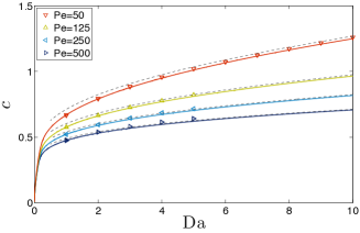
Figure 4: (Color online). Front speed $c$ as a function of Da for different values of Pe. The large-Pe prediction (8) derived from the numerical minimization of (9) (dashed lines) is compared with the exact expression (3) estimated by solving the eigenvalue problem (4) numerically (solid lines) and with direct numerical simulations of (1) (symbols).

Comparison with numerical results. We now compare our predictions for $c$ derived from (8)–(9) with values obtained from (i) numerical evaluation of the principal eigenvalue in (4), and (ii) direct numerical simulations of (1) with $r(\theta)=\theta(1-\theta)$. For (i) we use a standard second-order discretization to approximate (4) and choose the spatial resolution $\Delta$ to satisfy $\pi/\Delta=750$. The resulting matrix eigenvalue problem is solved for a range of values of $q$ using MATLAB. For (ii) we discretize (1) using a fractional-step method with a Godunov splitting which alternates between advection (using a first-order upwind method with a minmod limiter – see Leveque (2002) for details), diffusion (using an alternating direction implicit method) and reaction (solved exactly). We choose the same spatial resolution $\Delta$ as for (4). The computational domain is made finite using artificial boundaries at $x=\pm N\pi$, with $N=5$, so that boundary effects are negligible. The front is tracked for long times by modifying the computational domain: when the solution at $x=(N-1)\pi$ exceeds $\delta=10^{-6}$, we eliminate the nodes with $-N\pi\leqslant x\leqslant(-N+1)\pi$ and add new nodes with $N\pi\leqslant x\leqslant(N+1)\pi$ where we set $\theta=0$. We calculate the front speed using a linear fit of the right endpoint of the front, $x^{+}_{\epsilon}(t)=\text{max}\{x:\theta(x,t)=\epsilon\}$ where $\epsilon=10^{-3}$. Results are insensitive to the exact values of $\epsilon$ and $\delta$.

The three set of numerical results are shown in Fig. 4. The speeds derived from the eigenvalue equation (4) are in excellent agreement with the corresponding values obtained from the full numerical simulations of equation (1). With increasing values of Pe, the asymptotic expression (8)–(9) becomes increasingly accurate, with excellent agreement for $\text{Pe}=250,500$ and satisfactory agreement for the moderate values $\text{Pe}=50,125$. As expected, (8)–(9) is valid for a broad range of values of Da, restricted only by $\text{Da}\gg(\log\text{Pe})^{-1}$. Note that the use of both the eigenvalue equation and the full numerical simulations is restricted: as Pe increases, the solutions to (1) and (4) become progressively localized, with $O(1/\sqrt{\text{Da}\text{Pe}}$) lengthscales that are challenging to resolve when $\text{Da},\,\text{Pe}\gg 1$.

Conclusion.—We have derived a compact expression for the front speed based on the minimization of the large-deviation action (9) over periodic instantons. This leads to the efficient computation of the speed for a large range of values of Da. For the particular case of cellular flows, this expression provides the new closed-form results (12) and (16) valid for $(\log\text{Pe})^{-1}\ll\text{Da}\ll\text{Pe}$ and $\text{Da}\gg\text{Pe}$. In the first regime, the passage of the front near the stagnation points at the cell corners is shown to control the front speed; as a result this is almost insensitive to the reaction rate and depends logarithmically on the Péclet number. For $\text{Da}=O(\log\text{Pe})^{-1}$ and smaller, the front speed is not controlled by a single minimizing trajectory, and asymptotic solutions to the eigenvalue problem (4) must be sought by other means; this will be the subject of future work (Tzella and Vanneste, ).

The authors thank P. H. Haynes, G. C. Papanicolaou and A. Pocheau for helpful discussions. The work was supported by EPSRC (Grant No. EP/I028072/1).

References

- Tel et al. (2005) T. Tel, A. de Moura, C. Grebogi, and G. Károlyi, Phys. Rep. 413, 91 (2005).
- Neufeld and Hernández-Garcia (2009) Z. Neufeld and E. Hernández-Garcia, Chemical and Biological Processes in Fluid Flows: A Dynamical Systems Approach (Imperial College Press, 2009).
- Murray (2002) J. Murray, Mathematical Biology I: An introduction (Springer-Verlag, 3rd edition, 2002).
- Xin (2000a) J. Xin, SIAM Rev. 42, 161 (2000a).
- Xin (2000b) J. Xin, An introduction to fronts in random media (Springer, 2000).
- Leconte et al. (2003) M. Leconte, J. Martin, N. Rakotomalala, and D. Salin, Phys. Rev. Lett. 90, 128302 (2003).
- Paoletti et al. (2006) M. S. Paoletti, C. R. Nugent, and T. H. Solomon, Phys. Rev. Lett. 96, 124101 (2006).
- Schwartz and Solomon (2008) M. E. Schwartz and T. H. Solomon, Phys. Rev. Lett. 100, 028302 (2008).
- Paoletti and Solomon (2005) M. S. Paoletti and T. H. Solomon, Phys. Rev. E 72, 046204 (2005).
- Pocheau and Harambat (2006) A. Pocheau and F. Harambat, Phys. Rev. E 73, 065304 (2006).
- Pocheau and Harambat (2008) A. Pocheau and F. Harambat, Phys. Rev. E 77, 036304 (2008).
- Thompson et al. (2010) B. W. Thompson, J. Novak, M. C. T. Wilson, M. M. Britton, and A. F. Taylor, Phys. Rev. E 81, 047101 (2010).
- Fisher (1937) R. Fisher, Ann. Eugenics 7, 355 (1937).
- Kolmogorov et al. (1937) A. N. Kolmogorov, I. G. Petrovsky, and N. S. Piskunov, Bull. Univ. Moskov. Ser. Internat. Sect. 1, 1 (1937).
- Gärtner and Freidlin (1979) J. Gärtner and M. I. Freidlin, Soviet Math. Dokl. 20, 1282 (1979).
- Audoly et al. (2000) B. Audoly, H. Berestycki, and Y. Pomeau, C. R. Acad. Sci. Paris, t. 328, Série II b 328, 255 (2000).
- Novikov and Ryzhik (2007) A. Novikov and L. Ryzhik, Arch. Ration. Mech. An. 184, 23 (2007).
- Majda and Sougadinis (1994) A. J. Majda and O. E. Sougadinis, Nonlinearity 7, 1 (1994).
- Peters (2000) N. Peters, Turbulent combustion (Cambridge University Press, 2000).
- Freidlin (1985) M. Freidlin, Functional Integration and Partial Differential Equations, 260 (Princeton University Press, 1985).
- Evans and Souganidis (1989) L. Evans and P. Souganidis, Ann. I. H. Poincare-An. S6, 229 (1989).
- Haynes and Vanneste (2014) P. H. Haynes and J. Vanneste, J. Fluid Mech. 745, 321 (2014).
- (23) A. Tzella and J. Vanneste, “FKPP fronts in cellular flows: the large-Péclet regime.” In preparation.
- Leach and Needham (2003) J. Leach and D. Needham, Matched Asymptotic Expansions in Reaction-Diffusion Theory (Springer Monographs in Mathematics, 2003).
- van Saarloos (2003) W. van Saarloos, Phys. Rep. 386, 29 (2003).
- Williams (1985) F. A. Williams, The Mathematics of Combustion, edited by J. D. Buckmaster (SIAM, 1985) pp. 97–131.
- Freidlin and Sowers (1999) M. I. Freidlin and R. B. Sowers, Stochastic Processes and their Applications 82, 23 (1999).
- Freidlin and Wentzell (1998) M. Freidlin and A. D. Wentzell, Random Perturbations of Dynamical Systems, 260 (Springer, 1998).
- Evans (2010) C. L. Evans, Partial Differential Equations, Vol. 19 (American Mathematical Society, 2010).
- Dykman et al. (1994) M. I. Dykman, E. Mori, J. Ross, and P. M. Hunt, J. Chem. Phys. 100, 5735 (1994).
- Piatnitski (1998) A. Piatnitski, Commun. Math. Phys. 197, 527 (1998).
- (32) P. L. Lions, G. C. Papanicolaou, and S. Varadhan, “Homogenization of Hamilton–-Jacobi equations,” (unpublished).
- (33) “NIST digital library of mathematical functions,” http://dlmf.nist.gov/, Release 1.0.6 of 2013-05-06.
- Abel et al. (2002) M. Abel, M. Cencini, D. Vergni, and A. Vulpiani, Chaos 12, 481 (2002).
- Cencini et al. (2003) M. Cencini, A. Torcini, D. Vergni, and A. Vulpiani, Phys. Fluids 15, 679 (2003).
- Leveque (2002) R. J. Leveque, Finite Volume Methods for Hyperbolic Problems (Cambridge University Press, 2002).