Early ultraviolet emission in the Type Ia supernova LSQ12gdj:
No evidence for ongoing shock interaction

Abstract

We present photospheric-phase observations of LSQ12gdj, a slowly-declining, UV-bright Type Ia supernova. Classified well before maximum light, LSQ12gdj has extinction-corrected absolute magnitude $M_{B}=-19.8$, and pre-maximum spectroscopic evolution similar to SN 1991T and the super-Chandrasekhar-mass SN 2007if. We use ultraviolet photometry from Swift, ground-based optical photometry, and corrections from a near-infrared photometric template to construct the bolometric (1600–23800 Å) light curve out to 45 days past $B$-band maximum light. We estimate that LSQ12gdj produced $0.96\pm 0.07$ $M_{\odot}$ of ${}^{56}\mathrm{Ni}$, with an ejected mass near or slightly above the Chandrasekhar mass. As much as 27% of the flux at the earliest observed phases, and 17% at maximum light, is emitted bluewards of 3300 Å. The absence of excess luminosity at late times, the cutoff of the spectral energy distribution bluewards of 3000 Å, and the absence of narrow line emission and strong Na 1 D absorption all argue against a significant contribution from ongoing shock interaction. However, $\sim 10$% of LSQ12gdj’s luminosity near maximum light could be produced by the release of trapped radiation, including kinetic energy thermalized during a brief interaction with a compact, hydrogen-poor envelope (radius $<10^{13}$ cm) shortly after explosion; such an envelope arises generically in double-degenerate merger scenarios.

1 Introduction

Type Ia supernovae (SNe Ia) have become indispensable as luminosity distance indicators at large distances appropriate for studying the cosmological dark energy (Riess et al., 1998; Perlmutter et al., 1999). They are believed to be the thermonuclear explosions of carbon-oxygen white dwarfs, and their spectra are generally very similar near maximum light, although some spectroscopic diversity exists (Branch et al., 1993; Benetti et al., 2005; Branch et al., 2006, 2007, 2008; Wang et al., 2009).

SNe Ia used for cosmology are referred to as spectroscopically “(Branch) normal” (Branch et al., 1993) SNe Ia; they have a typical absolute magnitude near maximum light in the range $-18.5<M_{V}<-19.5$. They are used as robust standard candles based on empirical relations between the SN’s luminosity and its colour and light curve width (Riess et al., 1996; Tripp, 1998; Phillips et al., 1999; Goldhaber et al., 2001). Maximum-light spectroscopic properties can also help to improve the precision of distances measured using normal SNe Ia (Bailey et al., 2009; Wang et al., 2009; Folatelli et al., 2010; Foley & Kasen, 2011).

Another subclass of SNe Ia with absolute magnitude $M_{V}\sim-20$ has also attracted recent attention. At least three events are currently known: SN 2003fg (Howell et al., 2006), SN 2007if (Scalzo et al., 2010; Yuan et al., 2010), and SN 2009dc (Yamanaka et al., 2009; Tanaka et al., 2010; Silverman et al., 2011; Taubenberger et al., 2011). A fourth event, SN 2006gz (Hicken et al., 2007), is usually classed with these three, although its maximum-light luminosity depends on an uncertain extinction correction from dust in its host galaxy. These four events are spectroscopically very different from each other. SN 2006gz has a photospheric velocity typical of normal SNe Ia as inferred from the velocity of the Si 2 $\lambda 6355$ absorption minimum, and shows C 2 absorption ($\lambda\lambda 4745,6580,7234$) in spectra taken more than 10 days before $B$-band maximum light. In contrast, SN 2009dc shows low Si 2 velocity $v_{\mathrm{Si}}$ ($\sim 8000$ $\mathrm{km~{}s}^{-1}$), a relatively high Si 2 velocity gradient $\dot{v}_{\mathrm{Si}}$ ($\sim-75$ $\mathrm{km~{}s}^{-1}$ day^-1), and very strong, persistent C 2 $\lambda 6580$ absorption. SN 2007if is spectroscopically similar to SN 1991T (Filippenko et al., 1992; Phillips et al., 1992) before maximum light, its spectrum dominated by Fe 3 and showing only very weak Si 2, with a definite C 2 detection in a spectrum taken 5 days after $B$-band maximum light. SN 2006gz, SN 2007if and SN 2009dc show low-ionization nebular spectra dominated by Fe 2, in contrast to normal SNe Ia which have stronger Fe 3 emission (Maeda et al., 2009; Taubenberger et al., 2013). Only one spectrum, taken at 2 days past $B$-band maximum, exists for SN 2003fg, which resembles SN 2009dc at a similar phase. Recently two additional SNe, SN 2011aa and SN 2012dn, have been proposed as super-Chandrasekhar-mass SN Ia candidates based on their luminosity at ultraviolet (UV) wavelengths as observed with the Swift telescope (Brown et al., 2014).

These extremely luminous SNe Ia cannot presently be explained by models of exploding Chandrasekhar-mass white dwarfs, since the latter produce at most 1 $M_{\odot}$ of ${}^{56}\mathrm{Ni}$ even in a pure detonation (Khokhlov et al., 1993). While they might more descriptively be called “superluminous SNe Ia”, these SNe Ia have typically been referred to as “candidate super-Chandrasekhar SNe Ia” or “super-Chandras”, based on an early interpretation of SN 2003fg as arising from the explosion of a differentially rotating white dwarf with mass $\sim 2$ $M_{\odot}$ (Howell et al., 2006). Observation of events in this class has stimulated much recent theoretical investigation into super-Chandrasekhar-mass SN Ia channels (Hachisu et al., 2011; Justham, 2011; Di Stefano & Kilic, 2012; Das & Mukhopadhyay, 2013a, b), and into mechanisms for increasing the peak luminosity of Chandrasekhar-mass events (Hillebrandt et al., 2007).

The status of superluminous SNe Ia as being super-Chandrasekhar-mass has historically been closely tied to their peak luminosity. SN 2003fg’s ejected mass was inferred at first from its peak absolute magnitude $M_{V}=-19.94$, requiring a large mass of ${}^{56}\mathrm{Ni}$ ($M_{\mathrm{Ni}}=1.3\pm 0.1$ $M_{\odot}$; Arnett, 1982) and a low Si 2 velocity near maximum ($\sim 8000$ $\mathrm{km~{}s}^{-1}$), suggesting a high binding energy for the progenitor. Ejected mass estimates were later made for SN 2007if (Scalzo et al., 2010) and SN 2009dc (Silverman et al., 2011; Taubenberger et al., 2011), producing numbers of similar magnitude. These ejected mass estimates depend, to varying extents, on the interpretation of the maximum-light luminosity in terms of a large ${}^{56}\mathrm{Ni}$ mass, which can be influenced by asymmetries and/or non-radioactive sources of luminosity. For example, shock interaction with a dense shroud of circumstellar material (CSM) has been proposed as a source of luminosity near maximum light for SN 2009dc (Taubenberger et al., 2011; Hachinger et al., 2012; Taubenberger et al., 2013). The CSM envelope would have to be largely free of hydrogen and helium to avoid producing emission lines of these elements in the shocked material. The additional luminosity could simply represent trapped radiation from a short interaction soon after explosion with a compact envelope, rather than an ongoing interaction with an extended wind. Such an envelope is naturally produced in an explosion resulting from a “slow” merger of two carbon-oxygen white dwarfs (Iben & Tutukov, 1984; Shen et al., 2012). Khokhlov et al. (1993) modeled detonations of carbon-oxygen white dwarfs inside compact envelopes, calling them tamped detonations; these events are luminous and have long rise times, but appear much like normal SNe Ia after maximum light. A strong ongoing interaction with an extended wind, in contrast, is expected to produce very broad, ultraviolet (UV)-bright light curves and blue, featureless spectra uncharacteristic of normal SNe Ia (Fryer et al., 2010; Blinnikov & Sorokina , 2010).

Searching for more candidate super-Chandrasekhar-mass SNe Ia, Scalzo et al. (2012) reconstructed masses for a sample of SNe Ia with spectroscopic behavior matching a classical 1991T-like template and showing very slow evolution of the Si 2 velocity, similar to SN 2007if; these events were interpreted as tamped detonations, and the mass reconstruction featured a very rough accounting for trapped radiation. One additional plausible super-Chandrasekhar-mass candidate event was found, SNF 20080723-012, with estimated ejected mass $\sim 1.7M_{\odot}$ and ${}^{56}\mathrm{Ni}$ mass $\sim 0.8M_{\odot}$. The other events either had insufficient data to establish super-Chandrasekhar-mass status with high confidence, or had reconstructed masses consistent with the Chandrasekhar mass. However, none of the Scalzo et al. (2012) SNe had coverage at wavelengths bluer than 3300 Å, making it impossible to search for early signatures of shock interaction, and potentially underestimating the maximum bolometric luminosity and the ${}^{56}\mathrm{Ni}$ mass. While Brown et al. (2014) obtained good UV coverage of two new candidate super-Chandrasekhar-mass SNe Ia, 2011aa and 2012dn, no optical photometry redward of 6000 Å has yet been published for these SNe, precluding the construction of their bolometric light curves or detailed inference of their masses.

In this paper we present observations of a new overluminous ($M_{B}=-19.8$) 1991T-like SN Ia, LSQ12gdj, including detailed UV (from Swift) and optical photometric coverage, as well as spectroscopic time series, starting at 10 days before $B$-band maximum light. We examine the UV behavior as a tracer of shock interaction and as a contribution to the total bolometric flux, and perform some simple semi-analytic modeling to address the question: what physical mechanisms can drive the high peak luminosity in super-Chandrasekhar-mass SN Ia candidates, and how might this relate to the explosion mechanism(s) and the true progenitor mass?

2 Observations

2.1 Discovery and Classification

LSQ12gdj was discovered on 2012 Nov 07 UT as part of the La Silla-QUEST (LSQ) Low-Redshift Supernova Survey (Baltay et al., 2013), ongoing since 2009 using the QUEST-II camera mounted on the ESO 1-m Schmidt telescope at La Silla Observatory. QUEST-II observations are taken in a broad bandpass using a custom-made interference filter with appreciable transmission from 4000–7000 Å, covering the SDSS $g^{\prime}$ and $r^{\prime}$ bandpasses. Magnitudes were calibrated in the LSQ natural system against stars in the SN field with entries in the AAVSO All-Sky Photometric Survey (APASS) DR6 catalog. These images are processed regularly using an image subtraction pipeline, which uses reliable open-source software modules to subtract template images of the constant night sky, leaving variable objects. Each new image is registered and resampled to the position of a template image using SWarp (Bertin et al., 2002). The template image is then rescaled and convolved to match the point spread function (PSF) of the new image, before being subtracted from the new image using hotpants. New objects on the subtracted images are detected using SExtractor (Bertin & Arnouts, 1996). These candidates are then visually scanned and the most promising candidates selected for spectroscopic screening and follow-up.

The discovery image of LSQ12gdj, showing its position (RA = 23:54:43.32, DEC = $-25$:40:34.0) on the outskirts of its host galaxy, ESO 472- G 007 ($z=0.030324$; Di Nella et al., 1996), is shown in Figure 1, along with the galaxy template image and the subtracted image. No source was detected at the SN position two days earlier (2012 Nov 05 UT) to a limiting magnitude of $\sim 21$. Ongoing LSQ observations of LSQ12gdj were taken after discovery as part of the LSQ rolling search strategy, characterizing the rising part of the light curve. The early light curve of LSQ12gdj is shown in Table LABEL:tbl:questphot.

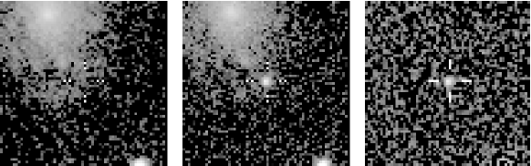
Figure 1: Discovery images for LSQ12gdj. Left: REF (galaxy template) image showing the host galaxy before the SN. Center: NEW image showing host galaxy + SN. Right: Subtraction SUB = NEW - REF, showing the SN alone. The thumbnails are $56^{\prime\prime}\times 56^{\prime\prime}$ square.

The Nearby Supernova Factory (SNfactory) reported that a spectrum taken 2013 Nov 10.2 UT with the SuperNova Integral Field Spectrograph (SNIFS; Lantz et al., 2004) on the University of Hawaii 2.2-m telescope was a good match to a 1991T-like SN Ia before maximum light as classified using SNID (Blondin & Tonry, 2007), and flagged it as a candidate super-Chandrasekhar-mass SN Ia (Cellier-Holzem et al., 2012). This classification was later confirmed by the first PESSTO spectrum in the time series described below, taken 2012 Nov 13 UT.

2.2 Photometry

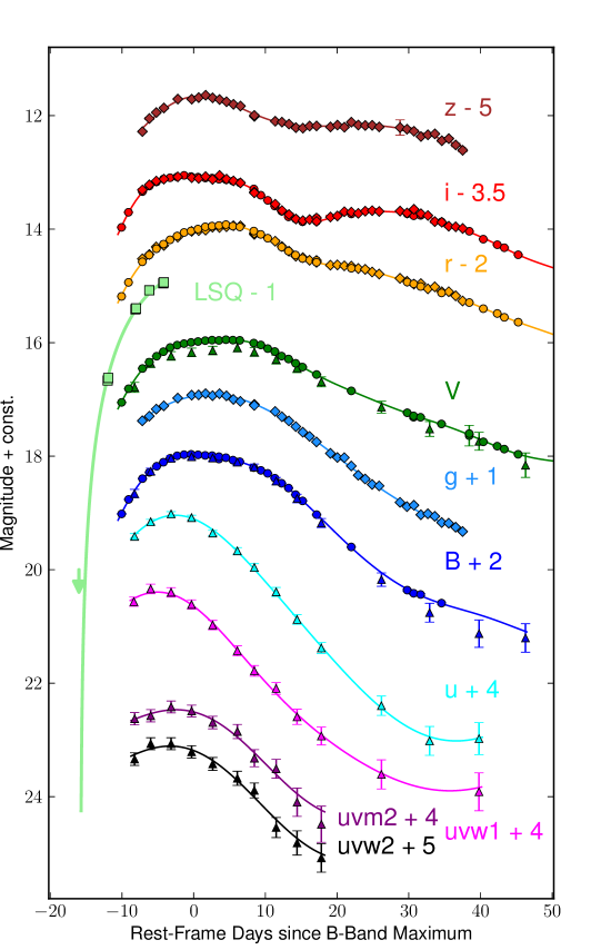
Figure 2: Multi-band light curves of LSQ12gdj. CSP and LCOGT points are shown as circles, Swift points are upward-facing triangles, and LSQ points are squares. Solid curves: Gaussian process regression fit to the data (see Rasmussen & Williams, 2006; Scalzo et al., 2014), except LSQ, for which the Arnett (1982) functional form is used (well-approximated by a $t^{2}$ rise at early times). Light curve phase is with respect to $B$-band maximum at MJD 56252.5 (2012 Nov 21.5).

Swift UVOT observations were triggered immediately after spectroscopic confirmation, providing comprehensive photometric coverage at UV wavelengths starting 8 days before $B$-band maximum light. The observations were reduced using aperture photometry according to the procedure in Brown et al. (2009), using the updated zeropoints, sensitivity corrections, and transmission curves of Breeveld et al. (2011).

Ground-based follow-up photometry was taken by the Carnegie Supernova Project II (CSP) using the Swope 1-m telescope at Las Campanas observatory, in the natural system CSP $BVr^{\prime}i^{\prime}$ filters, starting at 10 days before $B$-band maximum light. The SITe3 CCD detector mounted on the Swope has a 2048 $\times$ 4096 pix active area, with a pixel scale of 0.435 arcsec/pix; to reduce readout time, a 1200 $\times$ 1200 pix subraster is read out, for a field of view of $8.7\times 8.7$ arcmin. The images were reduced with standard CSP software including bias subtraction, linearity correction, flat fielding and exposure correction. A local sequence of 20 stars around the SN, covering a wide range of magnitudes, has been calibrated on more than 15 photometric nights into the natural system of the Swope telescope, using the reduction procedures described in Contreras et al. (2010) and the bandpass calibration procedures and transmission functions in Stritzinger et al. (2012). Template images for galaxy subtractions were taken with the Du Pont 2.5-m telescope under favorable seeing conditions on the nights of 2013 Oct 10–11, using the same filter set as the science images. PSF-fitting photometry was performed on the SN detections in the template-subtracted images, relative to the local sequence stars, measured with the standard IRAF (Tody, 1993) package daophot (Stetson, 1987).

Additional ground-based photometry was taken by the Las Cumbres Observatory Global Telescope Network (LCOGT). The LCOGT data were reduced using a custom pipeline developed by the LCOGT SN team, using standard procedures (pyraf, daophot, SWarp) in a python framework. PSF-fitting photometry is performed after subtraction of the background, estimated via a low-order polynomial fit.

The Swift UV photometry and the CSP/LCOGT optical photometry are shown in Tables LABEL:tbl:photometry-swift and LABEL:tbl:photometry-opt, respectively, and plotted in Figure 2. All ground-based magnitudes have been $S$-corrected to the appropriate standard system Landolt (1992); Fukugita et al. (2010). The natural-system CSP/LCOGT photometry is shown in Table LABEL:tbl:natphot (online-only).

Table 1: Ground-based photometry of LSQ12gdj in instrumental fluxes

MJD	Phasea	Flux (ADU)	Inst. Magb
56238.074	$-14.0$	$1610.9\pm 38.2$	$18.98\pm 0.03$
56238.158	$-13.9$	$1751.2\pm 44.2$	$18.89\pm 0.03$
56240.061	$-12.1$	$5407.8\pm 68.8$	$17.67\pm 0.01$
56240.144	$-12.0$	$5637.9\pm 77.6$	$17.62\pm 0.01$
56244.054	$-8.2$	$17167.6\pm 101.1$	$16.41\pm 0.01$
56244.138	$-8.1$	$17428.5\pm 108.0$	$16.40\pm 0.01$
56246.049	$-6.3$	$23382.5\pm 186.7$	$16.08\pm 0.01$
56248.044	$-4.3$	$26198.3\pm 230.2$	$15.95\pm 0.01$
56248.128	$-4.2$	$26575.1\pm 236.4$	$15.94\pm 0.01$

Table 2: Swift photometry of LSQ12gdj

MJD	Phasea	$uvw2$	$uvm2$	$uvw1$	$u$	$b$	$v$
56243.9	$-8.4$	$18.34\pm 0.11$	$18.63\pm 0.11$	$16.56\pm 0.08$	$15.41\pm 0.05$	$16.65\pm 0.07$	$16.77\pm 0.09$
56246.2	$-6.1$	$18.07\pm 0.10$	$18.57\pm 0.11$	$16.34\pm 0.08$	$15.16\pm 0.04$	$16.25\pm 0.06$	$16.34\pm 0.08$
56249.2	$-3.2$	$18.07\pm 0.10$	$18.42\pm 0.10$	$16.40\pm 0.08$	$15.02\pm 0.04$	$16.02\pm 0.05$	$16.21\pm 0.08$
56252.1	$-0.4$	$18.21\pm 0.11$	$18.49\pm 0.10$	$16.61\pm 0.08$	$15.08\pm 0.04$	$15.98\pm 0.05$	$16.15\pm 0.07$
56255.2	$2.6$	$18.42\pm 0.11$	$18.69\pm 0.11$	$16.98\pm 0.08$	$15.36\pm 0.05$	$16.00\pm 0.05$	$16.12\pm 0.07$
56258.7	$6.0$	$18.68\pm 0.12$	$18.85\pm 0.12$	$17.43\pm 0.09$	$15.67\pm 0.06$	$16.08\pm 0.05$	$16.07\pm 0.07$
56261.1	$8.4$	$18.89\pm 0.13$	$19.32\pm 0.15$	$17.78\pm 0.09$	$15.96\pm 0.07$	$16.17\pm 0.05$	$16.14\pm 0.07$
56264.3	$11.4$	$19.54\pm 0.18$	$19.51\pm 0.17$	$18.09\pm 0.10$	$16.39\pm 0.08$	$16.42\pm 0.06$	$16.27\pm 0.08$
56267.3	$14.3$	$19.82\pm 0.21$	$20.10\pm 0.25$	$18.59\pm 0.13$	$16.88\pm 0.09$	$16.73\pm 0.08$	$16.42\pm 0.08$
56270.8	$17.7$	$20.08\pm 0.25$	$20.48\pm 0.32$	$18.93\pm 0.16$	$17.38\pm 0.10$	$17.18\pm 0.08$	$16.66\pm 0.09$
56279.4	$26.1$	…	…	$19.61\pm 0.26$	$18.40\pm 0.17$	$18.18\pm 0.12$	$17.11\pm 0.10$
56286.3	$32.8$	…	…	…	$19.02\pm 0.25$	$18.76\pm 0.17$	$17.49\pm 0.13$
56293.4	$39.7$	…	…	$19.91\pm 0.33$	$18.98\pm 0.28$	$19.11\pm 0.24$	$17.71\pm 0.16$
56300.1	$46.2$	…	…	…	…	$19.17\pm 0.25$	$18.13\pm 0.22$

Table 3: Ground-based photometry of LSQ12gdj in the Landolt and SDSS standard systems

MJD	Phasea	$B$	$V$	$g$	$r$	$i$	$z$	Source
56242.1	$-10.2$	$17.02\pm 0.01$	$17.05\pm 0.01$	…	$17.19\pm 0.01$	$17.47\pm 0.01$	…	SWOPE
56243.1	$-9.2$	$16.76\pm 0.01$	$16.81\pm 0.01$	…	$16.94\pm 0.01$	$17.20\pm 0.01$	…	SWOPE
56245.0	$-7.3$	…	…	$16.38\pm 0.01$	$16.52\pm 0.01$	$16.81\pm 0.02$	$17.28\pm 0.01$	LCOGT
56245.1	$-7.2$	$16.40\pm 0.01$	$16.46\pm 0.01$	…	$16.57\pm 0.01$	$16.84\pm 0.01$	…	SWOPE
56246.0	$-6.3$	$16.29\pm 0.01$	$16.34\pm 0.01$	…	$16.46\pm 0.01$	$16.74\pm 0.01$	…	SWOPE
56246.0	$-6.3$	…	…	$16.30\pm 0.01$	$16.45\pm 0.02$	$16.72\pm 0.01$	$17.05\pm 0.02$	LCOGT
56247.0	$-5.3$	…	…	$16.17\pm 0.01$	$16.31\pm 0.02$	$16.65\pm 0.01$	$16.95\pm 0.02$	LCOGT
56247.1	$-5.3$	$16.18\pm 0.01$	$16.24\pm 0.01$	…	$16.35\pm 0.01$	$16.67\pm 0.01$	…	SWOPE
56248.1	$-4.3$	$16.11\pm 0.01$	$16.16\pm 0.01$	…	$16.26\pm 0.00$	$16.62\pm 0.01$	…	SWOPE
56248.1	$-4.3$	…	…	$16.11\pm 0.01$	$16.29\pm 0.01$	$16.62\pm 0.02$	$16.86\pm 0.02$	LCOGT
56249.0	$-3.4$	$16.04\pm 0.01$	$16.09\pm 0.01$	…	$16.19\pm 0.00$	$16.59\pm 0.01$	…	SWOPE
56250.0	$-2.4$	$15.99\pm 0.01$	$16.04\pm 0.01$	…	$16.12\pm 0.01$	$16.58\pm 0.01$	…	SWOPE
56250.1	$-2.3$	…	…	$15.98\pm 0.01$	$16.14\pm 0.02$	$16.58\pm 0.01$	$16.71\pm 0.02$	LCOGT
56251.0	$-1.4$	$15.97\pm 0.01$	$16.02\pm 0.01$	…	$16.06\pm 0.01$	$16.55\pm 0.01$	…	SWOPE
56252.0	$-0.5$	$15.97\pm 0.01$	$16.00\pm 0.01$	…	$16.03\pm 0.01$	$16.57\pm 0.01$	…	SWOPE
56252.1	$-0.4$	…	…	$15.93\pm 0.01$	$16.04\pm 0.01$	$16.59\pm 0.01$	$16.71\pm 0.01$	LCOGT
56253.0	$0.5$	$15.98\pm 0.01$	$15.98\pm 0.01$	…	$16.00\pm 0.00$	$16.58\pm 0.01$	…	SWOPE
56253.1	$0.6$	…	…	$15.92\pm 0.01$	$16.03\pm 0.01$	$16.61\pm 0.01$	$16.68\pm 0.01$	LCOGT
56254.1	$1.5$	$15.99\pm 0.01$	$15.96\pm 0.01$	…	$15.96\pm 0.01$	$16.60\pm 0.01$	…	SWOPE
56254.1	$1.6$	…	…	$15.90\pm 0.01$	$16.02\pm 0.01$	$16.58\pm 0.02$	$16.64\pm 0.01$	LCOGT
56255.1	$2.5$	$15.99\pm 0.01$	$15.96\pm 0.01$	…	$15.95\pm 0.01$	$16.60\pm 0.01$	…	SWOPE
56255.1	$2.5$	…	…	$15.93\pm 0.01$	$15.97\pm 0.01$	$16.62\pm 0.01$	$16.69\pm 0.02$	LCOGT
56256.1	$3.4$	$16.05\pm 0.02$	$15.96\pm 0.01$	…	$15.94\pm 0.01$	$16.62\pm 0.01$	…	SWOPE
56256.1	$3.5$	…	…	$15.90\pm 0.01$	$15.97\pm 0.01$	$16.55\pm 0.02$	$16.72\pm 0.02$	LCOGT
56257.1	$4.4$	$16.03\pm 0.01$	$15.95\pm 0.01$	…	$15.92\pm 0.01$	$16.63\pm 0.01$	…	SWOPE
56257.1	$4.5$	…	…	$15.94\pm 0.01$	$15.96\pm 0.01$	$16.62\pm 0.02$	$16.76\pm 0.02$	LCOGT
56258.1	$5.4$	$16.07\pm 0.01$	$15.95\pm 0.01$	…	$15.95\pm 0.01$	$16.65\pm 0.01$	…	SWOPE
56258.1	$5.5$	…	…	$16.00\pm 0.01$	$15.94\pm 0.01$	$16.65\pm 0.01$	$16.80\pm 0.02$	LCOGT
56259.0	$6.3$	$16.10\pm 0.01$	$15.96\pm 0.01$	…	$15.96\pm 0.01$	$16.68\pm 0.01$	…	SWOPE
56259.1	$6.4$	…	…	$16.03\pm 0.01$	$15.94\pm 0.01$	$16.69\pm 0.03$	$16.83\pm 0.02$	LCOGT
56261.1	$8.3$	$16.20\pm 0.01$	$16.01\pm 0.01$	…	$16.03\pm 0.01$	$16.79\pm 0.01$	…	SWOPE
56261.1	$8.4$	…	…	$16.09\pm 0.01$	$16.09\pm 0.01$	$16.85\pm 0.01$	$17.01\pm 0.01$	LCOGT
56262.1	$9.3$	$16.25\pm 0.01$	$16.04\pm 0.01$	…	$16.09\pm 0.01$	$16.90\pm 0.01$	…	SWOPE
56263.1	$10.2$	$16.30\pm 0.01$	$16.10\pm 0.01$	…	$16.16\pm 0.01$	$16.99\pm 0.01$	…	SWOPE
56264.1	$11.2$	$16.39\pm 0.01$	$16.16\pm 0.01$	…	…	$17.09\pm 0.01$	…	SWOPE
56264.1	$11.3$	…	…	$16.21\pm 0.01$	$16.21\pm 0.03$	$17.06\pm 0.00$	$17.10\pm 0.02$	LCOGT

Table 3: Ground-based photometry of LSQ12gdj, cont’d.

MJD	Phasea	$B$	$V$	$g$	$r$	$i$	$z$	Source
56265.1	$12.2$	$16.48\pm 0.01$	$16.24\pm 0.01$	…	$16.31\pm 0.01$	$17.18\pm 0.01$	…	SWOPE
56265.1	$12.2$	…	…	$16.31\pm 0.01$	$16.31\pm 0.01$	$17.17\pm 0.01$	$17.11\pm 0.01$	LCOGT
56266.1	$13.1$	$16.56\pm 0.01$	$16.29\pm 0.01$	…	$16.39\pm 0.01$	$17.28\pm 0.01$	…	SWOPE
56266.1	$13.2$	…	…	$16.38\pm 0.01$	$16.39\pm 0.01$	$17.24\pm 0.03$	$17.15\pm 0.02$	LCOGT
56267.1	$14.1$	$16.68\pm 0.01$	$16.36\pm 0.01$	…	$16.46\pm 0.01$	$17.32\pm 0.01$	…	SWOPE
56267.1	$14.2$	…	…	$16.48\pm 0.01$	$16.48\pm 0.01$	$17.32\pm 0.01$	$17.21\pm 0.02$	LCOGT
56268.1	$15.1$	$16.79\pm 0.01$	$16.43\pm 0.01$	…	$16.52\pm 0.01$	$17.37\pm 0.01$	…	SWOPE
56268.1	$15.1$	…	…	$16.58\pm 0.01$	$16.50\pm 0.01$	$17.35\pm 0.01$	$17.22\pm 0.02$	LCOGT
56269.1	$16.1$	…	…	$16.65\pm 0.01$	$16.55\pm 0.01$	$17.33\pm 0.01$	$17.18\pm 0.02$	LCOGT
56270.1	$17.0$	…	…	$16.75\pm 0.01$	$16.55\pm 0.01$	$17.30\pm 0.02$	$17.18\pm 0.02$	LCOGT
56270.1	$17.0$	$17.03\pm 0.01$	$16.56\pm 0.01$	…	$16.58\pm 0.01$	$17.36\pm 0.01$	…	SWOPE
56272.1	$19.0$	…	…	$16.95\pm 0.01$	$16.63\pm 0.02$	$17.29\pm 0.03$	$17.20\pm 0.02$	LCOGT
56273.1	$20.0$	…	…	$17.02\pm 0.01$	$16.63\pm 0.01$	$17.27\pm 0.01$	$17.17\pm 0.01$	LCOGT
56274.1	$20.9$	…	…	$17.03\pm 0.01$	$16.65\pm 0.01$	$17.19\pm 0.01$	$17.20\pm 0.02$	LCOGT
56275.1	$21.9$	$17.60\pm 0.01$	$16.85\pm 0.01$	…	$16.69\pm 0.01$	$17.23\pm 0.01$	…	SWOPE
56275.1	$21.9$	…	…	$17.17\pm 0.01$	$16.65\pm 0.02$	$17.20\pm 0.01$	$17.12\pm 0.01$	LCOGT
56276.1	$22.9$	…	…	$17.34\pm 0.01$	$16.69\pm 0.01$	$17.22\pm 0.01$	$17.17\pm 0.01$	LCOGT
56277.1	$23.8$	…	…	$17.40\pm 0.01$	$16.71\pm 0.03$	$17.18\pm 0.01$	$17.17\pm 0.02$	LCOGT
56278.1	$24.8$	…	…	$17.50\pm 0.01$	$16.76\pm 0.01$	$17.17\pm 0.03$	$17.17\pm 0.01$	LCOGT
56279.1	$25.8$	…	…	$17.52\pm 0.01$	$16.79\pm 0.01$	$17.19\pm 0.01$	$17.20\pm 0.02$	LCOGT
56282.1	$28.7$	…	…	$17.81\pm 0.01$	$16.87\pm 0.02$	$17.18\pm 0.01$	$17.21\pm 0.14$	LCOGT
56283.1	$29.7$	…	…	$17.89\pm 0.01$	$16.92\pm 0.01$	$17.22\pm 0.01$	$17.24\pm 0.03$	LCOGT
56283.1	$29.7$	$18.36\pm 0.02$	$17.24\pm 0.01$	…	$16.93\pm 0.01$	$17.23\pm 0.01$	…	SWOPE
56284.0	$30.6$	$18.42\pm 0.02$	$17.31\pm 0.02$	…	$16.96\pm 0.01$	$17.26\pm 0.01$	…	SWOPE
56284.1	$30.6$	…	…	$17.86\pm 0.02$	$16.97\pm 0.01$	$17.15\pm 0.01$	$17.28\pm 0.02$	LCOGT
56285.0	$31.6$	$18.44\pm 0.02$	$17.31\pm 0.01$	…	$17.01\pm 0.01$	$17.26\pm 0.01$	…	SWOPE
56285.1	$31.6$	…	…	$18.03\pm 0.01$	$16.96\pm 0.01$	$17.23\pm 0.01$	$17.37\pm 0.02$	LCOGT
56286.1	$32.6$	…	…	$18.02\pm 0.01$	$17.05\pm 0.01$	$17.26\pm 0.01$	$17.34\pm 0.02$	LCOGT
56287.1	$33.5$	…	…	$18.06\pm 0.01$	$17.02\pm 0.02$	$17.37\pm 0.02$	$17.32\pm 0.01$	LCOGT
56288.0	$34.5$	$18.59\pm 0.02$	$17.43\pm 0.01$	…	$17.12\pm 0.01$	$17.37\pm 0.01$	…	SWOPE
56288.1	$34.5$	…	…	$18.17\pm 0.01$	$17.10\pm 0.01$	$17.38\pm 0.01$	$17.44\pm 0.02$	LCOGT
56289.1	$35.5$	…	…	$18.18\pm 0.02$	$17.10\pm 0.02$	$17.45\pm 0.03$	$17.41\pm 0.02$	LCOGT
56290.1	$36.4$	…	…	$18.25\pm 0.02$	$17.18\pm 0.01$	$17.46\pm 0.01$	$17.52\pm 0.03$	LCOGT
56291.1	$37.4$	…	…	$18.33\pm 0.01$	$17.27\pm 0.01$	$17.49\pm 0.01$	$17.61\pm 0.02$	LCOGT
56292.0	$38.4$	…	$17.62\pm 0.02$	…	$17.29\pm 0.01$	$17.54\pm 0.01$	…	SWOPE
56294.0	$40.3$	…	$17.77\pm 0.02$	…	$17.40\pm 0.01$	$17.68\pm 0.01$	…	SWOPE
56296.1	$42.2$	…	$17.84\pm 0.02$	…	$17.49\pm 0.01$	$17.77\pm 0.01$	…	SWOPE
56297.1	$43.2$	…	$17.89\pm 0.02$	…	$17.55\pm 0.01$	$17.83\pm 0.01$	…	SWOPE
56299.1	$45.2$	…	$17.98\pm 0.02$	…	$17.64\pm 0.01$	$17.95\pm 0.01$	…	SWOPE
56316.0	$61.6$	…	$18.48\pm 0.04$	…	$18.31\pm 0.03$	$18.77\pm 0.04$	…	SWOPE
56318.0	$63.6$	…	$18.55\pm 0.03$	…	…	…	…	SWOPE

Table 4: Ground-based photometry of LSQ12gdj in the natural systems of the Swope and LCOGT telescopes

MJD	Phasea	$B$	$V$	$g$	$r$	$i$	$z$	Source
56242.1	$-10.2$	$17.02\pm 0.01$	$17.05\pm 0.01$	…	$17.20\pm 0.01$	$17.52\pm 0.01$	…	SWOPE
56243.1	$-9.2$	$16.76\pm 0.01$	$16.81\pm 0.01$	…	$16.95\pm 0.01$	$17.25\pm 0.01$	…	SWOPE
56245.0	$-7.3$	…	…	$16.39\pm 0.01$	$16.53\pm 0.01$	$16.83\pm 0.02$	$17.25\pm 0.01$	LCOGT
56245.1	$-7.2$	$16.39\pm 0.01$	$16.46\pm 0.01$	…	$16.60\pm 0.01$	$16.88\pm 0.01$	…	SWOPE
56246.0	$-6.3$	$16.28\pm 0.01$	$16.35\pm 0.01$	…	$16.48\pm 0.01$	$16.78\pm 0.01$	…	SWOPE
56246.0	$-6.3$	…	…	$16.31\pm 0.01$	$16.46\pm 0.02$	$16.74\pm 0.01$	$17.02\pm 0.02$	LCOGT
56247.0	$-5.3$	…	…	$16.18\pm 0.01$	$16.32\pm 0.02$	$16.67\pm 0.01$	$16.91\pm 0.02$	LCOGT
56247.1	$-5.3$	$16.17\pm 0.01$	$16.24\pm 0.01$	…	$16.37\pm 0.01$	$16.71\pm 0.01$	…	SWOPE

2.3 Spectroscopy

A full spectroscopic time series was taken by the Public ESO Spectroscopic Survey for Transient Objects (PESSTO), using the EFOSC2 spectrograph on the ESO New Technology Telescope (NTT) at La Silla Observatory, comprising seven spectra taken between 2012 Nov 13 and 2013 Jan 13 UT. The $gr11$ and $gr16$ gratings were used, covering the entire wavelength range 3360–10330 Å at 13 Å resolution. The spectra were reduced using the pyraf package as part of a custom-built, Python-based pipeline written for PESSTO; the pipeline includes corrections for bias and fringing, wavelength and flux calibration, correction for telluric absorption and a cross-check of the wavelength calibration using atmospheric emission lines.

Three spectra of LSQ12gdj were obtained around maximum light by CSP using the Las Campanas 2.5-m du Pont telescope and WFCCD. The spectral resolution is 8 Å, as measured from the FWHM of the HeNeAr comparison lines. A complete description of data reduction procedures can be found in Hamuy et al. (2006).

An additional five optical spectra were taken with the WiFeS integral field spectrograph on the ANU 2.3-m telescope at Siding Spring Observatory. WiFeS spectra were obtained using the B3000 and R3000 gratings, providing wavelength coverage in the range 3500–9600 Å with a FWHM resolution for the point-spread function (PSF) of 1.5 Å (blue channel) and 2.5 Å (red channel). Data cubes for WiFeS observations were produced using the PyWiFeS software (Childress et al., 2013b). Spectra of the SN were extracted from final data cubes using a PSF-weighted extraction technique with a simple symmetric Gaussian PSF, and the width of this Gaussian was measured directly from the data cube. Background subtraction was performed by calculating the median background spectrum across all pixels outside a distance from the SN equal to about three times the seeing disk (typically $1^{\prime\prime}.5$–$2^{\prime\prime}$ FWHM). This technique produced good results for the WiFeS spectra of LSQ12gdj, due to the negligible galaxy background and good spatial flatfielding from the PyWiFeS pipeline.

The observation log for all spectra presented is shown in Table LABEL:tbl:spectroscopy, and the spectra are plotted in Figure 3. All spectra will be publicly available through WISeREP (Yaron & Gal-Yam, 2012).

Table 5: Optical spectroscopy of LSQ12gdj

UT	MJD	Phasea	Telescope	Exposure	Wavelength	Observersb
Date		(days)	/ Instrument	Time (s)	Range (Å)
2012 Nov 13.13	56244.1	$-8.1$	NTT-3.6m / EFOSC	1500	3360–10000	PESSTO
2012 Nov 15.14	56246.1	$-6.2$	NTT-3.6m / EFOSC	1500	3360–10000	PESSTO
2012 Nov 17.43	56248.4	$-4.0$	ANU-2.3m / WiFeS	1200	3500–9550	NS
2012 Nov 19.52	56250.5	$-1.9$	ANU-2.3m / WiFeS	1200	3500–9550	MC
2012 Nov 19.92	56250.9	$-1.6$	DuPont / WFCCD	$2\times 600$	3580–9620	NM
2012 Nov 20.43	56251.4	$-1.1$	ANU-2.3m / WiFeS	1200	3500–9550	MC
2012 Nov 20.93	56251.9	$-0.6$	DuPont / WFCCD	$2\times 600$	3580–9620	NM
2012 Nov 21.45	56252.5	$-0.1$	ANU-2.3m / WiFeS	1200	3500–9550	MC
2012 Nov 21.85	56252.9	$+0.3$	DuPont / WFCCD	$2\times 600$	3580–9620	NM
2012 Nov 23.15	56254.1	$+1.6$	NTT-3.6m / EFOSC	900	3360–10000	PESSTO
2012 Nov 29.47	56260.5	$+7.7$	ANU-2.3m / WiFeS	1200	3500–9550	CL,BS
2012 Dec 06.12	56267.1	$+14.2$	NTT-3.6m / EFOSC	1500	3360–10000	PESSTO
2012 Dec 14.13	56275.1	$+21.9$	NTT-3.6m / EFOSC	1500	3360–10000	PESSTO
2012 Dec 23.13	56284.1	$+30.7$	NTT-3.6m / EFOSC	900	3360–10000	PESSTO
2013 Jan 13.05	56305.1	$+51.0$	NTT-3.6m / EFOSC	$2\times 1500$	3360–10000	PESSTO

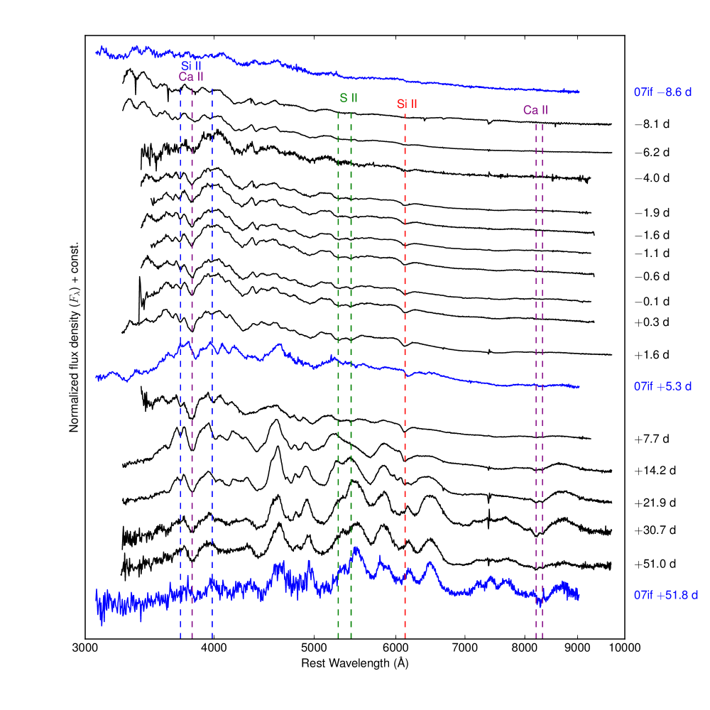
Figure 3: Spectral time series of LSQ12gdj (black solid lines, phase labels on right), shown with spectra of SN 2007if (blue solid lines, rest-frame phase labels on right; Scalzo et al., 2012) for comparison. All spectra have been rebinned to 5 Å. Constant velocity locations for absorption minima of various intermediate-mass element absorption features are marked with dashed lines: purple, Ca 2 H+K and NIR (10000 $\mathrm{km~{}s}^{-1}$); blue, Si 2 $\lambda\lambda 3858,4129$ (11500 $\mathrm{km~{}s}^{-1}$); red, Si 2 $\lambda\lambda 6355$ (11000 $\mathrm{km~{}s}^{-1}$); green, S 2 $\lambda\lambda 5454,5640$ (10500 $\mathrm{km~{}s}^{-1}$).

3 Analysis

In this section we discuss quantities derived from the photometry and spectroscopy in more detail. We characterize the spectroscopic evolution of LSQ12gdj, including the velocities of common absorption features, in §3.1. We discuss the broad-band light curves of LSQ12gdj and estimate the host galaxy extinction in §3.2. Finally, we describe the construction of a bolometric light curve for LSQ12gdj in §3.3, including correction for unobserved NIR flux and the process of solving for a low-resolution broad-band spectral energy distribution (SED).

3.1 Spectral Features and Velocity Evolution

Figure 3 shows the spectroscopic evolution of LSQ12gdj, with spectra of the super-Chandrasekhar-mass SN 2007if included for comparison. The early spectra show evidence for a hot photosphere, with a blue continuum and absorption features dominated by Fe 2 and Fe 3, typical of 1991T-like SNe Ia Filippenko et al. (1992); Phillips et al. (1992). These include absorption complexes near 3500 Å, attributed to iron-peak elements (Ni 2, Co 2, and Cr 2) in SN 2007if (Scalzo et al., 2010). The prominence of hot iron-peak elements in the outer layers is consistent with a great deal of ${}^{56}\mathrm{Ni}$ being produced, and/or with significant mixing of ${}^{56}\mathrm{Ni}$ throughout the outer layers of ejecta during the explosion. Si 2 $\lambda 5972$ is not visible. Si 2 $\lambda 6355$ and Ca 2 H+K are weak throughout the evolution.

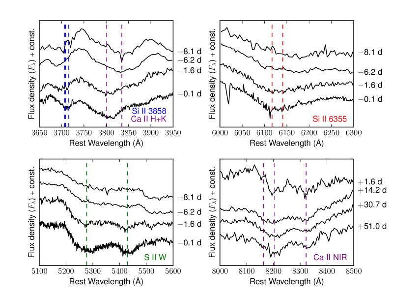
Figure 4: Subranges of spectra showing absorption line profiles of intermediate-mass elements in the LSQ12gdj spectral time series. Vertical dashed lines indicate the velocity of every component of each absorbing multiplet near maximum light. Phases shown along the right-hand edges of the plots are in rest-frame days with respect to $B$-band maximum light, as in Figure 3.

Figure 4 shows subranges of the spectra highlighting common intermediate-mass element lines at key points in their evolution. LSQ12gdj shows unusually narrow intermediate-mass-element signatures. The Ca 2 H+K absorption is narrow enough ($\sim 6000$ $\mathrm{km~{}s}^{-1}$FWHM) that the minimum is unblended with neighboring Si 2 $\lambda 3858$; an inflection in the line profile redwards of the main minimum could be signs that the doublet structure is just barely unresolved. At later phases, the two reddest components of the Ca 2 NIR triplet show distinct minima near 12000 $\mathrm{km~{}s}^{-1}$. The Si 2 $\lambda 6355$ line profile near maximum light has a flat, boxy minimum. Spectra at the earliest phases show absorption minima near the expected positions of all of these lines near maximum light, but with unexpected shapes; these lines may not correspond physically to the nearest familiar feature in each case, but if they do, they may yield interesting information about the level populations to detailed modelling which properly accounts for the ionization balance. An example of such ambiguity is the feature near 3650 Å in the pre-maximum spectra, the position of which is consistent with high-velocity Ca 2 as in normal SNe Ia, but is also near the expected position of Si 3 around 12000 $\mathrm{km~{}s}^{-1}$.

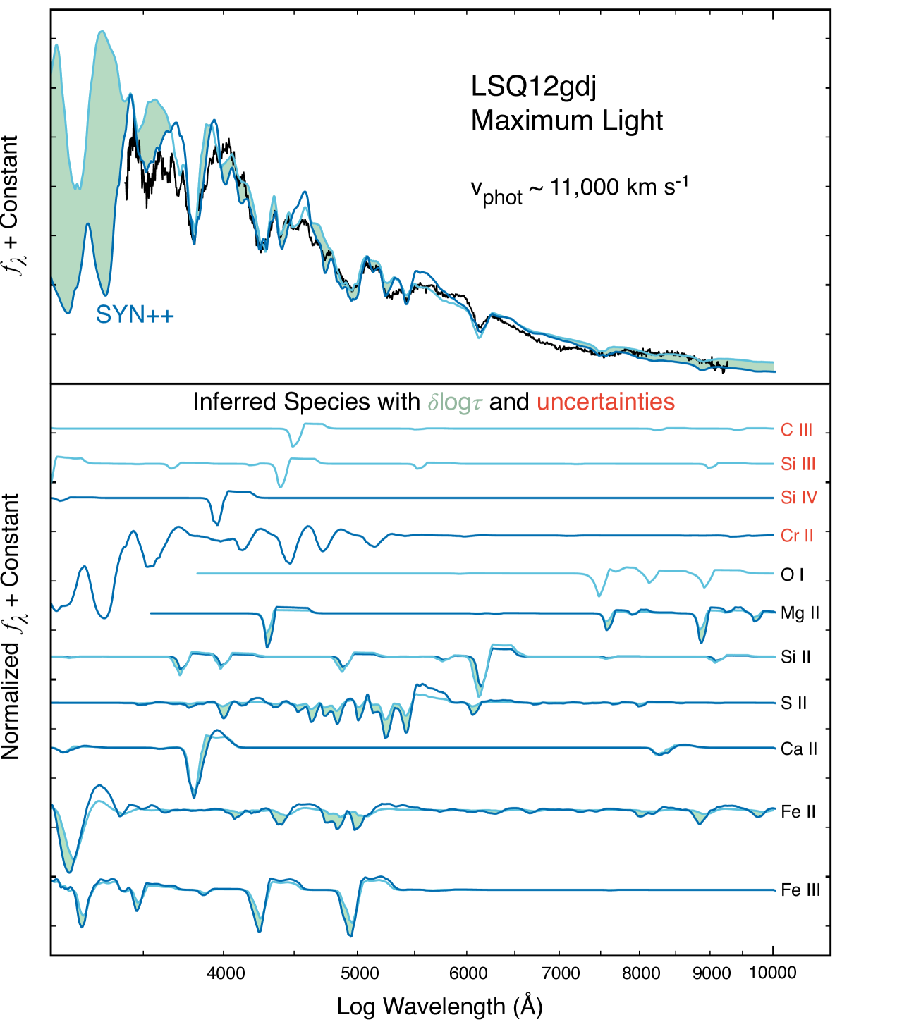
Figure 5: Maximum light SYN++ fit comparisons between two best fits, with and without the inclusion of Cr 2. Species listed in red denote degenerate solutions for some observed absorption features, while subsequent uncertainties associated with respective line strengths ($\log\,\tau$) between our two best fits are represented as a band of aquamarine.

To identify various line features in a more comprehensive manner, we fit the maximum-light spectrum of LSQ12gdj using SYN++ (Thomas et al., 2011), shown in Figure 5. While LSQ12gdj displays many features typical of SNe Ia near maximum light, our fit also suggests contributions from higher ionization species, e.g., C 3 $\lambda$4649 over Fe 2/S 2 absorption complexes, or Si 3 near 3650 Å and 4400 Å in the pre-maximum spectra. These identifications, though tentative (labelled in red in Figure 5), are consistent with spectroscopic behaviors seen in shallow-silicon events prior to maximum light (Branch et al., 2006). The suggestion of C 3 $\lambda 4649$ near 18,000 $\mathrm{km~{}s}^{-1}$ is tantalizing, but ambiguous, and no corresponding C 2 $\lambda 6580$ absorption is evident. Cr 2 is an intriguing possibility, since it provides a better fit in the bluest part of the spectrum and simultaneously contributes strong line blanketing in the unobserved UV part of the spectrum; such line blanketing is in line with the sharp cutoff of our photometry-based SED in the Swift bands (see §3.3). However, given the degeneracies involved in identifying highly blended species, we do not consider Cr 2 to have been definitively detected in LSQ12gdj.

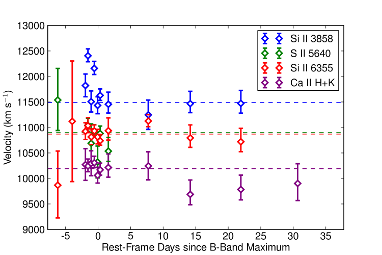
Figure 6: Blueshift velocities of absorption minima of intermediate-mass element lines in the LSQ12gdj spectral time series. Horizontal dashed lines indicate the median velocity. Asymmetric error bars represent the 68% CL region for the absorption line minimum.

We measure the absorption minimum velocities of common lines in a less model-dependent way using a method similar to Scalzo et al. (2012). We resample each spectrum to $\log(\lambda)$, i.e., to velocity space, then smooth it with wide (“continuum”; $\sim 75000$ $\mathrm{km~{}s}^{-1}$) and narrow (“lines”; $\sim 3500$ $\mathrm{km~{}s}^{-1}$) third-order Savitzsky-Golay filters, which retain detail in the intrinsic line shapes more effectively than rebinning or conventional Gaussian filtering. After dividing out the continuum to produce a smoothed spectrum with only line features, we measure the absorption minima and estimate the statistical errors by Monte Carlo sampling. We track the full covariance matrix of the spectrum from the original reduced data to the final smoothed version, and use its Cholesky decomposition to produce Monte Carlo realizations. We add in quadrature a systematic error equal to the RMS spectrograph resolution, which may affect the observed line minimum since we are not assuming a functional form (e.g. a Gaussian) for the line profile. The resulting velocities are shown in Figure 6. In calculating velocities from wavelengths, we assume nearby component multiplets are blended, with the rest wavelength of each line being the $g$-weighted rest wavelengths of the multiplet components, although this approximation may break down for some lines (see Figure 4).

LSQ12gdj shows slow velocity evolution in the absorption minima of intermediate mass elements, again characteristic of SN 1991T (Phillips et al., 1992) and other candidate super-Chandrasekhar-mass events with 1991T-like spectra (Scalzo et al., 2010, 2012). At early times, familiar absorption features of intermediate-mass elements are either ambiguously identified or too weak for their properties to be measured reliably, but come clearly into focus by maximum light. Before maximum, the measured velocities for Si 2 $\lambda 3858$ differ by as much as 1000 $\mathrm{km~{}s}^{-1}$ between neighboring WiFeS and CSP spectra. The most likely source of the discrepancy is systematic error in the continuum estimation for this shallow line near the blue edge of each spectrograph’s sensitivity, since the relative prominence of the local maxima on either side of the line differ between CSP and WiFeS. For other line minima, measurements from CSP and from WiFeS are consistent with each other within the errors. For both Si 2 $\lambda 3858$ and Si 2 $\lambda 6355$, $\dot{v}_{\mathrm{Si}}<10$ $\mathrm{km~{}s}^{-1}$ from maximum light until those lines become fully blended with developing Fe 2 lines more than three weeks past $B$-band maximum. The Si 2 plateau velocity is higher ($\sim 11000$ $\mathrm{km~{}s}^{-1}$) than any of the Scalzo et al. (2012) SNe. The velocity of Ca 2 H+K seems to decrease by about 500 $\mathrm{km~{}s}^{-1}$ between day $+7$ and day $+14$, but on the whole it remains steady near 10000 $\mathrm{km~{}s}^{-1}$, with a velocity gradient consistent with that of Si 2. The S 2 $\lambda\lambda 5454,5640$ “W” feature, which often appears at lower velocities than Si 2, also appears around 11000 $\mathrm{km~{}s}^{-1}$ until blending with developing Fe 2 features erases it.

Such velocity plateaus are predicted by models with density enhancements in the outer ejecta, resulting from interaction with overlying material at early times (Quimby et al., 2007). These models include the DET2ENV2, DET2ENV4, and DET2ENV6 “tamped detonations” of Höflich & Khohklov (1996), hereafter collectively called “DET2ENVN”, and the “pulsating delayed detonations” by the same authors. In a tamped detonation, the ejecta interact with an external envelope; in a pulsating delayed detonation, an initial pulsation fails to unbind the white dwarf, and a shock is formed when the outer layers fall back onto the inner layers before the final explosion. The asymmetric models of Maeda et al. (2010b, 2011) also produce low velocity gradients, although in this case the density enhancement occurs only along the line of sight.

Alternatively, the plateau may trace not the density but the composition of the ejecta, i.e., may simply mark the outer edge of the iron-peak element core of the ejecta. The relatively normal SN Ia 2012fr (Childress et al., 2013a), for example, also featured extremely narrow (FWHM $<3000$ $\mathrm{km~{}s}^{-1}$) absorption features. SN 2012fr showed prominent high-velocity Si 2 absorption features, making it incompatible with a tamped detonation explosion scenario, since any SN ejecta above the shock velocity would have been swept into the reverse-shock shell. No signs of high-velocity absorption features from Ca, Si, or S are clearly evident in LSQ12gdj, although we might expect such material to be difficult to detect in shallow-silicon events like LSQ12gdj (Branch et al., 2006).

3.2 Maximum-Light Behavior, Colors, and Extinction

The reddening due to Galactic dust extinction towards the host of LSQ12gdj is $E(B-V)_{\mathrm{MW}}=0.021$ mag (Schlafly & Finkbeiner , 2011). LSQ12gdj was discovered on the outskirts of a spiral galaxy viewed face-on, so we expect minimal extinction by dust in the host galaxy. The equivalent width of Na 1 D absorption is $0.05\pm 0.03$ Å Maguire et al. (2013), also consistent with little to no host galaxy extinction. A fit to the Folatelli et al. (2010) version of the Lira relation (Phillips et al., 1999) to the CSP $B$ and $V$ light curves suggests $E(B-V)_{\mathrm{host}}=0.02\pm 0.08$ mag, consistent with zero.

To obtain more precise quantitative constraints for use in later modeling, we apply a multi-band light curve Bayesian analysis method to the CSP light curve of LSQ12gdj, trained on normal SNe Ia with a range of decline rates (Burns et al., 2014). This method provides joint constraints on $E(B-V)_{\mathrm{host}}$ and the slope $R_{V,\mathrm{host}}$ of a Cardelli et al. (1988) dust law. We find $E(B-V)_{\mathrm{host}}=0.013\pm 0.005$ mag and $R_{V}=1.66\pm 1.66$ (a truncated Gaussian with $0<R_{V}<10$), with covariance $C(E(B-V)_{\mathrm{host}},R_{V,\mathrm{host}})=-0.0039$ mag. We adopt these values for our analysis.

As in Scalzo et al. (2014), we perform Gaussian process (GP) regression on the light curve of each individual band, using the Python module sklearn (Pedregosa et al., 2011), as a convenient form of interpolation for missing data. Gaussian process regression is a machine learning technique which can be used to fit generic smooth curves to data without assuming a particular functional form; we refer the reader to Rasmussen & Williams (2006) for more details. Neighboring points on the GP fit are covariant; we use a squared-exponential covariance function $k(t,t^{\prime})=e^{-(t-t^{\prime})^{2}/2\tau^{2}}$, with $0.5<\tau<2.0$. When performing the fit, we include an extra term $\sigma_{i}^{2}\delta(t-t_{i})$ describing the statistical noise on the observations at times $t_{i}$ with errors $\sigma_{i}$; we neglect this noise term when predicting values from the fit.

Figure 2 shows the light curve of LSQ12gdj in all available bands, $S$-corrected to the appropriate standard system: LSQ; Swift UVOT $uvw1$, $uvm2$, $uvw2$, and $ubv$; Landolt $BV$; and SDSS $griz$. Using the CSP bands, the SiFTO light curve fitter (Conley et al., 2008) gives a light curve stretch $s=1.13\pm 0.01$ and MJD of $B$-band maximum $56253.4$. The SALT2.2 light curve fitter (Guy et al., 2007, 2010) gives consistent results ($x_{1}=0.96\pm 0.05$, $c=-0.048\pm 0.026$), though with a slightly later date for $B$-band maximum (MJD = 56253.8). Using one-dimensional GP regression fits to each separate band yields $B$-band maximum at MJD 56252.5 (2012 Nov 21.5, which we adopt henceforth), colour at $B$-band maximum $(B-V)_{\mathrm{max}}=-0.019\pm 0.005$, $\Delta m_{15}(B)=0.74\pm 0.01$, and peak magnitudes $m_{B}=15.972\pm 0.004$, $m_{V}=15.947\pm 0.004$. These errors are statisical only; systematic errors are probably around 2%. After correction for the mean expected reddening, we derive peak absolute magnitudes $M_{B}=-19.78$, $M_{V}=-19.77$, using a distance modulus $\mu=35.60\pm 0.07$ derived from the redshift assuming a $\Lambda$CDM cosmology with $H_{0}=67.3$ $\mathrm{km~{}s}^{-1}$ Mpc^-1 (Ade et al., 2013) and a random peculiar velocity of 300 $\mathrm{km~{}s}^{-1}$.

We find a fairly substantial ($\sim 0.2$ mag) mismatch between Swift $b$ and CSP $B$, and between Swift $v$ and CSP $V$, near maximum light; at later times, Swift and CSP observations agree within the errors (of the Swift points). The shape of the light curve is strongly constrained by CSP data, so we use CSP data in constructing the bolometric light curve at a given phase when both Swift and CSP observations are available.

The second maximum in the CSP $i$ light curve appears earlier ($+25$ days) than expected for LSQ12gdj’s $\Delta m_{15}(B)$ ($+30$ days Folatelli et al., 2010). The contrast of the second maximum is also fairly low, with a difference of $-0.63$ mag with the first maximum and $+0.20$ mag with the preceding minimum. Similar behavior is seen in LCOGT $z$. These properties are typical of low-${}^{56}\mathrm{Ni}$ explosions among the Chandrasekhar-mass models of Kasen (2006), difficult to reconcile with LSQ12gdj’s high luminosity. The low contrast persists even when CSP $i$ and LCOGT $z$ are $S$-corrected to Landolt $I$ for more direct comparison with Kasen (2006). If LSQ12gdj synthesized a high mass of ${}^{56}\mathrm{Ni}$, comparison with the models of Kasen (2006) suggests that LSQ12gdj has substantial mixing of ${}^{56}\mathrm{Ni}$ into its outer layers (as we might expect from its spectrum), a high yield of stable iron-peak elements, or both.

Fitting a $t^{2.0\pm 0.2}$ rise to LSQ points more than a week before $B$-band maximum light suggests an explosion date of MJD 56235.9, giving a $B$-band rise time of $16.2\pm 0.3$ days. The pre-explosion upper limits are compatible with a $t^{2}$ rise, but do not permit LSQ12gdj to be visible much before $B$-band phase $-16$. The $t^{2}$ functional form is at best approximate; depending on how ${}^{56}\mathrm{Ni}$ is distributed in the outer layers, the finite diffusion time of photons from ${}^{56}\mathrm{Ni}$ decay could result in a “dark phase” before the onset of normal emission (Hachinger et al., 2013; Piro & Nakar, 2013, 2014; Mazzali et al., 2014). Nevertheless, LSQ12gdj has a somewhat shorter visible rise than other SNe Ia with similar decline rates (Ganeshalingam et al., 2011), and much shorter than the 24-day visible rise of SN 2007if (Scalzo et al., 2010) determined by the same method.

3.3 Bolometric Light Curve

We construct a bolometric light curve for LSQ12gdj in the rest-frame wavelength range 1550–23100 Å using the available photometry, as follows.

We first generate quasi-simultaneous measurements of all bandpasses at each epoch in Tables LABEL:tbl:photometry-opt and LABEL:tbl:photometry-swift. We interpolate the values of missing measurements at each using the GP fits shown in Figure 2. After observations from a given band cease because the SN is no longer detected against the background, we estimate upper limits on the flux by assuming that the mean colours of the SN do not change since the last available observation — in particular that the SN does not become bluer in the Swift bands. If the last measurement in band $j$ was taken at time $t_{\mathrm{last},j}$, then at all future times $t_{i}$ we form the predictions

$$m_{i,j,j^{\prime}}=m_{i,j^{\prime}}+(m_{\mathrm{last},j}-m_{\mathrm{last,j^{\prime}}})$$ (1)

and set the upper limit $m_{i,j}$ by averaging $m_{i,j,j^{\prime}}$ over all remaining bands $j^{\prime}$. We estimate, and propagate, a systematic error on this procedure by taking the standard deviation of $m_{i,j,j^{\prime}}$ over all remaining bands $j^{\prime}$. All other bands used for this construction (Swift $b$, CSP $BVri$ and LCOGT $z$) have adequate late-time coverage. The projected values are consistent with upper limits measured from non-detection in those bands, and the contribution of these bands to the bolometric luminosity is small ($<5\%$) at late times.

At each epoch, we construct a broad-band SED of LSQ12gdj in the observer frame using the natural-system transmission curves, and then de-redshift it to the rest frame, rather than computing full $K+S$-corrections for all of our broadband photometry. Since we have no detailed UV or NIR time-varying spectroscopic templates for LSQ12gdj, full $K+S$-corrections are not feasible for all of the Swift bands; since we need only the overall bolometric flux over a wide wavelength range instead of rest-frame photometry of individual bands, they are not strictly necessary. We have no NIR photometry of LSQ12gdj either, so we use the NIR template described in Scalzo et al. (2014) to predict the expected rest-frame magnitudes in $YJHK$ band for a SN Ia with $x_{1}=1$. The size of the correction ranges from a minimum of 7% near maximum light to 27% around 35 days after maximum light, comparable to the observed NIR fractions for SN 2007if (Scalzo et al., 2010) and SN 2009dc (Taubenberger et al., 2013).

To determine a piecewise linear observer-frame broadband SED at each epoch, $F(\lambda_{j})$, evaluated at the central wavelength $\lambda_{j}$ of each band $j$, we solve the linear system

$$\frac{\int F_{n}(\lambda)T_{j}(\lambda)\,d\lambda}{\int T_{j}(\lambda)\,d\lambda}=10^{-0.4(m_{j})},$$ (2)

where $m_{j}$ is the observed magnitude, and $T_{j}(\lambda)$ the filter transmission, in band $j$. The system is represented as a matrix equation $\mathbf{A}\textbf{{x}}=\textbf{{b}}$, where x and b give the flux densities and observations, and $\mathbf{A}$ is the matrix of a linear operator corresponding to the process of synthesizing photometry. We discretize the integrals via linear interpolation (i.e., the trapezoid rule) between the wavelengths at which the filter transmission curves are measured. We solve the system using nonlinear least squares to ensure positive fluxes everywhere. The Swift $uvw1$ and $uvw2$ bands have substantial red leaks (Breeveld et al., 2011), but the red-leak flux is strongly constrained by the optical observations, and we find our method can reproduce the original Swift magnitudes to within the errors. We exclude Swift $B$ and $V$ when higher-precision CSP $B$ and $V$ measurements are available, covering similar wavelength regions. To convert this observer-frame SED to the rest frame, we follow Nugent et al. (2002):

$$f_{\lambda}^{z}(\lambda)\,d\lambda=\frac{d\lambda}{1+z}\,f_{\lambda}\left(\frac{\lambda}{1+z}\right).$$ (3)

We integrate the final SED in the window 1550–23000 Å to obtain the bolometric flux. Simulating this procedure end-to-end using $UBVRI$ synthetic photometry on SN Ia spectra from the BSNIP sample (Silverman et al., 2012) with phases between $-9$ and $+460$ days, we find that (for zero reddening) we can reproduce the 3250–8000 Å quasi-bolometric flux to within 1% (RMS). We add this error floor as a systematic error in quadrature to each of our bolometric flux points.

To account for Milky Way and host galaxy extinction, we make bolometric light curves for a grid of possible $E(B-V)$ and $R_{V}$ values, fixing $R_{V}=3.1$ for the Milky Way contribution. We sample $E(B-V)_{\mathrm{host}}$ in 0.01 mag steps from 0.00–0.20 mag, and we sample $R_{V,\mathrm{host}}$ in 0.2 mag/mag steps from 0.0–10.0. We interpolate the light curves linearly on this grid as part of the Monte Carlo sampling described in §4.1, applying our prior on $E(B-V)_{\mathrm{host}}$ and $R_{V,\mathrm{host}}$ given in 3.2 and constraining their values to remain within the grid during the sampling.

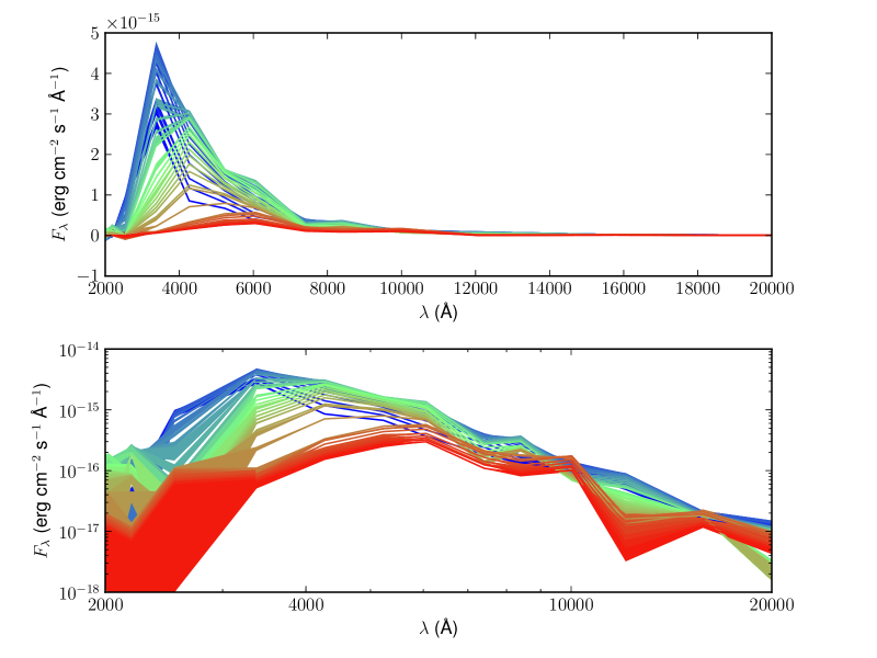
Figure 7: Rest-frame low-resolution SED time series of LSQ12gdj, 1550–23100 Å, constructed from Swift UV + CSP $BVr^{\prime}i^{\prime}$ photometry. SED colours show the phase, ranging from blue ($-10$ days) to red ($+45$ days). Top: linear scale; bottom: log scale. Colored bands represent the 1$\sigma$ confidence region around the mean.

Figure 7 shows the resulting time-dependent SED of LSQ12gdj for zero host galaxy reddening. The peak wavelength changes steadily as the ejecta expand and cool, making Swift $u$ the most luminous band at early phases. Although a significant fraction of the flux is emitted bluewards of 3300 Å, the flux density cuts off sharply bluewards of Swift $uvm2$. Less than 1% of the flux is emitted bluewards of 2300 Å at all epochs, and our SED in these regions is consistent with statistical noise. This behavior is inconsistent with simply being the Rayleigh-Jeans tail of a hot blackbody. Although we have no UV spectroscopy of LSQ12gdj, we expect the sharp cutoff blueward of 3000 Å for the entire rise of the SN to be formed by line blanketing from iron-peak elements (e.g. Cr 2, as in Figure 5), as is common in SNe Ia.

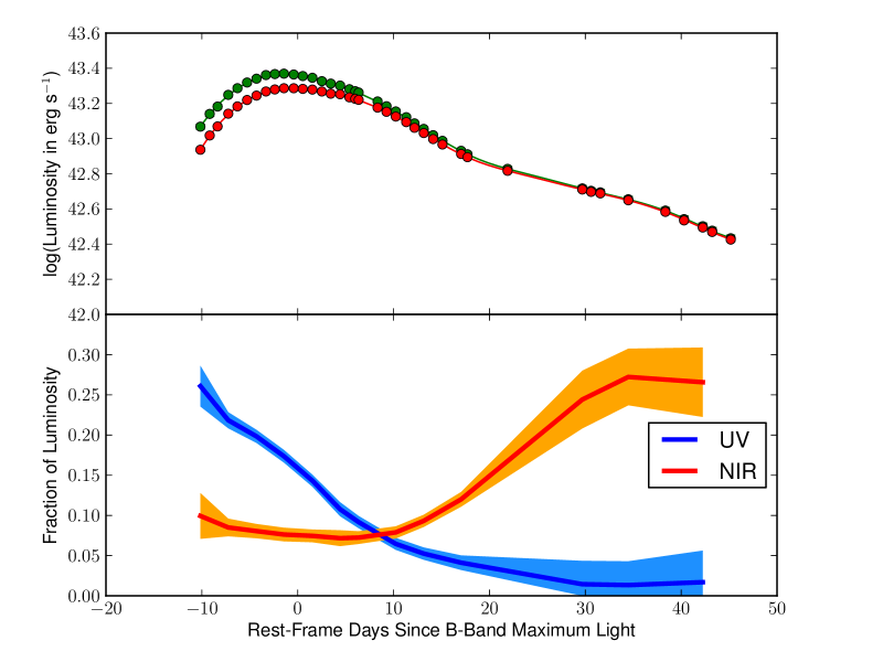
Figure 8: Rest-frame bolometric light curve of LSQ12gdj obtained by integrating the SED of Figure 7. Top: Bolometric light curve 3300–23100 Å (red) and 1550–23100 Å (green) representing the results with and without Swift UV, including Gaussian process regression fit (connecting curves). Bottom: Fraction of bolometric flux bluewards of 3300 Å (“UV”) and redwards of 8800 Å (“NIR”, estimated from a template); the solid curves show the mean behavior, and the lighter bands show the 1$\sigma$ confidence region around the mean.

Figure 8 shows the bolometric light curve, together with Gaussian process regression fits. Like other candidate super-Chandrasekhar-mass SNe Ia observed with Swift (Brown et al., 2014), LSQ12gdj is bright at UV wavelengths from the earliest phases. Up to 27% of the bolometric flux is emitted blueward of 3300 Å at day $-10$, decreasing to 17% at $B$-band maximum light and to $<5\%$ by day $+20$. After day $+20$, the SN is no longer detected in the Swift bands, so the small constant fraction reflects our method of accounting for missing data (with large error bars). For comparison, in the well-observed normal SN Ia 2011fe (Pereira et al., 2013), at most 13% of the luminosity is emitted blueward of 3400 Å, reaching this point 5 days before $B$-band maximum light; the UV fraction is 9% at day $-10$, and only 3% at day $-15$. UV flux contributes only 2% of SN 2011fe’s total luminosity by day +20, and continues to decline thereafter.

Table 6: Ground-based photometry of LSQ12gdj in the natural systems of the Swope and LCOGT telescopes

Phasea	$L_{\mathrm{bol}}^{b}$	$\sigma_{L,\mathrm{stat}}^{c}$	$\sigma_{L,\mathrm{sys}}^{d}$	$\sigma_{L,\mathrm{tot}}^{e}$	$f_{\mathrm{NIR}}^{f}$
(days)	($10^{43}$ erg s-1)	($10^{43}$ erg s-1)	($10^{43}$ erg s-1)	($10^{43}$ erg s-1)
$-10.2$	1.252	0.033	0.025	0.041	0.094
$-9.2$	1.472	0.026	0.029	0.039	0.088
$-8.4$	1.616	0.030	0.032	0.044	0.087
$-7.2$	1.882	0.018	0.037	0.041	0.081
$-6.3$	2.051	0.017	0.041	0.044	0.080
$-5.3$	2.208	0.017	0.044	0.047	0.078
$-4.3$	2.320	0.018	0.046	0.049	0.077
$-3.3$	2.437	0.035	0.048	0.060	0.074

4 PROGENITOR PROPERTIES

In this section we perform some additional analysis to constrain properties of the LSQ12gdj progenitor: the ejected mass, the ${}^{56}\mathrm{Ni}$ mass, and the physical configuration of the CSM envelope (if one is present). We fit the bolometric light curve in §4.1 to infer the ejected mass and place rough constraints on trapped radiation from interaction with a compact envelope. In §4.2 we attempt to constrain the impact of interaction with an extended CSM wind, including constraints on CSM mass based on blueshifted Na 1 D absorption (Maguire et al., 2013) and a light curve comparison to known CSM-interacting SNe Ia. Finally, in §4.3 we consider the implications of our findings for the more established super-Chandrasekhar-mass SNe Ia, including SN 2007if and SN 2009dc.

4.1 Ejected Mass, ${}^{56}\mathrm{Ni}$ Mass, and Trapped Thermal Energy from Interaction with a Compact CSM

LSQ12gdj has excellent UV/optical coverage from well before maximum to over 40 days after maximum, allowing us to model it in more detail than possible for many other SNe Ia. We use the bolomass code (Scalzo et al., in prep), based on a method applied to other candidate super-Chandrasekhar-mass SNe Ia (Scalzo et al., 2010, 2012), as well as normal SNe Ia (Scalzo et al., 2014). The method constrains the ${}^{56}\mathrm{Ni}$ mass, $M_{\mathrm{Ni}}$, and the ejected mass, $M_{\mathrm{ej}}$, using data both near maximum and at late times, when the SN is entering the early nebular phase.

bolomass uses the Arnett (1982) light curve model, including as parameters $M_{\mathrm{Ni}}$ and the expected time $t_{0}$ at which the ejecta become optically thin to ${}^{56}\mathrm{Co}$ gamma rays. However, bolomass also calculates the expected transparency of the ejecta to gamma rays from ${}^{56}\mathrm{Co}$ decay at late times, using the formalism of Jeffery (1999) together with a 1-D parametrized model {$\,\rho(v)$, $\mathbf{X}(v)\,$} of the density and composition structure as a function of the ejecta velocity $v$. The effective opacity for Compton scattering (and subsequent down-conversion) of ${}^{56}\mathrm{Co}$-decay gamma rays in the optically thin limit (Swartz et al., 1995) is much more precisely known than optical-wavelength line opacities near maximum light (Khokhlov et al., 1993); this allows bolomass to deliver robust, quantitative predictions, avoiding uncertainties associated with scaling arguments or assumptions about the optical-wavelength opacity. bolomass uses the affine-invariant Monte Carlo Markov Chain sampler emcee (Foreman-Mackey et al., 2013) to sample the model parameters and marginalize over nuisance parameters associated with systematic errors, subject to a suite of priors which encode physics from contemporary explosion models.

The Arnett (1982) light curve model includes as parameters not only $M_{\mathrm{Ni}}$ and $t_{0}$, but the effects of photon diffusion on the overall light curve shape, the initial thermal energy $E_{\mathrm{th}}$ of the ejecta and the finite size $R_{0}$ of the exploding progenitor. They enter through the dimensionless combinations

$$y\!\! = \!\!\frac{t_{\mathrm{rise}}}{2\tau_{\mathrm{Ni}}}=\frac{t_{\mathrm{rise}}}{17.6~{}\mathrm{days}},$$ (4)

$$w\!\! = \!\!\frac{2R_{0}}{t_{\mathrm{rise}}v_{\mathrm{KE}}}\sim\frac{R_{0}}{10^{15}~{}\mathrm{cm}}.$$ (5)

While $w\ll 1$ for white dwarfs, allowing $w$ to float in this case may help us estimate the contribution of trapped radiation from interaction with a compact, hydrogen-free CSM envelope which might otherwise be invisible; this formalism is not appropriate for an ongoing shock interaction.

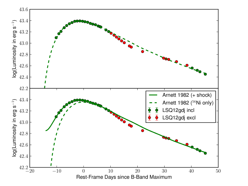
Figure 9: Fits of the Arnett (1982) light curve model to the bolometric light curve of LSQ12gdj, including the trapping of thermalized kinetic energy from an interaction with a compact carbon-oxygen envelope, in the context of the tamped detonation scenario. Top: Zero initial radius. Bottom: Initial radius and thermal energy determined by the fit, showing the full fit (solid curve) and the contribution due only to radioactive decay (dashed curve). Red symbols mark points in the transition regime from photospheric to early nebular phase, which have been excluded from the fit.

Arnett (1982) points out that the assumptions of constant opacity and a sharp photosphere in the expanding SN ejecta break down between maximum light and late phases, when the SN is in transition from full deposition of radioactive decay energy to the optically thin regime. We therefore exclude light curve points between 10 days and 40 days after $B$-band maximum light, and find that the Arnett (1982) light curve model provides an excellent fit ($<1\%$ dispersion) to the remaining points.

The Arnett model also does not treat the ${}^{56}\mathrm{Ni}$ distribution in detail, assuming only that it is centrally concentrated, which prevents it from accurately predicting the light curve shape at very early times (Hachinger et al., 2013; Piro & Nakar, 2013, 2014; Mazzali et al., 2014), as mentioned in §3.2. For example, if LSQ12gdj’s actual rise time is longer than the predictions of our model, the actual ${}^{56}\mathrm{Ni}$ mass could be larger; a 2-day “dark phase” could increase the inferred ${}^{56}\mathrm{Ni}$ mass by up to 25% relative to our estimate. Pinto & Eastman (2000) consider the impact of large amounts of ${}^{56}\mathrm{Ni}$ at high velocities on the light curve: for a uniform ${}^{56}\mathrm{Ni}$ distribution, the lower Compton depth results in a shorter rise time (by as much as 3 days), but also lower $\alpha$ (0.85) as some of the radioactive energy simply leaks out of the ejecta, and these effects roughly balance for our ${}^{56}\mathrm{Ni}$ estimates. More detailed modeling of our spectroscopic time series may provide further information about the true distribution of ${}^{56}\mathrm{Ni}$.

Figure 9 shows two possible fits to the bolometric light curve of LSQ12gdj. When we fix $w=0$ and consider only luminosity from radioactivity, we recover $t_{\mathrm{rise}}=16.4$ days, in agreement with the $t^{2}$ fit to the early-phase LSQ data, and $M_{\mathrm{Ni}}=1.00$ $M_{\odot}$. Allowing $w$ to float reveals a second possible solution, in which trapped thermal energy contributes around 10% of the luminosity at maximum light. The fit has $w=0.013$ and $E_{\mathrm{th}}=6\times 10^{50}$ erg, and has a significantly shorter rise time $t_{\mathrm{rise}}=14.1$ days, exploding just before the initial detection by LSQ. This value of $w$ corresponds to an effective radius of roughly $10^{13}$ cm, more extended than the envelopes in the DET2ENVN series (Khokhlov et al., 1993) but comparable to those predicted by Shen et al. (2012). The amount of thermalized kinetic energy is compatible with the formation of a reverse-shock shell near 10000 $\mathrm{km~{}s}^{-1}$in a tamped detonation or pulsating delayed detonation. Importantly, the trapped radiation contributes most at early times and around maximum light, but disappears on a light curve width timescale, just as suggested by Hachinger et al. (2012) and Taubenberger et al. (2013) in the case of SN 2009dc. The late-time behavior is the same as for the radioactive-only case, and the best-fit ${}^{56}\mathrm{Ni}$ mass is 0.88 $M_{\odot}$. The reduced chi-squares for both fits are very low (0.47 for $w=0$ versus 0.15 for $w>0$), so that while the $w>0$ fit is technically favored, both are consistent with our observations.

The ejected mass estimate depends on the actual density structure and ${}^{56}\mathrm{Ni}$ distribution in the ejecta. We consider two possible functional forms for the density structure, one which depends exponentially on velocity and one with a power-law dependence, as in Scalzo et al. (2014). We parametrize the stratification of the ejecta by a mixing scale $a_{\mathrm{Ni}}$ (Kasen, 2006), and consider stratified cases with $a_{\mathrm{Ni}}=0.1$ and well-mixed cases with $a_{\mathrm{Ni}}=0.5$. The detailed model-dependence of the trapping of radiation near maximum light is often factored out into a dimensionless ratio $\alpha$ (Nugent et al., 1995; Howell et al., 2006, 2009) of order unity, by which the rough “Arnett’s rule” estimate of $M_{\mathrm{Ni}}$ from the maximum-light luminosity is divided. Here we use the Arnett light curve fit directly to estimate the ${}^{56}\mathrm{Ni}$ mass and the amount of thermalized kinetic energy trapped and released, resulting in an effective $\alpha$ between 1.0 and 1.1 for LSQ12gdj. For the $w=0$ Arnett formalism, $\alpha=1$ by construction, ignoring both opacity variation in the ejecta and/or less than complete gamma-ray deposition near maximum light (Blondin et al., 2013). In one-dimensional, Chandrasekhar-mass delayed detonation models (e.g. Khokhlov et al., 1993; Höflich & Khohklov, 1996), a high central density may enhance neutronization near the center of the ejecta, creating a ${}^{56}\mathrm{Ni}$-free “hole”. Some evidence for such a hole is found in late-time spectra of SNe Ia (Höflich et al., 2004; Motohara et al., 2006; Mazzali et al., 2007), and in some multi-dimensional simulations (Maeda et al., 2010a), while other simulations do not support such an effect (Krueger et al., 2012; Seitenzahl et al., 2013). We consider cases both with and without ${}^{56}\mathrm{Ni}$ holes due to neutronization, as in Scalzo et al. (2014). In all reconstructions, we allow the unburned carbon/oxygen fraction, the envelope size, and the thermalized kinetic energy to float freely to reproduce the observed bolometric light curve, including variations in the rise time produced by changes in these parameters.

Table 7: Ejected mass and ${}^{56}\mathrm{Ni}$ mass of LSQ12gdj under various priors

Run	$\rho(v)$a	$a_{\mathrm{Ni}}$b	$v_{\mathrm{KE}}$c ($\mathrm{km~{}s}^{-1}$)	$M_{\mathrm{ej}}/M_{\odot}$d	$P_{\mathrm{SCh}}$e
A	pow3x3	0.5	$10390^{+634}_{-284}$	$1.56^{+0.13}_{-0.08}$	0.992
B	pow3x3	0.1	$10484^{+613}_{-295}$	$1.51^{+0.10}_{-0.07}$	0.953
C	exp	0.5	$10713^{+503}_{-250}$	$1.43^{+0.08}_{-0.05}$	0.691
D	exp	0.1	$10939^{+485}_{-292}$	$1.38^{+0.06}_{-0.07}$	0.354

Table LABEL:tbl:massrecon shows the inferred $M_{\mathrm{ej}}$ and probability of exceeding the Chandrasekhar limit for four different combinations of priors, marginalizing over the full allowed range of $w$ and $E_{\mathrm{th}}$. The full Monte Carlo analysis robustly predicts $t_{\mathrm{rise}}=16\pm 1$ days and $M_{\mathrm{Ni}}=0.96\pm 0.07$ $M_{\odot}$. The thermalized kinetic energy is constrained to be less than about $10^{51}$ erg; this maximum value results in ejecta with a maximum velocity around 10000 $\mathrm{km~{}s}^{-1}$, roughly consistent with our observations. Models which allow ${}^{56}\mathrm{Ni}$ holes shift ${}^{56}\mathrm{Ni}$-rich material to lower Compton optical depths, requiring more massive ejecta to reproduce the late-time bolometric light curves; for LSQ12gdj, this effect is small since the favored super-Chandrasekhar-mass solutions are rapidly rotating configurations with low central density (Yoon & Langer, 2005). If LSQ12gdj in fact had a high central density with corresponding ${}^{56}\mathrm{Ni}$ hole, its ejected mass should be at least 0.1 $M_{\odot}$ higher than what we infer. Since ${}^{56}\mathrm{Ni}$ makes up such a large fraction of the ejecta in any case, there is little difference between the well-mixed models and the stratified models. Models with power-law density profiles have $M_{\mathrm{ej}}$ larger by about 0.14 $M_{\odot}$ than models with exponential density profiles; this is the largest predicted uncertainty in our modeling.

The uncertainty from the unknown ejecta density profile is not easily resolved. Although bolomass can model any user-defined spherically symmetric density structure, the light curve is sensitive primarily to the total Compton scattering optical depth, and not directly to the actual ejecta density profile, except for the most highly disturbed density structures. Scalzo et al. (2014) showed that assuming an exponential density profile led to biases in the reconstructed mass for multi-dimensional explosion models best represented by power laws. Our judgment as to whether LSQ12gdj is actually super-Chandrasekhar-mass thus hinges mostly on which density profile we believe to be more realistic.

If LSQ12gdj is indeed a tamped detonation, it is probably (slightly) super-Chandrasekhar-mass, and could be explained by a Chandrasekhar-mass detonation inside a compact envelope of mass around 0.1 $M_{\odot}$. If all of LSQ12gdj’s luminosity is due to radioactive energy release, it could be (slightly) sub-Chandrasekhar-mass, a good candidate for a double detonation (Woosley & Weaver, 1994; Fink et al., 2010) of about 1.3 $M_{\odot}$, a conventional Chandrasekhar-mass near-pure detonation (Blondin et al., 2013; Seitenzahl et al., 2013), or a pulsating delayed detonation (Khokhlov et al., 1993; Höflich & Khohklov, 1996).

Interestingly, the DDC0 delayed-detonation model of Blondin et al. (2013) has a rise time of 15.7 days, very close to the value we observe. The 1.4-$M_{\odot}$ tamped detonation 1p0_0.4 of Raskin et al. (2014) also comes close to our expected scenario, with a roughly spherical helium envelope that has been thermalized in the merger interaction. The spectra near maximum are blue with shallow features. The envelope is compact, with a density profile following a $r^{-4}$ power law, but could expand to $\sim 10^{13}$ cm if the detonation of the white dwarf primary is delayed after the merger event (Shen et al., 2012).

4.2 Constraints on Ongoing Shock Interaction with an Extended CSM

We also address the question of whether LSQ12gdj might be undergoing shock interaction with a hydrogen-poor extended wind, adding luminosity to its late-time light curve. The “Ia-CSM” events, such as SN 2002ic (Hamuy et al., 2003), SN 2005gj (Aldering et al., 2006; Prieto et al., 2007), SN 2008J (Taddia et al., 2012), and PTF11kx (Dilday et al., 2012), have spectra which seem to be well-fit by a combination of a 1991T-like SN Ia spectrum, a broad continuum formed at the shock front, and narrow H$\alpha$ lines formed in photoionized CSM (Silverman et al., 2013a, b; Leloudas et al., 2013). A hydrogen-poor extended CSM could produce pseudocontinuum luminosity and and weaken absorption lines via toplighting (Branch et al., 2000), while not producing any distinctive line features itself, although a very massive envelope could in principle produce carbon or oxygen lines (Ben-Ami et al., 2014).

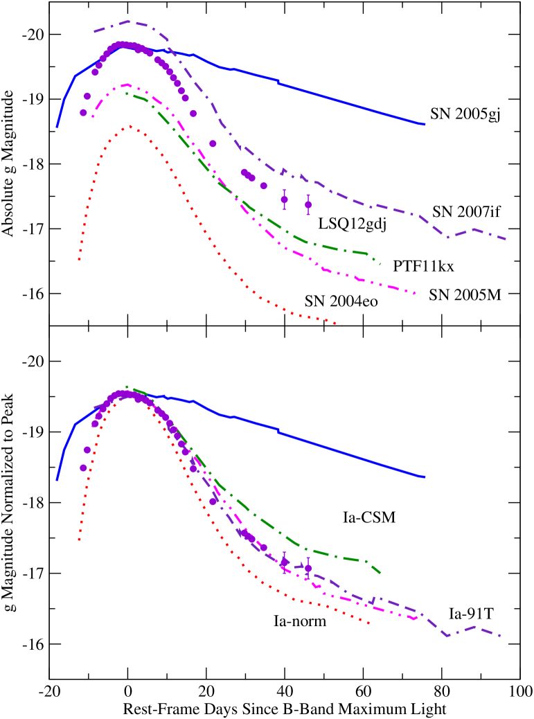
Figure 10: Comparison of $g$-band light curves of peculiar SNe Ia. The CSP and Swift $B$-band light curves of LSQ12gdj (filled circles) have been $S$-corrected to $g$ band using the spectra in this paper. References for the other light curves include: SN 2005gj, from Prieto et al. (2007) (solid curve); PTF11kx, from Dilday et al. (2012) (dash-dot curve); SN 2004eo and SN 2005M, from Contreras et al. (2010) (dotted and dash-dot-dot curves); and SN 2007if, from Stritzinger et al. (2012) and Scalzo et al. (2010) (dash-dash-dot curve).

Figure 10 shows the $g$-band light curve of LSQ12gdj alongside those of the Ia-CSM SN 2005gj and PTF11kx, the super-Chandrasekhar-mass SN 2007if, the 1991T-like SN 2005M, and the fast-declining, spectroscopically normal SN 2004eo. We choose $g$ for the comparison because it is the bluest band observed (or synthesizable) in common for all of the SNe. SN 2005gj, the clearest example of ongoing shock interaction, declines extremely slowly, with far more luminosity at day $+40$ and later than any of the other SNe. PTF11kx, a case of an intermediate-strength shock interaction, has peak brightness comparable to the 1991T-like SN 2005M, but shows a long tail of shock interaction luminosity and is up to 0.5 mag more luminous than SN 2005M at day $+60$. By a year after explosion, the spectrum of PTF11kx, like that of SN 2005gj, is dominated by shock interaction signatures such as H$\alpha$ (Silverman et al., 2013a), rather than by Fe 2 as for SN 2007if (Taubenberger et al., 2013).

Despite having peak magnitudes that differ over a range of 1 mag, SN 2005M, SN 2007if, and LSQ12gdj all have very similar post-maximum light curve shapes, more consistent with each other than with the Ia-CSM. This puts strong constraints on the density and geometry of any CSM present; existing examples of Ia-CSM show that the light curve shapes can vary dramatically according to the density and geometry of the surrounding medium. In particular, none of the SNe Ia-91T show an extended power-law tail to the light curve, nor do they match expectations from radiation hydrodynamics simulations of heavily enshrouded SNe Ia in hydrogen-poor envelopes (Fryer et al., 2010; Blinnikov & Sorokina , 2010).

We can derive a more quantitative upper limit on the presence of extended CSM by searching for circumstellar Na 1 D absorption. Maguire et al. (2013) observed LSQ12gdj with the XSHOOTER spectrograph on the ESO Very Large Telescope at Paranal, finding narrow Na 1 D and Ca 2 H+K absorption blueshifted at $-220$ $\mathrm{km~{}s}^{-1}$ relative to the recessional velocity of the LSQ12gdj host. LSQ12gdj is one of a larger sample of SNe Ia with blueshifted absorption features studied in Maguire et al. (2013). While blueshifted Na 1 D absorption would be expected statistically for a population of progenitors surrounded by a CSM wind, of either single-degenerate (Sternberg et al., 2011) or double-degenerate (Shen et al., 2012; Raskin & Kasen, 2013) origin, we have no way of knowing whether such absorption is circumstellar for any individual SN Ia, or whether it arises from interstellarmaterial in the host galaxy.

We can nevertheless derive a conservative upper limit assuming all of the absorption arises from hydrogen-rich CSM. Since $EW(\mathrm{\text{Na\,\textsc{1}}~{}D)}$ near the host galaxy redshift is small, there should be little CSM present around LSQ12gdj. We use the vpfit code to place an upper limit on the column density of Na 1 using the XSHOOTER spectrum from Maguire et al. (2013), in the case in which all Na 1 D absorption is circumstellar; we obtain $N(\mathrm{\text{Na\,\textsc{1}}})<4\times 10^{11}~{}\mathrm{cm}^{-2}$. For a thin spherical shell of radius $10^{16}$ cm, thickness $10^{14}$ cm, and $H$-rich composition of solar metallicity ($\log(\mathrm{Na/H})+12=6.17$; Asplund et al., 2005) undergoing complete recombination of Na 1, similar to the treatment of SN 2006X in Patat et al. (2007), we obtain a CSM shell mass $M_{\mathrm{env}}<3\times 10^{-7}$ $M_{\odot}$. Similar limits can be obtained by multiplying the upper limit on the hydrogen column density by the surface area of a sphere of radius $10^{16}$ cm ($6\times 10^{-7}$ $M_{\odot}$), or by using the estimated fluence of ionizing photons from Patat et al. (2007) ($6\times 10^{-7}$ $M_{\odot}$). The known H-rich SNe Ia-CSM, such as SN 2005gj, have estimated electron densities and CSM masses several orders of magnitude higher (Aldering et al., 2006), as do the total CSM masses ejected in the tidal tails of the mergers simulated by Raskin & Kasen (2013).

These estimates, of course, assume hydrogen-rich CSM, whereas shock-powered models for super-Chandrasekhar-mass SNe Ia posit CSM rich in helium or even carbon (Hachinger et al., 2012; Taubenberger et al., 2013). The first ionization potentials for carbon (11.3 eV) and oxygen (13.6 eV) are comparable to that of hydrogen, so one might expect similar electron densities from photoionization in those cases; however, the expected relative abundance of sodium in such material is highly uncertain, making it difficult to set definite limits. For helium the ionization potential is much higher (24.6 eV), requiring hard UV flux blueward of 500 Å; this entirely precludes useful limits from Na 1 D absorption for CSM composed predominantly of helium.

To summarize, we have compiled the following lines of evidence regarding CSM interaction in LSQ12gdj:

1. Since LSQ12gdj is clearly typed as a SN Ia near maximum light, any CSM by this time either must be optically thin or must not cover the entire photosphere. The fraction of luminosity which can be produced by shock heating or other non-radioactive sources is limited to about 75% of the total (Leloudas et al., 2013).

2. The weak Na 1 D absorption limits the mass of extended hydrogen-rich CSM around LSQ12gdj to be less than $\sim 10^{-6}$ $M_{\odot}$.

3. An extended all-helium or carbon-oxygen CSM could in theory evade the Na 1 D constraints, but would probably produce a lingering power-law tail to the light curve, as in SN 2005gj or PTF11kx, which we do not see in LSQ12gdj.

4. Fits to the bolometric light curve of LSQ12gdj limit the size of any compact envelope to be $<10^{13}$ cm. In this case the interaction would be frozen out before the first detection, resulting in all intermediate-mass elements being swept up into a reverse-shock shell and producing the very low velocity gradient observed.

5. If LSQ12gdj has a compact envelope, its relatively high Si 2 velocity implies a light envelope of mass $\sim 0.1$ $M_{\odot}$; this traps some radiation, but not as much as might be trapped in a heavily enshrouded explosion.

It seems therefore that while some CSM may be present around LSQ12gdj, luminosity from ongoing shock interaction is negligible. Without tell-tale emission lines, however, the composition of the CSM and the evidence for a single-degenerate origin for LSQ12gdj remain ambiguous.

4.3 Implications for SN 2007if and SN 2009dc

LSQ12gdj was flagged early in its evolution as a bright, peculiar SN Ia. By considering the UV contribution to LSQ12gdj’s luminosity, we have shown that up to 10% of LSQ12gdj’s maximum-light luminosity may be trapped thermal energy from an interaction with a compact envelope. Such a model, with small variations in the relative contributions of ${}^{56}\mathrm{Ni}$ mass and radioactivity to the maximum-light luminosity, can explain the observational appearance of 1991T-like SNe Ia of comparable luminosity, including SN 1991T itself and the SNe Ia analyzed in Scalzo et al. (2012).

We now consider what lessons may extend to the much brighter SNe Ia, SN 2007if and SN 2009dc, if any. While Taubenberger et al. (2011), Hachinger et al. (2012), and Taubenberger et al. (2013) considered a number of possible physical scenarios for SN 2009dc, they were led to present a white dwarf exploding inside an envelope as the most likely scenario based on the following considerations: The abundance patterns derived from photospheric-phase and nebular-phase spectra are characteristic of the thermonuclear explosion of a white dwarf, rather than of a core-collapse event. A single rapidly rotating white dwarf with the necessary mass ($>2M_{\odot}$) and inferred ${}^{56}\mathrm{Ni}$ mass would have been difficult to explain from the standpoint of binary star evolution. Violent mergers or collisions in double-degenerate systems are expected to produce highly asymmetric explosions, while the lack of continuum polarization implies a spherically symmetric event (Tanaka et al., 2010). Requiring that the event be spherical also rules out models which explain SN 2009dc’s luminosity mainly through viewing angle effects (Hillebrandt et al., 2007). Finally, even those channels able to produce very large ${}^{56}\mathrm{Ni}$ masses, such as white dwarf collisions (Raskin et al., 2010; Kushnir et al., 2013), produce ejecta velocities which are too high to match the observations. An interaction with an envelope converts kinetic energy into luminosity, enabling a powerful explosion to have low ejecta velocity (Scalzo et al., 2010) and potentially relaxing the requirement of a very high ${}^{56}\mathrm{Ni}$ mass.

However, Hachinger et al. (2012) and Taubenberger et al. (2013) make no specific predictions for the geometry or physics of the interaction. Hachinger et al. (2012) show that spectra of SN 2009dc can be reproduced by the sum of a SN Ia spectrum and a smooth pseudocontinuum; they consider polynomials and spectra of SNe with strong CSM interactions as possible functional forms. The interaction luminosity is simply assumed to be the difference between what is observed and what is predicted from radioactive decay. Taubenberger et al. (2013) examine the influence of the post-interaction ejecta density profile on radiation trapping at late times, and estimate a CSM mass of about 0.6 $M_{\odot}$; they make few predictions about the CSM geometry necessary to reproduce the near-maximum light curve, and raise concerns about fine-tuning.

Using LSQ12gdj as a point of departure, we can reason about how the presence of interaction luminosity affects inferences about the ejected masses and ${}^{56}\mathrm{Ni}$ masses of SN 2007if and SN 2009dc. While ongoing interactions may run into fine-tuning problems, an interaction can contribute to maximum-light luminosity while leaving the late-time light curve undisturbed as long as the envelope is sufficiently compact.

The influence of interaction with a compact envelope can thus be crudely estimated as an adjustment to the luminosity-to-radioactivity ratio $\alpha$. The Scalzo et al. (2010) analysis of SN 2007if used $\alpha=1.3\pm 0.1$, i.e., it assumed that around 30% of SN 2007if’s maximum-light luminosity was trapped radiation, and a long rise time of 23 days. While the rising part of the light curve was well-sampled by ROTSE-III (Yuan et al., 2010), with the first detection at 20 days before $B$-band maximum light, SN 2007if has only one pre-maximum bolometric light curve point, making its maximum-light colour uncertain (Scalzo et al., 2012) and precluding a more detailed analysis of the pre-maximum light curve. Crucially, SN 2007if also has no UV data. If the UV component of SN 2007if’s bolometric luminosity evolved in a similar way to LSQ12gdj’s, this would have made SN 2007if 17% more luminous at peak ($3.7\times 10^{43}$ erg s^-1), requiring a ${}^{56}\mathrm{Ni}$ mass of around ($2.0/\alpha$) $M_{\odot}$. Most of the trapped radiation should be gone around 60 days after explosion, so the late-time light curve measurements correctly reflect that the ejecta must have been extremely massive. If we assume $\alpha=2.0$, bringing $M_{\mathrm{Ni}}$ down to 1.0 $M_{\odot}$, the limit of what can be achieved in a Chandrasekhar-mass explosion (Khokhlov et al., 1993), we must still have $M_{\mathrm{ej}}>2.26$ $M_{\odot}$ at 99% confidence.

Similar considerations apply to SN 2009dc, which has an almost identical light curve to SN 2007if out to 100 days past maximum light. SN 2009dc also has Swift data (Silverman et al., 2011), though none before maximum light, so the precise shape of its pre-maximum bolometric light curve is still subject to large uncertainties. At maximum light, Silverman et al. (2011) estimate that about 20% of SN 2009dc’s bolometric flux is emitted in the UV, similar to LSQ12gdj. The low absorption-line velocities make it impossible for SN 2009dc to have a “normal” density structure, or even much burned material beyond about 9000 $\mathrm{km~{}s}^{-1}$. For SN 2009dc to have been a tamped detonation or pulsating delayed detonation, the outer, incompletely burned layers of ejecta must have represented a much larger fraction of the total ejecta mass — possibly as high as 30% of the total — in order to reproduce its even lower ejecta velocities. Under these conditions, the reverse shock should penetrate far into the inner layers of ejecta before stalling, and the distribution of material in the reverse-shock shell becomes important to gamma-ray transport at late times. Thus the approximation previously used by Scalzo et al. (2012) for SN 2007if and other super-Chandrasekhar-mass candidates, in which the shock redistributes kinetic energy and traps thermal energy but has little effect on the late-time light curve, probably breaks down for SN 2009dc. Detailed hydrodynamic simulations of explosions inside compact envelopes could be used to suggest a suitable density profile.

In contrast to SN 2007if, SN 2009dc’s relatively large ($\sim 75$ $\mathrm{km~{}s}^{-1}$ day^-1) Si 2 velocity gradient presents a problem for explosion scenarios which produce shell structures in the ejecta (Quimby et al., 2007), because no velocity plateau is evident. It is also clear that intermediate-mass elements cannot all be trapped in a thin layer, as with the delayed detonation scenario suggested by Childress et al. (2013a) for SN 2012fr. However, given the strength of the shock necessary, the approximation of the reverse-shock shell as a thin layer could also break down here. A pulsating delayed detonation could have given SN 2009dc a highly disturbed density structure without the need for an envelope or for a very narrow layer of intermediate-mass elements in velocity space. Baron et al. (2012) invoked such a model for the slow-declining SN 2001ay (Krisciunas et al., 2011).

One difficulty with pulsating models for SN 2007if and SN 2009dc is that, while the pulsation will thermalize and redistribute kinetic energy, the shock freezes out much sooner after explosion than in the case of a tamped detonation. This forces $w=0$ and prevents a significant contribution of trapped thermalized kinetic energy to the maximum-light luminosity (but potentially further enhancing trapping of radioactive energy near maximum light).

5 Conclusions

LSQ12gdj is a well-observed, overluminous SN Ia in a nearby galaxy with little to no dust extinction. The extensive spectroscopic time series show that LSQ12gdj is spectroscopically 1991T-like, with intermediate-mass element absorption signatures only in a narrow range of velocities, much like SN 2007if and other 1991T-like SNe Ia Scalzo et al. (2010, 2012). From the bolometric light curve of LSQ12gdj we infer a ${}^{56}\mathrm{Ni}$ mass of about 1.0 $M_{\odot}$ and an ejected mass near the Chandrasekhar mass.

Observations at UV wavelengths well before maximum light provide additional useful constraints on the properties of LSQ12gdj and other 1991T-like SNe Ia, not considered elsewhere. A large fraction (17%) of the bolometric luminosity near maximum light, and nearly 30% in the earliest observations, is emitted bluewards of 3300 Å. Accounting for this effect increases the derived ${}^{56}\mathrm{Ni}$ mass significantly relative to cases in which it is ignored (e.g., Scalzo et al., 2012), assuming that the SN is powered through radioactivity alone.

Our excellent time and wavelength coverage also allow us to consider alternative sources of luminosity for LSQ12gdj, which can guide our intuition for other luminous super-Chandrasekhar-mass SN Ia candidates. We find that as much as 10% of LSQ12gdj’s luminosity could come from trapped thermal energy from an early-phase shock interaction, with virtually none coming from ongoing shocks at later times. Such a mechanism could in principle explain the extreme luminosities and low photospheric velocities of SN 2007if and SN 2009dc as resulting from the trapping of thermalized kinetic energy from a short interaction at early times, without appealing to ongoing shock interactions with extended winds which are likely to cause greater deviations from SN Ia behavior than observed.

Our findings represent what can be done with detailed observations, and to push our understanding of super-Chandrasekhar-mass SNe Ia forward, even more detailed observations will be needed. Early ultraviolet coverage is critical, starting as soon after explosion as possible. Optical and near-infrared observations extending to late times, well past maximum light, are needed to place helpful constraints on the mass. Nebular spectra can elucidate the density structure of the innermost ejecta, with implications for the importance of radiation trapping near maximum light. These observations must go hand in hand with sophisticated, self-consistent modelling which can deal with theoretical uncertainties and with systematic errors in the observations.

Measurement of the properties of a general spectroscopically selected sample of 1991T-like SNe Ia could provide vital clues to the identity of their progenitors and how they relate to other super-Chandrasekhar-mass SNe Ia, such as SN 2006gz and SN 2009dc, and to CSM-interacting SNe Ia, such as SN 2005gj and PTF11kx. Leloudas et al. (2013) show a strong association between 1991T-like SNe Ia and the growing Ia-CSM subclass which show narrow H$\alpha$ lines in their spectra (Silverman et al., 2013b); they imply that 1991T-like SNe Ia must in general be single-degenerate explosions, although not all of them are required to display strong CSM interaction. Similarly, a SN Ia sample from an untargeted search selected only by peak absolute magnitude can determine the spectroscopic diversity and range of explosion mechanisms which can account for superluminous SNe Ia, and how many superluminous SNe Ia result from the explosions of super-Chandrasekhar-mass white dwarfs.

References

- (1)
- Ade et al. (2013) Ade, P. A. R., Aghanim, N., Armitage-Caplan, C., et al. 2013, arXiv:1303.5076
- Aldering et al. (2006) Aldering, G., Antilogus, P., Bailey, S., et al. 2006, ApJ, 650, 510
- Arnett (1982) Arnett, W. D. 1982, ApJ, 253, 785
- Asplund et al. (2005) Asplund, M., Grevesse, N., & Sauval, A. J. 2005, in Cosmic Abundances as Records of Stellar Evolution and Nucleosynthesis, ed. F. N. Bash, & T. G. Barnes, p. 25
- Bailey et al. (2009) Bailey, S., Aldering, G., Antilogus, P., et al. 2009, A&A, 500, L17
- Baltay et al. (2013) Baltay, C., Rabinowitz, D., Hadjiyska, E., et al. 2013, PASP, 125, 683
- Baron et al. (2012) Baron, E., Höflich, P., Krisciunas, K., et al. 2012, ApJ, 753, 105
- Ben-Ami et al. (2014) 2014, ApJ, 785, 37
- Benetti et al. (2005) Benetti, S., Cappellaro, E., Mazzali, P., et al. 2005, ApJ, 623, 1011
- Bertin & Arnouts (1996) Bertin, E. & Arnouts, S. 1996, A&AS, 317, 393
- Bertin et al. (2002) Bertin, E., Mellier, Y., Radovich, M., et al. 2002, ASP Conference Series, Vol. 281, eds. D.A. Bohlender, D. Durand, & T.H. Handley, p. 228.
- Blinnikov & Sorokina (2010) Blinnikov, S. I. & Sorokina, E. I. 2010, arXiv:1009.4353
- Blondin & Tonry (2007) Blondin, S., & Tonry, J. L. 2007, ApJ, 666, 1024
- Blondin et al. (2013) Blondin, S., Dessart, L., Hillier, D. J., et al. 2013, MNRAS, 429, 2127
- Branch et al. (1993) Branch, D., Fisher, A., & Nugent, P. 1993, AJ, 106, 2383
- Branch et al. (2000) Branch, D., Jeffery, D. J., Blaylock, M., et al. 2000, PASP, 112, 217
- Branch et al. (2006) Branch, D., Dang, L., Hall, N., et al. 2006, PASP, 118, 560
- Branch et al. (2007) Branch, D., Troxel, M. A., Jeffery, D. J., et al. 2007, PASP, 119, 135
- Branch et al. (2008) Branch, D., Jeffery, D. J., Parrent, J., et al. 2008, PASP, 120, 135
- Breeveld et al. (2011) Breeveld, A. A., Landsman, W., Holland, S. T., et al. 2011, in AIP Conf. Proc. 1358, Gamma-Ray Bursts 2010, ed. J. E. McEnery, J. L. Racusin, & N. Gehrels (Melville, NY: AIP), 373; arXiv:1102.4717
- Brown et al. (2009) Brown, P., Holland, S., Immler, S., et al. 2009, AJ, 137, 4517
- Brown et al. (2014) Brown, P., Holland, S., & Milne, P. 2014, ApJ, 787, 29
- Burns et al. (2014) Burns, C., Stritzinger, M., Phillips, M. M., et al. 2014, ApJ, in press (arXiv:1405.3934)
- Cardelli et al. (1988) Cardelli, J. A., Clayton, G. C. & Mathis, J. S. 1988, ApJ, 329, L33
- Cellier-Holzem et al. (2012) Cellier-Holzem, F., Canto, A., Antilogus, P., et al. 2012, ATEL #4566
- Childress et al. (2013a) Childress, M., Scalzo, R. A., Sim, S. A., et al. 2013, ApJ, 770, 29
- Childress et al. (2013b) Childress, M. 2014, Ap&SS, 349, 617
- Conley et al. (2008) Conley, A., Sullivan, M., Hsiao, E. Y., et al. 2008, ApJ, 681, 482
- Contreras et al. (2010) Contreras, C., Hamuy, M., Phillips, M. M. 2010, AJ, 139, 519
- Das & Mukhopadhyay (2013a) Das, U. & Mukhopadhyay, B. 2013, Phys. Rev. Lett., 110, 071102
- Das & Mukhopadhyay (2013b) Das, U. & Mukhopadhyay, B. 2013, ApJ, 767, L14
- Dilday et al. (2012) Dilday, B., Howell, D. A., Cenko, S. B., et al.2012, Science, 337, 942
- Di Nella et al. (1996) Di Nella, H., Couch, W. J., Paturel, G., et al. 1996, MNRAS, 283, 367
- Di Stefano & Kilic (2012) Di Stefano, R. & Kilic, M. 2012, ApJ, 759, 56
- Fink et al. (2010) Fink, M., Röpke, F. K., Hillebrandt, W., et al. 2010, A&A, 514, A53
- Filippenko et al. (1992) Filippenko, A. V., Richmond, M. W., Matheson, T., et al. 1992, ApJ, 384, L15
- Folatelli et al. (2010) Folatelli, G., Phillips, M. M., Burns, C., R., et al. 2010, AJ, 139, 120
- Foley & Kasen (2011) Foley, R. J. & Kasen, D. 2010, ApJ, 729, 55
- Foreman-Mackey et al. (2013) Foreman-Mackey, D., Hogg, D. W., Lang, D., et al. 2013, PASP, 125, 306
- Fryer et al. (2010) Fryer, C. L., Ruiter, A. J., Belczynski, K., et al. 2010, ApJ, 725, 296
- Fukugita et al. (2010) Fukugita, M., Ichikawa, T., Gunn, J. E., et al. 1996, AJ, 111, 1748
- Ganeshalingam et al. (2011) Ganeshalingam, M., Li, W., & Filippenko, A. V. 2011, MNRAS, 416, 2607
- Goldhaber et al. (2001) Goldhaber, G., Groom, D. E., Kim, A. G., et al. 2001, ApJ, 558, 359
- Guy et al. (2007) Guy, J., Astier, P., Baumont, S., et al. 2007, A&A, 466, 11
- Guy et al. (2010) Guy, J., Sullivan, M., Conley, A., et al. 2010, A&A, 523, 7
- Hachinger et al. (2012) Hachinger, S., Mazzali, P., Taubenberger, S., et al. 2012, MNRAS, 427, 2057
- Hachinger et al. (2013) Hachinger, S., Mazzali, P., Sullivan, M., et al. 2013, MNRAS, 429, 2228
- Hachisu et al. (2011) Hachisu, I., Kato, M., Saio, H., et al. 2012, ApJ, 744, 69
- Hamuy et al. (2003) Hamuy, M., Phillips, M. M., Suntzeff, N., et al. 2003, Nature, 424, 651
- Hamuy et al. (2006) Hamuy, M., Folatelli, G., Morrell, N. I., et al. 2006, PASP, 118, 2
- Hicken et al. (2007) Hicken, M., Garnavich, P. M., Prieto, J. L., et al. 2007, ApJ, 669, L17
- Hillebrandt et al. (2007) Hillebrandt, W., Sim, S. A., & Röpke, F. K. 2007, A&A, 465, L17
- Höflich & Khohklov (1996) Höflich, P. & Khohklov, A. 1996, ApJ, 457, 500
- Höflich et al. (2004) Höflich, P., Gerardy, C., Nomoto, K., et al. 2004, ApJ, 617, 1258
- Howell et al. (2006) Howell, D. A., Sullivan, M., Nugent, P. E., et al. 2006, Nature, 443, 308
- Howell et al. (2009) Howell, D. A. et al. 2009, ApJ, 691, 661
- Iben & Tutukov (1984) Iben, I. & Tutukov, A. V. 1984, ApJS, 54, 335
- Jeffery (1999) Jeffery, D. J. 1999, arXiv:astro-ph/9907015
- Justham (2011) Justham, S. 2011, ApJ, 730, L34
- Kasen (2006) Kasen, D. 2006, ApJ, 649, 939
- Khokhlov et al. (1993) Khokhlov, A., Müller, E. & Höflich, P. 1993, A&A, 270, 223
- Krisciunas et al. (2011) Krisciunas, K., Li, W., Matheson, T., et al. 2011, AJ, 142, 74
- Krueger et al. (2012) Krueger, B. K. Jackson, A. P., Townsley, D. M., et al.2012, ApJ, 757, 175
- Kushnir et al. (2013) Kushnir, D., Katz, B., Dong, S., et al. 2013, ApJ, 778, L37
- Landolt (1992) Landolt, A. U. 1992, AJ, 104, 340
- Lantz et al. (2004) Lantz, B., Aldering, G., Antilogus, P., et al. 2004, Proc. SPIE, 5249, 146
- Leloudas et al. (2013) Leloudas, G., Hsiao, E. Y., Johansson, J., et al. 2013, A&A, submitted (arXiv:1306.1549)
- Maeda et al. (2009) Maeda, K., Kawabata, K., Li, W., et al. 2009, ApJ, 690, 1745
- Maeda et al. (2010a) Maeda, K., Röpke, F., Fink, M., et al. 2010, ApJ, 712, 624
- Maeda et al. (2010b) Maeda, K., Benetti, S., Stritzinger, M., et al. 2010, Nature, 466, 7302
- Maeda et al. (2011) Maeda, K., Leloudas, S., Taubenberger, S., et al. 2011, MNRAS, 413, 3075
- Maguire et al. (2013) Maguire, K., Sullivan, M., et al. 2013, MNRAS, 436, 222
- Mazzali et al. (2007) Mazzali, P. A., Roepke, F., Benetti, S., et al. 2007, Science, 315, 825
- Mazzali et al. (2014) Mazzali, P. A., Sullivan, M., Hachinger, S., et al. 2014, MNRAS, 439, 1959
- Motohara et al. (2006) Motohara, K., Maeda, K., Gerardy, C. L., et al. 2006, ApJ, 652, L101
- Nomoto et al. (1984) Nomoto, K., Thielemann, F.-K., & Yokoi, K. 1984, ApJ, 286, 644
- Nugent et al. (1995) Nugent, P., Branch, D., Baron, E., et al. 1995, Phys. Rev. Lett., 75, 394
- Nugent et al. (2002) Nugent, P. E., Kim, A. G., & Perlmutter, S. 2002, PASP, 114, 803
- Patat et al. (2007) Patat, F., Chandra, P., Chevalier, R., et al. 2007, Science, 317, 924
- Pedregosa et al. (2011) Pedregosa, F., Varoquaux, G., Gramfort, A., et al. 2011, JMLR, 12, 2825
- Pereira et al. (2013) Pereira, R., Aldering, G., Antilogus, P. 2013, A&A, 554, 27
- Perlmutter et al. (1999) Perlmutter, S., Aldering, G., Goldhaber, G., et al. 1999, ApJ, 517, 565
- Pfannes et al. (2010b) Pfannes, J. M. M. Niemeyer, J., & Schmidt, W. 2010, A&A, 509, 75
- Phillips et al. (1992) Phillips, M. M., Wells, L. A., Suntzeff, N. B., et al. 1992, AJ, 103, 1632
- Phillips et al. (1999) Phillips, M. M., Lira, P., Suntzeff, N. B., et al. 1999, AJ, 118, 1766
- Pinto & Eastman (2000) Pinto, P. & Eastman, R. 2000, ApJ, 530, 744
- Piro & Nakar (2013) Piro, A. L., & Nakar, E. 2013, ApJ, 769, 67
- Piro & Nakar (2014) Piro, A. L., & Nakar, E. 2014, ApJ, 784, 85
- Prieto et al. (2007) Prieto, J., Garnavich, P., Phillips, M. M., et al.2007, arXiv:0706.4088
- Quimby et al. (2007) Quimby, R., Höflich, P., & Wheeler, J. C. 2007, ApJ, 666. 1083
- Raskin et al. (2010) Raskin, C., Scannapieco, E., Rockefeller, G., et al. 2010, ApJ, 724, 111
- Raskin & Kasen (2013) Raskin, C., & Kasen, D. 2013, ApJ, 772, 1
- Raskin et al. (2014) Raskin, C., Kasen, D., Moll, R., et al. 2014, ApJ, 788, 75
- Rasmussen & Williams (2006) Rasmussen, C. E. & Williams, C. K. I., 2006, Gaussian Processes for Machine Learning, MIT Press
- Riess et al. (1996) Riess, A. G., Press, W. H., & Kirshner, R. P. 1996, ApJ, 473, 88
- Riess et al. (1998) Riess, A. G., Filippenko, A. V., Challis, P., et al. 1998, AJ, 116, 1009
- Riess et al. (1999) Riess, A. G., Filippenko, A. V., Li, W., et al. 1999, AJ, 118, 2675
- Scalzo et al. (2010) Scalzo, R. A., Aldering, G., Antilogus, P., et al. 2010, ApJ, 713, 1073
- Scalzo et al. (2012) Scalzo, R. A., Aldering, G., Antilogus, P., et al. 2012, ApJ, 757, 12
- Scalzo et al. (2014) Scalzo, R. A., Aldering, G., Antilogus, P., et al. 2014, MNRAS, in press (arXiv:1402:6842)
- Schlafly & Finkbeiner (2011) Schlafly, E. F., & Finkbeiner, D. P. 2011, ApJ, 737, 103
- Seitenzahl et al. (2013) Seitenzahl, I., Ciaraldi-Schoolmann, F., Röpke, F. K., et al. 2013, MNRAS, 429, 1156
- Shen et al. (2012) Shen, K., Bildsten, L., Kasen, D., et al. 2012, ApJ, 748, 35
- Silverman et al. (2011) Silverman, J. M. et al. 2011, MNRAS, 410, 585
- Silverman et al. (2012) Silverman, J. M. et al. 2012, MNRAS, 425, 1789
- Silverman et al. (2013a) Silverman, J. M., Nugent, P., Gal-Yam, A., et al. 2013, ApJ, 772, 125
- Silverman et al. (2013b) Silverman, J. M., Nugent, P., Gal-Yam, A., et al. 2013, ApJS, 207, 3
- Stetson (1987) Stetson, P. B. 1987, PASP, 99, 191
- Sternberg et al. (2011) Sternberg, A., Gal-Yam, A., Simon, J. D., et al. 2011, Science, 333, 856
- Stritzinger et al. (2012) Stritzinger, M., Phillips, M. M., Boldt, L., et al. 2011, AJ, 142, 156
- Swartz et al. (1995) Swartz, D. A., Sutherland, P. G., & Harkness, R. P. 1995, ApJ, 446, 766
- Taddia et al. (2012) Taddia, F., Stritzinger, M. D., Phillips, M. M., et al. 2012, A&A, 545, 7
- Tanaka et al. (2010) Tanaka, M., Kawabata, K., Yamanaka, M., et al. 2010, ApJ, 714, 1209
- Taubenberger et al. (2011) Taubenberger, S., Benetti, S., Childress, M. et al. 2011, MNRAS, 412, 2735
- Taubenberger et al. (2013) Taubenberger, S., Kromer, M., Hachinger, S. et al. 2013, MNRAS, 432, 3117
- Tody (1993) Tody, D. 1993, Astronomical Data Analysis Software and Systems II, 52, 173
- Thomas et al. (2011) Thomas, R. C., Nugent, P. E., & Meza, J. C. 2011, PASP, 123, 237
- Tripp (1998) Tripp, R. 1998, A&A, 331, 815
- Wang et al. (2009) Wang, X., Filippenko, A. V., Ganeshalingam, M., et al. 2009, ApJ, 699, L139
- Woosley & Weaver (1994) Woosley, S. E. & Weaver, T. A. 1994, ApJ, 423, 371
- Yamanaka et al. (2009) Yamanaka, M., Kawabata, K., Kinugasa, K., et al. 2009, ApJ, 707, L118
- Yaron & Gal-Yam (2012) Yaron, O., & Gal-Yam, A. 2012, PASP, 124, 668
- Yoon & Langer (2005) Yoon, S.-C. & Langer, N. 2005, A&A, 435, 967
- Yuan et al. (2010) Yuan, F., Quimby, R. M., Wheeler, J. C., et al. 2010, ApJ, 715, 1338