Relativistic Positioning Systems: Numerical Simulations

Abstract

The motion of satellite constellations similar to GPS and Galileo is numerically simulated and, then, the region where bifurcation (double positioning) occurs is appropriately represented. In the cases of double positioning, the true location may be found using additional information (angles or times). The zone where the Jacobian, J, of the transformation from inertial to emission coordinates vanishes is also represented and interpreted. It is shown that the uncertainties in the satellite world lines produce positioning errors, which depend on the value of $|J|$. The smaller this quantity the greater the expected positioning errors. Among all the available 4-tuples of satellites, the most appropriate one –for a given location– should minimize positioning errors (large enough $|J|$ values) avoiding bifurcation. Our study is particularly important to locate objects which are far away from Earth, e.g., satellites.

1 General considerations

Global Navigation Satellite Systems (GNSSs) are satellite constellations broadcasting signals, which may be used to find the position of a receiver (user) [7]. GNSSs are mainly used to locate receivers on Earth surface. In this case, users receiving signals from four or more satellites may be always located with admissible positioning errors. However, if the user to be located is far away from Earth, two main problems may arise, the first one is the existence of two possible positions for the object (bifurcation), some previous considerations about this problem may be found in [1, 3, 10]. The second problem is related to the positioning errors due to uncertainties in the world lines of the satellites. These errors are proved to be too big for some user positions close to points where the Jacobian $J$ –of the transformation from inertial to emission coordinates– is too small. In this paper, we find and represent the regions where the above problems arise. Only numerical calculations may be used to find these regions in the case of realistic GNSSs. Moreover, their representation is an additional problem, which have been solved by choosing appropriate sections –of the 4D emission region– and by using suitable methods previously developed in other research fields (see below). The mentioned regions have been only studied in the interior of a big sphere having a radius of $10^{5}\ km$, which is centred in a point E of the Earth surface (see Fig. 1).

Quantities $G$, $M_{\oplus}$, $t$, and $\tau$ stand for the gravitation constant, the Earth mass, the coordinate time, and the proper time, respectively. Greek (Latin) indexes run from $0$ to $3$ ($1$ to $3$). Quantities $\eta_{\alpha\beta}$ are the covariant components of the Minkowski metric tensor. Our signature is (+,+,+,–). The unit of distance is assumed to be the Kilometre, and the time unit is chosen in such a way that the speed of light is $c=1$. The index $A$ numerates the four satellites necessary for relativistic positioning.

GPS and GALILEO satellite constellations are simulated [14, 15]. Satellite trajectories are assumed to be circumferences in the Schwarzschild space-time created by an ideal spherically symmetric Earth. A first order approximation in $GM_{\oplus}/R$ is sufficient for our purposes. The angular velocity is $\Omega=(GM_{\oplus}/R^{3})^{1/2}$, and coordinate and proper times are related as follows: $\gamma=\frac{dt}{d\tau}=(1-\frac{3GM_{\oplus}}{R})^{-1/2}\ .$ Angles $\theta$ and $\phi$ fix the orbital plane (see [15]), and the angle $\alpha_{A}(\tau)=\alpha_{A0}-\Omega\gamma\tau$ localizes the satellite on its trajectory. This simple model is good enough as a background configuration. Deviations with respect to the background satellite world lines will be necessary to develop our study about positioning accuracy (see below).

Other known world lines (no circumferences) of Schwarzschild space-time might be easily implemented in the code, but the new background satellite configurations would lead to qualitatively comparable numerical results; at least, for the problems considered in this paper.

The angle $\alpha_{A}(\tau)$ may be calculated for every $\tau$, and the two angles fixing the orbital plane ($\theta$ and $\phi$) are constant. From these three angles and the proper times $\tau^{A}$, the inertial coordinates of the four satellites, $x^{\alpha}_{A}$, may be easily found to first order in $GM_{\oplus}/R$ [15]. This means that the world lines of the background satellites [functions $y^{\alpha}=x^{\alpha}_{A}(\tau^{A})$] are known for every satellite $A$. Hence, given the emission coordinates $(\tau^{1},\tau^{2},\tau^{3},\tau^{4})$ of a receiver, the inertial coordinates $x^{\alpha}_{A}\equiv(x_{A},y_{A},z_{A},t_{A})$ of the four satellites –at emission times– may be easily calculated. The knowledge of the satellite world lines is necessary for positioning; namely, to find the inertial coordinates from the emission ones [4].

The satellite world lines are also necessary to go from the inertial coordinates of an user to its emission ones. This transformation is now considered under the assumption that photons move in the Minkowski space-time, whose metric has the covariant components $\eta_{\alpha\beta}$. This approach is good enough for us. Since photons follow null geodesics from emission to reception, the following algebraic equations must be satisfied:

$$\eta_{\alpha\beta}[x^{\alpha}-x^{\alpha}_{A}(\tau^{A})][x^{\beta}-x^{\beta}_{A}(\tau^{A})]=0\ .$$ (1)

These four equations must be numerically solved to get the four emission coordinates $\tau^{A}$. The four proper times are the unknowns in the system (1), which may be easily solved by using the well known Newton-Raphson method [13]. Since the satellite world lines are known, functions $x^{\alpha}_{A}(\tau^{A})$ may be calculated for any set of proper times $\tau^{A}$, thus, the left hand side of Eqs. (1) can be computed and, consequently, the Newton-Raphson method may be applied. A code has been designed to implement this method. It requires multiple precision. Appropriate tests have been performed [15].

Moreover, given four emission coordinates $\tau^{A}$, Eqs. (1) could be numerically solved to get the unknowns $x^{\alpha}$, that is to say, the inertial coordinates (positioning); however, this numerical method is not used. It is better the use of a certain analytical formula giving $x^{\alpha}$ in terms of $\tau^{A}$, which was derived in [4]. The analytical formula is preferable because of the following reasons: (i) the numerical method based on Eqs. (1) is more time consuming and, (ii) the analytical formulation of the problem allows us a systematic and clear discussion of bifurcation, and also a study of the positioning errors close to points of vanishing Jacobian.

The analytical formula [4] has been described in various papers [4, 7, 5, 15], and numerically applied in [14, 15]. This formula involves function $\chi^{2}$, which is the modulus of the configuration vector, and a discriminant $\Delta$. The definitions of both $\chi^{2}$ and $\Delta$ may be found in [4, 7, 6]. It is very important that these two quantities may be calculated by using only the emission coordinates $\tau^{A}$. From the analytical formula giving the inertial coordinates in terms of the emission ones, and taking into account some basic relations of Minkowski space-time, the following propositions have been previously proved [4, 5, 7]:

(a) For $\chi^{2}\leq 0$, there is only a positioning (past-like) solution.

(b) For $\chi^{2}>0$ there are two positioning solutions; namely, there are two sets of inertial coordinates (two physical real receivers) associated to the same emission coordinates $\tau^{A}$.

(c) The Jacobian $J$ of the transformation giving the emission coordinates in terms of the inertial ones vanishes if and only if the discriminant $\Delta$ vanishes.

(d) The Jacobian $J$ may only vanish if $\chi^{2}>0$; namely, in the region of double positioning (bifurcation).

(e) The Jacobian $J$ may only vanish if the lines of sight –at emission times– of the four satellites belong to the same cone (with vertex in the user).

These conclusions are basic for the numerical estimations and discussions presented below. In particular, after calculating $\chi^{2}$ and $\Delta$ from the emission coordinates, propositions (a) and (b) allow us to find the regions where bifurcation takes place, whereas the zones with vanishing Jacobian (infinite positioning errors) may be found by using proposition (c).

2 Emission region

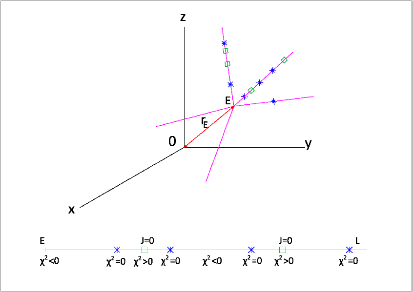
Figure 1: 3D sections ($t=constant$) of the emission region are considered. Point E is an arbitrary centre. Its distance to the origin $O$ is the Earth radius. $L$ is the distance from E to another point of the section. 3072 segments starting from E and having distinct directions cover each 3D section. Along each direction our study is restricted to $0<L<L_{max}=10^{5}\ km$. We look for the zeros of $\chi^{2}$ and $J$. The Jacobian only may vanish in the segments where $\chi^{2}>0$, which are limited by the first and second or by the third and fourth $\chi^{2}$-zeros.

For every set of four satellites, the so-called 4D emission region [4, 7, 15] is studied by considering 3D sections $t=constant$. Each of these sections is covered by points according to the method described in Fig. 1. Let us here give some additional details. Healpix package –first used in cosmic microwave background researches [11]– is used to define 3072 directions. A segment with one of its ends at $E$ and having length $L_{max}=10^{5}\ km$ is associated to each direction. A great enough number of points are uniformly distributed along every direction. The inertial coordinates of the chosen points are known by construction; then, the Newton-Raphson method –implemented in our numerical codes– gives the associated emission coordinates, which allow us the computation of $\chi^{2}$ and $\Delta$ (see section 1). With these quantities, we may find the zeros of both $\chi^{2}$ and $J$ [proposition (c) of section 1] along any given direction. As it is displayed in Fig. 1, various zeros of $\chi^{2}$ and $J$ may be found in each direction. They may be distributed in different ways by obeying proposition (d) of section 1.

Once the zeros of $\chi^{2}$ and $\Delta$ have been found for all the Healpix directions (3072), an appropriate method is necessary to display the results. Our method is based on the Healpix pixelisation and the mollwide projection (see [15] for more details). Healpix associates a pixel to each direction. The pixel colour measures the value of some chosen quantity according to the colour bar displayed in our figures, which are mollwide projections of the pixelised sphere.

The structure of the 3D section considered in Fig. 2 ($t=25\ h$ after the time origin) is displayed in seven panels. The blue pixels of panel (a) show the directions of the four chosen satellites when they emitted the signals received at point E. Since satellite velocities are much smaller than the speed of light, the satellite positions at emission times are very similar for every point of the 3D section under consideration. In order to understand panels (b)–(h) the reader need to know the quantity associated to every colour bar and the meaning of the grey pixels. In panel (b) [(e)], the colour bar shows the distance from $E$ to the first zero of $\chi^{2}$ [$J$], and along the directions corresponding to the grey pixels, function $\chi^{2}$ [$J$] does not vanish, at least, up to a distance $L_{max}$ from $E$. In panel (c) [(f)], the colour bar gives the distance from the first to the second zero of $\chi^{2}$ [$J$], and function $\chi^{2}$ [$J$] does not vanish two times in the directions of the grey pixels (up to $L_{max}$) and, finally, in panel (d) [(g)] the colour bar displays distances from the second to the third zero of $\chi^{2}$ [$J$], and no a third zero of $\chi^{2}$ [$J$] has been found along the directions of the grey pixels (up to $L_{max}$). In some cases, there are no directions with more than one zero of functions $\chi^{2}$ (see [15]) and $J$. In any case, panels (c)–(g) of Fig. 2 show that there are only few directions with two zeros of these functions, and also that directions with three zeros are very scarce. Other 3D sections and other 4-tuples of satellites have been studied with similar results.

From Figs. (1) and (2), it follows that the emission region has the following structure: there are directions without zeros of $\chi^{2}$ and $J$. These directions subtend a great solid angle [grey pixels of panel. (b) and (e)]. The complementary solid angle corresponds to directions with one or more zeros of $\chi^{2}$. From point E to the first zero of $\chi^{2}$ there is no bifurcation, but it appears beyond the first zero. For the small number of directions having a second zero, there is no bifurcation beyond this zero, but it occurs again beyond the third zero (see Fig. 1), which only exists for very scarce directions. We have verified that, according to proposition (d) of section 1, the Jacobian only vanishes in regions with bifurcation.

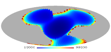
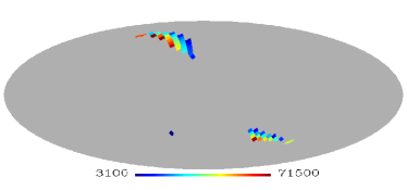
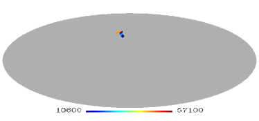
(a)
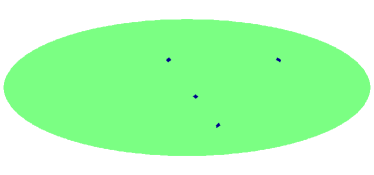
(b) (e)
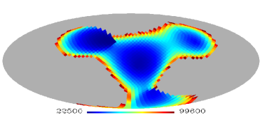
(c) (f)
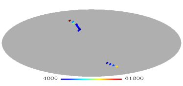
(d) (g)

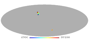
Figure 2: Structure of section $x^{4}=t=25\ h$ for $L<10^{5}\ km$

3 Positioning errors and satellite uncertainties

Figure 3: Estimator $\Delta_{d}$ (in $km$) against the distance $L$ to $E$ (in $Mm\equiv 10^{3}km$) along the chosen direction in a $200\ km$ interval centred at a point where $J=0$. Close to this point, quantity $\Delta_{d}$ takes on very large values

The background world lines of the satellites are the circumferences of section 1, whose equations have the form $y^{\alpha}=x^{\alpha}_{A}(\tau^{A})$. Let us first suppose that the background world lines are exactly followed by the satellites (without uncertainties). Under this assumption, given the inertial coordinates $x^{\alpha}$ of an user, the background world line equations, Eqs. (1), the Newton-Raphson method, and multiple precision may be used to find the emission coordinates $\tau^{1},\tau^{2},\tau^{3},\tau^{4}$ with very high accuracy. Finally, the chosen inertial coordinates $x^{\alpha}$ may be recovered from the emission ones –with very high accuracy– by using the analytical solution derived in [4]. This process is useful to prove that our numerical codes work with high accuracy.

Let us now suppose that there are uncertainties in the satellite world lines, whose equations are $y^{\alpha}=x^{\alpha}_{A}(\tau^{A})+\xi^{\alpha}_{A}$, where $\xi^{\alpha}_{A}$ are deviations with respect to the background world lines due to known or unknown external actions on the satellites. Let us now take the above inertial coordinates $x^{\alpha}$, the equations $\eta_{\alpha\beta}[x^{\alpha}-x^{\alpha}_{A}(\tau^{A})-\xi^{\alpha}_{A}][x^{\beta}-x^{\beta}_{A}(\tau^{A})-\xi^{\beta}_{A}]=0$, the Newton-Raphson method, and multiple precision, to get the perturbed emission coordinates [$\tau^{1}+\Delta(\tau^{1}),\tau^{2}+\Delta(\tau^{2}),\tau^{3}+\Delta(\tau^{3}),\tau^{4}+\Delta(\tau^{4})$]. Since the time deviations $\Delta(\tau^{A})$ are all small, quantities $\xi^{\alpha}_{A}$ may be assumed to be constant in the short interval [$\tau^{A},\tau^{A}+\Delta(\tau^{A})$]. Finally, by using the analytical solution mentioned above, new inertial coordinates $x^{\alpha}+\Delta(x^{\alpha})$ may be obtained from the emission coordinates $\tau^{A}$ and the deviations $\xi^{\alpha}_{A}$. Coordinates $x^{\alpha}+\Delta(x^{\alpha})$ are to be compared with the inertial coordinates $x^{\alpha}$ initially assumed.

Quantity $\Delta_{d}=[\Delta^{2}(x^{1})+\Delta^{2}(x^{2})+\Delta^{2}(x^{3})]^{1/2}$ is a good estimator of the positioning errors produced by the assumed uncertainties, $\xi^{\alpha}_{A}$, in the satellite motions.

For a certain direction, we have taken an interval of $200\ km$ centred at a zero of function $J$ and, then, quantity $\Delta_{d}$ has been calculated in 200 uniformly distributed points of the chosen interval. In each of these points, the same deviations $\xi^{\alpha}_{A}$ have been used to perturb the satellite world lines. The three quantities $\xi^{i}_{A}$ have been written in terms of the modulus $\Xi_{A}=[(\xi^{1}_{A})^{2}+(\xi^{2}_{A})^{2}+(\xi^{3}_{A})^{2}]^{1/2}$ and two angles $\Theta$ and $\Phi$ (spherical coordinates) and, then, quantities $\Xi_{A}$, $\Theta$, $\Phi$, and $\xi^{4}_{A}$ have been generated as random uniformly distributed numbers in the intervals [$0,10^{-3}$] in $km$, [$0,\pi$], [$0,2\pi$], and [$0,10^{-3}$] in time units (see section 1), respectively. Results are presented in Fig. 3, where we see that our estimator of the positioning errors $\Delta_{d}$ is very large close to the central point where $J=0$. This fact is important in section 4 (satellite positioning). It is due to the fact that the satellite to be located may cross the region of vanishing $J$.

The Jacobian is being numerically calculated –in any point of the emission region– to perform a relativistic study of the so-called dilution of precision [12]; namely, to look for the relation between the geometry of the system satellites-user and the amplitude of the positioning errors. This study must be developed for users on Earth, as well as for users far away from Earth (satellites).

4 Looking for the position of a satellite

(h)
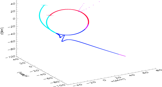
(i)

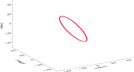
Figure 4: Top: positioning a Galileo satellite with four GPS emitters. Bottom: same for a GPS satellite and four Galileo emitters.

In this paper, we are concerned with the location of users which move far away from Earth as, e.g., an user in a satellite. Of course, we use the emission times broadcast by four satellites, which might belong, e.g., to GPS or Galileo GNSSs. Two particular cases are considered. In the first (second) one, the user travels in a Galileo (GPS) satellite and the emitters are four GPS (Galileo) satellites. Thus, the world lines of the user and the emitters are known (see section 1). As it follows from section 2, there is no bifurcation for distances to $E$ smaller than about $10^{4}\ km$, which means that GPS and Galileo satellites, which have altitudes of $20200$ and $23222\ km$, may pass from a regions with bifurcation to other region with single positioning or vice versa. The parts of the user circumference where bifurcation occurs are now determined in the two cases. Results of the first (second) case are presented in panel (h) [(i)] of Fig. (4).

7200 equally spaced points are considered on the user world line. In each point, the emission coordinates are calculated (Newton-Rhapson) and, from them, the sign of $\chi^{2}$ is found, this sign tell us if the point is single valued or it has an associated false position (bifurcation). Single valued points are red and are always located on the user circumference.

Four sets of 1800 points have been selected and –in the case of bifurcation– these sets have been ordered in the sense of growing time (dextrogyre) by using the following sequence of colours: black, fuchsia, dark blue and light blue.

Initial points may be: a single valued red point (represented by a star) or a bifurcation represented by two black stars.

Since GPS and GALILEO satellites have not the same period, the final point has not always the same $\chi^{2}$ sign as the initial one. In the case of bifurcation one of the points is on the circumference and the other point is an external light blue star.

In the transition from red (single positioning) to any other colour (bifurcation), one of the positions is on the circumference and the other one tends to infinity. The same occurs from any colour (bifurcation) to red (single positioning). Any other colour change is continuous. It is due to the fact that we have decided to change the colour to follow the satellite motion.

In panel (i) of Fig. (4), there are no bifurcation at all (red points). This is an exceptional case. A more frequent situation with zones of bifurcation is given in panel (h), where the asymptotic behaviour at the ends of the bifurcation intervals is displayed.

5 General discussion

In our approach, satellites move in Schwarzschild space-time, so the effect of the Earth gravitational field on the clocks is taken into account, e.g., it has been verified that GPS clocks run more rapid than clocks at rest on Earth by about 38.4 microseconds per day. This prediction agrees with previous ones, which strongly suggests that our methods and codes work.

Since the Earth gravitational field produces a very small effect on photons while they travel from the satellites to the receiver (the covered distance is not large and the gravitational field is weak), photons have been moved in Minkowski space-time.

We are currently moving photons in Schwarzschild, Kerr, and PPN space-times; however, only small corrections arise with respect to the approach assumed here. Previous work on this subject has been performed in various papers [8, 9, 2].

In this paper, the emission coordinates are calculated, from the inertial ones, by using accurate numerical codes based on the Newton-Raphson method. However, the inertial coordinates are obtained, from the emission ones (positioning), by means of the analytical transformation law derived in [4].

From the emission coordinates and the satellite world lines, one easily finds the number of possible receiver positions. If this number is two, there is bifurcation. In this case, it has been proposed a method (based on angle measurements) to select the true position [7]. Other methods (based on time measurements) are possible (see [15]).

We have proved that small uncertainties in the satellite world lines produce large positioning errors if $J\simeq 0$. A more detailed study of this type of errors is in progress.

The emission region has been studied for a certain 4-tuple of satellites. The zones with bifurcation and those having small values of $|J|$ have been found, and appropriate methods have been used to their representation. We have seen that satellites moving at altitudes greater than about $10^{4}\ km$ may cross these zones, which leads to problems due to bifurcation and large positioning errors. In a GNSS there are various 4-tuples of satellites which may be used to find the position of a certain user. Among the possible 4-tuples without bifurcation, we should choose the 4-tuple leading to the greatest value of $|J|$ to minimize positioning errors.

Positioning on Earth surface is always single ($\chi^{2}\leq 0$) and the Jacobian does not vanish in this case. Hence, our study is particularly relevant in the case of users moving far away from Earth.

Acknowledgments This work has been supported by the Spanish Ministries of Ciencia e Innovación and Economía y Competitividad, MICINN-FEDER projects FIS2009-07705 and FIS2012-33582.

References

- [1] J. S. Abel and J. W. Chaffee. Existence and uniqueness of gps solutions. IEEE Transactions on Aerospace and Electronic Systems, 27(6):952–956, 1991.
- [2] D. Bunandar S.A. Caveny and R.A. Matzner. Measuring emission coordinates in a pulsar-based relativistic positioning system. Phys. Rev. D, 84:104005–9p, 2011.
- [3] J. W. Chaffee and J. S. Abel. On the exact solutions of the pseudorange equations. IEEE Transactions on Aerospace and Electronic Systems, 30(4):1021–1030, 1994.
- [4] B. Coll J.J. Ferrando and J.A. Morales-Lladosa. Positioning systems in Minkowski space-time: from emission to inertial coordinates. Class. Quantum Grav., 27:065013–17p, 2010.
- [5] B. Coll J.J. Ferrando and J.A. Morales-Lladosa. From emission to inertial coordinates: an analytical approach. J. Phys. Conf. Ser., 314:012105–4p, 2011.
- [6] B. Coll J.J. Ferrando and J.A. Morales-Lladosa. From inertial to emission coordinates: splitting of the solution relatively to an inertial observer. submitted to Acta Futura, 2012.
- [7] B. Coll J.J. Ferrando and J.A. Morales-Lladosa. Positioning systems in Minkowski space-time: Bifurcation problem and observational data. Phys. Rev. D, 86:084036–10p, 2012.
- [8] A. Čadež U. Kostić and P. Delva. Mapping the spacetime metric with a global navigation satellite system. Advances in Space Research, Final Ariadna Report 09/1301, Advanced Conceps Team. European Space Agency:1–61, 2010.
- [9] P. Delva U. Kostić and A. Čadež. Numerical modeling of a global navigation satellite system in a general relativistic framework. Advances in Space Research, 47:370–379, 2011.
- [10] E.W. Grafarend and J. Shan. A closed-form solution of the nonlinear pseudo-ranging equations (gps). ARTIFICIAL SATELLITES, Planetary Geodesy, 31(3):133–147, 1996.
- [11] K.M. Gòrski E. Hivon and B.D. Wandelt. Analysis issues for large cmb data sets. In Proc. of the MPA/ESO Conference on Evolution of Large Scale Structure. Ipscam, Enschede, pages 37–42, 1999.
- [12] R.B. Langley. Dilution of precision. GPS World, 10(5):52–59, 1999.
- [13] W.H. Press S.A. Teukolski W.T. Vetterling and B.P. Flannery. Numerical recipes in fortran 77: the art of scientific computing. Cambridge University Press, New York, pages 355–362, 1999.
- [14] N. Puchades and D. Sáez. From emission to inertial coordinates: a numerical approach. J. Phys. Conf. Ser., 314:012107–4p, 2011.
- [15] N. Puchades and D. Sáez. Relativistic positioning: four-dimensional numerical approach in Minkowski space-time. Astrophys. Space Sci., 341:631–643, 2012.