Magnetic field induced phases in anisotropic triangular antiferromagnets: application to $\mathrm{CuCrO_{2}}$

Abstract

We introduce a minimal spin model for describing the magnetic properties of $\mathrm{CuCrO_{2}}$. Our Monte Carlo simulations of this model reveal a rich magnetic field induced phase diagram, which explains the measured field dependence of the electric polarization. The sequence of phase transitions between different mutiferroic states arises from a subtle interplay between spatial and spin anisotropy, magnetic frustration and thermal fluctuations. Our calculations are compared to new measurements up to 92 T.

Triangular lattice antiferromagnets (TLA) are widely studied in the field of frustrated magnetism. Complex orderings and rich phase diagrams arise because three antiferromagnetic interactions within a triangle cannot be simultaneously satisfied. Delafossite CuCrO₂ is a particularly clean example of a TLA where quasi-classical Cr³⁺ $S=3/2$ spins form a triangular lattice in the $ab$ plane. Kadowaki et al. (1990); Crottaz et al. (1996) The spins have out-of-plane anisotropy and weak interlayer coupling that is one to two orders of magnitude smaller than the in-plane interactions. Poienar et al. (2010); Frontzek et al. (2011); Vasiliev et al. (2013) The three spins of each triangle form a nearly 120^∘ structure and all three sublattices form proper-screw spirals that propagate along the same [110] axis with propagation vector $q=0.329$ (the spins rotate in and out of the $ab$ plane).  Kadowaki et al. (1990); Soda et al. (2009, 2010) The spiral can propagate along any of six directions (three choices for the [110] axis and two choices for the helicity) leading to six possible domains.

The proper-screw spiral induces an electric polarization ${\bf P}$ along the spiral propagation vector. Kimura et al. (2008); Seki et al. (2008); Kimura et al. (2009a); Soda et al. (2009); Poienar et al. (2009, 2010); Soda et al. (2010); Kajimoto et al. (2010) This allows us to probe phase transitions between spiral states at high applied magnetic fields $\mathbf{H}_{a}$, while the magnetization is largely insensitive to these transitions. The non-zero ${\bf P}$ is consistent with Arima’s mechanism for multiferroic behavior,  hisa Arima (2007) where the spiral magnetic structure slightly influences the hybridization between the Cr $d$-orbitals and the O $p$-orbitals via spin-orbit coupling, creating a net ${\bf P}\parallel{\bf q}$. Thus, a pattern of electromagnetic domains forms below the magnetic ordering temperature that can be influenced by small electric and magnetic fields relative to the dominant exchange interactions. Kimura et al. (2009a); Soda et al. (2009)

The triangular layers of CuCrO₂ stack along the $c$-axis such that a Cr³⁺ ion from one layer lies at the center of a triangle of Cr³⁺ ions in the next layer. Kadowaki et al. (1990); Crottaz et al. (1996); Seki et al. (2008) The triangular lattice distorts by about 0.01% as a result of the spiral magnetic ordering, leading to two different exchange interactions, $J$ and $J^{\prime}$, along different bonds of the triangle Kimura et al. (2009b, a); Poienar et al. (2009, 2010); Aktas et al. (2013) (Fig. 1). Thermodynamic measurements show two close-lying phase transitions. Elastic neutron diffraction measurements suggest that below $T_{N}=24.2$ K, the triangular plane develops collinear spin correlations. A spiral long-range order appears below $T_{\mathrm{MF}}=23.6$ K and also induces net $\mathbf{P}$, possibly via a first-order transition. Kimura et al. (2008); Ehlers et al. (2013); Aktas et al. (2013)

The ${\bf H}_{a}$ dependence of this spiral ordering is only partially explored in experiments and theory. Fishman (2011); Kimura et al. (2008); Seki et al. (2008); Mun et al. (2014) For applied magnetic fields along [110] and $H_{a}>5.3$ T, the proper screw spiral flops into a cycloidal spiral with the same ${\bf q}$ vector.  Kimura et al. (2008); Soda et al. (2009); Kimura et al. (2009a); Soda et al. (2010); Yamaguchi et al. (2010) Since there are six possible domains with different spiral propagation axes, the flop only occurs in the two domains that have their propagation axis perpendicular to the applied magnetic field. During the spin flop, the electric polarization of those domains rotates from being perpendicular to being parallel to ${\bf H}_{a}$. This cycloidal spiral phase persists beyond 65 T. Mun et al. (2014) While the phase diagram for ${\bf H}_{a}\parallel ab$ contains only one phase transition at 5.3 T (in the explored region of phase space up to 65 T), the phase diagram for ${\bf H}_{a}\parallel{\hat{c}}$ contains a series of field-induced phases. Mun et al. (2014) For certain temperatures, the sequence of phase transitions leads to an oscillation in the magnitude of ${\bf P}$ as a function of $H_{a}$. Mun et al. (2014)

Because ${\bf P}$ is induced by a magnetic spiral in $\mathrm{CuCrO_{2}}$, it is interesting to know the magnetic structure of the new phases. We note that these phases are not captured by recent calculations for $\mathrm{CuCrO_{2}}$. Fishman (2011) Here we present a minimal model that applies to $\mathrm{CuCrO_{2}}$, along with new measurements of ${\bf P}$ in CuCrO₂ up to 92 T. Our Monte Carlo (MC) simulations reproduce the zero-field spiral magnetic order and capture the essentials of the field-induced phase diagrams along different magnetic field directions. Four key competing ingredients are important in this problem: frustration, thermal fluctuations, spatially anisotropic exchange interactions and spin anisotropy. Although the spin anisotropy and spatial distortion are weak, they are always relevant perturbations because the ground state of the frustrated Heisenberg model is highly degenerate.

To build a minimal model for $\mathrm{CuCrO_{2}}$ we note that the Cr³⁺ $S=3/2$ spins are large enough to be treated classically, and that the new phases found in Ref. Mun et al. (2014) occur at relatively high temperature $T$. In addition, the low field spiral plane is perpendicular to $[110]$ and the electric polarization flop transition depends weakly on the in-plane field direction, indicating a weak in-plane hard-axis anisotropy. Finally, the ordered moment is maximal along $[001]$, implying that this is the easy-axis. Frontzek et al. (2011, 2012) Based on these facts and the small spatial anisotropy (see Fig. 1), we introduce the following 2D model Hamiltonian for $\mathrm{CuCrO_{2}}$

$$\mathcal{H}=\sum_{<ij>}J_{{ij}}\mathbf{S}_{i}\cdot\mathbf{S}_{j}+\sum_{i}\left[\frac{1}{2}A_{x}S_{i,x}^{2}-\frac{1}{2}A_{z}S_{i,z}^{2}-\mathbf{H}\cdot\mathbf{S}_{i}\right],$$ (1)

where ${\bf H}\equiv g\mu_{B}{\bf H}_{a}$ ($\mu_{B}$ is Bohr magneton and $g\simeq 2$ is the $g$-factor), $J$ and $J^{\prime}$ are the AFM nearest neighbor (NN) interaction. The single-ion anisotropy terms are much weaker than the dominant exchange interactions, $0<A_{x},\ A_{z}\ll J_{ij}$, and ${\bf S}_{j}$ is a classical unit vector representing the spin at site $j$. We have chosen the $z$-axis along $[001]$ and the $x$ and $y$ axes along $[110]$ and $[1\bar{1}0]$, respectively (see Fig. 1).

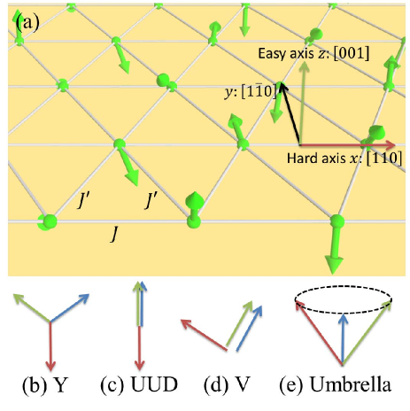
Figure 1: (color online) (a) Schematic view of the Hamiltonian in Eq. (1). (b-e) Typical spin configurations in a unit triangle. The Y state can be either commensurate (CY) or incommensurate with the lattice (ICY), while the umbrella state is always incommensurate (ICU) for $|J-J^{\prime}|\ll J$. The UUD and V states are always commensurate with the lattice.

Besides the fully-polarized state, four other spin states are stabilized in different regions of the phase diagram of $\mathcal{H}$ (see Fig. 1). For spatially-isotropic exchange interaction ($J^{\prime}=J$) with easy-axis spin anisotropy, the so-called “Y” state becomes stable at low magnetic fields. Miyashita (1986) The (up-up-down) UUD state, with net magnetization equal to $1/3$ of the saturation value, becomes stable above a critical field $H_{c}\simeq J/3$. Upon further increasing $H$, there is another transition to the so-called “V” state that remains stable until the spins become fully polarized. For a spatially anisotropic interaction ($J^{\prime}\neq J$) without spin anisotropy, the incommensurate non-coplanar umbrella state has lower energy than the Y phase at low fields because of its higher uniform magnetic susceptibility. Griset et al. (2011) Besides the UUD state stabilized by thermal fluctuations at high temperatures, the umbrella state occupies most of the $H-T$ phase diagram. Here we show that the combined effects of spin and spatial anisotropies in Eq. (1) reproduce the measured phase diagrams of $\mathrm{CuCrO_{2}}$ for both measured field orientations.

Table 1: Coplanarity $K$ and vector charity parallel (perpendicular) to the magnetic field $\chi_{\parallel}$ ($\chi_{\perp}$) in different magnetic states.

	ICY	ICU	CY	CU	UUD	V
$K$	$=0$	$=0$	$>0$	$>0$	$=0$	$>0$
$\chi_{\parallel}$	$=0$	$>0$	$=0$	$>0$	$=0$	$=0$
$\chi_{\perp}$	$>0$	$=0$	$>0$	$=0$	$=0$	$=0$

To discriminate between the competing spin orderings shown in Fig. 1, we introduce the spin co-planarity Watarai et al. (2001)

$$K^{2}=|\mathbf{K}_{12}^{2}|+|\mathbf{K}_{23}^{2}|+|\mathbf{K}_{31}^{2}|,$$ (2)

where $K_{ij}=(\mathbf{m}_{i}\times\mathbf{m}_{j})\times\mathbf{H}/H$ and $\mathbf{m}_{i}$ is the sublattice magnetization. Note that $K$ vanishes for incommensurate ordering because $\mathbf{m}_{i}$ is parallel to ${\bf H}$ and also vanishes for the UUD phase because the moments are collinear. To discriminate between possible $K=0$ phases, we also introduce the vector chirality Griset et al. (2011)

$$\mathbf{\chi}=\frac{2}{3\sqrt{3}L^{2}}\sum_{r}\left[\mathbf{S}_{r}\times\mathbf{S}_{r+\delta_{1}}+\mathbf{S}_{r+\delta_{1}}\times\mathbf{S}_{r+\delta_{2}}+\mathbf{S}_{r+\delta_{2}}\times\mathbf{S}_{r}\right],$$ (3)

where $\mathbf{S}_{r}$ and $\mathbf{S}_{r+\delta_{i}}$ ($i=1,2$) are spins in the same triangle. We compute the components parallel ($\chi_{\parallel}$) and perpendicular ($\chi_{\perp}$) to $\mathbf{H}$. As shown in Table 1, the combined order parameters $K$ and $\chi$ allow us to identify each of the competing spin orderings.

A big system size is required to capture the very small deviation of $q$ from the commensurate value ($q=0.329$) that is observed in $\mathrm{CuCrO_{2}}$. Soda et al. (2009) Given the limitations in system sizes that are accessible for numerical simulations, we use a slightly smaller value of $q=0.3125$ (corresponding to $J^{\prime}/J=0.7654$) in our MC simulations. $A_{z}=0.05J$ and $A_{x}=0.005J$ are typical parameters for the single-ion anisotropy terms. Details of the numerical calculation are provided in Ref. SI .

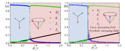
Figure 2: (color online) (a) Different observables as a function of ${\bf H}\parallel{\hat{y}}$ obtained from equilibrium simulations. (b) Similar to (a) but obtained by sweeping the magnetic field. Here $T=0.02J$ and $M_{y}$ is the total magnetization along the field direction.

We first focus on the case $\mathbf{H}\parallel\hat{y}$ shown in Fig. 2 (a). $\chi_{\parallel}$ increases sharply at $H_{y}/J\simeq 0.8$ indicating a first-order phase transition from the incommensurate Y state to the IC umbrella state ($K=0$ indicates incommensurability). However, the magnetization curve only shows a practically unnoticeable discontinuity at the transition. This spin flop transition can be understood as follows. Small distortions of the spin configuration can be neglected for a weak spin anisotropy. For hard-axis anisotropy along the $x$ direction, the spins in the ICY state lie in the $yz$ plane and the spin configuration for the ICY ground state is $\mathbf{S}=[0,\ \cos(qx),\ \sin(qx)]$. The corresponding energy is $E_{Y}=-A_{z}/2-\chi_{Y}H^{2}/2-J-J^{\prime 2}/2J$, where $\chi_{Y}={J^{3}}{(2J+J^{\prime})^{-2}}{(2{J^{2}}-2JJ^{\prime}+J{{}^{\prime 2}})^{-1}}$ is the magnetic susceptibility. The spins cannot avoid the hard axis in the umbrella state: $\mathbf{S}=[\cos\theta\cos(qx),\ \cos\theta\sin(qx),\ \sin\theta]$, and its energy is $E_{U}=\frac{1}{2}\left(A_{x}-A_{z}\right)\cos^{2}\theta-\chi_{U}H^{2}/2-J-J^{\prime 2}/2J$ with $\chi_{U}=J{(2J+J^{\prime})^{-2}}$ being the uniform magnetic susceptibility and $\sin\theta=HJ(2J+J^{\prime})^{-2}$. The Y and umbrella states have the same energy in absence of spatial and spin anisotropies regardless of the field value. Because thermal fluctuations favor collinear or coplanar states, Shender (1982); Henley (1989) the Y state is selected at finite $T$. For $|J-J^{\prime}|/J\ll 1$, the umbrella state has higher magnetic susceptibility: $\Delta\chi\equiv\chi_{U}-\chi_{Y}={(J-J^{\prime})^{2}}/9{J^{3}}$. Thus, the umbrella state can be stabilized at high fields if the difference in the Zeeman energy gain outweighs the energy loss due to hard-axis anisotropy. The spin-flop transition field is estimated as $H_{f,y}=3J\sqrt{A_{x}J}/|J-J^{\prime}|$ when $A_{x},A_{z}\ll 9(J-J^{\prime})^{2}/J$. The resulting transition field is about $H_{f,y}\approx 0.9J$, which is close to the value of $H_{f,y}=0.81J$ obtained from simulations [Fig. 2(a)]. The discrepancy arises from the fact that the spin ordering is not a pure single-${\bf q}$ state. SI The spin-flop transition has to overcome the weak hard-axis anisotropy. Thus the hysteresis of this transition should also be weak. We performed additional simulations by sweeping $H$ gradually, SI and the results are shown in Fig. 2 (b). Hysteresis is absent in agreement with our experimental observations. Note also that the UUD state is absent at low $T$. The phase diagram for $\mathbf{H}\parallel\hat{y}$ is depicted in Fig. 4 (a). The weak $T$-dependence of the transition field is also consistent with the experiments.

Next we describe the case ${\bf H}\parallel{\hat{z}}$. The results for the order parameters and magnetization are displayed in Fig. 3(a). Several phase transitions are observed as a function of $H_{z}$. The low-field ICY state undergoes a transition into the ICU state. A second transition into the CY state occurs before reaching the UUD state. The V state is stabilized immediately above the UUD plateau. Finally, the ICU state reappears at higher fields and remains stable until the spins become fully saturated. Except for the transition from the CY to UUD state, the transitions are strongly first order, according to the hysteresis in magnetic-sweep simulations. The UUD phase exists even at low temperatures because $H$ is now parallel to the easy-axis. The first transition from the ICY to ICU state can again be understood from simple energetic considerations. The energy of the Y state is the same as for ${\bf H}\parallel{\hat{y}}$. The energy of the umbrella phase is ${E_{U}}={\cos^{2}}\theta{A_{x}}/2-A_{z}\sin^{2}{\theta}-\chi_{U}H^{2}/2-J-J{{}^{\prime 2}}/2J.$ The energy cost of the ICU phase arises from the single-ion anisotropy. The transition field is $H_{f,z}=3J\sqrt{(A_{x}+A_{z})J}/|J-J^{\prime}|$ when $A_{x},A_{z}\ll 9(J-J^{\prime})^{2}/J$, which is higher than the value obtained for $\mathbf{H}\parallel\hat{y}$. Moreover, the transition requires overcoming the energy barrier $A_{x}+A_{z}$, which is bigger than the value obtained for ${\bf H}\parallel{\hat{y}}$. Thus, the spin flop transition for ${\bf H}||{\hat{z}}$ has a large hysteresis, as is clearly seen when $H$ is increased or decreased continuously [Fig. 3(b)]. Upon increasing $H$, the system jumps from the low field ICY phase directly into the UUD plateau. Upon leaving the plateau, the spin ordering evolves into the V state and finally into the ICU state at $H_{z}\approx 4.5J$. In contrast, the following sequence of phases is observed with decreasing field: ICU, V, UUD, CY, ICU, ICY. The existence of ICY and CY phases is further supported by the spin structure factor. SI

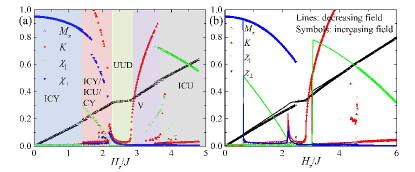
Figure 3: (color online) (a) Magnetic field dependence of different observables for $\mathbf{H}\parallel\hat{z}$ in equilibrium simulation. Due to the nature of the first order phase transition, several phases can coexist in certain magnetic field region. (b) Same as (a) but obtained with sweep of magnetic fields. Here $T=0.02J$ and $M_{z}$ is the total magnetization along the field direction.

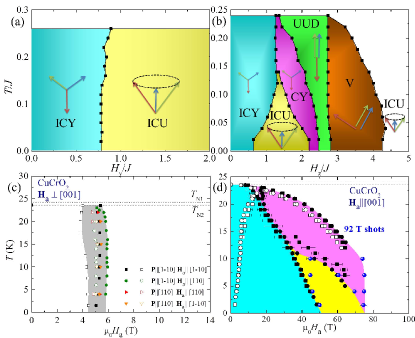
Figure 4: (color online) Calculated phase diagram of ${\cal H}$ when ${\bf H}$ is along the (a) ${\hat{y}}$ and (b) ${\hat{z}}$ directions. The phase boundary is obtained by sweeping $H$ [see Figs. 2 (b) and 3 (b)]. The phase boundaries between ICY, ICU and CY in (b) are obtained by down-sweeps of $H$. Experimental phase diagram for (c) $\mathbf{H}_{a}||\hat{y}$ and (d) $\mathbf{H}_{a}||\hat{z}$ based on Mun et al. (2014). Solid circles and squares are based on ${\bf P}\parallel[110]$ and ${\bf P}\parallel[1\bar{1}0]$ measurements, respectively. Open and closed symbols represent transitions observed in down and upsweeps of $H_{a}$, respectively. New points taken with 92 T shots are shown in blue. Phase transitions are determined from inflection points (positive or negative peaks in $dP/dt$ data), and the error bars indicate the 90% height of the peaks.

The precise location of the strong first-order phase transitions is difficult to determine with MC simulations. Fig. 4(b) shows a rough phase diagram obtained for ${\bf H}\parallel{\hat{z}}$ based on the $H$-dependence of the order parameters at different temperatures. The UUD phase appears at about 100 T for parameters $J=2.3$ meV and $g\approx 2$ relevant to $\mathrm{CuCrO_{2}}$. Poienar et al. (2010) Our simulations produce the qualitative features of the measured phase diagram, Mun et al. (2014) and we can assign the following phases as a function of increasing field: ICY, ICU, CY, and finally UUD. UUD becomes stable roughly at 1/3 of the saturation field. The magnetic states cannot be directly obtained from electric polarization measurements. Mun et al. (2014) Therefore, the proposed states can be checked by other techniques, such as muon spin spectroscopy. We remark that the phase diagram for $\mathrm{CuCrO_{2}}$ is very similar to another TLA compound $\mathrm{Cs_{2}CuCl_{4}}$. Tokiwa et al. (2006)

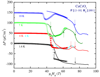
Figure 5: (color online) ${\bf P}$ vs ${\bf H}_{a}$ data measured on the upsweep of a 65 T capacitor-driven magnet (points) Mun et al. (2014) and with shots up to 92 T in the 100 T multi-shot magnet (lines, this work). The variation with $H_{a}$ sweep rate is discussed in the text and the Supplemental Information. SI Arrows indicate phase transitions based on the 92 T data shown as blue points in Fig. 4

In addition to our simulations, we have extend measurements of ${\bf P}({\bf H}_{a})$ to 92 T in the 100 T multi-shot magnet of the NHMFL-PFF in Los Alamos. ${\bf P}||{\hat{y}}$ was measured with ${\bf H}_{a}||{\hat{x}}$ and ${\hat{z}}$ with the same methods and samples as Mun et al. Mun et al. (2014). A poling electric field of 650 kV/m was used. For ${\bf H}_{a}\parallel{\hat{x}}$ we find no additional features in ${\bf P}({\bf H}_{a})$ up to 92 Tesla (not shown), indicating that the cycloidal spiral phase persists beyond that field. The ${\bf P}$ data with ${\bf H}_{a}\parallel{\hat{z}}$ are shown in Fig. 5 for 1.6 K $\leq T\leq$ 10 K and for upsweeps of $H_{a}$. Data in a 65 T magnet from Mun et al. (2014) are shown for comparison. In qualitative agreement with our calculations, we observe significant differences in the width and position of the phase boundaries for different magnetic field sweep rates $dH_{a}/dt$. For example, at the 50 T transition, $dH_{a}/dt$ for a 92 T shot in the 100 T magnet is almost three times higher than for a 65 T shot in the 65 T magnet, and $dH_{a}/dt$ varies with maximum field in a given magnet. Sweep-rate dependences were also previously observed at the 5.3 T spin flop transition for ${\bf H}_{a}\perp{\hat{c}}$. Mun et al. (2014) With that caveat, we determine the transitions in the 92 T $P(H_{a})$ data from peaks in $dP/dt$ Mun et al. (2014), and the error bars from the width of the peaks at 90% of their height. The transitions are indicated as arrows in the $P(H_{a})$ data in Fig. 5 and as blue points in the phase diagram of Fig. 4.

To calculate the precise evolution of ${\bf P}$ within the Arima model hisa Arima (2007), it is necessary to know the position of the O atoms. Without knowing these positions, we still expect that the electric polarization should be similar for the CY and ICY phases because the absolute value of $q$ only changes by a very small amount. In contrast, the intermediate ICU phase (cycloidal spiral) should produce a rather different value of ${\bf P}$ because the magneto-electric coupling has a different origin. Mostovoy (2006) This result is consistent with our measured $H_{a}$-dependence of ${\bf P}$ shown in Fig. 5.

To summarize, we find qualitative agreement between theory and experiment. Our simple 2D model reproduces the incommensurate proper-screw spiral observed in experiments, Soda et al. (2009, 2010) and the phase transition to an incommensurate cycloidal spiral observed for ${\bf H}_{a}\parallel ab$. It also predicts a series of commensurate and incommensurate phases with increasing $H_{z}$, which is in rough agreement with the oscillations observed in the electric polarization. Both calculations and experiments show very strong hysteresis between up and down sweeps. Finally, our results demonstrate how a subtle competition between spatial and spin anisotropy, magnetic frustration and thermal fluctuations can lead to large changes of magneto-electric properties induced by relatively small energy scales.

The authors are grateful to Yoshitomo Kamiya and Gia-Wei Chern for helpful discussions. Computer resources were supported by the Institutional Computing Program in LANL. This work was carried out under the auspices of the NNSA of the U.S. DOE at LANL under Award No. DEAC52-06NA25396, and was supported by the U.S. Department of Energy, Office of BES ”Science at 100 Tesla” program. The NHMFL Pulsed Field Facility is funded by the US National Science Foundation through Cooperative Grant No. DMR-1157490, the State of Florida, and the US Department of Energy. The research leading to these results has also received funding from the European Community’s Seventh Framework Programme (FP7/2007-2013) under Grant Agreement No. 290605 (PSIFELLOW/COFUND).

I Supplementary material

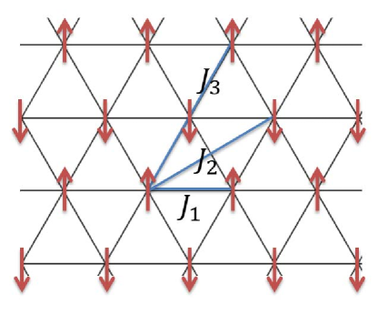
Figure 6: (color online) Schematic view of the collinear spin configuration that is stabilized at $T=0$ and ${\bf H}=0$ for the Hamiltonian parameters of Ref. Frontzek et al., 2011. Here the spins are parallel to the $z$ axis.

II Comparison of the energy for the collinear and proper-screw spiral phase

Our simulations show that the parameters derived in Ref. Frontzek et al., 2011 lead to the collinear spin configuration depicted in Fig. 6 for $T=0$ and ${\bf H}=0$. This result can also be obtained analytically by considering the Hamiltonian used in Ref. Frontzek et al., 2011:

$$\mathcal{H}=\sum_{<ij>}J_{{ij}}\mathbf{S}_{i}\cdot\mathbf{S}_{j}+\sum_{i}\left[\frac{1}{2}A_{x}S_{i,x}^{2}-\frac{1}{2}A_{z}S_{i,z}^{2}-\mathbf{H}\cdot\mathbf{S}_{i}\right],$$ (4)

which include the second and third-neighbor interactions shown in Fig. 6. Here $|S|=1$. Because the $x$ and $z$ directions correspond to the hard and easy-axis, respectively, spins are parallel to the $yz$ plane for the spiral phase and to the $z$-axis for the collinear phase. The weak interlayer coupling is neglected for the moment. For $T=0$ and ${\bf H}=0$, the energy per site of the $120^{\circ}$ proper-screw phase is

$$E_{s}=-\frac{3}{2}J_{1}+3J_{2}-\frac{3}{2}J_{3}-\frac{1}{4}A_{z},$$ (5)

while the energy for the collinear configuration in Fig. 6 is

$$E_{c}=-J_{1}-J_{2}+3J_{3}-\frac{1}{2}A_{z}.$$ (6)

For the Hamiltonian parameters of Ref. Frontzek et al., 2011, $J_{1}=2.8$ meV, $J_{2}=0.48$ meV, $J_{3}=0.08$ meV and $A_{z}=0.96$ meV, we have $E_{s}=-3.12$ meV and $E_{c}=-3.52$ meV. The weak interlayer coupling, $|J_{z}|=0.02$ meV, is clearly not sufficient to stabilize the proper-screw phase. Therefore, the parameters provided by Ref. Frontzek et al., 2011 lead to the collinear spin state depicted in Fig. 6, which is inconsistent with the experimental observations.

III Simulation details

In our simulations, we first anneal the systems from a high temperature to a target temperature using the standard Metropolis algorithm. The MC measurements start after the system reaches equilibrium. Typically we use $5\times 10^{5}$ MC Sweeps (MCS) for annealing, $5\times 10^{5}$ MC Sweeps (MCS) for equilibration, and another $5\times 10^{5}$ MCS for measurements. The typical system size is $L\times L=48\times 48$, but larger sizes of $L=96$ were used to verify the irrelevance of finite size effects.

We have also performed additional simulations by sweeping magnetic fields gradually. In this case, after increasing $H$ by 0.01$J$, we equilibrate the system with $10^{4}$ MCS and perform measurements for another $10^{4}$ MCS.

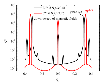
Figure 7: (color online) Spin structure factor ${S}^{zz}(q_{x},q_{y}=0)$ obtained by down-sweep of magnetic fields at $T=0.02J$.

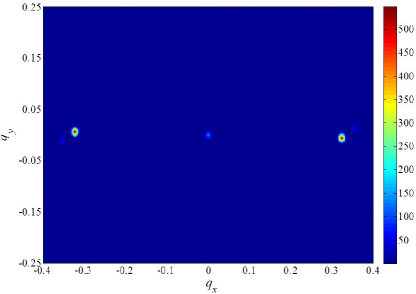
Figure 8: (color online) Spin structure factor ${S}^{zz}(\mathbf{q})$ near the ICY-ICU phase boundary at $T=0.02J$.

IV Spin structure factor

To characterize the transition from the incommensurate Y (ICY) phase to commensurate Y (CY) phase, we have also calculated the spin structure factor

$$S^{\mu\mu}({\bf q})=\frac{1}{N}\sum_{i,j}\exp[{i{\bf q}\cdot{({\bf r}_{i}-{\bf r}_{j})}}]S^{\mu}_{\bf r_{i}}S^{\mu}_{\bf r_{j}},$$ (7)

where $\mu=x,\ y,\ z$. The calculations of ${S}^{zz}(\mathbf{q})$ for the CY and ICY phases obtained by down-sweep of the magnetic fields are shown in Fig. 7. It is clear that the optimal $q$ value deviates from $q=1/3$ for the CY phase to $q=0.3125$ for the ICY phase. ${S}^{zz}(\mathbf{q})$ has a peak at $q=0$ because there is a uniform $S_{z}$ component induced by $H_{z}$. The peak broadening of ${S}^{zz}(\mathbf{q})$ in Fig. 7 is mainly due to finite size effects: $\Delta q=2\pi/N$ (the thermal broadening is much smaller at $T=0.02J$).

Besides the main peak at the optimal $q$, there are additional secondary peaks shown in Fig. 7. These secondary peaks are in general smaller than the main peak by several orders of magnitude. However, the amplitude of the secondary peaks increases and becomes only one order of magnitude smaller than the amplitude of the main peak near the ICY-ICU phase boundary (see Fig. 8). This observation explains the small discrepancy between the transition field derived analytically for single-${\bf q}$ orderings and the value that is obtained from our MC simulations.

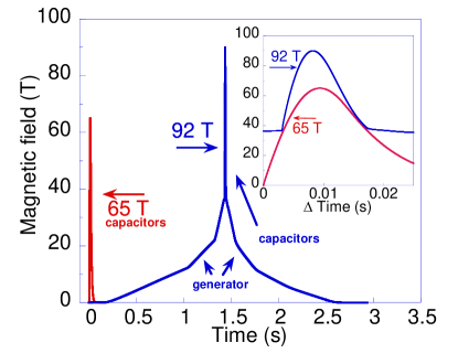
Figure 9: (color online) Magnetic field vs time profile of a 65 T shot in the 65 T capacitor-driven magnet (red), and a 92 T shot in the 100 T generator and capacitor-driven magnet (blue). The inset shows the same data shown zoomed to the high-field capacitor-driven region.

V Experimental details

Figure 9 shows the magnetic field $H_{a}$ versus time $t$ for the 65 T capacitor-driven magnet, and for the 100 T magnet that is driven by a combination of a three-phase generator and a capacitor bank. The slow features are due to the generator, and the sharp spike due to the capacitor bank. At 50 T, $dH_{a}/dt$ is 7.4 T/s for a 65 T pulse in the capacitor-driven 65 T magnet, and $dH_{a}/dt$ is 20 T/s for a 92 T pulse in the capacitor-and-generator-driven 100 T magnet. In the 65 T magnet, $dH_{a}/dt$ at a given field scales with the peak field of the magnetic field pulse. In the 100 T magnet the same relation holds only for the capacitor-driven portion of the pulse.

In our experimental data we can rule out significant sweep-rate dependences created by eddy currents or magnetocaloric heating for the following reasons: 1) with increasing $dH_{a}/dt$, the $\sim 50$ T transition shifts to higher magnetic fields, while with increasing temperature this transition moves to lower magnetic fields. Furthermore, no dramatic differences in transition widths are seen as a function of temperature, and no differences are observed between the $<4$ K data where the sample is cooled by immersion in liquid helium, and the $>4$ K data where the sample is less efficiently cooled by helium gas. On the other hand, the width of the transition changes dramatically with $dH_{a}/dt$.

References

- Kadowaki et al. (1990) H. Kadowaki, H. Kikuchi, and Y. Ajiro, J. Phys.: Conden. Matter 2, 4485 (1990).
- Crottaz et al. (1996) O. Crottaz, F. Kubel, and H. Schmid, Journal of Solid State Chemistry 122, 247 (1996).
- Poienar et al. (2010) M. Poienar, F. Damay, C. Martin, J. Robert, and S. Petit, Phys. Rev. B 81, 104411 (2010).
- Frontzek et al. (2011) M. Frontzek, J. T. Haraldsen, A. Podlesnyak, M. Matsuda, A. D. Christianson, R. S. Fishman, A. S. Sefat, Y. Qiu, J. R. D. Copley, S. Barilo, S. V. Shiryaev, and G. Ehlers, Phys. Rev. B 84, 094448 (2011).
- Vasiliev et al. (2013) A. M. Vasiliev, L. A. Prozorova, L. E. Svistov, V. Tsurkan, V. Dziom, A. Shuvaev, A. Pimenov, and A. Pimenov, Phys. Rev. B 88, 144403 (2013).
- Soda et al. (2009) M. Soda, K. Kimura, T. Kimura, M. Matsuura, and K. Hirota, Journal of the Physical Society of Japan 78, 124703 (2009).
- Soda et al. (2010) M. Soda, K. Kimura, T. Kimura, and K. Hirota, Phys. Rev. B 81, 100406 (2010).
- Kimura et al. (2008) K. Kimura, H. Nakamura, K. Ohgushi, and T. Kimura, Phys. Rev. B 78, 140401 (2008).
- Seki et al. (2008) S. Seki, Y. Onose, and Y. Tokura, Phys. Rev. Lett. 101, 067204 (2008).
- Kimura et al. (2009a) K. Kimura, H. Nakamura, S. Kimura, M. Hagiwara, and T. Kimura, Phys. Rev. Lett. 103, 107201 (2009a).
- Poienar et al. (2009) M. Poienar, F. m. c. Damay, C. Martin, V. Hardy, A. Maignan, and G. André, Phys. Rev. B 79, 014412 (2009).
- Kajimoto et al. (2010) R. Kajimoto, K. Nakajima, S. Ohira-Kawamura, Y. Inamura, K. Kakurai, M. Arai, T. Hokazono, S. Oozono, and T. Okuda, Journal of the Physical Society of Japan 79, 123705 (2010).
- hisa Arima (2007) T. hisa Arima, Journal of the Physical Society of Japan 76, 073702 (2007).
- Kimura et al. (2009b) K. Kimura, T. Otani, H. Nakamura, Y. Wakabayashi, and T. Kimura, Journal of the Physical Society of Japan 78, 113710 (2009b).
- Aktas et al. (2013) O. Aktas, G. Quirion, T. Otani, and T. Kimura, Phys. Rev. B 88, 224104 (2013).
- Ehlers et al. (2013) G. Ehlers, A. A. Podlesnyak, M. Frontzek, R. S. Freitas, L. Ghivelder, J. S. Gardner, S. V. Shiryaev, and S. Barilo, Journal of Physics: Condensed Matter 25, 496009 (2013).
- Fishman (2011) R. S. Fishman, Journal of Physics: Condensed Matter 23, 366002 (2011).
- Mun et al. (2014) E. Mun, M. Frontzek, A. Podlesnyak, G. Ehlers, S. Barilo, S. V. Shiryaev, and V. S. Zapf, Phys. Rev. B 89, 054411 (2014).
- Yamaguchi et al. (2010) H. Yamaguchi, S. Ohtomo, S. Kimura, M. Hagiwara, K. Kimura, T. Kimura, T. Okuda, and K. Kindo, Phys. Rev. B 81, 033104 (2010).
- Frontzek et al. (2012) M. Frontzek, G. Ehlers, A. Podlesnyak, H. Cao, M. Matsuda, O. Zaharko, N. Aliouane, S. Barilo, and S. V. Shiryaev, Journal of Physics: Condensed Matter 24, 016004 (2012).
- Note (1) A similar Hamiltonian with next NN AFM interaction and next-next NN AFM interaction was proposed based on inelastic neutron scattering measurements. Poienar et al. (2010); Frontzek et al. (2011) The parameters derived in Ref. \rev@citealpPoienar10 however lead to a collinear ground state at zero magnetic field, which is inconsistent with experiments (see the supplemental information for details). In Ref. Frontzek et al. (2011), the incommensurate spiral is stabilized by a ferromagnetic interlayer coupling because the layers are not vertically stacked along the -axis. This Hamiltonian was used in Refs. Fishman et al. (2012); Haraldsen et al. (2012); Fishman (2011) for and . It is a subtle issue whether the incommensurability results from the inequivalent intra-layer bonds or/and from the weak frustrated interlayer coupling. Here we seek for a minimal 2D model with only anisotropic NN AFM interactions to qualitatively reproduce our experimental observations. Therefore, in our model, the incommensurability is induced by the anisotropic exchange interaction produced by the lattice distortion that was observed with x-ray diffraction measurements. Kimura et al. (2009b) Because the magnetic ground state ordering is highly sensitive to small perturbations, it is quite natural that our phase diagram differs from those reported in previous Refs. Fishman et al. (2012); Haraldsen et al. (2012); Fishman (2011).
- Miyashita (1986) S. Miyashita, Journal of the Physical Society of Japan 55, 3605 (1986).
- Griset et al. (2011) C. Griset, S. Head, J. Alicea, and O. A. Starykh, Phys. Rev. B 84, 245108 (2011).
- Watarai et al. (2001) S. Watarai, S. Miyashita, and H. Shiba, Journal of the Physical Society of Japan 70, 532 (2001).
- (25) The supplemental information contains comparison of energy between a collinear and the proper-screw spiral phase, simulation details, the spin structure factor, magnetic field pulse profile for the 65 T and 100 T magnets, and a discussion of why magnetocaloric or eddy current effects cannot account for the observed sweep rate dependence.
- Shender (1982) E. F. Shender, Sov. Phys. JETP 56, 178 (1982).
- Henley (1989) C. L. Henley, Phys. Rev. Lett. 62, 2056 (1989).
- Tokiwa et al. (2006) Y. Tokiwa, T. Radu, R. Coldea, H. Wilhelm, Z. Tylczynski, and F. Steglich, Phys. Rev. B 73, 134414 (2006).
- Mostovoy (2006) M. Mostovoy, Phys. Rev. Lett. 96, 067601 (2006).
- Fishman et al. (2012) R. S. Fishman, G. Brown, and J. T. Haraldsen, Phys. Rev. B 85, 020405 (2012).
- Haraldsen et al. (2012) J. T. Haraldsen, R. S. Fishman, and G. Brown, Phys. Rev. B 86, 024412 (2012).