Cosmic ray tests of a GEM-based TPC prototype
operated in Ar-CF₄-isobutane gas mixtures: II

Abstract

The spatial resolution along the pad-row direction was measured with a GEM-based TPC prototype for the future linear collider experiment in order to understand its performance for tracks with finite projected angles with respect to the pad-row normal. The degradation of the resolution due to the angular pad effect was confirmed to be consistent with the prediction of a simple calculation taking into account the cluster-size distribution and the avalanche fluctuation.

1 Introduction

In the previous paper [1] we demonstrated the feasibility of a GEM-based Time Projection Chamber (TPC) operated in an Ar-CF₄-isobutane gas mixture as a central tracker (LCTPC) for the future linear collider experiments (ILC [2] and CLIC [3]). The spatial resolution along the pad-row direction was presented for tracks nearly perpendicular to the pad row in Ref. [1] because the resolution in the $r$-$\phi$ plane better than $\sim$ 100 $\mu$m per pad row for stiff and radial tracks is of prime importance for the physics goals of the experiments. A TPC equipped with GEM readout is certainly an ideal main tracker, which is free from the $E\times B$ and the angular wire effects inherent in conventional TPCs with MWPC readout.

It should be noted, however, that the azimuthal resolution degrades with increasing projected track angle ($\phi$) measured from the pad-row normal because of the angular pad effect as far as conventional pads are employed for readout. As will be seen the angular pad effect adds an almost constant offset to the resolution with its amount depending on the pad height as well as the track angle. Therefore the requirement for the spatial resolution above would not be met for inclined tracks. The degraded resolution for slanted and/or low-momentum tracks provided by the central tracker could affect the physics capability of the whole detector system. An example is the need for good energy resolution for soft jets; thus it is important to understand whether such things can be affected by the design of the TPC.

In this paper the resolutions measured with cosmic rays for inclined tracks in a prototype TPC are presented and compared to the expectation in order to provide a basis for the optimization of the pad height of the LCTPC.

The expected deterioration of the resolution for inclined tracks, compared to that for right angle tracks, is estimated in Section 2. The comparison of the measured resolution with the expectation is presented in Section 3 after a brief description of the experiment. Section 4 is devoted to a discussion and Section 5 concludes the paper.

2 Expectation

For right angle tracks ($\phi=0^{\circ}$) the resolution along the pad-row direction ($\sigma_{\rm X}$) is approximately given by

$$\sigma_{\rm X}^{2}=\sigma_{\rm X00}^{2}+\frac{D^{2}}{n_{\rm eff}}\cdot z$$ (1)

where $\sigma_{\rm X00}$ is the intrinsic resolution, $D$ is the diffusion constant, $n_{\rm eff}$ is the effective number of electrons per pad row, and $z$ is the drift distance [4]. It is worth noting that the value of $n_{\rm eff}$ is almost independent of the drift distance [5]. Even in the case of finite track angle the explicit drift-distance dependence (the second term) of the resolution is scarcely affected by practically small $\phi$ [6]. The first term is, on the other hand, sensitive to the track angle. It may be expressed as

$$\sigma_{\rm X0}^{2}=\sigma_{\rm X00}^{2}+\frac{h^{2}\cdot\tan^{2}\phi}{12\cdot N_{\rm eff}}$$ (2)

where $h$ is the pad height and $N_{\rm eff}$ is the effective number of clusters per pad row (see footnote 3). The second term in Eq. (2) represents the contribution of the angular pad effect to the resolution, which is parametrized by $N_{\rm eff}$.

In fact, $N_{\rm eff}$ is a function of $\phi$, $\theta$, $z$ and $h$:

$$N_{\rm eff}=N_{\rm eff}(\phi,\theta,z,h)$$ (3)

where $\theta$ is the angle between the track and the readout pad plane. Let us consider first the $h$ dependence of $N_{\rm eff}$, i.e. $N_{\rm eff}(0,0,z,h)$. The average number of clusters per pad row ($\left<N\right>$) is proportional to $h$. Furthermore the $z$ dependence of the effective number of clusters due to de-clustering is expected to be small [6]. Accordingly

$$N_{\rm eff}(0,0,z,h)\sim N_{\rm eff}(0,0,0,h)=N_{\rm eff}(\left<N\right>)\;.$$ (4)

For a fixed number of clusters $N$, $N_{\rm eff}$ is given by

$$N_{\rm eff}(N)=\left<\sum_{i=1}^{N}Q_{i}^{2}\;/\left(\sum_{i=1}^{N}Q_{i}\right)^{2}\right>^{-1}$$ (5)

where $Q_{i}$ is the total charge of the cluster $i$ given by

$$Q_{i}=\sum_{j=1}^{n_{i}}q_{j}$$ (6)

with $q_{j}$ being the amplified signal of the $j$-th electron in the cluster $i$ of size $n_{i}$ (see Appendix). $N_{\rm eff}$ was estimated by numerical calculations, taking into account the cluster-size distribution for argon [7], and is shown in Fig. 1, with (filled circles) and without (open circles) the typical avalanche fluctuation (a Polya distribution with $\theta=0.5$) for each electron. The figure tells us that the effective number of clusters is considerably smaller than $N$ because of the large cluster-size fluctuation. Furthermore it is not a linear function of $N$; see Appendix for a qualitative estimation of $N_{\rm eff}$. In real case, $N$ is not a constant and obeys Poisson statistics with the average $\left<N\right>$. The curves in Fig. 1 show the effective number of clusters as a function of $\left<N\right>$.

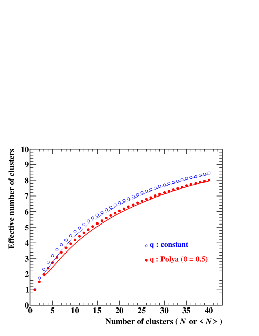
Figure 1: Effective number of clusters ($N_{\rm eff}$) as a function of the total or average number of clusters: plots for fixed $N$, and curves for Poissonly distributed $N$. The filled (open) circles and the full (dotted) curve are calculated with (without) the avalanche fluctuation.

From the curve with the avalanche fluctuation in Fig. 1 the effective number of clusters for a given track angle can be estimated since

$$\left<N\right>=\frac{d\cdot h}{\cos\phi\cdot\cos\theta}$$ (7)

with $d$ being the cluster density ($\sim$ 2.43/mm for minimum ionizing particles in argon [8]), and

$$N_{\rm eff}(\phi,\theta,0,h)=N_{\rm eff}(\left<N\right>)=N_{\rm eff}\left(\frac{d\cdot h}{\cos\phi\cdot\cos\theta}\right)\;.$$ (8)

Let us define $S_{\rm X00}$ as the square root of the second term in Eq. (2) at $z$ = 0:

$$S_{\rm X00}\equiv\frac{h\cdot\tan\phi}{\sqrt{12\cdot N_{\rm eff}(\left<N\right>)}}\;.$$ (9)

Fig. 2 shows $S_{\rm X00}$ as a function of the pad height ($h$) for $\phi$ = 5^∘, 10^∘, 15^∘ and 30^∘, calculated with $\theta$ fixed to 0^∘. It should be noted that the resolutions shown in the figure are the best possible values expected to be obtained without diffusion (at $z$ = 0) and without contribution of the intrinsic term ($\sigma_{\rm X00}$).

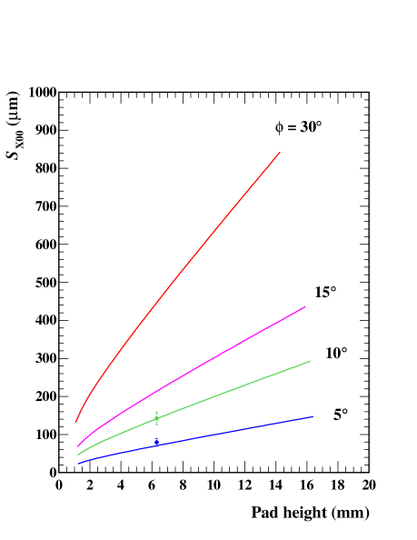
Figure 2: Expected contribution of the angular pad effect ($S_{\rm X00}$) as a function of the pad height ($h$) for different track angles. Poisson statistics is assumed for the number of clusters and a Polya distribution ($\theta=0.5$) is assumed for the avalanche fluctuation. The tracks are assumed to be minimum ionizing and parallel to the readout plane. The points plotted at $h$ = 6.3 mm are the measurements (see Section 3.2).

3 Experiment

3.1 Setup and analysis

We used a small GEM-based TPC prototype (MP-TPC) operated in a gas mixture of Ar (95%)-CF₄ (3%)-isobutane (2%) at atmospheric pressure. The MP-TPC is a small time projection chamber with a maximum drift length of 257 mm. Its gas amplification device is a triple GEM, 100 mm $\times$ 100 mm in size. The amplified electrons are collected by a readout plane placed right behind the GEM stack, having 16 pad rows at a pitch ($h$) of 6.3 mm, each consisting of 1.17 mm $\times$ 6 mm rectangular pads arranged at a pitch of 1.27 mm. The neighboring pad rows are staggered by half a pad pitch. The pad signals are then fed to readout electronics, a combination of preamplifiers, shaper amplifiers and digitizers. See Ref. [1] for details of the experimental setup and the analysis procedure for the cosmic ray tests of the MP-TPC.

We re-analyzed the data taken for the previous paper on the normal incident tracks [1] with different cuts on the track angles. Among the data sets the data collected with a drift field of 250 V/cm and $B$ = 0 T were selected because of its highest statistics and the negligible influence of the finite pad-pitch term in the absence of axial magnetic field [1]. The offset to the resolution due to finite track angle is to be added quadratically as well in the presence of a magnetic field, depending on the local track angle, at drift distances where the finite pad-pitch term is negligible.

The track angle distributions are shown in Fig. 3. As mentioned in Introduction our primary concern in the cosmic ray tests with the MP-TPC was the resolution for right angle tracks. Therefore the acceptance to inclined tracks was limited by trigger-counter arrangement in order to reduce the trigger rate to the relatively slow readout electronics. The maximum available track angle is thus $|\phi|\hbox{ \raise 3.0pt\hbox to0.0pt{$<$}\raise-3.0pt\hbox{$\sim$} }10^{\circ}$ as seen in Fig. 3 (a).

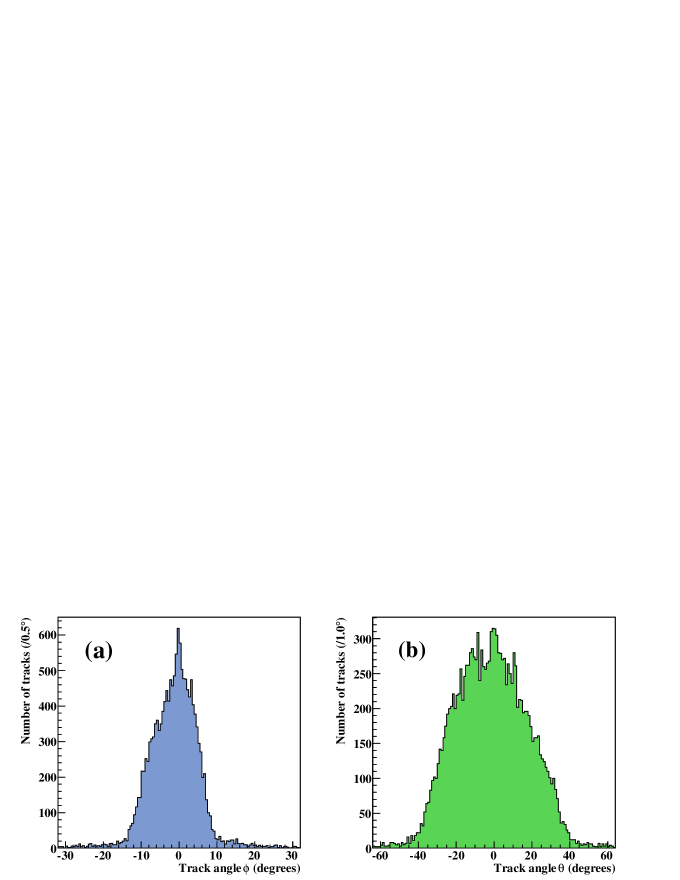
Figure 3: Track angle distributions: (a) for $\phi$, and (b) for $\theta$.

3.2 Results

The spatial resolutions along the pad-row direction are shown in Fig. 4 for $|\phi|$ = 0^∘, 5^∘ and 10^∘, for tracks nearly parallel ($|\theta|\leqq 10^{\circ}$) to the readout plane. The azimuthal angle cuts are the nominal values $\pm$ 2^∘. The resolutions squared as function of the drift distance ($z$) were fitted by a function $\sigma_{\rm X}^{2}=\sigma_{\rm X0}^{2}+D^{2}/n_{\rm eff}\cdot z$ for free parameters $\sigma_{\rm X0}$ and $n_{\rm eff}$, with the value of $D$ fixed to 315 $\mu$m/$\sqrt{\rm cm}$ given by Magboltz [9]. $S_{\rm X00}$ and $N_{\rm eff}$ were then obtained using Eqs. (2) and (9) for each $\phi$, assuming $\sigma_{\rm X00}$ to be $\sigma_{\rm X0}$ measured for $\phi$ = 0^∘. The resultant $\sigma_{\rm X0}$, $n_{\rm eff}$, $S_{\rm X00}$ and $N_{\rm eff}$ are summarized in Table 1 along with the values of $S_{\rm X00}$ and $N_{\rm eff}$ calculated for $h$ = 6.3 mm. The measured values of $S_{\rm X00}$ are plotted also in Fig. 2.

The measured values of $S_{\rm X00}$ and $N_{\rm eff}$ are consistent with those given by the calculation. In addition, the values of $n_{\rm eff}$ for inclined tracks are close to that for normal incident tracks as expected and are consistent with an estimation in Ref. [4].

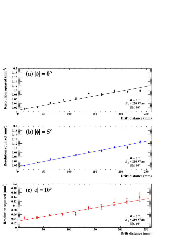
Figure 4: Resolution squared ($\sigma_{\rm X}^{2}$) as a function of the drift distance ($z$): (a) for $|\phi|$ = 0^∘, (b) for $|\phi|$ = 5^∘ and (c) for $|\phi|$ = 10^∘. See text for the straight lines fitted through the data points.

Table 1: Results of measurement and calculation

	$\sigma_{\rm X0}$ ($\mu$m)	$n_{\rm eff}$	$S_{\rm X00}$ ($\mu$m)		$N_{\rm eff}$
$\phi$ (∘)	Measured	Measured	Measured	Calculated	Measured	Calculated
0	96 $\pm$   6	22.8 $\pm$ 0.8	$\equiv$ 0	0	$-$	5.11
5	124 $\pm$   5	21.5 $\pm$ 0.7	79.2 $\pm$ 10.2	70.3	4.0 $\pm$ 1.1	5.12
10	171 $\pm$ 14	24.5 $\pm$ 2.7	142.1 $\pm$ 16.3	141.2	5.1 $\pm$ 1.2	5.15

4 Discussion

The figure of merit for the azimuthal spatial resolution of a cylindrical TPC is the resolution per projected track length in the $r$-$\phi$ plane along the radial direction. From Eqs. (1), (2) and (9), the resolution per pad row is expressed as

$$\sigma_{\rm X}^{2}\sim\sigma_{\rm X00}^{2}+S_{\rm X00}^{2}+\frac{D^{2}}{n_{\rm eff}}\cdot z$$ (10)

at drift distances where the finite pad-pitch term is negligible, and each of the three terms is a function of the pad height $h$.

We consider here the effect of splitting a pad row with $h$ = $H$ into a couple of identical pad rows with a height of $H$/2. Let us assume for simplicity that the combined track coordinate is given by the average of the two measurements provided by the neighboring pad rows with $h$ = $H$/2. Then the resolution per projected track length $H$ becomes

$$\sigma_{\rm X}^{2}=\frac{{\sigma_{\rm X}^{\ast}}^{2}}{2}$$ (11)

where $\sigma_{\rm X}^{\ast}$ is the resolution obtained with a single pad row with the halved height. The diffusion contribution (the third term in Eq.(10)) is almost unaffected since $n_{\rm eff}$ is approximately proportional to the pad height [5].

On the other hand, the angular pad effect ($S_{\rm X00}$) is reduced appreciably. We temporarily assume $N_{\rm eff}(\left<N\right>)$ to be proportional to the pad height. Then

$$S_{\rm X00}^{2}\propto h$$ (12)

from Eq. (9), and the combined contribution of the angular pad effect ($S_{\rm X00}$) per projected track length $H$ is halved because of Eq. (11). Actually $S_{\rm X00}$ is reduced by more than a factor of 2 because Eq. (12) gives an overestimate for a smaller $h$ (see Fig. 2).

In addition, $\sigma_{\rm X00}^{2}$ at long drift distances can be shown mathematically to be

$$\sigma_{\rm X00}^{2}=\frac{B_{0}^{2}}{n_{\rm eff}}$$ (13)

with a constant $B_{0}$ independent of the pad height if the contribution of the electronic noise is negligible (see Appendix B of Ref. [1]). Similarly to the diffusion contribution, the intrinsic term ($\sigma_{\rm X00}$) in the combined resolution is expected to be close to the counterpart in the resolution for a single pad row with $h$ = $H$.

Consequently the net effect of halving the pad height on the resolution per projected track length is essentially the alleviation of the angular pad effect ($S_{\rm X00}$) by more than a factor of 2. For example, Eq. (9) gives $S_{\rm X00}$ $\sim$ 140 $\mu$m (450 $\mu$m) for $\phi$ = 10^∘ (30^∘) with $h$ = 6.3 mm, while the corresponding value for a couple of pad rows with $h$ = 3.15 mm is about 60 $\mu$m (200 $\mu$m). The spatial resolutions, and therefore the momentum resolutions improve significantly for slanted and/or low momentum tracks with the shorter pads.

The number of voxels in the sensitive volume of a TPC is doubled if the pad height is halved (with the electronics channel density doubled). This would enhance the pattern recognition capability and the d$E$/dx resolution of the TPC as well.

5 Conclusion

The azimuthal spatial resolutions for inclined tracks were measured with a GEM-equipped prototype TPC as well as for right angle tracks. The angular pad effect contributes as a virtually constant offset to the spatial resolution to be added quadratically, depending on the track angle and the pad height. The offsets are found to be consistent with the predictions given by a simple model calculation taking into account the cluster-size distribution and the avalanche fluctuation.

The results are expected to be useful in optimizing the pad height of the LCTPC from the physics point of view.

Appendix A Behavior of $N_{\rm eff}(N)$

The effective number of clusters ($N_{\rm eff}$) parametrizes the degradation of the resolution due to the angular pad effect (the second term in Eq. (2)). We consider here the behavior of $N_{\rm eff}$ at $z=0$ as a function of the fixed total number of clusters per pad row ($N$), qualitatively for $N$ = 1, 2, 4 and $\infty$. The track coordinate ($X$) along the pad-row direction is assumed to be determined from the charge centroid of the clusters detected by the pad row having an infinitesimal pad pitch. The clusters are fully intact at $z=0$ and are assumed to be point-like.

In order to estimate $N_{\rm eff}(N)$ it is necessary to evaluate the variance ($\equiv{S_{N}}^{2}$) of the charge centroid of $N$ clusters, each with charge $Q_{i}$ and coordinate $x_{i}$, which are randomly scattered over the lateral range on the pad row covered by an inclined track ($h\cdot\tan\phi$).

1. $N=1$
   The resolution ($\equiv S_{1}$) does not depend on the cluster charge ($Q$).

   $${S_{1}}^{2} = \frac{h^{2}\cdot\tan^{2}\phi}{12}\;,\;\;{\rm and}$$ (14)

   $$N_{\rm eff}(1) = 1\;\;\;{\rm by\;\;definition}.$$ (15)

2. $N=2$
   Let the coordinates and charges of the clusters be $(x_{1},Q_{1})$ and $(x_{2},Q_{2})$. Their weighted-mean coordinate is given by

   $$X=\frac{x_{1}Q_{1}+x_{2}Q_{2}}{Q_{1}+Q_{2}}\;.$$ (16)

   Its variance (${S_{2}}^{2}$) is given by

   $${S_{2}}^{2} \equiv \left<(X-\left<X\right>)^{2}\right>$$ (17)

   $$= \left<\left(\frac{(x_{1}-\left<X\right>)\cdot Q_{1}+(x_{2}-\left<X\right>)\cdot Q_{2}}{Q_{1}+Q_{2}}\right)^{2}\right>$$

   $$= \left<\frac{(x_{1}-\left<X\right>)^{2}\cdot{Q_{1}}^{2}+(x_{2}-\left<X\right>)^{2}\cdot{Q_{2}}^{2}}{(Q_{1}+Q_{2})^{2}}\right>$$

   $$= \left<(x-\left<x\right>)^{2}\right>\cdot\left<\frac{{Q_{1}}^{2}+{Q_{2}}^{2}}{(Q_{1}+Q_{2})^{2}}\right>$$

   $$= {S_{1}}^{2}\cdot\left<\frac{(Q_{1}+Q_{2})^{2}-2Q_{1}Q_{2}}{(Q_{1}+Q_{2})^{2}}\right>$$

   $$= {S_{1}}^{2}\cdot\left(1-2\cdot\left<\frac{Q_{1}Q_{2}}{(Q_{1}+Q_{2})^{2}}\right>\right)$$

   $$\geqq {S_{1}}^{2}\;/2\;.$$

   The third and fourth lines in the equation above are justified since the variables $x$ and $Q$ are not correlated, whereas the last line follows from

   $$Q_{1}Q_{2}\;/(Q_{1}+Q_{2})^{2} \leqq 1/4$$ (18)

   $$\because\;(Q_{1}-Q_{2})^{2} = (Q_{1}+Q_{2})^{2}-4Q_{1}Q_{2}\geqq 0\;.$$

   The equality in Eq. (18) holds only when $Q_{1}=Q_{2}$. Therefore, in a general case addressed here

   $$N_{\rm eff}(2)\equiv{S_{1}}^{2}\;/{S_{2}}^{2}<2\;.$$ (19)

3. $N=4$
   

   $$X = \frac{x_{1}Q_{1}+x_{2}Q_{2}+x_{3}Q_{3}+x_{4}Q_{4}}{Q_{1}+Q_{2}+Q_{3}+Q_{4}}$$ (20)

   $$= \frac{x_{1}^{\prime}Q_{1}^{\prime}+x_{2}^{\prime}Q_{2}^{\prime}}{Q_{1}^{\prime}+Q_{2}^{\prime}}$$

   where

   $$x_{1}^{\prime}Q_{1}^{\prime} \equiv x_{1}Q_{1}+x_{2}Q_{2}$$

   $$x_{2}^{\prime}Q_{2}^{\prime} \equiv x_{3}Q_{3}+x_{4}Q_{4}$$

   with $Q_{1}^{\prime}\equiv Q_{1}+Q_{2}$ and $Q_{2}^{\prime}\equiv Q_{3}+Q_{4}$.

   $${S_{4}}^{2} \equiv \left<(X-\left<X\right>)^{2}\right>$$ (21)

   $$= \left<(x^{\prime}-\left<x\right>)^{2}\right>\cdot\left<\frac{{Q_{1}^{\prime}}^{2}+{Q_{2}^{\prime}}^{2}}{(Q_{1}^{\prime}+Q_{2}^{\prime})^{2}}\right>$$

   $$= \left<(x^{\prime}-\left<x\right>)^{2}\right>\cdot\left(1-2\cdot\left<\frac{Q_{1}^{\prime}Q_{2}^{\prime}}{(Q_{1}^{\prime}+Q_{2}^{\prime})^{2}}\right>\right)$$

   $$> {S_{2}}^{2}/2\;,\;\;{\rm with}\;\;{S_{2}}^{2}\equiv\left<(x^{\prime}-\left<x\right>)^{2}\right>\;.$$

   Therefore

   $$\frac{{S_{2}}^{2}}{{S_{4}}^{2}} < 2\;,\;\;{\rm and}$$ (22)

   $$N_{\rm eff}(4) < 2N_{\rm eff}(2)\;.$$ (23)

   Consequently

   $$N_{\rm eff}(1)=1,\;N_{\rm eff}(2)<2,\;N_{\rm eff}(4)<2N_{\rm eff}(2),\;\;{\rm and\;so\;on.}$$ (24)

   Thus $N_{\rm eff}(N)/N$ is expected to be a decreasing function of $N$.

4. $N=\infty$

   $$X = \frac{\sum_{i=1}^{N}x_{i}Q_{i}}{\sum_{i=1}^{N}Q_{i}}$$ (25)

   $${S_{\rm N}}^{2} \equiv \left<(X-\left<X\right>)^{2}\right>$$ (26)

   $$= \left<(x-\left<x\right>)^{2}\right>\cdot\left<\frac{\sum_{i=1}^{N}{Q_{i}}^{2}}{\left(\sum_{i=1}^{N}Q_{i}\right)^{2}}\right>$$

   $$\sim {S_{1}}^{2}\cdot\frac{\left<\sum_{i=1}^{N}{Q_{i}}^{2}\right>}{N^{2}\left<Q\right>^{2}}$$

   $$\sim {S_{1}}^{2}\cdot\frac{1}{N}\cdot\frac{\left<Q^{2}\right>}{\left<Q\right>^{2}}$$

   $$\sim {S_{1}}^{2}\cdot\frac{1}{N}\cdot\frac{\left<Q\right>^{2}+{\sigma_{Q}}^{2}}{\left<Q\right>^{2}}$$

   $$\sim {S_{1}}^{2}\cdot\frac{1}{N}\cdot(1+F^{\prime})$$

   where the relative variance $F^{\prime}\equiv{\sigma_{Q}}^{2}\;/\left<Q\right>^{2}$ with $\sigma_{Q}$ being the standard deviation of the cluster charge, including the fluctuations in cluster size, and in avalanche gain for each electron in the cluster. Actually

   $$F^{\prime}=F+\frac{1}{\left<n\right>}\cdot f$$ (27)

   with $F$ ($f$) being the relative variance of the cluster-size (avalanche-size) fluctuation and $\left<n\right>$ the average cluster size. Therefore

   $$\lim_{N\rightarrow\infty}\frac{N_{\rm eff}(N)}{N}=\frac{1}{1+F^{\prime}}\sim\frac{1}{1+F}$$ (28)

   because $F$ ($\sim$ 2000 for argon [5]) is much greater than $f$ ($\sim$ 1).

References

-
[1]
M. Kobayashi, et al.,
Nuclear Instrumentation and Methods in Physics Research
A 641 (2011) 37. -
[2]
The International Linear Collider,
ILC Technical Design Report, available at
https://www.linearcollider.org/ILC/Publications/Technical-Design-Report. -
[3]
The Compact Linear Collider, Compact Linear Collider,
available at
http://clic-study.org/. -
[4]
Makoto Kobayashi,
Nuclear Instrumentation and Methods in Physics Research
A 562 (2006) 136. -
[5]
Makoto Kobayashi,
Nuclear Instrumentation and Methods in Physics Research
A 729 (2013) 273. - [6] R. Yonamine, et al., Journal of Instrumentation 9 (2014) C03002.
-
[7]
H. Fischle, J. Heintze, B. Schmidt,
Nuclear Instrumentation and Methods in Physics Research
A 301 (1991) 202. -
[8]
A. Sharma, F. Sauli,
Nuclear Instrumentation and Methods in Physics Research
A 350 (1994) 470. -
[9]
S.F. Biagi,
Nuclear Instrumentation and Methods in Physics Research
A 421 (1999) 234.