Kernel-Based Adaptive Online Reconstruction of Coverage Maps With Side Information

Abstract

In this paper, we address the problem of reconstructing coverage maps from path-loss measurements in cellular networks. We propose and evaluate two kernel-based adaptive online algorithms as an alternative to typical offline methods. The proposed algorithms are application-tailored extensions of powerful iterative methods such as the adaptive projected subgradient method and a state-of-the-art adaptive multikernel method. Assuming that the moving trajectories of users are available, it is shown how side information can be incorporated in the algorithms to improve their convergence performance and the quality of the estimation. The complexity is significantly reduced by imposing sparsity-awareness in the sense that the algorithms exploit the compressibility of the measurement data to reduce the amount of data which is saved and processed. Finally, we present extensive simulations based on realistic data to show that our algorithms provide fast, robust estimates of coverage maps in real-world scenarios. Envisioned applications include path-loss prediction along trajectories of mobile users as a building block for anticipatory buffering or traffic offloading.

I Introduction

A reliable and accurate path-loss estimation and prediction, e.g., for the reconstruction of coverage maps, have attracted a great deal of attention from both academia and industry; in fact the problem is considered as one of the main challenges in the design of radio networks [1][2]. A reliable reconstruction of current and future coverage maps will enable future networks to better utilize scarce wireless resources and to improve the quality-of-service (QoS) experienced by the users. Reconstructing coverage maps is of particular importance in the context of (network-assisted) device-to-device (D2D) communication where no or only partial measurements are available for D2D channels [3]. In this case, some channel state information must be extracted or reconstructed from other measurements available in the network and provided to the D2D devices for a reliable decision making process. Another interesting concept where path-loss prediction is expected to play a crucial role is proactive resource allocation [4][5]. Here, the decisions on resource allocation are based not only on present channel state information, but also on information about future propagation conditions. In particular, the quality of service experienced by mobile users can be significantly enhanced if the information about future path-loss propagation conditions along the users’ routes is utilized for proactive resource allocation. Possible applications of proactive resource allocation are:

1. Anticipatory buffering: Assure smooth media streaming by filling the playout buffer before a mobile user reaches a poorly covered area.

2. Anticipatory handover: Avoid handover failures by including a coverage map in the decision-making process.

3. Anticipatory traffic offloading: Reduce cellular traffic load by postponing transmission of a user until it has reached an area covered by WLAN.

In this paper, we consider an arbitrary cellular network, and we address the problem of estimating a two-dimensional map of path-loss values at a large time scale. The path-loss estimation is the key ingredient in the reconstruction of coverage maps, which provides a basis for the development of the proactive resource allocation schemes mentioned above. We propose novel kernel-based adaptive online methods by tailoring powerful approaches from machine learning to the application needs. In the proposed schemes, each base station maintains a prediction of the path-loss in its respective area of coverage. This prediction process is carried out as follows. We assume that each base station in the network has access to measurements that are periodically generated by users in the network. Whenever a new measurement arrives, the corresponding base station updates its current approximation of the unknown path-loss function in its cell. To make this update quickly available to online adaptation function in the network, coverage map reconstruction needs to be an online function itself. Thus, we need to consider machine learning methods that provide online adaptivity at low complexity. The requirement of low complexity is particularly important because measurements arrive continuously, and they have to be processed in real time. The online nature of the algorithm in turn ensures that measurements are taken into account immediately after their arrivals to continuously improve the prediction and estimation quality. In addition, we exploit side information to further enhance the quality of the prediction. By side information, we understand any information in addition to concrete measurements at specific locations. In this paper, we exploit knowledge about the user’s trajectories, and we show how this information can be incorporated in the algorithm. Measurements used as input to the learning algorithm can be erroneous due to various causes. One source of errors results from the fact that wireless users are usually able to determine their positions only up to a certain accuracy. On top of this, the measured values themselves can also be erroneous. Another problem is that users performing the measurements are not uniformly distributed throughout the area of interest and their positions cannot be controlled by the network. This leads to a non-uniform random sampling, and as a results, data availability may vary significantly among different areas. To handle such situations, we exploit side information to perform robust prediction for areas where no or only few measurements are available.

Our overall objective is to design an adaptive algorithm that, despite the lack of measurements in some areas, has high estimation accuracy under real-time constraints and practical impairments. Kernel-based methods are promising tools in this aspect due to their amenability to adaptive and low-complexity implementation [6]. This paper shows how to enhance such methods so that they can provide accurate coverage maps. In particular, we design sparsity-aware kernel-based adaptive algorithms that are able to incorporate side information.

To demonstrate the advantages of the proposed approaches, we present extensive simulations for two scenarios. First, we confine our attention to an urban scenario closely related to practical situations; the scenario is based on realistic path-loss data and realistic emulation of user mobility. Second, we consider a campus network with publicly available real measurement traces at a fairly high spatial resolution.

I-A Contribution Summary

In short, the main contributions of our work are:

1. We demonstrate how kernel-based methods can be used for adaptive online learning of path-loss maps based on measurements from users in a cellular network.

2. We compare state-of-the-art methods with single and multiple kernels with respect to their accuracy and convergence for estimating coverage maps.

3. We show how side information can be incorporated in the algorithms to improve their accuracy in a given time period.

4. We show how to enhance the algorithms by using an iterative weighting scheme in the underlying cost function.

I-B Related Work

Accurately predicting path-loss in wireless networks is an ongoing challenge [1]. Researchers have proposed many different path-loss models in various types of networks, and there are also approaches to estimate the path-loss from measurements [1]. In [7], wireless network measurements are used to evaluate the performance of a large number of empirical path-loss models proposed over the last decades. The authors demonstrate that even the best models still produce significant errors when compared to actual measurements. Regarding measurement-based learning approaches, so far mainly Support Vector Machines (SVM) [8] or Artificial Neural Networks (ANN) [9, 8] have been employed. Aside from that, Gaussian processes [2] and kriging based techniques [10] have recently been successfully used for the estimation of radio maps. In [11], kriging based techniques have been applied to track channel gain maps in a given geographical area. The proposed kriged Kalman filtering algorithm allows to capture both spatial and temporal correlations. However, all these studies use batch schemes; i.e., all (spatial) data needs to be available before applying the prediction schemes. Somehow in between learning and modeling is the low-overhead active-measurement based approach of [12], which aims at identifying coverage holes in wireless networks. The authors use an a-priori model that is fitted based on terrain properties and corrections obtained by measurements, and they evaluate their method in real-world WIFI networks (Google WiFi and the Center for Technology for All Wireless (TFA) at Rice University). In more detail, in a first phase the path-loss characteristics are learned for each terrain/building type and subsequently used to update corresponding parameters in the path-loss model. A second phase involves iterative refinement based on measurements close to the coverage boundary. Although [12] uses measurements to refine iteratively the current path-loss model in an online fashion, to the best of the authors’ knowledge, this paper is the first study to propose online estimation mechanisms for path-loss maps using kernel-based methods. Using such methods, we aim at developing algorithms that can be readily deployed in arbitrary scenarios, without the need of initial tailoring to the environment. In [1, Section VI] the authors expect “general machine learning approaches, and active learning strategies” to be fruitful; however, “applying those methods to the domain of path loss modeling and coverage mapping is currently unexplored.”

In this study we rely on methods such as the Adaptive Projected Subgradient Method (APSM), which is a recently developed tool for iteratively minimizing a sequence of convex cost functions [13]. It generalizes Polyak’s projected subgradient algorithm [14] to the case of time-varying functions, and it can be easily combined with kernel-based tools from machine learning [13][6]. APSM generalizes well-known algorithms such as the affine projection algorithm (APA) or normalized least mean squares (NLMS) [15]. APSM was successfully applied to a variety of different problems, for example, channel equalization, diffusion networks, peak-to-average power ratio (PAPR) reduction, super resolution image recovery, and nonlinear beamforming [6].

I-C Notation

Let $\mathbb{R}$ and $\mathbb{Z}$ denote the sets of real numbers and integer numbers, respectively. We denote vectors by bold face lower case letters and matrices by bold face upper case letters. Thereby $[\bm{x}]_{i}$ stands for the $i$th element of vector $\bm{x}$, and $[\bm{A}]_{i,j}$ stands for the element in the $i$th row and $j$th column of matrix $\bm{A}$. An inner product between two matrices $\bm{A},\bm{B}\in\mathbb{R}^{l\times m}$ is defined by $\langle\bm{A},\bm{B}\rangle:=\mathrm{tr}(\bm{A}^{T}\bm{B})$ where $(\cdot)^{T}$ denotes the transpose operation and $\mathrm{tr}(\cdot)$ denotes the trace. The Frobenius norm of a matrix $\bm{A}$ is denoted by $\lVert\bm{A}\rVert=\langle\bm{A},\bm{A}\rangle^{\frac{1}{2}}$, which is the norm induced by the inner product given above. By $\mathcal{H}$ we denote a (possibly infinite dimensional) real Hilbert space with an inner product given by $\langle\cdot,\cdot\rangle$ and an induced norm $\lVert\cdot\rVert=\langle\cdot,\cdot\rangle^{\frac{1}{2}}$. Note that in this paper we consider different Hilbert spaces (namely of matrices, vectors, and functions) but for notational convenience we use the same notation for their corresponding inner products and induced norms. (The respective Hilbert space will be then obvious from the context.) A set $C\subset\mathcal{H}$ is called convex if $\lambda\bm{y}_{1}+(1-\lambda)\bm{y}_{2}\in C$ $\forall\bm{y}_{1},\bm{y}_{2}\in C,\;\forall\lambda\in(0,1)$. We use $d(\bm{x},C)$ to denote the Euclidean distance of a point $\bm{x}\in\mathcal{H}$ to a closed convex set $C$, which is given by

$$d(\bm{x},C):=\inf\{\lVert\bm{x}-\bm{y}\rVert:\bm{y}\in C\}.$$

Note that the infimum is achieved by some $\bm{y}\in C$ because we are dealing with closed convex sets in a Hilbert space.

I-D Definitions

The projection of $\bm{x}$ onto a nonempty closed convex set $C$, denoted by $P_{C}(\bm{x})\in C$, is the uniquely existing point in the set $\mathrm{argmin}_{\bm{y}\in C}\lVert\bm{x}-\bm{y}\rVert$. Later, if $\mathrm{argmin}_{\bm{y}\in C}\lVert\bm{x}-\bm{y}\rVert$ is a singleton, the same notation is also used to denote the unique element of the set. A Hilbert space $\mathcal{H}$ is called a reproducing kernel Hilbert space (RKHS) if there exists a (kernel) function $\kappa:\mathbb{R}^{m}\times\mathbb{R}^{m}\rightarrow\mathbb{R}$ for which the following properties hold [16]:

1. $\forall\bm{x}\in\mathbb{R}^{m}$, the function $\kappa(\bm{x},\cdot):\mathbb{R}^{m}\rightarrow\mathbb{R}$ belongs to $\mathcal{H}$, and

2. $\forall\bm{x}\in\mathbb{R}^{m}$, $\forall f\in\mathcal{H}$, $f(\bm{x})=\langle f,\kappa(\bm{x},\cdot)\rangle$,

where 2) is called the reproducing property. Calculations of inner products in a RKHS can be carried out by using the so-called “kernel trick”:

$$\langle\kappa(\bm{x}_{i},\cdot),\kappa(\bm{x}_{j},\cdot)\rangle=\kappa(\bm{x_{i}},\bm{x_{j}}).$$

Thanks to this relation, inner products in the high (or infinite) dimensional feature space can be calculated by simple evaluations of the kernel function in the original parameter space.

The proximity operator $\mathrm{prox}_{\gamma f}:\mathcal{H}\rightarrow\mathcal{H}$ of a scaled function $\gamma f$, with $\gamma>0$ and a continuous convex function $f:\mathcal{H}\rightarrow\mathbb{R}$, is defined as

$$\mathrm{prox}_{\gamma f}(\bm{x})=\mathrm{argmin}_{\bm{y}}\left(f(\bm{y})+\frac{1}{2\gamma}\lVert\bm{x}-\bm{y}\rVert^{2}\right).$$

Proximity operators have a number of properties that are particularly suited for the design of iterative algorithms. In particular, the proximity operator is firmly nonexpansive [17], i.e. $(\forall\bm{x},\bm{y}\in\mathcal{H})$

$$\lVert\mathrm{prox}_{f}\bm{x}-\mathrm{prox}_{f}\bm{y}\rVert^{2}+\lVert(\bm{x}-\mathrm{prox}_{f}\bm{x})-(\bm{y}-\mathrm{prox}_{f}\bm{y})\rVert^{2}\leq\lVert\bm{x}-\bm{y}\rVert^{2}$$ (1)

and its fixed point set is the set of minimizers of $f$.

I-E Organization

The paper is organized as follows. In Section II we specify the system model and the path-loss estimation problem. In Section III we outline important mathematical concepts and the basics of the employed kernel-based methods. Moreover we present our modifications to the basic algorithms to incorporate side information and to improve sparsity. In Section IV we numerically demonstrate the performance of the algorithms in realistic urban and campus network scenarios.

II Problem Statement

We now formally state the problem we address in this study. We pose the problem of reconstructing path-loss maps from measurements as a regression problem, and we use the users’ locations as input to the regression task. This is mainly motivated by the increasing availability of such data in modern wireless networks due to the wide-spread availability of low-cost GPS devices. Moreover, path-loss is a physical property that is predominantly determined by the locations of transmitters and receivers. However, the methods we propose are general enough to be used with arbitrary available input. In addition, our methods permit the inclusion of further information as side information. We exemplify this fact in Section III-B, where we incorporate knowledge about the users’ trajectories.

To avoid technical digressions and notational clutter, we consider that all variables in Sections II and III are deterministic. Later in Section IV we drop this assumption to give numerical evidence that the proposed algorithms have good performance also in a statistical sense.

We assume that a mobile operator observes a sequence $\left\{\left(\tilde{\bm{x}}_{n},y_{n}\right)\right\}_{n\in\mathbb{N}}\subset\mathbb{R}^{2}\times\mathbb{R}$, where $\tilde{\bm{x}}_{n}:=\bm{x}_{n}+\bm{\varepsilon}_{x}\in\mathbb{R}^{2}$ is an estimate of a coordinate $\bm{x}_{n}\in\mathbb{R}^{2}$ of the field, $\bm{\varepsilon}_{x}\in\mathbb{R}^{2}$ is an estimation error, and $y_{n}\in\mathbb{R}$ is a noisy path-loss measurement at coordinate $\bm{x}_{n}$ with respect to a particular base station (e.g., the base station with strongest received signal), all for the $n$th measurement reported by an user in the system. The relation between the path-loss measurement $y_{n}$ and the coordinate $\bm{x}_{n}\in\mathbb{R}^{2}$ is given by

$$y_{n}:=f({\bm{x}}_{n})+\varepsilon_{y},$$ (2)

where $f:\mathbb{R}^{2}\to\mathbb{R}$ is an unknown function and $\varepsilon_{y}\in\mathbb{R}$ is an error in the measurement of the path-loss. Measurements $\left(\tilde{\bm{x}}_{n},y_{n}\right)$ arrive sequentially, and they are reported by possibly multiple users in the network. As a result, at any given time, operators have knowledge of only a finite number of terms of the sequence $\left\{\left(\tilde{\bm{x}}_{n},y_{n}\right)\right\}_{n\in\mathbb{N}}$, and this number increases quickly over time.

The objective of the proposed algorithms is to estimate the function $f$ in an online fashion and with low computational complexity. By online, we mean that the algorithms should keep improving the estimate of the function $f$ as measurements $\left(\tilde{\bm{x}}_{n},y_{n}\right)$ arrive, ideally with updates that can be easily implemented.

In particular, in this study we investigate two algorithms having the above highly desirable characteristics. The first algorithm is based on the adaptive projected subgradient method for machine learning [6, 18] (Section III-A), and the second algorithm is based on the more recent multikernel learning technique [19] (Section III-C). The choice of these particular algorithms are motivated by the fact that they are able to cope with large scale problems where the number of measurements arriving to operators is so large that conventional learning techniques cease to be feasible because of memory and computational limitations. Note that, from a practical perspective, typical online learning algorithms need to solve an optimization problem where the number of optimization variables grows together with the number of measurements $\left(\tilde{\bm{x}}_{n},y_{n}\right)$. The algorithms developed in this study operate by keeping only the most relevant data (i. e., the most relevant terms of the sequence $\left\{\left(\tilde{\bm{x}}_{n},y_{n}\right)\right\}_{n\in\mathbb{N}}$) in a set called dictionary and by improving the estimate of the function $f$ by computing simple projections onto closed convex sets, proximal operators, or gradients of smooth functions. We note that the notion of relevance depends on the specific technique used to construct the dictionary, and, for notational convenience, we denote the dictionary index set at time $n$ as

$$\mathcal{I}_{n}\subseteq\{n,n-1,\ldots,1\}.$$

The proposed algorithms are able to treat coordinates as continuous variables, but, in digital computers, we are mostly interested in reconstructing path-loss maps at a discrete set of locations called pixels. Therefore, to devise practical algorithms for digital computers, we define $\bm{H}\in\mathbb{R}^{X_{1}\times X_{2}}$ ($X_{1},X_{2}\in\mathbb{N}$) to be the path-loss matrix, where each element of the matrix is the path-loss at a given location. Based on the current estimate of $f$, we can construct an approximation $\tilde{\bm{H}}$ of the true path-loss matrix, and we note that this estimate has information about the path-loss of future locations where a set of users of interest (UOI) are expected to visit.

III Kernel-Based Methods With Sparsity for Adaptive Online Learning Using Side Information

We now turn the attention to the description of the two kernel-based approaches outlined in Section II; namely, APSM [6] and the multikernel approach with adaptive model selection [19].

III-A The APSM-based algorithm

In this section we give details on the APSM-based algorithm, a well-known method, tailored to the specific application of path-loss estimation. In addition, in Section III-B we propose a novel scheme to weight measurements and corresponding sets, in order to improve the performance in our specific application.

To develop the APSM-based algorithm, a set-theoretic approach, we start by assuming that the function $f$ belongs to a RKHS $\mathcal{H}$. As the $n$’th measurement $\left(\tilde{\bm{x}}_{n},y_{n}\right)$ becomes available, we construct a closed convex set $S_{n}\subset\mathcal{H}$ that contains estimates of $f$ that are consistent with the measurement. A desirable characteristic of the set $S_{n}$ is that it should contain the estimandum $f$; i.e., $f\in S_{n}$. In particular, in this study we use the hyperslab

$$S_{n}:=\{h\in\mathcal{H}:\lvert y_{n}-\langle h,\kappa(\tilde{\bm{x}}_{n},\cdot)\rangle\rvert\leq\varepsilon\}=\{h\in\mathcal{H}:\lvert y_{n}-h(\tilde{\bm{x}}_{n})\rvert\leq\varepsilon\},$$ (3)

where $\varepsilon\geq 0$ is a relaxation factor used to take into account noise in measurements, and $\kappa:\mathbb{R}^{2}\times\mathbb{R}^{2}\to\mathbb{R}$ is the kernel of the RKHS $\mathcal{H}$. In the following, we assume that $f\in S_{n}$ for every $n\in\mathbb{N}$.

Unfortunately, a single set $S_{n}\subset\mathcal{H}$ is unlikely to contain enough information to provide reliable estimates of the function $f$. More precisely, the set $S_{n}\subset\mathcal{H}$ typically contains vectors $\tilde{f}\in S_{n}$ that are far from $f$, in the sense that the distance $\|\tilde{f}-f\|$ is not sufficiently small to consider $\tilde{f}$ as a good approximation of $f$. However, we can expect an arbitrary point in the closed convex set $S^{\star}:=\cap_{n\in\mathbb{N}}S_{n}\ni f$ to be a reasonable estimate of $f$ because $S^{\star}$ is the set of vectors that are consistent with every measurement we can obtain from the network. As a result, in this set-theoretic approach, we should aim at solving the following convex feasibility problem:
Find a vector $\tilde{f}\in\mathcal{H}$ satisfying $\tilde{f}\in\cap_{n\in\mathbb{N}}S_{n}$.

In general, solving this feasibility problem is not possible because, for example, we are not able to observe and store the whole sequence $\left\{\left(\tilde{\bm{x}}_{n},y_{n}\right)\right\}_{n\in\mathbb{N}}$ in practice (recall that, at any given time, we are only able observe a finite number of terms of this sequence). As a result, the algorithms we investigate here have the more humble objective of finding an arbitrary vector in the set $S:=\overline{\bigcup_{t=0}^{\infty}\bigcap_{n>t}C_{n}}\ni f$, where, at time $n$, $C_{n}$ is the intersection of selected sets from the collection $\{S_{1},\dots,S_{n}\}$ (soon we come back to this point). We can also expect such a vector to be a reasonable estimate of $f$ because $S$ corresponds to vectors that are consistent with all but finitely many measurements.

Construction of the set $S$ is also not possible because, for example, it uses infinitely many sets $C_{n}$. However, under mild assumptions, algorithms based on the APSM are able to produce a sequence $\{\hat{f}_{n}\}_{n\in\mathbb{N}}\subset\mathcal{H}$ of estimates of $f$ that i) can be computed in practice, ii) converges asymptotically to an unspecified point in $S$, and iii) has the monotone approximation property (i.e., $\|\hat{f}_{n+1}-f\|<\|\hat{f}_{n}-f\|$ for every $n\in\mathbb{N}$).

In particular, in this study we propose a variation of the adaptive projected subgradient method described in [6, 18]. In more detail, at each iteration $n$, we select $q$ sets from the collection $\{S_{1},\ldots,S_{n}\}$ with the approach described in [6]. The intersection of these sets is the set $C_{n}$ described above, and the index of the sets chosen from the collection is denoted by

$$\mathcal{I}_{n,q}:=\{i^{(n)}_{r_{n}},i^{(n)}_{r_{n}-1},\ldots,i^{(n)}_{r_{n}-q+1}\}\subseteq\{1,\ldots,n\},$$ (4)

where $n\geq q$ and $r_{n}$ is the size of dictionary. (Recall that the dictionary is simply the collection of “useful” measurements, which are stored to be used later in the prediction. Thus, in our case, the dictionary comprises a set of GPS coordinates corresponding to the respective path-loss measurements.) With this selection of sets, starting from $\hat{f}_{0}=0$, we generate a sequence $\{\hat{f}_{n}\}_{n\in\mathbb{N}}\subset\mathcal{H}$ by

$$\hat{f}_{n+1}:=\hat{f}_{n}+\mu_{n}\left(\sum_{j\in\mathcal{I}_{n,q}}w_{j,n}P_{S_{j}}(\hat{f}_{n})-\hat{f}_{n}\right),$$ (5)

where $\mu_{n}\in(0,2\mathcal{M}_{n})$ is the step size, $\mathcal{M}_{n}$ is a scalar given by

$$\mathcal{M}_{n}:=\begin{cases}\mbox{\footnotesize$\frac{{\displaystyle\sum_{j\in\mathcal{I}_{n,q}}w_{j,n}\lVert P_{S_{j}}(f_{n})-f_{n}\rVert^{2}}}{{\displaystyle\lVert\sum_{j\in\mathcal{I}_{n,q}}w_{j,n}P_{S_{j}}(f_{n})-f_{n}\rVert^{2}}}$},&\mbox{if \footnotesize$f_{n}\notin\bigcap_{j\in\mathcal{I}_{n,q}}S_{j}$},\\ 1,&\text{otherwise,}\end{cases}$$

and $w_{j,n}>0$ are weights satisfying

$$\sum_{j}w_{j,n}=1.$$ (6)

The projection onto the hyperslab induced by measurement $n$ is given by $P_{S_{n}}(f)=f+\beta_{f}\kappa(\tilde{\bm{x}}_{n},\cdot)$ where

$$\beta_{f}:=\begin{cases}\frac{y-\langle f,\kappa(\tilde{\bm{x}}_{n},\cdot)\rangle-\varepsilon}{\kappa(\tilde{\bm{x}}_{n},\tilde{\bm{x}}_{n})},&\text{if }\langle f,\kappa(\tilde{\bm{x}}_{n},\cdot)\rangle-y<-\varepsilon,\\ \frac{y-\langle f,\kappa(\tilde{\bm{x}}_{n},\cdot)\rangle+\varepsilon}{\kappa(\tilde{\bm{x}}_{n},\tilde{\bm{x}}_{n})},&\text{if }\langle f,\kappa(\tilde{\bm{x}}_{n},\cdot)\rangle-y>\varepsilon,\\ 0,&\text{if }\lvert\langle f,\kappa(\tilde{\bm{x}}_{n},\cdot)\rangle-y\rvert\leq\varepsilon.\\ \end{cases}$$

For details of the algorithm, including its geometrical interpretation we refer the reader to [6]. For the sparsification of the dictionary we use the heuristic described in [18]. Here, we focus on the choice of weights, which can be efficiently exploited in the proposed application domain to improve the performance of the algorithm.

III-B Weighting of parallel projections based on side information

Assigning a large weight $w_{j,n}$ (in comparison to the remaining weights) to the projection $P_{S_{j}}$ in (5) has the practical consequence that the update in (5) moves close to the set $S_{j}$. Therefore, previous studies recommend to give large weights to reliable sets. However, in many applications, defining precisely what is meant by reliability is difficult, so uniform weights $w_{j,n}=1/q$ are a common choice [18]. In the proposed application, although we do not define a notion of reliability, we can clearly indicate which sets are the most important for the updates. For instance, sets corresponding to measurements taken at pixels farther away from the route of the UOI should be given smaller weights than measurements of pixels that are close to the user’s trajectory. The reason is that estimates should be accurate at the pixels the UOI is expected to visit because these are the pixels of interest to most applications (e.g., video caching based on channel conditions). Therefore, we assign large weights to measurements close to the UOI’s route by proceeding as follows. Let $\mathcal{X}_{\mathrm{UOI}}\subset\mathbb{N}^{2}$ be the set of pixels that belong to the path of the UOI. Then, for each weight $w_{i,n}$, we compute

$$w_{i,n}=\frac{1}{d_{\mathrm{min}}(\tilde{\bm{x}}_{i},\mathcal{X}_{\mathrm{UOI}})+\varepsilon_{w}},$$ (7)

where $d_{\mathrm{min}}(\tilde{\bm{x}}_{i},\mathcal{X}_{UOI})$ denotes the minimum distance of measurement $\tilde{\bm{x}}_{i}$ to the area of interest, and $\varepsilon_{w}>0$ is a small regularization parameter. This distance can be obtained for each pixel $\tilde{\bm{x}}_{i}$ by considering the distances of every pixel in $\mathcal{X}_{\mathrm{UOI}}$ to $\tilde{\bm{x}}_{i}$ and by taking the minimum of these distances. Subsequently, the weights are normalized to ensure the condition shown in (6). To improve the performance in cases with varying data or to exclude pixels that the user has already been present, we can also replace the set $\mathcal{X}_{\mathrm{UOI}}$ in (7) by the area of interest as discussed in Section II. Compared to an equal choice of the weights, the proposed method provides fast convergence to a given prediction quality for the UOI, but at the cost of degraded performance in other areas of the map.

III-C Multi-Kernel Approach

We now turn our attention to an alternative approach based on a state-of-the-art multikernel algorithm. In Section III-D we provide a novel analytical justification for an iterative weighting scheme, which previously has been mainly used as a heuristic.

In the proposed algorithm of Section III-A, based on APSM, the choice of the kernel $\kappa$ is left open, but we note that different choices lead to algorithms with different estimation properties. Choosing an appropriate kernel for a given estimation task is one of the main challenges for the application of kernel methods. To address this challenge in the path-loss estimation problem, we propose the application of the multikernel algorithm described in [19]. Briefly, this algorithm provides good estimates by selecting, automatically, both a reasonable kernel (the weighted sum of a few given kernels) and a sparse dictionary.

In more detail, let $\kappa_{m}$ be a given kernel function from a set indexed by $m\in\mathcal{M}:=\{1,\ldots,M\}$. At time $n$, the approach assumes that the path-loss function $f$ can be approximated by

$$\hat{f}_{n}(\bm{x})=\sum_{m\in\mathcal{M}}\sum_{i=1}^{|\mathcal{I}_{n}|}\alpha_{i,n}^{(m)}\kappa_{m}(\tilde{\bm{x}}_{i},\bm{x})$$ (8)

if $\alpha_{i,n}^{(m)}\in\mathbb{R}$ are appropriately chosen scalars.

At coordinate $\bm{x}_{n}$, (8) can be equivalently written as $\hat{f}_{n}(\bm{x}_{n})=\langle\bm{A}_{n},\bm{K}_{n}\rangle$, where $n$ is the time index, $r_{n}=|\mathcal{I}_{n}|$ is the size of the dictionary $\mathcal{I}_{n}$, and $\bm{A}_{n}$ and $\bm{K}_{n}\in\mathbb{R}^{M\times r_{n}}$ are matrices given by $[\bm{A}_{n}]_{m,i}:=\alpha_{j_{i}^{(n)},n}^{(m)}$ and $[\bm{K}_{n}]_{m,i}=\kappa_{m}\left(\bm{x}_{n},\tilde{\bm{x}}_{j_{i}^{(n)}}\right)$, respectively. Here, $j_{i}^{(n)}$ denotes the element that at time $n$ is at the $i$th position of the dictionary. In addition, matrices $\tilde{\bm{A}}_{n}$, $\tilde{\bm{K}}_{n}\in\mathbb{R}^{M\times r_{n+1}}$ incorporate the update of the dictionary set (the actual update procedure is described at the end of this section), thus, $[\tilde{\bm{A}}_{n}]_{m,i}:=\alpha_{j_{i}^{(n+1)},n}^{(m)}$ and $[\tilde{\bm{K}}_{n}]_{m,i}=\kappa_{m}\left(\bm{x}_{n},\tilde{\bm{x}}_{j_{i}^{(n+1)}}\right)$. Let us further define $d(\bm{A},S_{n}):=\min_{\bm{Y}\in S_{n}}\lVert\bm{A}-\bm{Y}\rVert$, where

$$S_{n}:=\left\{\bm{A}\in\mathbb{R}^{M\times r_{n+1}}:\lvert\langle\bm{A},\tilde{\bm{K}}_{n}\rangle-y_{n}\rvert\leq\varepsilon_{\mathrm{MK}}\right\}$$ (9)

is a hyperplane defined for matrices, and $\varepsilon_{\mathrm{MK}}$ is a relaxation factor to take into account noise in measurements. For notational convenience, we denote the $i$th column of $\bm{A}$ as $\bm{a}_{i}$ and the $m$th row of $\bm{A}$ as $\bm{\xi}_{m}$. At time $n$, similarly to the study in [19], the coefficients $\alpha_{i,n}^{(m)}\in\mathbb{R}$ are obtained by trying to minimize the following cost function:

$$\Theta_{n}(\bm{A}):=\underbrace{\frac{1}{2}d^{2}(\bm{A},S_{n})}_{\phi_{n}(\bm{A})}+\underbrace{\lambda_{1}\sum_{i=1}^{r_{n+1}}w_{i,n}\lVert\bm{a}_{i}\rVert}_{\psi_{n}^{(1)}(\bm{A})}+\underbrace{\lambda_{2}\sum_{m=1}^{M}\nu_{m,n}\lVert\bm{\xi}_{m}\rVert}_{\psi_{n}^{(2)}(\bm{A})},$$ (10)

where $\lambda_{1}$ and $\lambda_{2}$ are positive scalars used to trade how well the model fits the data, the dictionary size, and the number of atomic kernels $\kappa_{m}$ being used. In turn, $w_{i,n}$ and $\nu_{m,n}$ are positive weights that can be used to improve sparsity in the dictionary and in the choice of kernels, respectively. Note that the first term $\phi_{n}(\bm{A})$ is responsible for fitting the function to the training set. The second term $\psi_{n}^{(1)}(\bm{A})$ is used to discard irrelevant data points over time, thus promoting sparsity in the dictionary (even when the underlying data is changing). In turn, the third term $\psi_{n}^{(2)}(\bm{A})$ is designed to reduce the influence of unsuitable kernels. This provides us with an online model selection feature that not only provides a high degree of adaptivity, but it also helps to alleviate the overfitting problem [19].

The main challenge in minimizing (10) is that the optimization problem changes with each new measurement (note the presence of the index $n$ in the cost function). As a result, we cannot hope to solve the optimization problem with simple iterative schemes at each $n$ because, whenever we come close to a solution of a particular instance of the optimization problem, it may have already changed because new measurements are already available. However, we hope to be able to track solutions of the time-varying optimization problem for $n$ sufficiently large by following the reasoning of the forward-backward splitting method at each update time.

In more detail, consider the time-invariant optimization problem:

$${\min.}_{\bm{x}\in\mathcal{H}}\phi(\bm{x})+\psi(\bm{x}),$$ (11)

where $\phi$, $\psi$ are lower semicontinuous convex functions, where $\phi$ is a differentiable function and $\psi$ is possibly non-differentiable. We also assume that the set of minimizers is nonempty and $\nabla\phi$ is Lipschitz continuous with Lipschitz constant $L$. By using properties of the proximal operator described in Section I-D, the following iterative algorithm can converge to a solution of (11) [20]

$$\bm{x}_{n+1}:=\mathrm{prox}_{\frac{\mu}{L}\psi}\left(\bm{I}-\frac{\mu}{L}\nabla\phi\right)(\bm{x}_{n}),$$ (12)

with step size $\mu\in(0,2)$. For fixed problems such as that in (11), the sequence $\{\bm{x}_{n+1}\}$ produced by (12) converges to the solution of (11). To see this, note that, by using Property (1), the operator $T:=\mathrm{prox}_{\frac{\mu}{L}\psi}\left(\bm{I}-\frac{\mu}{L}\nabla\phi\right)$ is a concatenation of two $\alpha$-averaged nonexpansive operators $T_{1}:=\mathrm{prox}_{\frac{\mu}{L}\psi}$ and $T_{2}:=\bm{I}-\frac{\mu}{L}\nabla\phi$, i.e., $T=T_{1}T_{2}$. Convergence of (12) to a fix point of $T$, which is the solution to (11), then follows from [20, Proposition 17.10].

The main idea of the multikernel learning approach is to use the above iteration for fixed optimization problems in adaptive settings, with the hope of obtaining good tracking and estimation capabilities. In our original problem with time varying functions, (10) comprises of a differentiable function with Lipschitz continuous gradient and two non-differentiable functions for which the proximal operator can be computed easily. In order to apply the proximal forward-backward splitting method outlined above, we first modify $\Theta_{n}$ to take a similar form to the cost function in (11). To this end, we approximate (10) by

$$\tilde{\Theta}_{n}(\bm{A}):=\underbrace{\phi_{n}(\bm{A})+^{\gamma}\psi_{n}^{(1)}(\bm{A})}_{\text{smooth}}+\underbrace{\psi_{n}^{(2)}(\bm{A})}_{\text{proximable}}$$ (13)

with ${}^{\gamma}\psi_{n}^{(1)}(\bm{A})$ being the Moreau envelope of $\psi_{n}^{(1)}(\bm{A})$ of index $\gamma\in(0,\infty)$ [19]. The problem of minimizing the function in (13), comprising a smooth and a proximable part, has now a similar structure to the problem in (11). Therefore the following iterative algorithm can be derived by using known properties of proximal operators:

$$\bm{A}_{n+1}=\mathrm{prox}_{\eta\psi_{n}^{(2)}}\left[\tilde{\bm{A}}_{n}-\eta\left(\nabla\phi_{n}(\tilde{\bm{A}}_{n})+\nabla^{\gamma}\psi_{n}^{(1)}(\tilde{\bm{A}}_{n})\right)\right].$$ (14)

The step size $\eta\in(0,2/L_{2})$ is based on the Lipschitz constant $L_{2}$ of the mapping $T:\mathbb{R}^{M\times r_{n+1}}\rightarrow\mathbb{R}^{M\times r_{n+1}}$, $\bm{A}\mapsto\nabla\phi_{n}({\bm{A}}_{n})+\nabla^{\gamma}\psi_{n}^{(1)}({\bm{A}}_{n})$. Note that (14) is the iteration in (12) with time-varying functions.

The applied sparsification scheme is a combination of two parts (which combine the two approaches from [21]). First, a new measurement is added to the dictionary only if it is sufficiently new (similar to the sparsification scheme used in the APSM algorithm). Second, columns of $\bm{A}$ with a Euclidean norm close to zero can be simply removed (we use a threshold of $10^{-2}$ in the numerical evaluations of Section IV). By doing so, irrelevant data is discarded from the dictionary. For further details on the algorithm and the sparsification scheme, we refer the reader to [19].

III-D Multi-Kernel: Sparsity based on iterative weighting

To improve the performance of the multikernel algorithm, we propose a different weighting of rows and columns of $\bm{A}$ in the sparsity-enforcing parts of the cost function (10). We employ the idea of iterative re-weighting that has also been used in compressive sensing [22]. As a first step to determine the weights of the sparsity related cost-term in (10), we use

$$\hat{w}_{i,n}=\frac{1}{\lVert\bm{a}_{i,n}\rVert+\varepsilon_{1}},$$ (15)

with $\varepsilon_{1}>0$ being a small regularization parameter to ensure stability. The weights have to be normalized in order to keep the balance between the different terms in (10), such that the final weights are given by

$$w_{i,n}=\frac{\hat{w}_{i,n}}{\bar{w}_{n}},$$

where $\bar{w}_{n}=\sum_{i}\hat{w}_{i,n}$. The same iterative weighting can also be applied to the weights $\nu_{m,n}$ of the row sparsity enforcing term of the cost function (10).

The reasoning behind this approach, which is inspired by majorization minimization algorithms [23], becomes clear when observing the connection to the $l_{0}$-norm. Let us go back to the cost function we aim to minimize, which is

$$\Theta_{n}(\bm{A}):=\frac{1}{2}d^{2}(\bm{A},S_{n})+\lambda_{1}\sum_{i=1}^{r_{n+1}}w_{i,n}\lVert\bm{a}_{i}\rVert.$$ (16)

For simplicity, we consider only the term inducing column sparsity. Note that the weighted block-$l_{1}$ norm in (16) to enforce block-sparsity is only used as a simple convex approximation of the $l_{0}$ (quasi-)norm. Therefore, (16) should ideally be replaced by

$$\Theta_{n}(\bm{A}):=\frac{1}{2}d^{2}(\bm{A},S_{n})+\lambda_{1}\lVert\lvert\bm{A}\rvert_{\ast}^{T}\bm{1}\rVert_{0},$$ (17)

where the $|\cdot|_{\ast}$ operator stands for element-wise absolute value, and $\bm{1}$ denotes a vector of ones of appropriate dimension. Using a similar expression for the $l_{0}$ norm as in [24][23], we can write

$$\lVert\lvert\bm{A}\rvert_{\ast}^{T}\bm{1}\rVert_{0}=\lim_{\varepsilon_{2}\rightarrow 0}\sum_{i}\frac{\log(1+\lVert\bm{a}_{i}\rVert\varepsilon_{2}^{-1})}{\log(1+\varepsilon_{2}^{-1})}.$$ (18)

Fixing $\varepsilon_{2}>0$ in (18), we can obtain the following approximation to the minimization of (17)

$$\min_{\bm{A}}.\Biggl{[}\underbrace{\frac{1}{2}d^{2}(\bm{A},S_{n})+\lambda{\sum_{i}\log\left(\varepsilon_{2}+\lVert\bm{a}_{i}\rVert\right)}}_{g_{0}(\bm{A})}\Biggr{]}.$$ (19)

The constant $\lambda$ incorporates both $\lambda_{1}$ from (16), and the omitted constants from (18). Introducing a vector of auxiliary variables $\bm{z}$, where each element corresponds to a column of $\bm{A}$, Problem (19) can be equivalently written as

$$\min_{\bm{A},\bm{z}}.\quad \Biggl{[}\underbrace{\frac{1}{2}d^{2}(\bm{A},S_{n})+\lambda{\sum_{i}\log\left(\varepsilon_{2}+{z_{i}}\right)}}_{g(\bm{A},\bm{z})}\Biggr{]},$$ (20)

$$\mathrm{s.t.}\quad \lVert\bm{a}_{i}\rVert\leq{z}_{i}\quad(\forall i).$$

Note that in (20) we are minimizing the sum of a convex and a concave function.

To address this intractable optimization problem, we use a minimization-majorization algorithm, which relies on constructing a convex majorizing function. In more detail, for the general problem

$$\min_{\bm{v}_{1},\bm{v}_{2}}.g_{1}(\bm{v}_{1})+g_{2}(\bm{v}_{2})\text{ s.t. }\bm{v}_{1}\in\mathcal{C}_{1},\bm{v}_{2}\in\mathcal{C}_{2},$$ (21)

where $\mathcal{C}_{1},\mathcal{C}_{2}$ are convex sets, $g_{1}$ is a convex function, and $g_{2}$ a concave function, the following iteration can be applied to approximate a solution of (21)

$$\left(\bm{v}_{1}^{(l+1)},\bm{v}_{2}^{(l+1)}\right)\in \arg\min_{\bm{v}_{1},\bm{v}_{2}}\hat{g}(\bm{v}_{1},\bm{v}_{2},\bm{v}_{2}^{(l)}),$$ (22)

$$\text{s.t. }\bm{v}_{1}\in\mathcal{C}_{1},\bm{v}_{2}\in\mathcal{C}_{2},$$

where

$$\hat{g}(\bm{v}_{1},\bm{v}_{2},\bm{w}):=g_{1}(\bm{v}_{1})+g_{2}(\bm{w})+\nabla g_{2}(\bm{w})^{T}(\bm{v}_{2}-\bm{w})$$

is a convex majorizer of the function $g(\bm{v}_{1},\bm{v}_{2}):=g_{1}(\bm{v}_{1})+g_{2}(\bm{v}_{2})$ in (21). This function fulfills the properties

$$g(\bm{v}_{1},\bm{v}_{2}) \leq\hat{g}(\bm{v}_{1},\bm{v}_{2},\bm{w}),\quad\forall\bm{v}_{1}\in\mathcal{C}_{1},\bm{v}_{2},\bm{w}\in\mathcal{C}_{2}$$

$$g(\bm{v}_{1},\bm{v}_{2}) =\hat{g}(\bm{v}_{1},\bm{v}_{2},\bm{v}_{2}),\quad\forall\bm{v}_{1}\in\mathcal{C}_{1},\bm{v}_{2}\in\mathcal{C}_{2}$$

which can be used to show that the iteration in (22) satisfies $g_{1}(\bm{v}_{1}^{(l+1)})+g_{2}(\bm{v}_{2}^{(l+1)})\leq g_{1}(\bm{v}_{1}^{(l)})+g_{2}(\bm{v}_{2}^{(l)})$.

Coming back to our original problem (20), with $\left[\nabla g_{2}(\bm{z})\right]_{i}=\frac{\lambda}{\varepsilon+{z_{i}}}$ and eliminating additive constants, we have that the iteration in (22) takes the particular form

$$\left(\bm{A}^{(l+1)},\bm{z}^{(l+1)}\right)\in\arg\min_{\bm{A},\bm{z}} \left[\frac{1}{2}d^{2}(\bm{A},S_{n})+\lambda\sum_{i}\frac{z_{i}}{\varepsilon_{2}+{z^{(l)}_{i}}}\right],$$

$$\mathrm{s.t.}\quad \lVert\bm{a}_{i}\rVert\leq{z}_{i}\quad(\forall i).$$

Substituting back the auxiliary variable $\bm{z}$, it becomes clear that we find an approximation to the solution of (19) by using the iteration

$$\bm{A}^{(l+1)}\in\arg\min_{\bm{A}}\left[\frac{1}{2}d^{2}(\bm{A},S_{n})+\lambda\sum_{i=1}^{r_{n}}\frac{\lVert\bm{a}_{i}\rVert}{\lVert\bm{a}_{i}^{(l)}\rVert+\varepsilon_{2}},\right]$$

which produces a monotone nonincreasing sequence $\{g_{0}(\bm{A}^{(l)})\}$, and the choice of the weights (15) applied to (16) as a means of trying to solve (17) becomes apparent.

Remark 1.

Although widely used in the literature, the concave approximation in (19) is only one of many options to approximate the $l_{0}$ norm in (18). For instance, [25, 26] propose algorithms based on various alternative concave approximations. A formal comparison between these these approximations is a topic that needs further study [22, Sec. 5.2], and this investigation is out of the scope of this paper. The chosen approach of iterative reweighting the block-$l_{1}$ norm is a practical and popular approach to support sparsity by eliminating elements that are close to zero. For the sake of completeness, it should be noted that different approaches have been suggested in the literature. For example, the FOCUSS algorithm of [27] applies a reweighted $l_{2}$ minimization at each iteration to enforce sparsity. However, as was pointed out in [22], numerical experiments suggest that the reweighted $l_{1}$-minimization can recover sparse signals with lower error or fewer measurements. The author of [26] reports good performance by using a concave approximation of the $l_{0}$ norm together with a Frank-Wolfe type algorithm. In fact, the minimization-majorization algorithm used in the context of iterative reweighting (and discussed above) is closely related to the Frank-Wolfe algorithm, which at each iteration constructs a linear approximation of the objective function at the current position and moves towards a minimizer of this function over the same domain.

III-E Computational Complexity

In general, the computational complexity of the APSM method, per projection, is linear w.r.t. the dictionary size [6]. In addition, the correlation-based sparsification scheme has quadratic complexity in the dictionary size [18]. For the multikernel scheme, as derived in [21], the complexity regarding memory is given by $(L+M)r_{n}$, where $L$ denotes the dimensions of the input space, $M$ is the number of kernels, and $r_{n}$ is as usual the size of the dictionary at time $n$. Similarly, the computational complexity increases roughly with a factor of $M$ [21].

IV Numerical Evaluation

In this section, we numerically evaluate the two proposed iterative algorithms by applying them to the problem of estimating path-loss matrices.

IV-A Preliminaries

As described in Section II, the unknown path-loss matrix $\bm{H}\in\mathbb{R}^{X_{1}\times X_{2}}$ is composed of the values of the function $f$ evaluated at a given discrete set of locations. The objective is to estimate $\bm{H}$ from noisy measurements related to $f$ according to (2). For simplicity, we assume in this section that the measurements are i.i.d. uniformly distributed over the the area and arrive according to a Poisson distribution, with parameter $\lambda=0.1$. Due to noisy observations, at every iteration $i\in\mathbb{N}$, an estimate $\tilde{\bm{H}}(i)$ of $\bm{H}$ is a matrix-valued random variable and we use a normalized mean-square error (MSE) to measure the quality of the estimation. To be precise, given a path-loss matrix $\bm{H}\neq 0$, the MSE at iteration $i$ is defined to be

$${\mathrm{MSE}_{i}}:=E\Bigl{[}\frac{1}{\lVert\bm{H}\rVert^{2}}\lVert\bm{H}-\tilde{\bm{H}}(i)\rVert^{2}\Bigr{]}\,.$$ (23)

Since the distribution of $\tilde{\bm{H}}(i)$ is not known, we approximate $\mathrm{MSE}_{i}$ by averaging a sufficiently large number of simulation runs. As a result, the MSE values presented in this section are empirical approximations of the MSE defined above.

We consider two communications scenarios with different path-loss models.

• Urban scenario: A real-world urban network based on a pixel-based mobility model and realistic collection of data for the city of Berlin [28].

• Campus network scenario: A campus network with real-world measurements and high spatial resolution.

While the following subsection is devoted to the urban scenario, the outcome of numerical experiments for the campus scenario are presented in Subsection IV-C. Specific simulation parameters can be found in the corresponding subsection, except for kernel functions that are common for both scenarios. Although our results are applicable to arbitrary kernels, we confine our attention to Gaussian kernels of the form

$$\kappa(\bm{x}_{1},\bm{x}_{2}):=\exp\left(-\frac{\lVert\bm{x}_{1}-\bm{x}_{2}\rVert^{2}}{2\sigma^{2}}\right)\,,$$ (24)

where the kernel width $\sigma^{2}$ is a free parameter. The value of this and other parameters for the APSM algorithm and for our multikernel algorithm can be found in Table I and Table II, respectively.

TABLE I: APSM Simulation Parameters

Simulation Parameter	Value
Concurrent projections $q$	$20$
$\varepsilon$	$0.01$
Step size $\mu_{n}$	$1\mathcal{M}_{n}$
Sparsification $\alpha$ [18]	$0.01$
Projection weights	Based on CI
Kernel width $\sigma^{2}$	$0.05$

TABLE II: Multi-Kernel Simulation Parameters

Simulation Parameter	Value
Number of Kernels $M$	$10$
$\varepsilon_{\mathrm{MK}}$	$0.01$
$\lambda_{1}$	$0.1$
$\lambda_{2}$	$0.25$
Sparsification $\delta$ [19]	$0.9995$
Kernel widths $\sigma_{m}^{2}$	$\{10^{-4},5\cdot 10^{-4},10^{-3},\ldots,0.5,1,5\}$

We would like to emphasize that the scope of this paper is the reconstruction of path-loss maps, assuming suitable measurements are available. Moreover, our objective is to reconstruct long term averages as required in network planning and optimization, for example, by self-organizing network (SON) algorithms. Therefore, we are not concerned with variations of the wireless channel on a small time scale.

IV-B Urban Scenario

To assess their performance in real-world cellular networks, we evaluated the algorithms using realistic collection of data for the city of Berlin. The data was assembled within the EU project MOMENTUM, and it is available in Extensible Markup Language (XML) at [28]. The data sets, which include pixel-based mobility models, have been created to meet the need for more realistic network simulations.

To be more precise, we resorted to the available data set for an area of $150\times 150$ pixels, each of size $50\,\mathrm{m}\times 50\,\mathrm{m}$. This area represents the inner city of Berlin. For each pixel, there was path-loss data for 187 base stations. This data was generated by ray tracing based on real terrain and building information. Further details on the dataset and on the scenario can be found in MOMENTUM deliverables, particularly in D5.3 and D4.3, which are also available at [28]. We point out that although the resolution of $50\,\mathrm{m}$ may appear low, the dataset provides us with a unique and complete collection of path-loss data for an entire urban area (not only along particular measurement paths), which is highly valuable, since we are mainly interested in the capabilities of our algorithms to reconstruct path-loss maps. Moreover, we demonstrate in Section IV-C that, as long as a sufficient number of measurements is available, the performance of our methods is independent of the specific environment and the spatial resolution of the underlying data. We only need a single path-loss value for each location, so each pixel is assigned to a single base station with the lowest path-loss value. This so-called strongest server assignment (assuming all base stations transmit with equal power) determines the geometrical shape of cells because each user reports its measurement only to the assigned base station. Moreover, each base station estimates only the path-loss of assigned users, which defines the coverage area of this base station. Path-loss measurements are assumed to be reported by each user according to a Poisson distribution.

As far as the mobility model is concerned, it is assumed that users move on trajectories with randomly chosen start and end points along a real street grid. To produce realistic movement traces, we used the street data from OpenStreetMap [29] in conjunction with the vehicular mobility simulator SUMO [30]. The trajectories were calculated using duarouter, a routing tool that is part of the SUMO simulator. This combination allows us to generate movement traces with realistic speed limits, traffic lights, intersections, and other mobile users. Furthermore, the traces enable us to perform long simulations over time intervals of several hours with standard processors. It is emphasized that, since some roads are more frequently used than others, the distribution of measurements over the area of interest is not uniform. As a result, the quality of estimation is not uniform over the area.

In the following, we study the estimation performance of the APSM algorithm and the multikernel approach. The simulation parameters are given in Table III.

TABLE III: Simulation Parameters for Urban Scenario

Simulation Parameter	Value
Number of users	$750$, $1500$
Simulation duration [s]	$5000$
Number of BS	$187$, $20$
Size of playground	$7500$ m $\times$ $7500$ m
Size of pixel	$50$ m $\times$ $50$ m
Measurement frequency $\lambda$	$0.1$
Number of simulation runs	$10$

Figure 1 provides a first qualitative impression of the estimation capabilities of the proposed algorithms. We compare the original path-loss matrix $\bm{H}$ (Figure 1(a)) to the estimated path-loss matrix $\tilde{\bm{H}}$ (Figure 1(b)) produced by the APSM algorithm after $5000$ s of simulated time. Although each base station only learns the path-losses in its respective area of coverage, the figure shows the complete map for the sake of illustration.

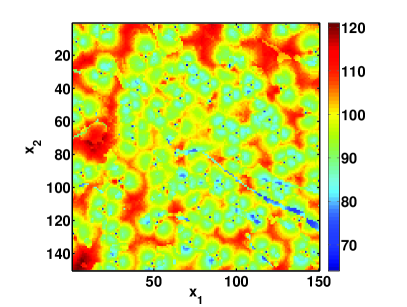
(a) True path-loss map.

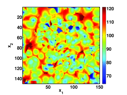
(b) Estimated path-loss map.

Figure 1: Visualization of original and snapshot of online-learned path-loss map in urban scenario.

A visual comparison of the both figures reveals significant similarities between the estimated and the original path-loss maps. The path-loss maps estimated by the base stations can now be used to provide predictions of path-loss conditions to particular users in the system. To confirm the first impression of good performance by Figure 1, we examine the estimation results along a route generated by the SUMO software between two arbitrary locations. Figure 2 illustrates the path-loss prediction for an exemplary route. While the dashed-dotted blue and red lines represent a particular sample of the predicted path-loss, obtained using APSM and the multikernel algorithm, respectively, the solid green lines represent the mean of the predicted path-loss traces (calculated from 100 runs of the simulation). In addition, we depict twice the standard error of the mean as shaded area around the mean, which is calculated for each time instant. Figure 2 compares the true path-loss evolution along the route with the predicted path-loss evolutions for the two algorithms. Note that the estimated path-loss values closely match the true ones. Furthermore, the estimation results are expected to improve for routes along frequently used roads owing to the large number of available measurements. For the sake of completeness, we additionally computed the MSE to complement Figure 2. By taking into account only the pixels that belong to the specific route, we obtain a (normalized) MSE (as defined in (23) of $0.0037$ for the APSM algorithm and $0.0027$ for the multikernel algorithm.

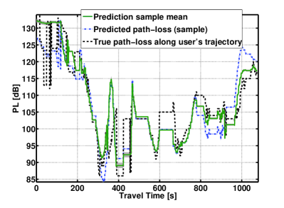
(a) APSM based prediction

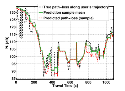
(b) Multikernel-based prediction

Figure 2: Comparison of true path-loss experienced by UOI and path-loss predicted by kernel-based methods in urban scenario.

Now we turn our attention to the question of how much time the algorithms require for sufficiently accurate estimation. To this end, we studied the evolution of the MSE over time. One result of this study is presented in Figure 3, where we observe a fast decrease of the MSE for both algorithms. The multikernel algorithm, however, outperforms APSM in terms of the MSE, with only a negligible loss in convergence speed.

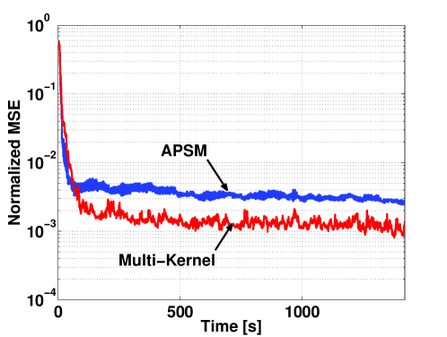
Figure 3: Comparison of the MSE performances in urban scenario.

As described in Section II, the measured value and the reported location can be erroneous. Therefore, it is essential for the algorithms to be robust against measurement errors. Figures 4(a) and 4(b) depict the impact of incorrect location reports and erroneous path-loss measurements on the MSE, respectively. This errors are chosen uniformly at random, with a variable maximum absolute value that is investigated in Figure 4. Note that a location error of less than $5\%$ means an offset in each reported coordinate of at most $375$ m (i.e., up to $8$ pixels). Such large errors are usually not encountered in modern GPS devices [31].

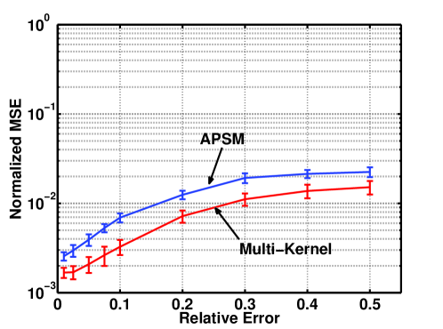
(a) Sensitiveness against errors in reported locations. The relative error is defined to be the maximum possible error in the measured coordinates (in meter) divided by the total dimension of the area ($7500\,\mathrm{m}$).

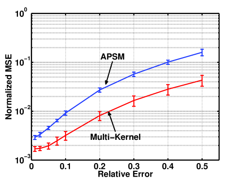
(b) Sensitiveness against errors in path-loss measurements. The relative error is the ratio of the maximum possible error per path-loss measurement to the average path-loss value (averaged over the path-loss values of all pixels).Thereby a relative error of $0.1$ corresponds to a maximum path-loss error of (roughly) $10\,\mathrm{dB}$.

Figure 4: Impact of errors on the MSE performance in urban scenario. Error bars represent 95% confidence intervals under the assumption that the sample average of the MSE after $5000\,\mathrm{s}$ is normally distributed.

From these simulations, we can conclude that both algorithms are robust to the relevant range of errors but they are more sensitive to path-loss measurement errors than to inaccurate location reports. In this particular scenario, we can also say that the multikernel algorithm is more robust than the APSM algorithm. Finally, we show that the multikernel algorithm achieves an accuracy similar to that of the APSM algorithm using a drastically smaller dictionary.

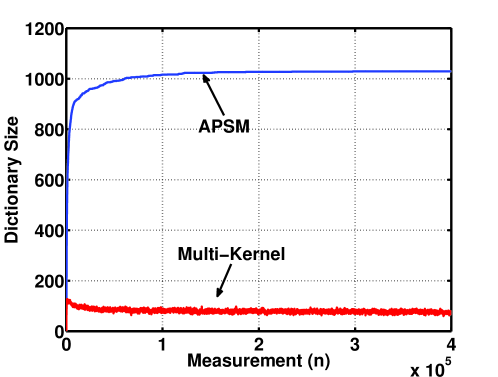
Figure 5: Comparison of dictionary sizes using APSM and multikernel approach with iterative weighting.

This can be concluded from Figure 5. For an exemplary simulation run, it shows that the evolution of the dictionary sizes over time for the APSM algorithm and the multikernel algorithm. We observe that the dictionary size of the multikernel algorithm is decreasing with the time, which is due to the block sparsity enforced by the second term in the cost function given by (10).

The parameters of the algorithms have been tailored to the scenario at hand to obtain the best possible estimation results. This, however, raises the question of how sensitive the estimation performance is to parameter changes. To provide insight into this problem, we performed experiments for selected parameters. As far as the APSM algorithm is concerned, the parameters are the tolerable error level $\varepsilon$ in (3), the step size $\mu$ of the update in (5), the measure of linear independency $\alpha$ (cf. [18, Section 5.3]), which is used for sparsification, and the kernel width $\sigma$ of the Gaussian kernel in (24). In case of the multikernel algorithm, we study the impact of the error level $\varepsilon_{\mathrm{MK}}$ in (9), the step size $\eta$, and the sparsification criterion $\delta$ (defined in [19, Equation 9]). Following the principle of $2^{k}$ factorial design [32], we chose for each parameter a very low value, indicated by the subscript $l$, and a very high value, indicated by the subscript $h$ (the particular parameter values are given in Tables IV and V).

TABLE IV: Parameter choice in Figure 6(a).

Parameter	$\epsilon_{\footnotesize{l,\text{APSM}}}$	$\epsilon_{h,\text{APSM}}$	$\mu_{l}$	$\mu_{h}$	$\alpha_{l}$	$\alpha_{h}$	$\sigma_{l}$	$\sigma_{h}$
Value	$0.0001$	$0.9$	$0.1$	$1.99$	$0.001$	$0.9$	$0.0001$	$1$

TABLE V: Parameter choice in Figure 6(b).

Parameter	$\epsilon_{l,\text{MK}}$	$\epsilon_{h,\text{MK}}$	$\eta_{l}$	$\eta_{h}$	$\delta_{l}$	$\delta_{h}$
Value	$0.0001$	$0.9$	$0.01$	$1.99$	$0.5$	$0.99999$

Then the algorithms were evaluated with all the parameter choices and the resulting estimation accuracy was compared to accuracy of the default choice.
The results are summarized in Figure 6. In particular, Figures 6(a) and 6(b) show the influence of important design parameters on the APSM algorithm and the multikernel algorithm, respectively.

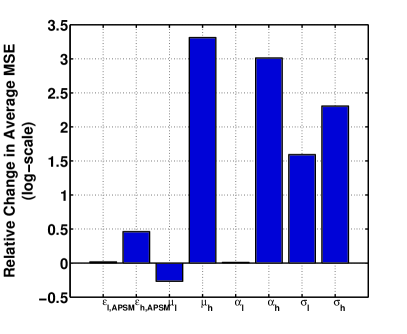
(a) APSM

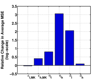
(b) Multi-kernel algorithm

Figure 6: Effect of the algorithm parameters on MSE in urban setting.

From these figures, we can conclude that the MSE can in general be improved by choosing a very small $\mu$ (cf. Figure 6(a)). However, these performance gains are in general achieved at the cost of a worse convergence speed, which is ignored in Figure 6. This observation is a manifestation of the known tradeoff between convergence speed versus steady-state performance of adaptive filters.

IV-C Campus network scenario

To demonstrate the capabilities of the proposed methods in a different setting, we now use the cu/cu_wart dataset available in the CRAWDAD project [33]. The dataset provides traces of received signal strength (RSS) measurements collected in a 802.11 network at the University of Colorado Wide-Area Radio Testbed, which spans an area of $1.8\times 1.4$ kilometers. These traces are measured at a high spatial resolution. In fact, over 80% of the measurements were taken less than 3 meters apart. Further details on the data, in particular on the measurement procedure, can be found at [33]. We used 70% of the data points (chosen uniformly at random) for training and the remaining 30% of the data points for testing and performance evaluation. This scenario has available less data than the previous urban scenario. This gives us the opportunity to compare the performance of our low-complexity online methods with (more complex) state-of-the-art batch-processing methods. With reduced data, numerical issues due to finite precision do not arise. In particular, we choose a popular method from geostatistics for comparison; namely, ordinary kriging [34]. For example, in [10], this method was applied to the estimation of radio maps (in particular, SNR maps).

Figure 7 illustrates the decay of the MSE for the APSM algorithm and the multikernel algorithm as the number of measurements increases. The MSE is calculated using only the test data points, which were not used in the learning process. We note that both algorithms behave as desired; the MSE decreases fast with the number of measurements. (Our methods perform only one iteration per measurement due to their online nature, but we may re-use training data points multiple times. Therefore, the number of measurements in Figure 7 is larger then the number of available training data points.) The multikernel approach seems to be outperformed by the APSM algorithm with respect to the convergence speed in this scenario. As shown in Section IV-B, this result does not seem to hold when the underlying data is more irregular. We see two reasons for this changing behavior. Both are related to the fact that the data of the Campus scenario is more regular than that of the Berlin scenario. The path-loss does not have sudden spatial changes. In this case, it is easier to tailor the parameters of the APSM method, and, in particular, the kernel width to the data at hand. In fact, with highly irregular data, a very narrow kernel is needed by the APSM to achieve good performance, which is detrimental to the convergence speed. In contrast, the multi-kernel algorithm has the advantage of offering multiple different kernels to adapt automatically to the data, without manual tuning of parameters.

Not only is the estimation quality important, but also the complexity, which grows fast with the amount of data and the number of kernels. Therefore, in order to reduce the complexity, we proposed in Section III-D an iterative weighting scheme that exploits sparsity of the multikernel algorithm. In addition to the comparison to APSM, Figure 7 indicates that our iterative weighting approach significantly outperforms that of [19] with respect to the convergence speed.

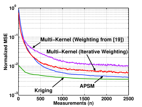
Figure 7: Comparison of kernel-based algorithms’ performance in CRAWDAD scenario. As a baseline, a curve based on a popular but non-realtime geostatistical method (kriging) is shown.

So far, we have only compared the two proposed kernel-based online learning schemes with each other. However, it is also of interest to compare the proposed methods with state-of-the-art approaches in the literature. Therefore, Figure 7 also includes the MSE performance of the kriging approach. We highlight that since kriging is essentially an offline scheme where all measurements have to be available beforehand, so a comparison is difficult and not entirely fair. In order to make a direct comparison possible, we apply the kriging technique at certain time instances with all (at those points in time) available measurements. Despite providing highly precise results given the amount of available measurements (see Figure 7), this method has a serious drawback, which is inherent to all batch methods: the computational complexity does not scale, because it grows fast with the number of data points available. In fact, all calculations have to be carried out from scratch as soon as a new measurement arrives. We apply an ordinary kriging estimator with a Gaussian semivariogram model. The most important simulation parameters can also be found in Table VI. The reader is referred to [34, 10] for further details.
In Figure 7, we can observe that the kriging scheme shows very good results even with few measurements, but from a certain point in time, more measurements do not significantly improve the quality of estimation. Moreover, we observe that our kernel-based schemes, after a sufficient number of measurements (i.e., iterations), can achieve almost the same level of accuracy, but at a much lower complexity and in an online fashion. To be more precise, we note that the kriging method needs to solve a dense system of linear equations in every iteration. This has a complexity of $O(n^{3})$ (with $n$ being the number of available samples). In addition, to obtain the results in Figure 7 a parametric semivariogram model needs to be fitted to the sample data (see [10] for details) which is a (non-convex) problem of considerable complexity.

TABLE VI: Simulation parameters for the campus network scenario

Simulation Parameter	Value
Number of unique data points	$1274$
Number of simulation runs	$100$
Amount of training data	$70\%$ of data points
Amount of test/validation data	$30\%$ of data points
Simulation duration (iterations)	2500
Semivariogram fitting model	Gaussian

V Conclusions

Based on the state-of-the-art framework for APSM-based and multikernel techniques, we have developed novel learning algorithms for the problem of reconstructing a path-loss map for any area covered by a large cellular network. In addition to path-loss measurements performed by sparsely and non-uniformly distributed mobile users, the proposed algorithms can smoothly incorporate side information to provide robust reconstruction results. Low-complexity is ensured by imposing sparsity on kernels and measurement data. Unlike current solutions based on measurements, the algorithms can operate in real time and in a distributed manner. Only to predict the path-loss for locations outside of the current cell of the user of interest, a data exchange between adjacent base stations becomes necessary.

As pointed out in the introduction, the path-loss information provided by the proposed algorithms can be used to reconstruct a complete coverage map for any area of interest. The accurate knowledge of coverage maps allows us to design robust schemes for proactive resource allocation. In particular, if combined with prediction of mobile users’ trajectories, the delay-tolerance of some applications can be exploited to perform spatial load balancing along an arbitrary trajectory for a better utilization of scarce wireless resources. The performance of such schemes can be further enhanced if, in addition to a path-loss map, the network load is predicted. This is an interesting and very promising research direction for future work.

References

- [1] C. Phillips, D. Sicker, and D. Grunwald, “A Survey of Wireless Path Loss Prediction and Coverage Mapping Methods,” Communications Surveys Tutorials, IEEE, vol. 15, no. 1, pp. 255–270, 2013.
- [2] R. Di Taranto, S. Muppirisetty, R. Raulefs, D. Slock, T. Svensson, and H. Wymeersch, “Location-Aware Communications for 5G Networks: How location information can improve scalability, latency, and robustness of 5G,” Signal Processing Magazine, IEEE, vol. 31, no. 6, pp. 102–112, Nov. 2014.
- [3] G. Fodor, E. Dahlman, G. Mildh, S. Parkvall, N. Reider, G. Miklos, and Z. Turanyi, “Design aspects of network assisted device-to-device communications,” IEEE Communications Magazine, vol. 50, no. 3, pp. 170–177, 2012.
- [4] J. Tadrous, A. Eryilmaz, and H. El Gamal, “Proactive Resource Allocation: Harnessing the Diversity and Multicast Gains,” Information Theory, IEEE Transactions on, vol. 59, no. 8, pp. 4833–4854, 2013.
- [5] M. Proebster, M. Kaschub, T. Werthmann, and S. Valentin, “Context-aware resource allocation for cellular wireless networks,” EURASIP Journal on Wireless Communications and Networking, vol. 2012, no. 1, p. 216, Jul. 2012. [Online]. Available: http://jwcn.eurasipjournals.com/content/2012/1/216
- [6] S. Theodoridis, K. Slavakis, and I. Yamada, “Adaptive Learning in a World of Projections,” Signal Processing Magazine, IEEE, vol. 28, no. 1, pp. 97–123, 2011.
- [7] C. Phillips, S. Raynel, J. Curtis, S. Bartels, D. Sicker, D. Grunwald, and T. McGregor, “The efficacy of path loss models for fixed rural wireless links,” in Passive and Active Measurement. Springer, 2011, pp. 42–51.
- [8] M. Piacentini and F. Rinaldi, “Path loss prediction in urban environment using learning machines and dimensionality reduction techniques,” Computational Management Science, vol. 8, no. 4, pp. 371–385, 2011. [Online]. Available: http://dx.doi.org/10.1007/s10287-010-0121-8
- [9] I. Popescu, I. Nafomita, P. Constantinou, A. Kanatas, and N. Moraitis, “Neural networks applications for the prediction of propagation path loss in urban environments,” in Vehicular Technology Conference, 2001. VTC 2001 Spring. IEEE VTS 53rd, vol. 1, 2001, pp. 387–391 vol.1.
- [10] D. M. Gutierrez-Estevez, I. F. Akyildiz, and E. A. Fadel, “Spatial Coverage Cross-Tier Correlation Analysis for Heterogeneous Cellular Networks,” IEEE Transactions on Vehicular Technology, vol. 63, no. 8, pp. 3917–3926, 2014.
- [11] E. Dall’Anese, S.-J. Kim, and G. B. Giannakis, “Channel gain map tracking via distributed Kriging,” IEEE Transactions on Vehicular Technology, vol. 60, no. 3, pp. 1205–1211, 2011.
- [12] J. Robinson, R. Swaminathan, and E. W. Knightly, “Assessment of urban-scale wireless networks with a small number of measurements,” in Proceedings of the 14th ACM international conference on Mobile computing and networking. ACM, 2008, pp. 187–198.
- [13] I. Yamada and N. Ogura, “Adaptive projected subgradient method for asymptotic minimization of sequence of nonnegative convex functions,” 2005.
- [14] B. T. Polyak, “Minimization of unsmooth functionals,” USSR Computational Mathematics and Mathematical Physics, vol. 9, no. 3, pp. 14–29, 1969.
- [15] A. H. Sayed, Fundamentals of adaptive filtering. John Wiley & Sons, 2003.
- [16] J. Shawe-Taylor and N. Cristianini, Kernel methods for pattern analysis. Cambridge university press, 2004.
- [17] P. Combettes and J.-C. Pesquet, “Proximal Splitting Methods in Signal Processing,” in Fixed-Point Algorithms for Inverse Problems in Science and Engineering, ser. Springer Optimization and Its Applications, H. H. Bauschke, R. S. Burachik, P. L. Combettes, V. Elser, D. R. Luke, and H. Wolkowicz, Eds. Springer New York, 2011, pp. 185–212. [Online]. Available: http://dx.doi.org/10.1007/978-1-4419-9569-8\_10
- [18] K. Slavakis and S. Theodoridis, “Sliding Window Generalized Kernel Affine Projection Algorithm Using Projection Mappings,” EURASIP Journal on Advances in Signal Processing, vol. 2008, no. 1, p. 735351, Apr. 2008. [Online]. Available: http://asp.eurasipjournals.com/content/2008/1/735351
- [19] M. Yukawa and R.-i. Ishii, “Online model selection and learning by multikernel adaptive filtering,” in Proc. 21st EUSIPCO, Marrakech, 2013.
- [20] I. Yamada, M. Yukawa, and M. Yamagishi, “Minimizing the Moreau envelope of nonsmooth convex functions over the fixed point set of certain quasi-nonexpansive mappings,” in Fixed-Point Algorithms for Inverse Problems in Science and Engineering. Springer, 2011, pp. 345–390.
- [21] M. Yukawa, “Multikernel Adaptive Filtering,” Signal Processing, IEEE Transactions on, vol. 60, no. 9, pp. 4672–4682, 2012.
- [22] E. J. Candes, M. B. Wakin, and S. P. Boyd, “Enhancing sparsity by reweighted ℓ 1 minimization,” Journal of Fourier Analysis and Applications, vol. 14, no. 5-6, pp. 877–905, 2008.
- [23] E. Pollakis, R. L. G. Cavalcante, and S. Stanczak, “Enhancing energy efficient network operation in multi-RAT cellular environments through sparse optimization,” in The IEEE 14th Workshop on Signal Processing Advances in Wireless Communications (SPAWC), Darmstadt, Germany, 2013.
- [24] B. Sriperumbudur, D. Torres, and G. Lanckriet, “A majorization-minimization approach to the sparse generalized eigenvalue problem,” Machine Learning, vol. 85, no. 1-2, pp. 3–39, 2011. [Online]. Available: http://dx.doi.org/10.1007/s10994-010-5226-3
- [25] O. L. Mangasarian, “Machine learning via polyhedral concave minimization,” in Applied Mathematics and Parallel Computing. Springer, 1996, pp. 175–188.
- [26] F. Rinaldi, “Concave programming for finding sparse solutions to problems with convex constraints,” Optimization Methods and Software, vol. 26, no. 6, pp. 971–992, 2011.
- [27] I. F. Gorodnitsky and B. D. Rao, “Sparse signal reconstruction from limited data using FOCUSS: A re-weighted minimum norm algorithm,” Signal Processing, IEEE Transactions on, vol. 45, no. 3, pp. 600–616, 1997.
- [28] MOMENTUM, “MOdels and siMulations for nEtwork plaNning and conTrol of UMts,” url{http://momentum.zib.de/}, 2004. [Online]. Available: http://momentum.zib.de
- [29] “OpenStreetMap,” 2014. [Online]. Available: www.openstreetmap.org
- [30] M. Behrisch, L. Bieker, J. Erdmann, and D. Krajzewicz, “SUMO - Simulation of Urban MObility: An Overview,” in SIMUL 2011, The Third International Conference on Advances in System Simulation, Barcelona, Spain, 2011.
- [31] CSR, “SiRFstarIII™ GSC3e/LPx & GSC3f/LPx Product Sheet,” Data Sheet, 2013. [Online]. Available: http://www.csr.com/products/27/sirfstariii-gsc3elpx-gsc3flpx
- [32] A. M. Law and W. D. Kelton, Simulation modeling and analysis, 3rd ed. McGraw-Hill, Inc., 2000.
- [33] “{CRAWDAD} data set cu/cu_wart (v. 2011-10-24),” Downloaded from http://crawdad.org/cu/cu_wart/, 2011.
- [34] C. Phillips, M. Ton, D. Sicker, and D. Grunwald, “Practical radio environment mapping with geostatistics,” in Dynamic Spectrum Access Networks (DYSPAN), 2012 IEEE International Symposium on. IEEE, 2012, pp. 422–433.