Analysis of Petri Net Models through Stochastic Differential Equations

Abstract

It is well known, mainly because of the work of Kurtz, that density dependent Markov chains can be approximated by sets of ordinary differential equations (ODEs) when their indexing parameter grows very large. This approximation cannot capture the stochastic nature of the process and, consequently, it can provide an erroneous view of the behavior of the Markov chain if the indexing parameter is not sufficiently high. Important phenomena that cannot be revealed include non-negligible variance and bi-modal population distributions. A less-known approximation proposed by Kurtz applies stochastic differential equations (SDEs) and provides information about the stochastic nature of the process.

In this paper we apply and extend this diffusion approximation to study stochastic Petri nets. We identify a class of nets whose underlying stochastic process is a density dependent Markov chain whose indexing parameter is a multiplicative constant which identifies the population level expressed by the initial marking and we provide means to automatically construct the associated set of SDEs. Since the diffusion approximation of Kurtz considers the process only up to the time when it first exits an open interval, we extend the approximation by a machinery that mimics the behavior of the Markov chain at the boundary and allows thus to apply the approach to a wider set of problems. The resulting process is of the jump-diffusion type. We illustrate by examples that the jump-diffusion approximation which extends to bounded domains can be much more informative than that based on ODEs as it can provide accurate quantity distributions even when they are multi-modal and even for relatively small population levels. Moreover, we show that the method is faster than simulating the original Markov chain.

1 Introduction

Stochastic Petri Nets (SPNs) are a well-known formalism widely used for the performance analysis of complex Discrete Event Dynamic Systems [1, 3]. The advantages of modeling with SPNs include their well defined time semantics which often allows the direct definition of the Continuous Time Markov Chain (CTMC) that represents the SPN’s underlying stochastic process whose state space is isomorphic to the reachability set of the net. The analysis of real systems often requires the construction of SPN models with huge state spaces that may hamper the practical relevance of the formalism and have motivated the development of many techniques capable of reducing the impact of this problem. However, when the model includes large groups of elements (e.g., Internet users, human populations, molecule quantities) most of these techniques may turn out to be insufficient, so that expected values and probability distributions must be estimated with Discrete Event Simulation [7, 8]. An alternative to simulation is the approximation of the stochastic model with a deterministic one in which its time evolution is represented with a set of Ordinary Differential Equations (ODEs) whose solution is interpreted as the approximate expected value of the quantities of interest.

The convergence of the solution of the system of ODEs to the expected values of their corresponding quantities, when the sizes of the involved populations grow very large has been the subject of many papers. Most of these are based on the work of Kurtz [13] and have shown that the accuracy of its approximation is acceptable when the model represents a system of large interacting population quantities [18, 19]. Unfortunately, there are many cases in which the deterministic approximation is not satisfactory because the obtained approximate expected values give little or even erroneous information about the actual population levels. This happens either when the population sizes are not large enough to rule out the variability of the process and the obtained expected values are not reliable, or when the population distributions are multi-modal, a case in which the mean does not provides much information [17].

In this paper we extend a stochastic approximation of the CTMC that has been introduced in [14] by Kurtz. There, the fluidisation is augmented by a suitable noise term which accounts for the stochasticity of the original system yielding a system of Stochastic Differential Equations (SDEs). Unfortunately the proposed diffusion approximation is only valid up to the first time the system exits a suitable open domain. In real systems however the boundaries of the state space are repeatedly visited (the buffer of a queue may get full, all resources of a system may be in use) and the system can stay there for a finite time and come back to the interior again and again. In these cases, the diffusion approximation proposed in [14] gives a totally incomplete description. We propose an improved approximation which results in a jump diffusion process that visits the boundaries and with jumps that push back the process to the interior of its state space.

The paper is organized as follows. In Section 2, in order to provide the theoretical background of our exposition, we review some of Kurtz’s results regarding deterministic and diffusion approximations. In Section 3 we apply these results to SPNs and extend Kurtz’s results to treat the barriers of the state space. Numerical experiments are provided in Section 4 and conclusions are drawn in Section 5.

2 Two fluid approximations for density dependent CTMCs

In this section we give a brief overview of two possible approximations of density dependent CTMCs. Both of these are “fluid” in the sense that the state space of the approximating process is continuous. The first one is the well-known deterministic fluid limit introduced in [13] which employs a set of ordinary differential equations. The second one is the so-called diffusion approximation introduced in [14] which uses SDEs. The decisive difference between the two approximations is that, at any time, the first one provides a single number per random variable of interest (e.g., number of customers in service, number of molecules in a cell), which is usually interpreted as the approximate expected value, while the second one leads to an approximate joint distribution of all the variables of interest.

2.1 Density dependent CTMCs

In the following we will denote $\mathbb{R}$, $\mathbb{Z}$ and $\mathbb{N}$ the set of real, integer and natural numbers, respectively. Given a positive constant, $r$, we will denote by $\mathbb{R}^{r}$ the $r$–dimensional cartesian product of the space $\mathbb{R}$. The letter $u$ will be dedicated to the time index ranging continuously between $[0,+\infty)$ or $[0,T]$ when specified. The discrete states of a continuous time Markov chain will be denoted as $k$ or $h$ and range in the state space that is included in $\mathbb{Z}^{r}$. We will always consider the abstract probability space to be given as $(\Omega,\mathcal{F},\mathbb{P})$, where $\mathbb{P}$ is the probability measure. Furthermore, $\mathbb{E}$ will denote the expectation with respect to $\mathbb{P}$.

Definition 1

A family of Markov chains $X^{[N]}(u)$ with indexing parameter $N$ and with state space $S^{[N]}\subseteq\mathbb{Z}^{r}$, is called density dependent iff there exists a continuous non-zero function $f:\mathbb{R}^{r}\times\mathbb{Z}^{r}\rightarrow\mathbb{R}$ such that the instantaneous transition rate (intensity) from state $k$ to state $k+l$ can be written as

$$q^{[N]}_{k,k+l}=Nf\left(\frac{k}{N},l\right),\quad l\neq 0.$$ (1)

In the previous definition, the first argument of the function $f$ can be seen as a normalized state (with respect to the indexing parameter $N$) of the CTMC and the second argument as a vector that describes the effect of a transition (change of state). Consequently, eq. (1) states that, given a vector $l$, the intensities depend on the normalized state, $k/N$, and are proportional to the indexing parameter $N$. In the following we denote the set of possible state changes by $C$, i.e., $C=\{l:l\in\mathbb{Z}^{r},l\neq 0,q^{[N]}_{k,k+l}\neq 0\}$.

Some important models do not satisfy Definition 1 exactly but are still treatable in the same framework. For this reason we introduce the following more general definition.

Definition 2

A family of Markov chains $X^{[N]}(u)$ with parameter $N$ and with state space $S^{[N]}\subseteq\mathbb{Z}^{r}$, is called nearly density dependent iff there exists a continuous non-zero function $f:\mathbb{R}^{r}\times\mathbb{Z}^{r}\rightarrow\mathbb{R}$ such that the instantaneous transition rate (intensity) from state $k$ to state $k+l$ can be written as:

$$q^{[N]}_{k,k+l}=N\left[f\left(\frac{k}{N},l\right)+O\left(\frac{1}{N}\right)\right],\quad l\neq 0.$$ (2)

Example 1

As an example consider a closed network of $r$ infinite server queues with exponential service time distributions and with $N$ jobs circulating in it. The state space is thus $S^{[N]}=\{k:k\in\mathbb{Z}^{r},0\leq k_{i}\leq N,\sum_{i}k_{i}=N\}$. Let $\mu_{i}$ denote the service intensity of the $i$th queue, $r_{i,j}$ the routing probabilities with $r_{i,i}=0$, and $l_{i,j},i\neq j,$ a vector with $-1$ in position $i$, $+1$ in position $j$ and 0s elsewhere. Then the transition rates and the functions $f$ are

$$q^{[N]}_{k,k+l}=\left\{\begin{array}[]{ll}k_{i}\mu_{i}r_{i,j}&\mbox{if}~{}l=l_{i,j}\\ 0&\mbox{otherwise}\end{array}\right. \quad\quad f(y,l)=\left\{\begin{array}[]{ll}y_{i}\mu_{i}r_{i,j}&\mbox{if}~{}l=l_{i,j}\\ 0&\mbox{otherwise}\end{array}\right.$$ (7)

and thus that the transition rates are in the form given in eq. (1), with $y=k/N$. For this simple example the transition rates depend only on one component of the state. This is not a necessary condition for a CTMC to be density dependent and in Section 4 we show examples for which this condition does not hold.

In order to gain a better understanding of the property of density dependence, let us introduce some general concepts from the theory of Markov chains. Among the many books devoted to this topic, we refer the reader to [6].

For a general Markov chain $M(u)$ with state space $S\subseteq\mathbb{Z}^{r}$ and instantaneous transition rates $q_{k,h}$, let us introduce the following key object

$$F_{M}(k)=\sum_{h\in S}(h-k)q_{k,h}\quad k\in S.$$ (8)

The function $F_{M}$ will be referred to as the generator of the chain. Under suitable hypothesis the expectation of $M(u)$ solves the following Dynkin equation cf. [6, Chapter 9, Theorem 2.2]

$$\frac{d\mathbb{E}[M(u)]}{du}=\mathbb{E}[F_{M}(M(u))].$$ (9)

Example 2

For the density dependent CTMC introduced in Example (1), the $m$th entry of the generator is

$$(F_{X^{[N]}}(k))_{m}=\sum_{i=1,i\neq m}^{r}k_{i}\mu_{i}r_{i,m}-k_{m}\mu_{m}$$

Define by $\pi_{k}(u)$ the transient probabilities and apply the Dynkin equation. We obtain

$$\frac{d(\mathbb{E}[M(u)])_{m}}{du}= \sum_{k\in E_{N}}\pi_{k}(u)\left(\sum_{i=1,i\neq m}^{r}k_{i}\mu_{i}r_{i,m}-k_{m}\mu_{m}\right)$$

$$= \sum_{i=1,i\neq m}^{r}(\mathbb{E}[M(u)])_{i}\mu_{i}r_{i,m}-(\mathbb{E}[M(u)])_{m}\mu_{m}$$

which provides a set of ODEs that can be used to calculate the mean queue length of each queue. Note that in general it is not the case that applying the Dynkin equation leads to such ODEs from which the mean quantities can be directly obtained.

In order to bring to the same scale the state spaces of all the CTMCs $X^{[N]}(u)$, it may be convenient to introduce the family of normalized CTMCs as $Z^{[N]}(u)=\frac{X^{[N]}(u)}{N}$, which is also referred to as the density process. Notice that the density process will have state space $\left\{\frac{k}{N},k\in\mathbb{Z}^{r}\right\}$. Two invariance properties of density dependent CTMCs can then be stated using the normalized chains.

Property 1

If the set of possible state changes $C$ does not depend on $N$, the density dependence property of the family $X^{[N]}(u)$ is equivalent to require that for the family of the normalized CTMCs, $Z^{[N]}(u)$, the generator does not depend on $N$. Indeed

$$F_{Z^{[N]}}\left(\frac{k}{N}\right)=\sum_{l\in C}\frac{l}{N}\cdot p^{[N]}_{\frac{k}{N},\frac{k}{N}+\frac{l}{N}}=\sum_{l\in C}\frac{l}{N}\cdot q^{[N]}_{k,k+l}=\sum_{l\in C}lf\left(\frac{k}{N},l\right)=F\left(\frac{k}{N}\right)$$ (10)

where $p^{[N]}_{\frac{k}{N},\frac{h}{N}}$ and $q^{[N]}_{k,h}$ are the instantaneous transition rates of the processes $Z^{[N]}$ and $X^{[N]}$, respectively. Hence, if the increments $l$ are constant with $N$, i.e. the set $C$ does not depend on $N$ and comprises elements which are all independent of $N$, the generator is a function that depends on $N$ only through the state $\frac{k}{N}$. Let us notice that if the family $X^{[N]}(u)$ is only nearly density dependent then $F_{Z^{[N]}}\left(\frac{k}{N}\right)=F\left(\frac{k}{N}\right)+O\left(\frac{1}{N}\right)$.

Property 2

Each element of the family $Z^{[N]}$ solves the same Dynkin equation

$$\frac{d\mathbb{E}[Z^{[N]}(u)]}{du}=\mathbb{E}[F(Z^{[N]}(u))].$$ (11)

The results reported in the following two subsections was demonstrated by Kurtz exploiting the above properties.

2.2 From CTMCs to ODEs

In [13] Kurtz has shown that given a nearly density dependent family of CTMCs $X^{[N]}(u)$, if $\lim_{N\rightarrow\infty}Z^{[N]}(0)=z_{0}$, then, under relatively mild conditions on the generator $F$ given in eq.(10), the density process $Z^{[N]}$ converges (in a sense to be precised) to a deterministic function $z$ which solves the ODE

$$dz(u) =F(z(u))du,\quad\quad z(0)=z_{0}.$$ (12)

In [13] the following convergence in probability is used: for every $\delta>0$

$$\lim_{N\rightarrow\infty}\mathbb{P}\left\{\sup_{u\leq T}\left|Z^{[N]}(u)-z(u)\right|>\delta\right\}=0.$$ (13)

where $T$ is the upper limit of the finite time horizon.

The function $z(u)$ is usually interpreted as the asymptotic mean of the process as it solves an equation which is analogous to eq. (11). The difference $Z^{[N]}(u)-z(u)$ can be interpreted as the “noisy” part of $Z^{[N]}(u)$. It was shown in [13] that for $N\rightarrow\infty$ the density process $Z^{[N]}(u)$ flattens at its mean value and that the magnitude of the noise is

$$Z^{[N]}(u)-z(u)=O\left(\frac{1}{\sqrt{N}}\right).$$ (14)

The result expressed by eq.(13) is often used to approximate the density dependent process $X^{[N]}(u)=NZ^{[N]}(u)$ with the deterministic function $x^{[N]}(u)=Nz(u)$, in case of a finite $N$. In doing so, this approximation disregards the noise term which is now of order $\sqrt{N}$ that is small compared with the order of the mean (that is $N$), but not in absolute terms. Moreover, it ignores every details of the probability distribution of $X^{[N]}(u)$ except for the mean. It is easy to see that there are cases, e.g., multi-modal distributions, where the mean gives too little information about the location of the probability mass, cf [17].

Let us stress that the convergence holds only if $\lim_{N\rightarrow\infty}Z^{[N]}(0)=z_{0}$, meaning that the corresponding sequence of initial conditions $X^{[N]}(0)$ needs to grow linearly with $N$. In particular if $X^{[N]}(u)$ is multivariate, each component should grow with the same rate.

2.3 From CTMCs to SDEs

An approximation of a density dependent family $X^{[N]}$ which preserves its stochastic nature and has a better order of convergence was proposed in [14, 15]. It has been shown in [14] that, given an open set $S\subset\mathbb{R}^{r}$, the density process $Z^{[N]}$ can be approximated by the diffusion process $Y^{[N]}$ with state space $S$ and solution of the following SDE

$$dY^{[N]}(u)=F(Y^{[N]}(u))du+\sum_{l\in C}\frac{l}{\sqrt{N}}\sqrt{f(Y^{[N]}(u),l)}\;dW_{l}(u)$$ (15)

where $W_{l}$ are independent standard one-dimensional Brownian motions and $f$ is given in eq. (1). The approximation holds up to the first time $Y^{[N]}$ leaves $S$. A rigorous mathematical treatment of SDEs can be found in [11]. In the physical literature the notation $\frac{dW(u)}{du}=\xi(u)$ is often used even if Brownian motion is nowhere differentiable and $\xi(u)$ is called a gaussian white noise. This SDE approach that goes back to the already cited [14, 15] has been applied in many contexts, e.g., it is used under the name of Langevin equations to model chemical reactions in [9].

The structure of eq. (15) is the following: the first term is the same that appears in eq. (12), while the second term represents the contribution of the noise and is responsible for the stochastic nature of the approximating process $Y^{[N]}$. A further relation between eq. (15) and eq. (12) can be obtained by considering that the stochastic part of the equation is proportional to $1/\sqrt{N}$, meaning that as $N\rightarrow\infty$ this term becomes negligible and $Y_{\infty}(u)$ solves the same ODE written in eq. (12). Let us remark that the construction of such noise is not based on an ad hoc assumption, but is derived from the structure of the generator of the original Markov chain.

As for the relation between the diffusion approximation and the original density process, in [14], it has been proven that, for any finite $N$, we have

$$Z^{[N]}(u)-Y^{[N]}(u)=O\left(\frac{\log N}{N}\right)$$ (16)

which, compared to eq. (14), is a better convergence rate. Thus, the processes $NY^{[N]}(u)$ approximates the density dependent CTMCs $X^{[N]}(u)$ with an error of order $\log N$, much better than the $\sqrt{N}$ of the deterministic fluid approximation.

Finally, let us stress that the approximation is valid only up to the first exit time from the open set $S$. For many applications the natural state space is bounded and closed and the process may reach the boundary of $S$ in a finite time $\tau$ with non-negligible probability. In such cases, since the approximating process $Y^{[N]}(u)$ is no longer defined for any $u\geq\tau$, this approximation is not applicable. To overcome this limitation suitable boundary conditions must be set and this problem, that was considered neither in [14] nor in [15], will be tackled in Section 3.4, representing our main contribution.

3 From SPNs to fluid approximations

In this section we first introduce stochastic Petri nets and give a condition under which their underlying CTMC is density dependent. Then, we reinterpret the results discussed in Section 2.2 and 2.3 in terms of SPNs. Finally, we extend the diffusion approximation to bounded domains by adding jumps to the diffusion that mimics the behavior of the original CTMC at the barrier.

3.1 Density dependent SPNs

Petri Nets (PNs) are bipartite directed graphs with two types of nodes: places and transitions. The places, graphically represented as circles, correspond to the state variables of the system (e.g., number of jobs in a queue), while the transitions, graphically represented as rectangles, correspond to the events (e.g., service of a client) that can induce state changes. The arcs connecting places to transitions (and vice versa) express the relations between states and event occurrences. Places can contain tokens (e.g., jobs) drawn as black dots within the places. The state of a PN, called marking, is defined by the number of tokens in each place. The evolution of the system is given by the occurrence of enabled transitions, where a transition is enabled iff each input place contains a number of tokens greater or equal than a given threshold defined by the multiplicity of the corresponding input arc. A transition occurrence, called firing, removes a fixed number of tokens from its input places and adds a fixed number of tokens to its output places (according to the multiplicity of its input/output arcs).

The set of all the markings that the net can reach, starting from the initial marking through transition firings, is called the Reachability Set (RS). Instead, the dynamic behavior of the net is described by means of the Reachability Graph (RG), an oriented graph whose nodes are the markings of the RS and whose arcs represent the transition firings that produce the corresponding marking changes.

Stochastic Petri Nets (SPNs) are PNs where the firing of each transition is assumed to occur after a delay (firing time) from the time it is enabled. In SPNs these delays are assumed to be random variables with negative exponential distributions [16]. Each transition of an SPN is thus associated with a rate that represents the parameter of its firing delay distribution. Firing rates may be marking dependent. When a marking is entered an exponentially distributed random delay is sampled for each enabled transition according to its intensity. The transition with the lowest delay fires and the system changes marking accordingly.

Here we recall the notation and the basic definitions used in the rest of the paper.

Definition 3

A stochastic Petri net (SPN) system is a tuple $\mathcal{N}=(P,T,I,O,\mathbf{m}_{0},\lambda)$:

• $P=\{p_{i}\}_{1\leq i\leq n_{p}}$ is a finite and non empty set of places.

• $T=\{t_{i}\}_{1\leq i\leq n_{t}}$ is a finite, non empty set of transitions with $P\cap T=\emptyset$.

• $I,O:P\times T\rightarrow\mathbb{N}$ are the input, output functions that define the arcs of the net and that specify their multiplicities.

• ${\bf m_{0}}:P\rightarrow\mathbb{N}$ is a multiset on $P$ representing the initial marking,

• $\lambda:T\rightarrow\mathbb{R}$ gives the firing intensity of the transitions.

The overall effect of a transition is described by the function $L=O-I$. The values assumed by the function $I,O$ and $L$ can be collected in $n_{p}\times n_{t}$ matrices (which we still call $I,O$ and $L$) whose entries are $I(p_{i},t_{j}),O(p_{i},t_{j})$ and $L(p_{i},t_{j})$, respectively. By $I(t)$ we denote the column of $I$ corresponding to transition $t$ (the same holds for $O$ and $L$). The matrix $L=O-I$ is called the incidence matrix.

A marking (or state) ${\bf m}$ is a function ${\bf m}:P\rightarrow\mathbb{N}$ identified with a multiset on $P$ which can be seen also as a vector in $\mathbb{N}^{n_{p}}$. A transition $t$ is enabled in marking $\mathbf{m}$ iff $\mathbf{m}(p)\geq I(p,t)$, $\forall p\in P$ where $\mathbf{m}(p)$ represents the number of tokens in place $p$ in marking $\mathbf{m}$. Enabled transitions may fire, so that the firing of transition $t$ in marking $\mathbf{m}$ yields a new marking $\mathbf{m}^{\prime}=\mathbf{m}-{I(t)}^{T}+{O(t)}^{T}=\mathbf{m}+{L(t)}^{T}$. Marking $\mathbf{m}^{\prime}$ is said to be reachable from $\mathbf{m}$ because of the firing of $t$ and is denoted by $\mathbf{m}{[{t}\rangle}\mathbf{m}^{\prime}$. The firing of a sequence ${\sigma}$ of transitions enabled at $\mathbf{m}$ and yielding $\mathbf{m}^{\prime}$ is denoted similarly: $\mathbf{m}{[{{\sigma}}\rangle}\mathbf{m}^{\prime}$.

Let $E(\textup{{{m}}})$ be the set of transitions enabled in marking $\mathbf{m}$. The enabling degree of transition $t$ in marking $\mathbf{m}$ is defined as

$$\forall t\in E(\textup{{{m}}}):\;e(t,\textup{{{m}}})=\min_{j:I(p_{j},t)\not=0}\left\lfloor\frac{\textup{{{m}}}(p_{j})}{I(p_{j},t)}\right\rfloor.$$ (17)

which implies that a transition $t\in E(\mathbf{m})$ is enabled in marking $\mathbf{m}-(e(t,\mathbf{m})-1)I(t)^{T}$, but not in marking $\mathbf{m}-e(t,\mathbf{m})I(t)^{T}$. The notion of enabling degree is particularly useful when a transition intensity is proportional to the number of tokens in the input places of the transition, i.e., when the transition models the infinite server mechanism [1].

In the CTMC that underlies the behavior of an SPN, states are identified with markings and a change of marking of the SPN corresponds to a change of state of the CTMC. If we assume that all the transitions of the SPN use an infinite server policy, then the transition rate from state $\mathbf{m}$ to state $\mathbf{m}^{\prime}$ in the CTMC can be written as

$$q_{\textup{{{m}}},\textup{{{m}}}^{\prime}}=\sum_{t:L(t)=(\textup{{{m}}}^{\prime}-\textup{{{m}}})}\lambda(t)e(t,\textup{{{m}}})$$ (18)

where $\lambda(t)$ depends only on the transition and the marking dependence is determined by the enabling degree $e(t,\textup{{{m}}})$.

A vector $\nu\in\mathbb{N}^{n_{p}}$ is called a P–semiflow of the SPN if it satisfies $\nu\,L=0$. All P–semiflows of an SPN can be obtained as linear combination of the P–semiflows that are elements of a minimal set. Given a marking m, the quantities $\textup{{{m}}}\,\nu^{T}$ are invariant and hence equal to $\textup{{{m}}}_{0}\,\nu^{T}$ where $\textup{{{m}}}_{0}$ is the initial marking.

Proposition 1

Let $\mathcal{N}=(P,T,I,O,\mathbf{m}_{0},\lambda)$ be an SPN model where all places are covered by P–semiflows and all transitions use an infinite server policy. Let us consider the family $\mathcal{N}^{[N]}$ of SPN models with indexing parameter $N$ obtained from $\mathcal{N}$ by considering an increasing sequence of initial markings $\textup{{{m}}}_{0}^{[N]}=N\alpha$ for a given vector $\alpha$. The corresponding family of CTMCs is nearly density dependent and the marking in each place has a bound which grows at most linearly with $N$. If the multiplicity of the input arcs are all unitary, the family is also density dependent.

Proof

Let $\{\nu^{(\eta)}\}_{\eta=1}^{\kappa}$ denote a minimal set of P–semiflows for $\mathcal{N}$ and, consequently, for any $\mathcal{N}^{[N]}$ (P–semiflows are independent of the initial marking). For each place the marking is bounded by

$$\textup{{{m}}}(p_{j})\leq\min_{\eta:\nu^{(\eta)}_{j}\neq 0}\left\{\frac{\textup{{{m}}}^{[N]}_{0}\nu^{(\eta)\,T}}{\nu^{(\eta)}_{j}}\right\}=N\min_{\eta:\nu^{(\eta)}_{j}\neq 0}\left\{\frac{\alpha\nu^{(\eta)\,T}}{\nu^{(\eta)}_{j}}\right\},$$ (19)

where $\nu^{(\eta)}_{j}$ is the component of the P–semiflow vector $\nu^{(\eta)}$ that corresponds to the place $p_{j}$. By eq. (18) and (17)

$$q_{\textup{{{m}}},\textup{{{m}}}+l}=\sum_{t:L(t)=l}\lambda(t)\min_{j:I(p_{j},t)\not=0}\left\lfloor\frac{\textup{{{m}}}(p_{j})}{I(p_{j},t)}\right\rfloor.$$

For any $j$ we have

$$\left\lfloor\frac{\textup{{{m}}}(p_{j})}{I(p_{j},t)}\right\rfloor=\frac{\textup{{{m}}}(p_{j})}{I(p_{j},t)}-\frac{R_{j}}{I(p_{j},t)},$$

where $R_{j}<I(p_{j},t)$ is the remainder of the division of $\textup{{{m}}}(p_{j})$ by $I(p_{j},t)$. So

$$q_{\textup{{{m}}},\textup{{{m}}}+l}= N\sum_{t:L(t)=l}\lambda(t)\min_{j:I(p_{j},t)\not=0}\left\{\frac{\textup{{{m}}}(p_{j})}{NI(p_{j},t)}-\frac{R_{j}}{N}\right\}$$

$$= N\left[\sum_{t:L(t)=l}\lambda(t)\min_{j:I(p_{j},t)\not=0}\left\{\frac{\textup{{{m}}}(p_{j})}{NI(p_{j},t)}\right\}+O\left(\frac{1}{N}\right)\right].$$

By Definition 2, the proposition follows. Notice that when the input arcs are all unitary the remainder is null, $R_{j}=0$ for any $j$, and hence the term disappears and the chain is density dependent.

Let us notice that the hypothesis $\textup{{{m}}}_{0}^{[N]}=N\alpha$ implies that the initial number of tokens in any place should grow with the same rate $N$. This means that a family of systems with finite resources cannot be modeled in this framework.

As shown in the proof of Proposition 1, for an SPN in which all places are covered by a P–semiflow, the number of tokens in a place is bounded. The minimal and maximal number of tokens in place $p_{i}$ will be denoted by $\mbox{MIN}(p_{i})$ and $\mbox{MAX}(p_{i})$, respectively. If $S^{[N]}$ denotes the state space of the CTMC associated to the SPN $\mathcal{N}^{[N]}$, then

$$\mbox{MIN}(p_{i})=\min_{x\in S^{[N]}}\;x_{i},~{}\mbox{MAX}(p_{i})=\max_{x\in S^{[N]}}\;x_{i},$$

where $x_{i}$ denotes the $i$–th component of the vector $x\in S^{[N]}$. The following set is a (possibly improper) superset of $S^{[N]}$

$$\hat{S}^{[N]}=\left\{x\in\mathbb{Z}^{n_{p}}:\forall i,\mbox{MIN}(p_{i})\leq x_{i}\leq\mbox{MAX}(p_{i})\mbox{ and }\forall\eta,x\nu^{(\eta)T}=\textup{{{m}}}_{0}\nu^{(\eta)T}\right\}.$$ (20)

which will help us to define the state space of the approximate models.

3.2 From SPNs to ODEs

Having characterized, in Proposition 1, a family of SPNs whose underlying CTMC family is nearly density dependent, we can apply the results reported in Section 2.2 to construct an approximation by ODEs. In order to provide a direct relation between the SPN family and the ODE approximation, we construct the approximation not for the normalized process $Z^{[N]}$, as it was done by Kurtz, but for the unnormalized $X^{[N]}$.

The state of the system in the ODE approximation will be denoted by $x^{[N]}(u)\in\mathbb{R}^{n_{p}}$. A given infinite server transition $t_{i}$ moves “fluid” tokens in state $x^{[N]}(u)$ with speed

$$\sigma(t_{i},x^{[N]}(u))=\lambda(t_{i})\min_{j:I(p_{j},t_{i})\not=0}\frac{x^{[N]}_{j}(u)}{I(p_{j},t_{i})}$$ (21)

which depends on the rate of the transition, $\lambda(t_{i})$, and on its enabling degree, calculated now at the “fluid” state. The number of tokens in the $i$-th place is then approximated by the following ODE system:

$$dx^{[N]}_{i}(u)=\sum_{j=1}^{n_{t}}\sigma(t_{j},x^{[N]}(u))L(p_{i},t_{j})du$$ (22)

so that if place $p_{i}$ is an input (output) place of transition $t_{j}$, then transition $t_{j}$ is removing (adding) tokens from (to) place $p_{i}$ according to the current speed of the transition and the multiplicity given by function $I$ ($O$).

It is easy to see that the ODE approximation maintains the same invariance properties, expressed by the P–semiflows, that the original SPN enjoys. Therefore the ODE system is redundant and each P–semiflow in the minimal set can be used to derive one of its components from the others and hence the system can be reduced by as many equations as the number of P–semiflows in the minimal set.

The fluid state space $\hat{G}^{[N]}\in\mathbb{R}^{n_{p}}$ of the deterministic approximation $x^{[N]}$ is

$$\hat{G}^{[N]}=\left\{x\in\mathbb{R}^{n_{p}}:\forall i,\mbox{MIN}(p_{i})\leq x_{i}\leq\mbox{MAX}(p_{i})\mbox{ and }\forall\eta,x{\nu^{(\eta)}}^{T}=\textup{{{m}}}_{0}{\nu^{(\eta)}}^{T}\right\}$$ (23)

that is the convex hull of the set $\hat{S}^{[N]}$ given in eq. (20). Theoretically, the fluid approximation may visit all the points between the boundaries that are compatible with the P–semiflows and the initial markings (gaps are filled). In practice, however, as the model follows a deterministic trajectory, only a $n_{p}$ dimensional curve is covered. Moreover, if the initial marking belongs to the interior of $\hat{G}^{[N]}$, denoted by $\mathring{G}^{[N]}$, where all the components are strictly between the bounds, then the approximation cannot visit the boundary defined as

$$\accentset{\star}{G}^{[N]}=\{x\in\hat{G}^{[N]}:x_{i}=\text{MAX}(p_{i})\text{ or }x_{i}=\text{MIN}(p_{i}),\text{for at least one }i.\}$$ (24)

3.3 From SPNs to SDEs

Under the hypothesis of density dependence, the procedure illustrated in Section 2.3 can be applied in this case too, and the number of tokens in each place can be approximated by the diffusion process $\Upsilon^{[N]}(u)=NY^{[N]}(u)$, with components $\Upsilon^{[N]}_{i}$ given by the following system of SDEs:

$$d\Upsilon^{[N]}_{i}(u)=\sum_{j=1}^{n_{t}}\sigma(t_{j},\Upsilon^{[N]}(u))L(p_{i},t_{j})du+\sum_{j=1}^{n_{t}}\sqrt{\sigma(t_{j},\Upsilon^{[N]}(u))}L(p_{i},t_{j})dW_{j}(u)$$ (25)

where each $W_{j}$ is an independent one-dimensional Brownian motion.

Just like the ODE approximation, also the diffusion approximation enjoys the invariance properties present in the SPN. Thus the size of the system can be reduced by removing one equation for each minimal P–semiflow.

As already remarked, the diffusion approximation $Y^{[N]}$ introduced in Section 2.3 is defined only up to the first exit from an open set and the same holds for $\Upsilon^{[N]}$. The natural state space for the process $\Upsilon^{[N]}$ would be the closed set $\hat{G}^{[N]}$ as defined in eq. (23). However the diffusion approximation is only valid up to the first exit from $\mathring{G}^{[N]}$. If the underlying CTMC is only nearly density dependent a suitable extension of approximation (25) can still be applied.

3.4 From SPNs to SDEs in bounded domains

We have already stressed that for an SPN model satisfying the hypothesis of Proposition 1 the number of tokens in each place is bounded between a minimal and a maximal value. In many real examples the CTMC visits some of the states corresponding to a minimal/maximal marking quite often. From a modeling point of view this is not surprising: in Section 4 we revise the epidemiological Susceptible-Infectious-Recovered (SIR) model where it is natural (at least for some ranges of parameters) that the number of infected people is zero for a non-negligible time. We claim that for this kind of processes, both the fluid limit in eq. (22) and the diffusion process in eq. (25) fail to give satisfactory approximations of the original process $X^{[N]}(u)$ for finite $N$. Numerical evidence of this fact is given in Section 4, Table 2.

An explanation for such a failure is that, when the (possibly improper) state space $\hat{S}^{[N]}$ of the chain is embedded into the fluid state space $\hat{G}^{[N]}$, each state where the marking of a place is minimal or maximal is mapped to the boundary $\accentset{\star}{G}^{[N]}$. While for finite $N$ the original CTMC may visit the “boundary” often and eventually stay there for a long time, the deterministic fluid limit of Section 3.2 always remains in the interior. On the other hand the diffusion approximation of Section 3.3 is valid only up to the first time it leaves $\mathring{G}^{[N]}$ and hence cannot give a good approximation.

To overcome these difficulties, we abandon the ODE approach and propose here a new approximation that improves the SDE method by carefully introducing a suitable behavior at the boundaries with which we mimic the original chain. In the original CTMC, indeed, the system is described as a pure jump process with discrete events which perfectly takes into account the “boundaries”. The SDE approximation of Section 3.3 is a less complex continuous model, but it does not deal with the behavior at the boundaries. The new approximation we propose aims at taking the best from both: time by time that part of the system which is not at the boundary is still fluidified with the SDE approach and the rest, which involves the boundaries, are kept discrete. In particular the resulting process is a jump–diffusion $\tilde{\Upsilon}^{[N]}(u)$ that we will describe in details.

If the process is initialized in $\mathring{G}^{[N]}$, the new approximating process $\tilde{\Upsilon}^{[N]}(u)$ evolves as the diffusion $\Upsilon^{[N]}(u)$ up to the first time it reaches $\accentset{\star}{G}^{[N]}$. From now on, the set of places $P$ is (dynamically, depending on the current value of $\tilde{\Upsilon}^{[N]}(u)$) split into those that are at the boundary

$$\accentset{\star}{P}=\{p_{i}\in P:\tilde{\Upsilon}^{[N]}_{i}(u)=\text{MAX}(p_{i})\text{ or }\tilde{\Upsilon}^{[N]}_{i}(u)=\text{MIN}(p_{i})\}$$

and those that remain in the interior $\mathring{P}=P-\accentset{\star}{P}$. At the same time we (dynamically) split the set $T$ of the transitions into those that might move one of the components currently at the boundary

$$\accentset{\star}{T}=\{t\in T:\exists p_{i}\in\accentset{\star}{P}\text{ such that }\ L(p_{i},t)\neq 0\}$$ (26)

and those in $\accentset{\circ}{T}=T-\accentset{\star}{T}$ that do not affect the places currently in $\accentset{\star}{P}$. As far as the transitions in $\accentset{\star}{T}$ do not fire, the subsystem made of the places in $\mathring{P}$ and the transitions in $\accentset{\circ}{T}$ can still be approximated by a fluid SDE system (in the reduced state space that does not include the components in $\accentset{\star}{P}$) whose equations are analogous to eq. (25) except that the sums are restricted to the transitions in $\accentset{\circ}{T}$. The transitions in $\accentset{\star}{T}$ cannot be fluidified since they include the dynamics of the components at the boundary. We keep them discrete and we encode them into a jump process which is responsible for all the events of the type “place $p_{i}$ leaves the boundary”. The amplitudes and the intensities of the jumps are formally taken from the original CTMC and depend on the complete state of the process. Finally, the approximating jump-diffusion $\tilde{\Upsilon}^{[N]}(u)$ which embodies both the fluid evolution and the discrete events solves the following system of SDEs

$$d\tilde{\Upsilon}^{[N]}(u)=\sum_{j:\;t_{j}\in\accentset{\circ}{T}}L(t_{j})\left(\sigma(t_{j},\tilde{\Upsilon}^{[N]}(u))du+\sqrt{\sigma(t_{j},\tilde{\Upsilon}^{[N]}(u))}\;dW_{j}(u)\right)+\sum_{i:\;t_{i}\in\accentset{\star}{T}}L(t_{i})dM^{[N]}_{i}(u)$$ (27)

where $M^{[N]}_{i}(u)$ is the counting process that describes how many times transition $t_{i}$ has fired in the time interval $(0,u]$ and whose intensity is given by

$$\mu_{i}(\tilde{\Upsilon}^{[N]}_{j}(u-))=\lambda(t_{i})\min_{j:I(p_{j},t_{i})\not=0}\left\lfloor\frac{\tilde{\Upsilon}^{[N]}_{j}(u-)}{I(p_{j},t_{i})}\right\rfloor$$

which depends on the actual state of the process $\tilde{\Upsilon}^{[N]}$ right before the jump.

Equation (3.4) has a component for each place in the net. This might seem contradictory with the description we have given above according to which only the places in $\mathring{P}$ are fluidified. Let us however remark that the fluid increments in the first sum of equation (3.4) do not affect the component at the boundary since if $t_{j}\in\accentset{\circ}{T}$ then $L(t_{j},p_{i})=0$ for any $p_{i}$ in $\accentset{\star}{P}$: their dynamics is solely affected by the jumps. On the other hand a component that is not at the boundary at a given time can reach it due to the continuous compounding of the fluid increments that sums up with the effect of the jumps.

Equation (3.4) is self-explanatory, but not rigorous since the splitting of $T$ depends on the state and needs to be updated continuously with the evolution of the system. According to the definition (26), at any time $u$ we can decide if a transition $t$ belongs to $\accentset{\circ}{T}$ by looking at the state $\tilde{\Upsilon}^{[N]}(u)$ of the system and calculating the following quantity

$$\theta\big{(}t,\tilde{\Upsilon}^{[N]}(u)\big{)}=\sum_{i=1}^{n_{p}}\left|L(p_{i},t)\right|\cdot\mathbb{1}\big{(}\tilde{\Upsilon}^{[N]}_{i}(u)=\text{MAX}(p_{i})\text{ or }\tilde{\Upsilon}^{[N]}_{i}(u)=\text{MIN}(p_{i})\big{)}$$

where $\mathbb{1}(\cdot)$ is the indicator function of the event in parentheses.

If $\theta\big{(}u,\tilde{\Upsilon}^{[N]}(u)\big{)}=0$ then $t\in\accentset{\circ}{T}$. Accordingly, equation (3.4) can be recast into the following form

$$d\tilde{\Upsilon}^{[N]}(u)= \sum_{j=1}^{n_{t}}\mathbb{1}\big{\{}\theta\big{(}t_{j},\tilde{\Upsilon}^{[N]}(u)\big{)}=0\big{\}}\>L(t_{j})\left(\sigma(t_{j},\tilde{\Upsilon}^{[N]}(u))du+\sqrt{\sigma(t_{j},\tilde{\Upsilon}^{[N]}(u))}\;dW_{j}(u)\right)$$

$$+ \sum_{j=1}^{n_{t}}\mathbb{1}\big{\{}\theta\big{(}t_{j},\tilde{\Upsilon}^{[N]}(u)\big{)}\neq 0\big{\}}\>L(t_{j})\>dM^{[N]}_{j}(u).$$

Algorithm 1 Algorithm for solving SDE systems

1:function SolveSSDE($\emph{SSDE},\emph{step},\emph{MaxRuns},\emph{FinalTime}$)

2:SSDE = SDE system.

3:step = step used in the Euler-Maruyama solution.

4:MaxRuns = maximum number of runs.

5:FinalTime = maximum time for each run.

6:Value= a matrix encoding for each run the SDE value at the current step.

7:     run=1;

8:     SSDE.Init(Value);

9:     while ($\emph{run}\leq\emph{MaxRuns})$ do

10:         u = 0.0;

11:         while ($\emph{u}\leq\emph{FinalTime})$ do

12:            Value[run].Copy(PrValue);

13:            $h$ = step;

14:            $\mathring{P}$ = SSDE.splitP(Value);

15:            $\langle\accentset{\star}{T},\accentset{\circ}{T}\rangle$=$\mathring{P}$.SplitT();

16:            $\langle t,h\rangle$ = $\accentset{\star}{T}$.Jump(step);

17:            for ($\emph{SDE}\in\emph{SSDE}$) do

18:                SDE.computeJump(t,$h$,Value[run],PrValue);

19:                SDE.computeEuler-Maruyama(Value[run],PrValue,$\accentset{\circ}{T}$,$h$);             

20:            SSDE.Norm(Value);

21:            u += $h$;          

22:         run++;      

23:     return Value.distribution();

24:end function

Now we provide in Algorithm 1 a pseudo-code which describes the implementation of the solution of this approximating jump-diffusion, which extends the standard Euler-Maruyama method [12] in order to solve SDEs in which fluid evolution and discrete events coexist. We assume that the reader is familiar with the standard Euler-Maruyama method; for an its complete description the reader can refer to [12].

The algorithm takes in input the model definition represented by the system of SDEs (i.e., SSDE) corresponding to Eq. (3.4), the maximum Euler-Maruyama step (i.e., step), the maximum number of runs (i.e., MaxRuns), and a final time (i.e., FinalTime) for which the solution is computed; and it returns the distribution of the variables at FinalTime time. A floating point matrix (i.e. Value) of dimensions $\emph{MaxRuns}\times|\emph{SSDE}|$ is used to store for each run the current value of the variables. In line 8 the method init() initializes the matrix Value according to the initial state, so that each run will start from the same initial values. Then for each run, the SDEs are recursively solved until the final solution time (i.e., FinalTime) is reached (from line  11 to 21). As previously described the SDEs solution at time $u$ requires some steps: first the set of places is split in the two sub-sets $\mathring{P}$ and $\accentset{\star}{P}$ (i.e. line 14, method SplitP()), secondly the sets $\accentset{\star}{T}$ and $\accentset{\circ}{T}$ are computed (i.e. line 15, method SplitT()). After that the method Jump() in line 16 is called to model the jump process which is responsible for all the events moving a place outside its boundaries. Its output is a tuple $\langle t,h\rangle$ which specifies which transition $t\in\accentset{\star}{T}$ will fire at time $u+h$ with $h\leq step$. Obviously in a time interval $(u,u+step)$ no discrete events could happen (even if $\accentset{\star}{T}\neq\emptyset$), in this case the method Jump() returns the tuple $\langle-1,step\rangle$. Then, for each equation in SSDE the method computeJump() updates the variables considering the discrete event modeled by $t$; while the method computeEuler-Maruyama() updates the variables considering the fluid evolution accounting only for the events in $\accentset{\circ}{T}$. In the end of each step the method Norm() is called to normalize all the new computed variables taking into account the P-invariants. Finally the method distribution() generates from the final value of the variables the distribution of all the involved quantities.

4 Experimental results

Figure 1: (a) SPN net inspired by SIR model;     (b) SPN model inspired by PEPA client-server model

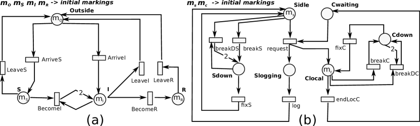
In this section we report the results obtained from the analysis of two SPN models, to show the quality and the robustness of the approximations obtained with our new approach. The first model depicted in Fig. 1(a) is inspired by the epidemiological Susceptible-Infectious-Recovered (SIR) mathematical representation of this problem originally introduced in [10] and discussed with respect to some of its variants in [4, 5]. It describes the diffusion of an epidemic on a large population, and assumes that the population members are part of three sub-populations according to their health status: (a) susceptible members (represented in the model by tokens in place S) that are not ill, but that are susceptible to the disease; (b) infected members (i.e., tokens in place I) that are subject to the disease and can spread it among susceptible members; (c) recovered members (i.e., tokens in place R) that were previously ill and are now immune. Each member of the population typically progresses from susceptible to infectious (i.e., firing of transition BecomeI) depending on the number of infected members, and from infectious to recovered (i.e., firing of transition BecomeR). Moreover, members of the population can leave the infected area (i.e., firing of transitions LeaveS, LeaveI and LeaveR) to reach the “outside world” (i.e., place Outside) and members of the outside world can enter into the infected area joining the sub-population of the susceptible (i.e., transition ArriveS) or infected members (i.e., transition ArriveI).

The second model represented in Fig. 1(b) is derived from the the PEPA representation of a Client-Server system studied in [17]. It describes an environment where servers, initially idle (tokens in place Sidle), are waiting for a client synchronization (represented by transition request). When the synchronization is completed, the client returns to its local computation (i.e., place Clocal) until the occurrence of the next synchronization (i.e., transition endLocCl), while the server executes an action log before becoming idle again (i.e., transition log). An idle server or a client in local computation may fail due to a virus infection (i.e., transitions breakS and breakC). Moreover an infected server or client can also infect other machines (i.e., transition breakDS and breakDC). Finally a server or a client recovers only when an anti-malware software discovers the virus (transitions fixS and fixC).

Figure 2: Framework architecture.

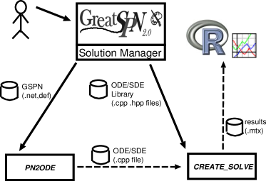
All the experiments performed on these two models have been carried on with a prototype implementation integrated in GreatSPN framework [2], which allows the generation of the ODE/SDE system from an SPN model and then the computation of its solution. The architecture of this prototype is depicted in Fig. 2 where the framework components are presented by rectangles, the component invocations by solid arrows, and the models/data exchanges by dotted arrows. More specifically, GreatSPN is used to design the SPN model and to activate the solution process, which comprises the following two steps:
1. PN2ODE generates from an SPN model a C++ file implementing the corresponding ODE/SDE system;
2. CREATE_SOLVE compiles the previously generated C++ code with the library implementing the SDE/ODE solvers, and executes it.
Finally the computed results are processed through the R framework to derive statistical information and graphics. All the results have been obtained running these programs on a 2.13 GHz Intel I7 processor with 8GB of RAM.

SIR model			Client Server model
Transition	rate (1∘ exp.)	rate (2∘ 3∘ exp.)	Transition	rate
ArriveS	0.5	1.0	log	12
ArriveI	0.5	0.01	request	1
BecomeI	1.0	1.0	endLocC	0.2
BecomeR	0.5	0.5	breakS, breakC	0.0007 0.00002
LeaveS, LeaveR	0.02	0.02	breakDS, breakDC	0.8 1.4
LeaveI	0.1	0.1	fixS, fixC	0.001 0.001

Table 1: Transition rates.

In the first set of experiments performed on the model of Fig. 1(a), we consider a situation in which the effect of barriers does not influence the correctness/quality of the solution computed by ODEs, so that we are able to properly compare the ODE approach with our new one. For this purpose, we assume that the initial marking of the model corresponds to a total of 200 people equally distributed over all the places of the model ($m_{O}=m_{S}=m_{I}=m_{R}=50$) and that the transition rates are chosen as reported in the second column of Table 1. Observe that we consider only 200 people since we want to compare the results obtained by the ODE and SDE approaches with those derived by solving the CTMC underlying the same SPN model, and because we want to stress the reliability of these methods even for cases of large, but not infinite, populations as it would instead be requested by Kurtz’s theorem for ensuring the accuracy of the approximations.

(a) Temporal behavior of the SIR members computed solving ODEs.

(b) Comparison between SDE traces (solid lines) and ODE one (dashed line)

(c) Comparison between average SDE traces (black line) and ODE one (red line)

(d) Comparison between SDEs and CTMC for infected members.

Figure 3: First SIR experiment

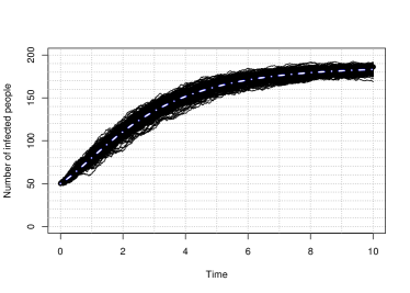
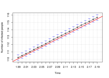
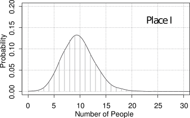
Fig. 3(a) shows the temporal behavior (i.e., between 0 to 10 time units) of the SIR members computed solving the ODE system. Similar figures obtained from the transient solution of the CTMC at different time points are not explicitly reported on these diagrams, but ensure the reliability of the method in this case. Figs. 3(b) and (c) show instead the temporal behavior of the Infected members as it is obtained by solving the SDE system with 1000 runs and Euler step equal to 0.001. In details, Fig. 3(b) plots the SDE traces (black lines) with respect to the ODE trace that is represented as the white line in the middle of the tick cloud of black lines; Fig. 3(c) reports the average SDE trace computed at specific points in time by considering the values obtained from the Euler simulations and augmented by confidence intervals that support the reliability of the method. The averages of the SDE results are represented in the diagram with the dashed black line. The results obtained with the ODEs are represented instead with a solid red line that lies next to the previous one and that is covered (in any case) by the confidence intervals obtained from the Euler Simulation. Figs. 3(b) and (c) show that the solution quality of both approaches are comparable, but it is important to highlight that the execution time for the two approaches are quite different. Indeed the solution for the ODE system requires $\sim 1$sec., while that for the SDE model is six times slower ($\sim 6$sec.). However, we can observe that this overhead in the SDE solution can be justified by the fact that the SDEs provide also the probability distribution of each sub-population at desired specific times. For instance, Fig.3(d) compares the probability distribution of Infected members at time 10 computed with GreatSPN solving the CTMC underlying the same SPN (grey dotted bars) with that computed by the SDEs (black lines) with 1000 runs. A good approximation is obtained with the SDE approach reducing the execution time by a factor of $\sim 30$ with respect to that of the CTMC solution.

The second set of experiments addresses instead a case where the presence of barriers has a negative effect on the correctness/quality of the solution computed by ODEs, while it is handled correctly by our SDE solution algorithm which is still able to reproduce the expected of the model. To stress this result, we performed this new set of experiments using the same basic model discussed before, where we changed the transition rates as reported in the third column of Table 1 and we assumed that all the population members were originally concentrated in place Outside ($m_{O}=200$ and $m_{S}=m_{I}=m_{R}=0$). With this configuration of the model, we can observe that the temporal behavior of the SIR members derived by solving the ODE system disagree with those computed solving the CTMC (see Table 2 second and third columns). This does not contradict Kurzt’s theorem since it cannot be directly applied due to the choice of these transition rate values which leads the number of Infected members to be equal to $0$ (i.e., corresponding to the lower bound of this quantity) most of the time. Instead our approach based on SDE is still able to cope with this case providing a good approximation for the CTMC solution (i.e., Table 2 second and fourth columns).

Sub-population	CTMC	ODE	SDE
S	62.636	4.367	61.906 +/-1.55
I	127.965	183.825	128.780 +/-1.48
R	4.280	4.454	4.268 +/-0.04

Table 2: Average number of members in each sub-population at time 100

In Fig.4 the probability distributions of SIR members at time 100 derived by the CTMC (grey dotted bars) are compared with those computed on the same model by SDE (black lines) with 5000 runs and step 0.01. From these graphs it is clear how our approach is still able to reproduce with a high precision these complex probability distributions reducing the memory demand (from $\sim$162MB to $\sim$1MB) and the execution time (from $\sim$600s. to $\sim$28s.).

Figure 4: Second SIR experiment: Comparison between SDEs and CTMC for SIR members

	SDE		Simulation
$|$Population$|$	Exec. Time	$E[I]_{T=100}$	Exec. Time	$E[I]_{T=100}$
200	128.78 +/-1.48	26s.	128.02+/-1.48	12s.
2,000	73.78 +/-0.19	26s.	73.51+/-0.19	155s.
20,000	735.31+/-0.62	27s.	735.03+/-0.61	20m.
200,000	7352.62+/-0.62	27s.	7352.32+/-0.62	5h.

Table 3: Comparing SDE approach with simulation varying the population size

Finally, to show how our approach scales when increasing the population, we report in Table 3. the results obtained with our method and those computed with (standard) Discrete Event Simulation. The first column of Table 3 reports the population size, the second and third show the average number of infected members at time 100 computed with the SDE approach and the execution time needed for its computation; similarly, the last two columns contain the same information referred to the Discrete Event Simulation. From these results it is clear how our approach is able to obtain a speed-up with respect to the Discrete Event Simulation requiring the same used memory. Obviously this speed-up depends on the characteristic of the model and increases/decreases proportionally to the time spent by the quantities of interest on their boundaries. Indeed, as explained in Sec.3, every time that a quantity of interest reaches one of its bounds, our approach uses a classical Discrete Event Simulation to derive its next evolution step.

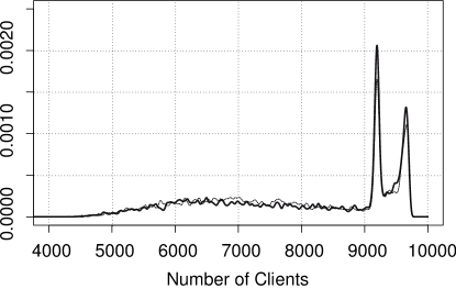
The last set of experiments is related to the Client Server system and shows how the SDE approach deals with models exhibiting multi-modal behavior. Indeed, choosing the transition rates as reported in the last two columns of Table 1 and an initial marking with 120 idle servers and 10,000 clients in local computation, we can observe that the probability distribution of tokens in place Cwaiting at time 18, computed thought Discrete Event Simulation, has a multi-modal shape (see Fig.5 dashed light line). In particular, the first mode corresponds to the situation where most of the clients failed, the second one to the situation where only few servers are down and few clients are failed, and the last mode to the situation where most of the servers are down and only few clients are failed. Comparing this dashed line with the black solid line plotting the same measure computed by the SDE approach, we can observe that a good level of approximation is attained by such an approach reducing the computation time by a factor of $\sim 13$. Indeed, the two lines are often difficult to distinguish (thus showing the good level of agreement between the two methods) thus identifying the modes (picks) of the distributions in a satisfactory manner, even if the absolute values of the two lines are not perfectly matched in these cases.

Figure 5: First client server experiment: comparison between SDEs and Discrete Event Simulation for the distribution of tokens in place Cwaiting at time 18

5 Conclusion

In this paper we considered approximations of SPNs. We identified a class of SPNs for which the underlying stochastic process is a density dependent CTMC. Consequently, it is possible to apply to these SPNs both a deterministic approximation based on ODEs and a diffusion approximation based on SDEs, both being introduced by Kurtz. The diffusion approximation, as presented in its original form, is defined only up to the first exit from an open set. Since in many applications barriers are important, we extended the diffusion approximation by jumps that take into account the behavior of the process on the barriers. We showed by numerical examples that the resulting jump diffusion approximation provides precise information about the distribution of the involved quantities and outperforms the deterministic approach when the original process is with significant variability or it involves distributions whose mean value does not carry much information. Future work will investigate the numerical aspects of the prototype implementation used for the experiments and the possibility of applying these idea to the analysis of hybrid models.

Acknowledgments. We gratefully acknowledge the anonymous referees for their useful suggestions that helped improving the final version of the paper. This work has been supported in part by project “AMALFI ” sponsored by Universitå di Torino and Compagnia di San Paolo.

References

- [1] Ajmone Marsan, M., Balbo, G., Conte, G., Donatelli, S., Franceschinis, G.: Modelling with Generalized Stochastic Petri Nets. J. Wiley, New York, NY, USA (1995)
- [2] Babar, J., Beccuti, M., Donatelli, S., Miner, A.S.: Greatspn enhanced with decision diagram data structures. In: Proceedings of Applications and Theory of Petri Nets, 31st Int. Conference, Braga, Portugal, June 21-25,. pp. 308–317. IEEE Computer Society (June 2010)
- [3] Balbo, G.: Introduction to Stochastic Petri Nets. In: Brinksma, E., Hermanns, H., Katoen, J.P. (eds.) Formal Methods and Performance Analysis, LNCS Vol. 2090, pp. 84–155. Springer-Verlag, Berlin, Germany (May 2001)
- [4] Beccuti, M., Franceschinis, G.: Efficient simulation of stochastic well-formed nets through symmetry exploitation. In: Proceedings of the Winter Simulation Conference. pp. 296:1–296:13. WSC ’12, IEEE Computer Society (Dec 2012)
- [5] Beccuti, M., Fornari, C., Franceschinis, G., Halawani, S.M., Ba-Rukab, O., Ahmad, A.R., Balbo, G.: From symmetric nets to differential equations exploiting model symmetries. The Computer Journal (2013)
- [6] Brémaud, P.: Markov chains, Texts in Applied Mathematics, vol. 31. Springer-Verlag, New York (1999), gibbs fields, Monte Carlo simulation, and queues
- [7] Fishman, G.S.: Principles of Discrete Event Simulation. John Wiley & Sons, Inc., New York, NY, USA (1978)
- [8] Gaeta, R.: Efficient Discrete-Event Simulation of Colored Petri Nets. IEEE Transactions on Software Engineering 22(9), 629–639 (1996)
- [9] Gillespie, D.T.: The chemical langevin equation. J. Chem. Phys. 113, 297 (2000)
- [10] Kermack, W., McKendrick, A.: A contribution to the mathematical theory of epidemics. Proceedings of the Royal Society of London. Series A 115(772), 700–721 (Aug 1927)
- [11] Klebaner, F.C.: Introduction to stochastic calculus with applications. Imperial College Press, London, third edn. (2012)
- [12] Kloeden, P.E., Platen, E.: Numerical solution of stochastic differential equations, vol. 23. Springer (1992)
- [13] Kurtz, T.G.: Solutions of ordinary differential equations as limits of pure jump Markov processes. Journal of Applied Probability 1(7), 49–58 (1970)
- [14] Kurtz, T.G.: Limit theorems and diffusion approximations for density dependent markov chains. In: Stochastic Systems: Modeling, Identification and Optimization, I, pp. 67–78. Springer (1976)
- [15] Kurtz, T.G.: Strong approximation theorems for density dependent markov chains. Stochastic Processes and Their Applications 6(3), 223–240 (1978)
- [16] Molloy, M.K.: Performance analysis using stochastic Petri Nets. IEEE Transactions on Computers 31(9), 913–917 (1982)
- [17] Pourranjbar, A., Hillston, J., Bortolussi, L.: Don’t just go with the flow: Cautionary tales of fluid flow approximation. In: Tribastone, M., Gilmore, S. (eds.) EPEW 2012, and UKPEW 2012. Lecture Notes in Computer Science, vol. 7587, p. 156–171. Springer (2012)
- [18] Tribastone, M.: Scalable differential analysis of large process algebra models. In: 7th Int. Conference on the Quantitative Evaluation of Systems. p. 307. IEEE Computer Society, Williamsburg, Virginia, USA (sept 2010)
- [19] Tribastone, M., Gilmore, S., Hillston, J.: Scalable differential analysis of process algebra models. IEEE Trans. Software Eng. 38(1), 205–219 (2012)