Optimal Power Control for Analog Bidirectional Relaying with Long-Term Relay Power Constraint

Zoran Hadzi-Velkov1, Nikola Zlatanov2, and Robert Schober3 1Faculty of Electrical Engineering and Information Technologies, Ss. Cyril and Methodius University, Skopje, Macedonia 3Department of Electrical, Electronics and Communications Engineering, University of Erlangen-Nuremberg, Germany 2Department of Electrical and Computer Engineering, University of British Columbia, Vancouver, Canada
Abstract

Wireless systems that carry delay-sensitive information (such as speech and/or video signals) typically transmit with fixed data rates, but may occasionally suffer from transmission outages caused by the random nature of the fading channels. If the transmitter has instantaneous channel state information (CSI) available, it can compensate for a significant portion of these outages by utilizing power allocation. In a conventional dual-hop bidirectional amplify-and-forward (AF) relaying system, the relay already has instantaneous CSI of both links available, as this is required for relay gain adjustment. We therefore develop an optimal power allocation strategy for the relay, which adjusts its instantaneous output power to the minimum level required to avoid outages, but only if the required output power is below some cutoff level; otherwise, the relay is silent in order to conserve power and prolong its lifetime. The proposed scheme is proven to minimize the system outage probability, subject to an average power constraint at the relay and fixed output powers at the end nodes.

โ€ โ€ footnotetext: This work has been supported by the Alexander von Humboldt fellowship program for experienced researchers

I Introduction

Bidirectional (two-way) relaying has higher bandwidth efficiency compared to unidirectional relaying [1]-[3], and it is also a more suitable option for applications where the end nodes intend to exchange information (e.g., in interactive applications). The amplify-and-forward (AF) version of bidirectional relaying, often referred to as the analog network coding [3], has recently been extensively studied [4]-[10]. In this paper, we consider bidirectional analog network coding with fixed information rates, which is suitable for delay-sensitive applications, such as bidirectional interactive speech and/or video communication. Fixed-rate communication systems are usually characterized by the capacity outage probability (OP), which is a relevant performance measure in quasi-static (i.e., slowly fading) channels. In these systems, each transmitted codeword is affected by only one channel realization.

Papers [4], [5], and [6] focus on the OP analysis of dual-hop bidirectional AF systems. However, [4] and [5] assume that the end nodes and the relay transmit with fixed powers, although they have instantaneous channel state information (CSI) available. In particular, for each channel realization, the relay needs CSI to set the amplification gain factor, whereas the end nodes need CSI to cancel out self-interference and to decode the desired codeword. The available CSI in fixed-rate bidirectional relaying systems can be used for optimal power allocation at the end nodes and the relay. Papers [6]-[9] develop power allocation schemes that optimize different system objectives; [6] minimizes the OP of either one of the two traffic flows, [8] proposes a power allocation that balances the individual outage probabilities of the two end nodes, [7] maximizes the instantaneous sum rate of bidirectional AF systems, and [9] minimizes the total consumed energy such that the OPs of both traffic flows are maintained below some predefined values. However, the power allocations in these papers are subject to short-term power constraints, which limits the codeword power in each channel realization.

On the other hand, it is also possible to adopt average (long-term) power constraints so as to limit the average power of all codewords over all channel realizations [12]. For point-to-point channels, such power adaptation is known as truncated channel inversion and has been introduced in [13]. For unidirectional relaying, optimal power allocation for source and relay has been studied for both conventional amplify-and-forward [10] and decode-and-forward (DF) [11] relaying systems under various average power constraints. Optimal power allocation has been shown to introduce significant performance improvement relative to constant power transmission [10]-[13]. However, the literature does not offer similar results for bidirectional relaying with long-term power constraints.

In this work, we derive power control strategies for the relay in bidirectional dual-hop AF relaying systems. For predefined constant rates in both directions, the proposed power allocation achieves minimization of the system OP assuming an average power constraint at the relay. The end nodes are assumed to be simple nodes, equipped with cheap power amplifiers, and therefore are unable to support the high peak-to-average power ratios at their output, required for channel inversion. Thus, the end nodes transmit with fixed powers.

The relay applies the proposed optimal power control strategy based on the already available knowledge of the channel coefficients of both links. Intuitively, it is not necessary for the relay to transmit at its maximum available power in each transmission cycle, but to transmit with the minimum power required to avoid outages, or sometimes even be silent when outages are unavoidable, thus conserving power. In other words, we allow outages to occur in cases of deep fades, but for the rest of the time we ensure successful transmissions at the predefined constant transmission rate.

II System and channel model

The considered bidirectional relaying system comprises two end-nodes ($S_{1}$ and $S_{2}$) and a half-duplex AF relay $R$. The bidirectional communication consists of two parallel unidirectional communication sessions, $S_{1}\rightarrow S_{2}$ and $S_{2}\rightarrow S_{1}$. Each communication session is realized at a fixed information rate, $R_{01}$ and $R_{02}$, respectively. The OP for this system is defined as the probability that at least one (or both) of the communications sessions is in outage.

The complex coefficients of the $S_{1}-R$ and $S_{2}-R$ channels are denoted by $\alpha$ and $\beta$, respectively, whereas their respective squared amplitudes are $x=|\alpha|^{2}$ and $y=|\beta|^{2}$ with average values $\Omega_{X}$ and $\Omega_{Y}$. We assume that the $R-S_{1}$ channel is reciprocal to the $S_{1}-R$ channel, and the $R-S_{2}$ channel is reciprocal to the $S_{2}-R$ channel. We adopt the Rayleigh block fading model, which means that the values of $\alpha$ and $\beta$ are constant for each transmission cycle, but change from one transmission cycle to the next. In each transmission cycle, the pair $\left(x,y\right)$ denotes the channel state, where both $x$ and $y$ follow an exponential probability density function (PDF). The received signals at the end nodes and the relay are corrupted by additive white Gaussian noise (AWGN) with zero mean and unit variance.

We assume a two-phase transmission cycle consisting of the mutiple access phase and the broadcast phase. In two-phase relaying, bidirectional communication can be realized only via the relayed link $S_{1}-R-S_{2}$. In the first phase, $S_{1}$ and $S_{2}$ simultaneously transmit their codewords s1โ€‹(t)subscript๐‘ 1๐‘กs_{1}(t) and s2โ€‹(t)subscript๐‘ 2๐‘กs_{2}\left(t\right) with respective information rates $R_{01}$ and $R_{02}$ and respective fixed output powers $P_{S1}$ and $P_{S2}$. The AF relay receives the composite signal and amplifies it by applying the following gain:

$$G^{2}=\frac{P_{R}\left(x,y\right)}{P_{S1}x+P_{S2}y+1}\text{,}$$ (1)

where $P_{R}\left(x,y\right)$ is the relay output power, adjusted according to the channel state $\left(x,y\right)$. The relay is assumed to know $x$ and $y$.

In the second phase, the relay broadcasts the composite signal and the end nodes receive it. Node $S_{1}$ is assumed to know the products $G\alpha\beta$ and $G\alpha^{2}$, whereas node $S_{2}$ is assumed to know the products $G\alpha\beta$ and $G\beta^{2}$. Using the available CSI, each end node โ€œsubtractsโ€ its own signal from the received one, and then attempts decoding of the faded and noisy version of the desired signal that originates from the other end node. The desired signal-to-noise ratio (SNR) at $S_{2}$ is thus given by

$$\gamma_{2}=\frac{P_{S1}x\text{ }P_{R}y}{P_{S1}x+\left(P_{S2}+P_{R}\right)y+1}\text{,}$$ (2)

whereas the SNR at $S_{1}$ is given by

ฮณ1=PSโ€‹2โ€‹xโ€‹ย โ€‹PRโ€‹y(PSโ€‹1+PR)โ€‹x+PSโ€‹2โ€‹y+1โ€‹.ย subscript๐›พ1subscript๐‘ƒ๐‘†2๐‘ฅย subscript๐‘ƒ๐‘…๐‘ฆsubscript๐‘ƒ๐‘†1subscript๐‘ƒ๐‘…๐‘ฅsubscript๐‘ƒ๐‘†2๐‘ฆ1.ย \gamma_{1}=\frac{P_{S2}x\text{ }P_{R}y}{\left(P_{S1}+P_{R}\right)x+P_{S2}y+1}\text{. } (3)

Based on (2) and (3), the relaying system can support $S_{1}$โ€™s transmission rate, $R_{01}$, if the instantaneous capacity of the end-to-end channel $S_{1}\rightarrow R\rightarrow S_{2}$ exceeds this rate such that $\frac{1}{2}\log_{2}\left(1+\gamma_{2}\right)\geq R_{01}$, where the pre-log factor $1/2$ is due to the two-phase transmission cycle, or equivalently $\gamma_{2}\geq\delta_{1}$, where $\delta_{1}=2^{2R_{01}}-1$. Similarly, the relaying system can support $S_{2}$โ€™s transmission rate, $R_{02}$, if the instantaneous capacity of the end-to-end channel $S_{2}\rightarrow R\rightarrow S_{1}$ exceeds this rate such that $\frac{1}{2}\log_{2}\left(1+\gamma_{1}\right)\geq R_{02}$, or equivalently $\gamma_{1}\geq\delta_{2}$, where $\delta_{2}=2^{2R_{02}}-1$. The system OP is therefore determined as

$\displaystyle P_{out}=\Pr\left\{\frac{1}{2}\log_{2}\left(1+\gamma_{2}\right)<R_{01}\text{ OR }\frac{1}{2}\log_{2}\left(1+\gamma_{1}\right)<R_{02}\right\}$
=1โˆ’Prโก{ฮณ2โ‰ฅฮด1โ€‹ย ANDย โ€‹ฮณ1โ‰ฅฮด2}โ€‹,ย absent1Prsubscript๐›พ2subscript๐›ฟ1ย ANDย subscript๐›พ1subscript๐›ฟ2,ย =1-\Pr\left\{\gamma_{2}\geq\delta_{1}\text{ AND }\gamma_{1}\geq\delta_{2}\right\}\text{, } (4)

where $\gamma_{2}$ and $\gamma_{1}$ are given by (2) and (3), respectively.

III Outage Minimization

We now present the optimal power allocation (OPA) strategy at the relay, $P_{R}^{\ast}\left(x,y\right)$, that minimize the system OP, subject to a (long-term) average power constraint at the relay, $P_{avg}$, and fixed output powers at the end nodes, $P_{S1}$ and $P_{S2}$. The OPA is specified in the following theorem.

Theorem 1

For the system OP defined as in (4), the solution of the optimization problem

$$\underset{P_{R}\left(x,y\right)}{\text{minimize}}\text{ }P_{out}$$
$$\text{subject to \ \ \ }E_{XY}\left[P_{R}\left(x,y\right)\right]\leq P_{avg}$$ (5)

where $E_{XY}\left[\cdot\right]$ denotes expectation with respect to random variables $X$ and $Y$, is given by

PRโˆ—โ€‹(x,y,ฯ)={PR,sโ€‹tโ€‹(x,y),ย ifย โ€‹PR,sโ€‹tโ€‹(x,y)โ‰คฯ0,ย ifย โ€‹PR,sโ€‹tโ€‹(x,y)>ฯsuperscriptsubscript๐‘ƒ๐‘…โˆ—๐‘ฅ๐‘ฆ๐œŒcasessubscript๐‘ƒ๐‘…๐‘ ๐‘ก๐‘ฅ๐‘ฆย ifย subscript๐‘ƒ๐‘…๐‘ ๐‘ก๐‘ฅ๐‘ฆ๐œŒ0ย ifย subscript๐‘ƒ๐‘…๐‘ ๐‘ก๐‘ฅ๐‘ฆ๐œŒP_{R}^{\ast}\left(x,y,\rho\right)=\left\{\begin{array}[]{c}P_{R,st}\left(x,y\right),\text{ \ \ if }P_{R,st}\left(x,y\right)\leq\rho\\ 0,\text{ \ \ \ \ \ \ \ \ \ \ \ \ \ \ \ if }P_{R,st}\left(x,y\right)>\rho\end{array}\right. (6)

where PR,sโ€‹tโ€‹(x,y)subscript๐‘ƒ๐‘…๐‘ ๐‘ก๐‘ฅ๐‘ฆP_{R,st}\left(x,y\right) is the minimum short-term relay power that maintains zero OP, and $\rho$ is the cutoff threshold determined from

Paโ€‹vโ€‹g=EXโ€‹Yโ€‹[PR,sโ€‹tโ€‹(x,y)โ€‹ย |PR,sโ€‹tโ€‹(x,y)โ‰คฯ]โ€‹ย .subscript๐‘ƒ๐‘Ž๐‘ฃ๐‘”subscript๐ธ๐‘‹๐‘Œdelimited-[]conditionalsubscript๐‘ƒ๐‘…๐‘ ๐‘ก๐‘ฅ๐‘ฆย subscript๐‘ƒ๐‘…๐‘ ๐‘ก๐‘ฅ๐‘ฆ๐œŒย .P_{avg}=E_{XY}\left[P_{R,st}\left(x,y\right)\text{ }|P_{R,st}\left(x,y\right)\leq\rho\right]\text{ .} (7)
Proof:

The proof is presented in the Appendix. โˆŽ

Intuitively, the solution in (6) resembles the truncated channel inversion in point-to-point communication links [13]. The minimum possible short-term power PR,sโ€‹tโ€‹(x,y)subscript๐‘ƒ๐‘…๐‘ ๐‘ก๐‘ฅ๐‘ฆP_{R,st}\left(x,y\right) prevents system outage events to the greatest possible extent, such that the average relay output power is below the predefined value $P_{avg}$. The cutoff threshold $\rho$ assures that the long-term average power constraint is satisfied, such that the relay is silent if PR,sโ€‹tโ€‹(x,y)subscript๐‘ƒ๐‘…๐‘ ๐‘ก๐‘ฅ๐‘ฆP_{R,st}\left(x,y\right) exceeds $\rho$. In the following subsections, we determine PR,sโ€‹tโ€‹(x,y)subscript๐‘ƒ๐‘…๐‘ ๐‘ก๐‘ฅ๐‘ฆP_{R,st}\left(x,y\right) and $\rho$.

III-A Minimum Short-term Power Required for Zero Outage

The power control scheme that maintains zero outage probability and also minimizes the relay output power is determined according to the following theorem.

Theorem 2

The solution of optimization problem

$$\text{$\underset{P_{R}\left(x,y\right)}{\text{minimize}}$ }P_{R}\left(x,y\right)$$
$\displaystyle\text{subject to \ \ }\frac{1}{2}\log_{2}\left(1+\gamma_{2}\right)$ $\displaystyle\geq$ $\displaystyle R_{01}$
$\displaystyle\frac{1}{2}\log{}_{2}\left(1+\gamma_{1}\right)$ $\displaystyle\geq$ $\displaystyle R_{02}$ (8)

is given by

PR,sโ€‹tโ€‹(x,y)={maxโก{ฮด1โ€‹(1+PSโ€‹1โ€‹x+PSโ€‹2โ€‹y)yโ€‹(PSโ€‹1โ€‹xโˆ’ฮด1),ฮด2โ€‹(1+PSโ€‹1โ€‹x+PSโ€‹2โ€‹y)xโ€‹(PSโ€‹2โ€‹yโˆ’ฮด2)}โ€‹,ย ifย โ€‹xโ‰ฅฮด1PSโ€‹1โ€‹ย andย โ€‹yโ‰ฅฮด2PSโ€‹20,ย otherwise.subscript๐‘ƒ๐‘…๐‘ ๐‘ก๐‘ฅ๐‘ฆcasessubscript๐›ฟ11subscript๐‘ƒ๐‘†1๐‘ฅsubscript๐‘ƒ๐‘†2๐‘ฆ๐‘ฆsubscript๐‘ƒ๐‘†1๐‘ฅsubscript๐›ฟ1subscript๐›ฟ21subscript๐‘ƒ๐‘†1๐‘ฅsubscript๐‘ƒ๐‘†2๐‘ฆ๐‘ฅsubscript๐‘ƒ๐‘†2๐‘ฆsubscript๐›ฟ2,ย ifย ๐‘ฅsubscript๐›ฟ1subscript๐‘ƒ๐‘†1ย andย ๐‘ฆsubscript๐›ฟ2subscript๐‘ƒ๐‘†2missing-subexpression0ย otherwiseP_{R,st}\left(x,y\right)=\left\{\begin{array}[]{c}\max\left\{\frac{\delta_{1}\left(1+P_{S1}x+P_{S2}y\right)}{y\left(P_{S1}x-\delta_{1}\right)},\frac{\delta_{2}\left(1+P_{S1}x+P_{S2}y\right)}{x\left(P_{S2}y-\delta_{2}\right)}\right\}\text{, }\\ \text{if }x\geq\frac{\delta_{1}}{P_{S1}}\text{ and }y\geq\frac{\delta_{2}}{P_{S2}}\\ \\ 0,\text{ otherwise}\end{array}\right.. (9)
Proof:

Optimization problem (8) is a standard linear programming (LP) problem, whose solution is feasible because the intersection of the constraints in (8) is a non-empty set, and the solution lies at the boundary of the intersection. Considering (2), the first constraint in (8) is satisfied if the output powers of the relay and the end node $S_{1}$ satisfy the following conditions:

$$P_{R}\geq\frac{\delta_{1}\left(1+P_{S1}x+P_{S2}y\right)}{y\left(P_{S1}x-\delta_{1}\right)}\text{ \ and \ }P_{S1}x-\delta_{1}\geq 0\text{.}$$ (10)

The second constraint in (8) is satisfied if the output powers of the relay and the end node $S_{2}$ satisfy the following conditions:

$$P_{R}\geq\frac{\delta_{2}\left(1+P_{S1}x+P_{S2}y\right)}{x\left(P_{S2}y-\delta_{2}\right)}\text{ \ and \ }P_{S2}y-\delta_{2}\geq 0\text{.}$$ (11)

Then, the intersection of (10) and (11) is given by (9). If either one of the conditions $P_{S1}x-\delta_{1}\geq 0$ and $P_{S2}y-\delta_{2}\geq 0$ is not satisfied, then the intersection is an empty set, which practically means that the relay should be silent, i.e., PR,sโ€‹tโ€‹(x,y)=0subscript๐‘ƒ๐‘…๐‘ ๐‘ก๐‘ฅ๐‘ฆ0P_{R,st}\left(x,y\right)=0. In this case, an outage event is unavoidable regardless of the available short-term power at the relay. This concludes the proof. โˆŽ

Refer to caption
Figure 1: Non-outage region $\mathcal{M}=\mathcal{M}_{1}\cup\mathcal{M}_{2}$.

III-B Average Relay Output Power and Cutoff Threshold $\rho$

The combination of (6) and (9) is the general analytical solution to the considered outage minimization problem (5). In order to be able to obtain $\rho$ analytically, it is necessary to derive an analytical expression for the average relay output power, PยฏR=EXโ€‹Yโ€‹[PR,sโ€‹tโ€‹(x,y)โ€‹ย |PR,sโ€‹tโ€‹(x,y)โ‰คฯ]subscriptยฏ๐‘ƒ๐‘…subscript๐ธ๐‘‹๐‘Œdelimited-[]conditionalsubscript๐‘ƒ๐‘…๐‘ ๐‘ก๐‘ฅ๐‘ฆย subscript๐‘ƒ๐‘…๐‘ ๐‘ก๐‘ฅ๐‘ฆ๐œŒ\overline{P}_{R}=E_{XY}\left[P_{R,st}\left(x,y\right)\text{ }|P_{R,st}\left(x,y\right)\leq\rho\right], where PR,sโ€‹tโ€‹(x,y)subscript๐‘ƒ๐‘…๐‘ ๐‘ก๐‘ฅ๐‘ฆP_{R,st}\left(x,y\right) is given by (9). Although possible, arriving at a general analytic expression for $\overline{P}_{R}$ for arbitrary fixed output powers at the end nodes and arbitrary rates requires lengthy derivations due to the complicated system non-outage regions. Thus, due to the space restriction, here we focus on the following special case:

$$\frac{P_{S1}}{\delta_{1}}=\frac{P_{S2}}{\delta_{2}}\text{.}$$ (12)

Assuming (12), the system non-outage region โ„ณ={(x,y)|PSโ€‹1โ€‹xโ‰ฅฮด1,PSโ€‹2โ€‹yโ‰ฅฮด2,PR,sโ€‹tโ€‹(x,y)โ‰คฯ}โ„ณconditional-set๐‘ฅ๐‘ฆformulae-sequencesubscript๐‘ƒ๐‘†1๐‘ฅsubscript๐›ฟ1formulae-sequencesubscript๐‘ƒ๐‘†2๐‘ฆsubscript๐›ฟ2subscript๐‘ƒ๐‘…๐‘ ๐‘ก๐‘ฅ๐‘ฆ๐œŒ\mathcal{M}=\left\{\left(x,y\right)\left|P_{S1}x\geq\delta_{1},P_{S2}y\geq\delta_{2},P_{R,st}\left(x,y\right)\leq\rho\right.\right\} is divided into two non-overlapping regions, $\mathcal{M}=\mathcal{M}_{1}\cup\mathcal{M}_{2}$, such that

$$\mathcal{M}_{1}:\frac{\delta_{1}\left[1+\left(P_{S2}+\rho\right)y\right]}{P_{S1}\left(\rho y-\delta_{1}\right)}\leq x\leq y\text{ and }y\geq\lambda\left(\rho\right)$$ (13)
$$\mathcal{M}_{2}:\frac{\delta_{2}\left[1+\left(P_{S1}+\rho\right)x\right]}{P_{S2}\left(\rho x-\delta_{2}\right)}\leq y\leq x\text{ and }x\geq\lambda\left(\rho\right)$$ (14)

where

$\displaystyle\lambda\left(\rho\right)$ $\displaystyle=$ $\displaystyle\frac{\delta_{2}\left(P_{S1}+P_{S2}+\rho\right)}{2P_{S2}\rho}$ (15)
$\displaystyle\times\left(1+\sqrt{1+\frac{4P_{S2}\rho}{\delta_{2}\left(P_{S1}+P_{S2}+\rho\right)^{2}}}\right)\text{.}$

Note that $\lambda\left(\rho\right)>P_{S1}/\delta_{1}$. Fig. 1 graphically illustrates the non-outage regions $\mathcal{M}_{1}$ and $\mathcal{M}_{2}$. Considering (13)-(15), the average output power of the power control scheme (9) is determined as

$\displaystyle\overline{P}_{R}$ $\displaystyle=$ EXโ€‹Yโ€‹[PR,sโ€‹tโ€‹(x,y)โ€‹ย |PR,sโ€‹tโ€‹(x,y)โ‰คฯ]subscript๐ธ๐‘‹๐‘Œdelimited-[]conditionalsubscript๐‘ƒ๐‘…๐‘ ๐‘ก๐‘ฅ๐‘ฆย subscript๐‘ƒ๐‘…๐‘ ๐‘ก๐‘ฅ๐‘ฆ๐œŒ\displaystyle E_{XY}\left[P_{R,st}\left(x,y\right)\text{ }|P_{R,st}\left(x,y\right)\leq\rho\right] (16)
$\displaystyle=$ $\displaystyle\int_{\lambda\left(\rho\right)}^{\infty}\int_{\frac{\delta_{1}\left[1+\left(P_{S2}+\rho\right)y\right]}{P_{S1}\left(\rho y-\delta_{1}\right)}}^{y}dxdyf_{X}\left(x\right)f_{Y}\left(y\right)$
$\displaystyle\times\frac{\delta_{1}\left(1+P_{S1}x+P_{S2}y\right)}{y\left(P_{S1}x-\delta_{1}\right)}$
$\displaystyle+\int_{\lambda\left(\rho\right)}^{\infty}\int_{\frac{\delta_{2}\left[1+\left(P_{S1}+\rho\right)x\right]}{P_{S2}\left(\rho x-\delta_{2}\right)}}^{x}dydxf_{X}\left(x\right)f_{Y}\left(y\right)$
$\displaystyle\times\frac{\delta_{2}\left(1+P_{S1}x+P_{S2}y\right)}{x\left(P_{S2}y-\delta_{2}\right)}\text{.}$

The inner integral in (16) can be solved in closed-form using the exponential integral function $E_{1}\left(\cdot\right)$ [14], which is omitted here due to space limitation. Therefore, (16) can be expressed as a single integral, which depends on the cutoff threshold $\rho$. Thus, $\rho$ can be determined numerically for a given $P_{avg}$.

III-C Optimum Power Allocation and Minimum Outage Probability

Exploiting (13)-(15), we combine (6) and (9) to arrive at the final OPA expression

$$P_{R}^{\ast}\left(x,y,\rho\right)=\qquad\qquad\qquad\qquad\qquad\qquad\qquad\qquad\,$$ (17)
$\displaystyle\left\{\begin{array}[]{c}\frac{\delta_{1}\left(1+P_{S1}x+P_{S2}y\right)}{y\left(P_{S1}x-\delta_{1}\right)}\text{, if }\frac{\delta_{1}\left[1+\left(P_{S2}+\rho\right)y\right]}{P_{S1}\left(\rho y-\delta_{1}\right)}\leq x\leq y\text{ and }y\geq\lambda\left(\rho\right)\\ \frac{\delta_{2}\left(1+P_{S1}x+P_{S2}y\right)}{x\left(P_{S2}y-\delta_{2}\right)}\text{, if }\frac{\delta_{2}\left[1+\left(P_{S1}+\rho\right)x\right]}{P_{S2}\left(\rho x-\delta_{2}\right)}\leq y\leq x\text{ and }x\geq\lambda\left(\rho\right)\\ 0\qquad\qquad\qquad\qquad,\text{ otherwise}\end{array}\right.$

Assuming power allocation (17), the system OPย (4) is determined as $P_{out}=1-\Pr\left\{(x,y)\in\mathcal{M}\right\}$, i.e.,

$\displaystyle P_{out}\left(\rho\right)$ $\displaystyle=$ $\displaystyle 1-\int_{\lambda\left(\rho\right)}^{\infty}\int_{\frac{\delta_{1}\left[1+\left(P_{S2}+\rho\right)y\right]}{P_{S1}\left(\rho y-\delta_{1}\right)}}^{y}f_{X}\left(x\right)f_{Y}\left(y\right)dxdy\qquad\,$
$\displaystyle-\int_{\lambda\left(\rho\right)}^{\infty}\int_{\frac{\delta_{2}\left[1+\left(P_{S1}+\rho\right)x\right]}{P_{S2}\left(\rho x-\delta_{2}\right)}}^{x}f_{X}\left(x\right)f_{Y}\left(y\right)dydx\qquad\qquad\qquad$
$\displaystyle=1+e^{-\lambda\left(\frac{1}{\Omega_{X}}+\frac{1}{\Omega_{Y}}\right)}\qquad\qquad\qquad\qquad\qquad\qquad\qquad\quad$
$\displaystyle-\frac{1}{\Omega_{Y}}\int_{\lambda}^{\infty}\exp\left[-\left(\frac{z}{\Omega_{Y}}+\frac{\delta_{1}}{\Omega_{X}P_{S1}}\frac{1+\left(P_{S2}+\rho\right)}{\rho z-\delta_{1}}\right)\right]dz$
$\displaystyle-\frac{1}{\Omega_{X}}\int_{\lambda}^{\infty}\exp\left[-\left(\frac{z}{\Omega_{X}}+\frac{\delta_{2}}{\Omega_{Y}P_{S2}}\frac{1+\left(P_{S1}+\rho\right)}{\rho z-\delta_{2}}\right)\right]dz\text{.}$ (19)

For a given $P_{avg}$, the cutoff threshold $\rho$ is determined from (16), and (19) leads to the minimum OP of the considered bidirectional relaying system. However, note that (19) is also the system OP for a relay with constant output power set as $P_{R}\left(x,y,\rho\right)=\rho$. For $\rho\rightarrow\infty$ (i.e., $P_{avg}\rightarrow\infty$), (19) attains its minimum value given by

Poโ€‹uโ€‹tmin=1โˆ’eโˆ’ฮด1PSโ€‹1โ€‹(1ฮฉX+1ฮฉY)โ€‹.ย superscriptsubscript๐‘ƒ๐‘œ๐‘ข๐‘ก1superscript๐‘’subscript๐›ฟ1subscript๐‘ƒ๐‘†11subscriptฮฉ๐‘‹1subscriptฮฉ๐‘Œ.ย P_{out}^{\min}=1-e^{-\frac{\delta_{1}}{P_{S1}}\left(\frac{1}{\Omega_{X}}+\frac{1}{\Omega_{Y}}\right)}\text{. } (20)

Namely, regardless of the available relay power, the outages are imminent if the channel between the originating end node and the relay cannot support the desired rate. We again note that (16)-(20) are valid under assumption (12).

III-D Minimization of Average Relay Power

The following theorem determines the solution of the dual optimization problem of (5), which minimizes the average relay output power subject to some target system OP, $P_{out}^{\max}$.

Theorem 3

For system OP $P_{out}$ defined as per (4), the solution of optimization problem

$$\text{$\underset{P_{R}\left(x,y\right)}{\text{minimize}}$ \ }E_{XY}\left[P_{R}\left(x,y\right)\right]$$
$$\text{subject to \ \ }P_{out}\leq P_{out}^{\text{target}}\text{,}$$ (21)

is given by

PRโˆ—โˆ—โ€‹(x,y,ฮผ)={PR,sโ€‹tโ€‹(x,y),ย ifย โ€‹PR,sโ€‹tโ€‹(x,y)โ‰คฮผ0,ย ifย โ€‹PR,sโ€‹tโ€‹(x,y)>ฮผ,superscriptsubscript๐‘ƒ๐‘…โˆ—absentโˆ—๐‘ฅ๐‘ฆ๐œ‡casessubscript๐‘ƒ๐‘…๐‘ ๐‘ก๐‘ฅ๐‘ฆย ifย subscript๐‘ƒ๐‘…๐‘ ๐‘ก๐‘ฅ๐‘ฆ๐œ‡0ย ifย subscript๐‘ƒ๐‘…๐‘ ๐‘ก๐‘ฅ๐‘ฆ๐œ‡P_{R}^{\ast\ast}\left(x,y,\mu\right)=\left\{\begin{array}[]{c}P_{R,st}\left(x,y\right),\text{ \ \ if }P_{R,st}\left(x,y\right)\leq\mu\\ 0,\text{ \ \ \ \ \ \ \ \ \ \ \ \ \ \ \ if }P_{R,st}\left(x,y\right)>\mu\end{array}\right., (22)

where PR,sโ€‹tโ€‹(x,y)subscript๐‘ƒ๐‘…๐‘ ๐‘ก๐‘ฅ๐‘ฆP_{R,st}\left(x,y\right) is given by (9), whereas the cutoff threshold $\mu$ satisfies

$$P_{out}\left(\mu\right)=P_{out}^{\text{target}}\text{,}$$ (23)

where $P_{out}\left(\mu\right)$ given by (19).

Proof:

A sketch of the proof is provided in Appendix B. โˆŽ

Refer to caption
Figure 2: Outage performance improvement due to power allocation.
Refer to caption
Figure 3: Power savings at the end nodes and the relay.

IV Numerical Examples

We illustrate the performance gains of the proposed OPA for the considered three-node AF relaying system under two different scenarios. For both scenarios, the rates are fixed to $R_{01}=R_{02}=1/2$.

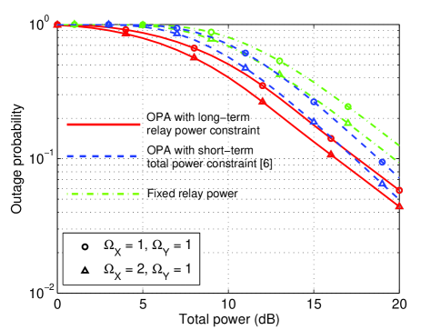
Scenario 1: We compare the system OP of the proposed OPA with: (i) fixed power allocation (FPA), and (ii) OPA with short-term total power constraint as derived in [6], denoted as short-term OPA. Note, for each channel realization, the short-term OPA optimally allocates the same amount of the total available power to the relay and the two end nodes. For a given total available power $P_{T}$, the system using the proposed OPA employs $P_{S1}=P_{S2}=P_{avg}=P_{T}/3$; the system using FPA employs $P_{S1}=P_{S2}=P_{R}=P_{T}/3$; the system using the short-term OPA employs [6, Es. (15)-(17)]: $P_{S1}=0.5P_{T}\sqrt{y}/\left(\sqrt{x}+\sqrt{y}\right)$, $P_{S2}=0.5P_{T}\sqrt{x}/\left(\sqrt{x}+\sqrt{y}\right)$, and $P_{R}=0.5P_{T}$.

According to Fig. 2, the proposed OPA leads to a significant OP improvement relative to FPA for any given $P_{T}$. In each coding block, the OPA scheme allocates just enough power to the relay so as to maintain the desired rates, and the relay is silent when โ€œdeep fadesโ€ occur. On the other hand, FPA always spends the same power in each coding block regardless of the channel state. The proposed OPA also performs better than the short-term OPA in the considered $P_{T}$ region, although the OP gain diminishes with increasing $P_{T}$. Clearly, the short-term OPA outperforms the proposed OPA above a certain $P_{T}$, because the short-term OPA employs a global short-term power constraint, i.e., the sums of all node powers is constrained, whereas we employ individual power constraints and the end nodes transmit with fixed power.

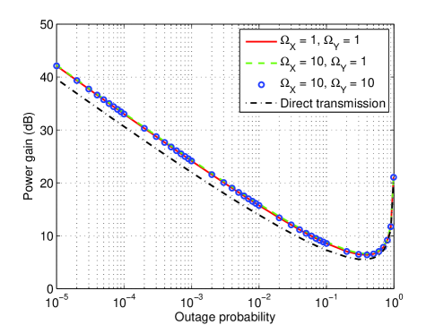
Scenario 2: For a given system OP, we consider the power gain at the relay for OPA $P_{R}^{\ast\ast}\left(x,y,\mu\right)$ as per (22), relative to FPA $P_{R\text{,fixed}}$, such that the power gain is defined as $P_{R\text{,fixed}}/E_{XY}\left[P_{R}^{\ast\ast}\left(x,y,\mu\right)\right]$. Both OPA and FPAย lead to the same OP ($P_{out}^{\text{target}}$) by setting $P_{R\text{,fixed}}=\mu$ such that $\mu$ is determined from (23). We also set $P_{S1}=P_{S2}=\mu$. According to Fig. 3, the power gains are remarkably high when the OP is low, because channel inversion is applied to almost all channel states ($\rho$ has high value). For relatively high OPs (OP between 0.3 and 0.7), the power gain is minimized (but is still above 5 dB), because the nodes are often silent although channel states are not exposed to โ€œdeep fadesโ€. For comparison purposes, the dotted line in Fig. 3 denotes the power gain for truncated channel inversion over a point-to-point communication link in Rayleigh fading, which can be shown to be [13]

$$\frac{1}{-\log\left(1-P_{out}^{\text{target}}\right)\cdot E_{1}\left(-\log\left(1-P_{out}^{\text{target}}\right)\right)}\text{.}$$ (24)

V Conclusion

In this paper, we determined the optimal power allocation at the relay that minimizes the OP of a conventional dual-hop bidirectional AF relaying system with fixed rates, subject to a long-term power constraint at the relay. The end nodes are assumed to be simple communication devices that cannot adapt their output powers. The general solution resembles the truncated channel inversion scheme for point-to-point links. For a special case, we have also derived analytical expressions that allow the evaluation of the cutoff threshold and the OP. The proposed scheme achieves remarkable performance improvements and/or power savings. Most importantly, these benefits come without additional cost for the system, because the required CSI has to be acquired by the relay anyways for adjusting its amplification.

Appendix A Proof of Theorem 1

This proof is inspired by [12]. Theorem 1 is true if the following two propositions are true: Proposition 1: If $P_{R}^{\ast}(x,y)>0$, then PRโˆ—โ€‹(x,y)=PR,sโ€‹tโ€‹(x,y)superscriptsubscript๐‘ƒ๐‘…โˆ—๐‘ฅ๐‘ฆsubscript๐‘ƒ๐‘…๐‘ ๐‘ก๐‘ฅ๐‘ฆP_{R}^{\ast}(x,y)=P_{R,st}(x,y), Proposition 2: $P_{R}^{\ast}(x,y)>0$ if and only if PR,sโ€‹tโ€‹(x,y)โ‰คฯsubscript๐‘ƒ๐‘…๐‘ ๐‘ก๐‘ฅ๐‘ฆ๐œŒP_{R,st}(x,y)\leq\rho.

Proof of Proposition 1: We prove Proposition 1 by contradiction. Assume that Proposition 1 is not true and that $P_{R}^{+}(x,y)$ is the optimal power. Then, $P_{R}^{+}(x,y)$ differs from $P_{R}^{*}(x,y)$ if for some or all $(x,y)$, $P_{R}^{+}(x,y)$ is such that $P_{R}^{+}(x,y)>0$ and PR+โ€‹(x,y)โ‰ PR,sโ€‹tโ€‹(x,y)superscriptsubscript๐‘ƒ๐‘…๐‘ฅ๐‘ฆsubscript๐‘ƒ๐‘…๐‘ ๐‘ก๐‘ฅ๐‘ฆP_{R}^{+}(x,y)\neq P_{R,st}(x,y). Let $\mathcal{S}$ represent the set of $(x,y)$ points for which $P_{R}^{+}(x,y)>0$ and PR+โ€‹(x,y)โ‰ PR,sโ€‹tโ€‹(x,y)superscriptsubscript๐‘ƒ๐‘…๐‘ฅ๐‘ฆsubscript๐‘ƒ๐‘…๐‘ ๐‘ก๐‘ฅ๐‘ฆP_{R}^{+}(x,y)\neq P_{R,st}(x,y). Then, for the points $(x,y)\in\mathcal{S}$, there are three possibilities for the values of $P_{R}^{+}(x,y)$. Either PR+โ€‹(x,y)<PR,sโ€‹tโ€‹(x,y)superscriptsubscript๐‘ƒ๐‘…๐‘ฅ๐‘ฆsubscript๐‘ƒ๐‘…๐‘ ๐‘ก๐‘ฅ๐‘ฆP_{R}^{+}(x,y)<P_{R,st}(x,y) for all $(x,y)\in\mathcal{S}$, or PR+โ€‹(x,y)>PR,sโ€‹tโ€‹(x,y)superscriptsubscript๐‘ƒ๐‘…๐‘ฅ๐‘ฆsubscript๐‘ƒ๐‘…๐‘ ๐‘ก๐‘ฅ๐‘ฆP_{R}^{+}(x,y)>P_{R,st}(x,y) for all $(x,y)\in\mathcal{S}$, or the set $\mathcal{S}$ is comprised of two sets $\mathcal{S}_{1}$ and $\mathcal{S}_{2}$, where for $(x,y)\in\mathcal{S}_{1}$, PR+โ€‹(x,y)<PR,sโ€‹tโ€‹(x,y)superscriptsubscript๐‘ƒ๐‘…๐‘ฅ๐‘ฆsubscript๐‘ƒ๐‘…๐‘ ๐‘ก๐‘ฅ๐‘ฆP_{R}^{+}(x,y)<P_{R,st}(x,y) and for $(x,y)\in\mathcal{S}_{2}$, PR+โ€‹(x,y)>PR,sโ€‹tโ€‹(x,y)superscriptsubscript๐‘ƒ๐‘…๐‘ฅ๐‘ฆsubscript๐‘ƒ๐‘…๐‘ ๐‘ก๐‘ฅ๐‘ฆP_{R}^{+}(x,y)>P_{R,st}(x,y). We will prove that the first two possibilities are not possible and, as a result, the third possibility is also not possible, therefore PR+โ€‹(x,y)=PR,sโ€‹tโ€‹(x,y)=PRโˆ—โ€‹(x,y)superscriptsubscript๐‘ƒ๐‘…๐‘ฅ๐‘ฆsubscript๐‘ƒ๐‘…๐‘ ๐‘ก๐‘ฅ๐‘ฆsuperscriptsubscript๐‘ƒ๐‘…โˆ—๐‘ฅ๐‘ฆP_{R}^{+}(x,y)=P_{R,st}(x,y)=P_{R}^{\ast}(x,y) for all $(x,y)$ for which $P_{R}^{+}(x,y)>0$.

Assume the first possibility, i.e., for $(x,y)\in\mathcal{S}$, PR+โ€‹(x,y)<PR,sโ€‹tโ€‹(x,y)superscriptsubscript๐‘ƒ๐‘…๐‘ฅ๐‘ฆsubscript๐‘ƒ๐‘…๐‘ ๐‘ก๐‘ฅ๐‘ฆP_{R}^{+}(x,y)<P_{R,st}(x,y). Then, $P_{R}^{+}(x,y)$ cannot be the optimal solution since for the considered $(x,y)\in\mathcal{S}$ there is an outage and therefore the outage probability will not change if $P_{R}^{+}(x,y)$ is set to zero. Now assume the second possibility, i.e., for $(x,y)\in\mathcal{S}$, PR+โ€‹(x,y)>PR,sโ€‹tโ€‹(x,y)superscriptsubscript๐‘ƒ๐‘…๐‘ฅ๐‘ฆsubscript๐‘ƒ๐‘…๐‘ ๐‘ก๐‘ฅ๐‘ฆP_{R}^{+}(x,y)>P_{R,st}(x,y). Then, $P_{R}^{+}(x,y)$ again cannot be the optimal power solution since for $(x,y)\in\mathcal{S}$ there is no outage and by setting PR+โ€‹(x,y)=PR,sโ€‹tโ€‹(x,y)superscriptsubscript๐‘ƒ๐‘…๐‘ฅ๐‘ฆsubscript๐‘ƒ๐‘…๐‘ ๐‘ก๐‘ฅ๐‘ฆP_{R}^{+}(x,y)=P_{R,st}(x,y) the outage probability will not change. Finally, the third possibility is a combination of the first two and therefore cannot be true. Hence, Proposition 1 is true.

Proof of Proposition 2: Again, we prove Proposition 2 by contradiction. Let $\mathcal{D}$ represent the set of points for which PR,sโ€‹tโ€‹(x,y)โ‰คฯsubscript๐‘ƒ๐‘…๐‘ ๐‘ก๐‘ฅ๐‘ฆ๐œŒP_{R,st}(x,y)\leq\rho. Then, for the proposed optimal solution, given by (6), the average power is given by

$\displaystyle E_{XY}\{P_{R}^{\ast}(x,y)\}=\int_{x=0}^{\infty}\int_{y=0}^{\infty}P_{R}^{\ast}(x,y)f_{XY}(x,y)dxdy$ (25)
=โˆซโˆซ(x,y)โˆˆ๐’ŸPR,sโ€‹tโ€‹(x,y)โ€‹fXโ€‹Yโ€‹(x,y)โ€‹๐‘‘xโ€‹๐‘‘y=Paโ€‹vโ€‹g.absentsubscript๐‘ฅ๐‘ฆ๐’Ÿsubscript๐‘ƒ๐‘…๐‘ ๐‘ก๐‘ฅ๐‘ฆsubscript๐‘“๐‘‹๐‘Œ๐‘ฅ๐‘ฆdifferential-d๐‘ฅdifferential-d๐‘ฆsubscript๐‘ƒ๐‘Ž๐‘ฃ๐‘”\displaystyle=\int\!\!\!\!\int_{(x,y)\in\mathcal{D}}P_{R,st}(x,y)f_{XY}(x,y)dxdy=P_{avg}. (26)

On the other hand, the outage probability is given by

$$P_{out}^{\ast}=1-\int\!\!\!\!\int_{(x,y)\in\mathcal{D}}f_{XY}(x,y)dxdy,$$ (27)

i.e., there is no outage for those $(x,y)$ for which the relayโ€™s power PRโ€‹(x,y)โ‰ฅPR,sโ€‹tsubscript๐‘ƒ๐‘…๐‘ฅ๐‘ฆsubscript๐‘ƒ๐‘…๐‘ ๐‘กP_{R}(x,y)\geq P_{R,st}, and this is satisfied only for $(x,y)\in\mathcal{D}$, hence comes (27).

Now, let us assume that Proposition 2 is not true and that $P_{R}^{+}(x,y)$ is the optimal power. Since Proposition 1 is true, it follows that if the optimal power $P_{R}^{+}(x,y)$ is nonzero for points $(x,y)$, PR+โ€‹(x,y)=PR,sโ€‹tโ€‹(x,y)superscriptsubscript๐‘ƒ๐‘…๐‘ฅ๐‘ฆsubscript๐‘ƒ๐‘…๐‘ ๐‘ก๐‘ฅ๐‘ฆP_{R}^{+}(x,y)=P_{R,st}(x,y) must hold. However, this is also true for $P_{R}^{*}(x,y)$, i.e., PRโˆ—โ€‹(x,y)=PR,sโ€‹tโ€‹(x,y)superscriptsubscript๐‘ƒ๐‘…๐‘ฅ๐‘ฆsubscript๐‘ƒ๐‘…๐‘ ๐‘ก๐‘ฅ๐‘ฆP_{R}^{*}(x,y)=P_{R,st}(x,y) for $(x,y)\in\mathcal{D}$ and $P_{R}^{*}(x,y)=0$ for $(x,y)\notin\mathcal{D}$. Hence, $P_{R}^{+}(x,y)$ will differ from $P_{R}^{\ast}(x,y)$ if and only if for some or all points $(x,y)\notin\mathcal{D}$, $P_{R}^{+}(x,y)>0$ holds. Moreover, according to Preposition 1, since $P_{R}^{+}(x,y)>0$ then $P_{R}^{+}(x,y)$ must be PR+โ€‹(x,y)=PR,sโ€‹tโ€‹(x,y)superscriptsubscript๐‘ƒ๐‘…๐‘ฅ๐‘ฆsubscript๐‘ƒ๐‘…๐‘ ๐‘ก๐‘ฅ๐‘ฆP_{R}^{+}(x,y)=P_{R,st}(x,y). Hence, $P_{R}^{+}(x,y)$ will differ from $P_{R}^{\ast}(x,y)$ if for some (or all) $(x,y)\notin\mathcal{D}$, PR+โ€‹(x,y)=PR,sโ€‹tโ€‹(x,y)superscriptsubscript๐‘ƒ๐‘…๐‘ฅ๐‘ฆsubscript๐‘ƒ๐‘…๐‘ ๐‘ก๐‘ฅ๐‘ฆP_{R}^{+}(x,y)=P_{R,st}(x,y) holds.

Now, note that PR,sโ€‹tโ€‹(x,y)โ‰คฯsubscript๐‘ƒ๐‘…๐‘ ๐‘ก๐‘ฅ๐‘ฆ๐œŒP_{R,st}(x,y)\leq\rho if and only if $(x,y)\in\mathcal{D}$. As a result, for $(x,y)\notin\mathcal{D}$, PR,sโ€‹tโ€‹(x,y)subscript๐‘ƒ๐‘…๐‘ ๐‘ก๐‘ฅ๐‘ฆP_{R,st}(x,y) must be PR,sโ€‹tโ€‹(x,y)>ฯsubscript๐‘ƒ๐‘…๐‘ ๐‘ก๐‘ฅ๐‘ฆ๐œŒP_{R,st}(x,y)>\rho. Therefore, let us put these points $(x,y)\notin\mathcal{D}$ for which PR+โ€‹(x,y)=PR,sโ€‹tโ€‹(x,y)>ฯsuperscriptsubscript๐‘ƒ๐‘…๐‘ฅ๐‘ฆsubscript๐‘ƒ๐‘…๐‘ ๐‘ก๐‘ฅ๐‘ฆ๐œŒP_{R}^{+}(x,y)=P_{R,st}(x,y)>\rho holds in the set $\mathcal{S}$. Now, since $P_{R}^{+}(x,y)$ has to satisfy the power constraint it follows that the following must hold:

$\displaystyle E_{XY}\{P_{R}^{+}(x,y)\}=\int_{x=0}^{\infty}\int_{y=0}^{\infty}P_{R}^{+}(x,y)f_{XY}(x,y)dxdy$
$\displaystyle=P_{avg}=\int\!\!\!\!\int_{(x,y)\in\mathcal{S}}P_{R}^{+}(x,y)f_{XY}(x,y)dxdy$
$\displaystyle\hskip 22.76219pt+\int\!\!\!\!\int_{(x,y)\in\mathcal{D}}P_{R}^{+}(x,y)f_{XY}(x,y)dxdy.$ (28)

Since for $(x,y)\in\mathcal{S}$, PR+โ€‹(x,y)=PR,sโ€‹tโ€‹(x,y)>ฯsuperscriptsubscript๐‘ƒ๐‘…๐‘ฅ๐‘ฆsubscript๐‘ƒ๐‘…๐‘ ๐‘ก๐‘ฅ๐‘ฆ๐œŒP_{R}^{+}(x,y)=P_{R,st}(x,y)>\rho we can express and denote the first integral in (A) as

โˆซโˆซ(x,y)โˆˆ๐’ฎPR,sโ€‹tโ€‹(x,y)โ€‹fXโ€‹Yโ€‹(x,y)โ€‹๐‘‘xโ€‹๐‘‘y=ฯต,subscript๐‘ฅ๐‘ฆ๐’ฎsubscript๐‘ƒ๐‘…๐‘ ๐‘ก๐‘ฅ๐‘ฆsubscript๐‘“๐‘‹๐‘Œ๐‘ฅ๐‘ฆdifferential-d๐‘ฅdifferential-d๐‘ฆitalic-ฯต\int\!\!\!\!\int_{(x,y)\in\mathcal{S}}P_{R,st}(x,y)f_{XY}(x,y)dxdy=\epsilon, (29)

where $\epsilon>0$ must hold. Otherwise, if $\epsilon=0$ then $\mathcal{S}$ is an empty set in which case $P_{R}^{+}(x,y)=P_{R}^{\ast}(x,y)$. Combining (A) and (29), the second integral in (A) can be written as

$$\int\!\!\!\!\int_{(x,y)\in\mathcal{D}}P_{R}^{+}(x,y)f_{XY}(x,y)dxdy=P_{avg}-\epsilon.$$ (30)

However, since (26) holds, in order for (30) to hold, it follows that for some points $(x,y)\in\mathcal{D}$, $P_{R}^{+}(x,y)$ has to be nonequal to PR,sโ€‹tโ€‹(x,y)subscript๐‘ƒ๐‘…๐‘ ๐‘ก๐‘ฅ๐‘ฆP_{R,st}(x,y). However, according to Preposition 1, for any $(x,y)$, for which PR+โ€‹(x,y)โ‰ PR,sโ€‹tโ€‹(x,y)superscriptsubscript๐‘ƒ๐‘…๐‘ฅ๐‘ฆsubscript๐‘ƒ๐‘…๐‘ ๐‘ก๐‘ฅ๐‘ฆP_{R}^{+}(x,y)\neq P_{R,st}(x,y), $P_{R}^{+}(x,y)=0$ must hold. Hence, in order for (30) to hold, for some points $(x,y)\in\mathcal{D}$, $P_{R}^{+}(x,y)=0$. Let us put the points $(x,y)\in\mathcal{D}$ for which $P_{R}^{+}(x,y)=0$ into the set $\mathcal{D}_{0}$ and the rest of the points in $\mathcal{D}$ for which PR+โ€‹(x,y)=PR,sโ€‹tโ€‹(x,y)superscriptsubscript๐‘ƒ๐‘…๐‘ฅ๐‘ฆsubscript๐‘ƒ๐‘…๐‘ ๐‘ก๐‘ฅ๐‘ฆP_{R}^{+}(x,y)=P_{R,st}(x,y) in the set $\mathcal{D}_{1}$. Therefore, (30) can be written as

$\displaystyle\int\!\!\!\!\int_{(x,y)\in\mathcal{D}}P_{R}^{+}(x,y)f_{XY}(x,y)dxdy=\int\!\!\!\!\int_{(x,y)\in\mathcal{D}_{0}}0\times f_{XY}(x,y)dxdy$
+โˆซโˆซ(x,y)โˆˆ๐’Ÿ1PR,sโ€‹tโ€‹(x,y)โ€‹fXโ€‹Yโ€‹(x,y)โ€‹๐‘‘xโ€‹๐‘‘ysubscript๐‘ฅ๐‘ฆsubscript๐’Ÿ1subscript๐‘ƒ๐‘…๐‘ ๐‘ก๐‘ฅ๐‘ฆsubscript๐‘“๐‘‹๐‘Œ๐‘ฅ๐‘ฆdifferential-d๐‘ฅdifferential-d๐‘ฆ\displaystyle+\int\!\!\!\!\int_{(x,y)\in\mathcal{D}_{1}}P_{R,st}(x,y)f_{XY}(x,y)dxdy
=โˆซโˆซ(x,y)โˆˆ๐’Ÿ1PR,sโ€‹tโ€‹(x,y)โ€‹fXโ€‹Yโ€‹(x,y)โ€‹๐‘‘xโ€‹๐‘‘y=Paโ€‹vโ€‹gโˆ’ฯต.absentsubscript๐‘ฅ๐‘ฆsubscript๐’Ÿ1subscript๐‘ƒ๐‘…๐‘ ๐‘ก๐‘ฅ๐‘ฆsubscript๐‘“๐‘‹๐‘Œ๐‘ฅ๐‘ฆdifferential-d๐‘ฅdifferential-d๐‘ฆsubscript๐‘ƒ๐‘Ž๐‘ฃ๐‘”italic-ฯต\displaystyle=\int\!\!\!\!\int_{(x,y)\in\mathcal{D}_{1}}P_{R,st}(x,y)f_{XY}(x,y)dxdy=P_{avg}-\epsilon. (31)

On the other hand, using $\mathcal{D}=\mathcal{D}_{0}\cup\mathcal{D}_{1}$, (26) can also be written as

โˆซโˆซ(x,y)โˆˆ๐’ŸPR,sโ€‹tโ€‹(x,y)โ€‹fXโ€‹Yโ€‹(x,y)โ€‹๐‘‘xโ€‹๐‘‘ysubscript๐‘ฅ๐‘ฆ๐’Ÿsubscript๐‘ƒ๐‘…๐‘ ๐‘ก๐‘ฅ๐‘ฆsubscript๐‘“๐‘‹๐‘Œ๐‘ฅ๐‘ฆdifferential-d๐‘ฅdifferential-d๐‘ฆ\displaystyle\int\!\!\!\!\int_{(x,y)\in\mathcal{D}}P_{R,st}(x,y)f_{XY}(x,y)dxdy
=โˆซโˆซ(x,y)โˆˆ๐’Ÿ0PR,sโ€‹tโ€‹(x,y)โ€‹fXโ€‹Yโ€‹(x,y)โ€‹๐‘‘xโ€‹๐‘‘yabsentsubscript๐‘ฅ๐‘ฆsubscript๐’Ÿ0subscript๐‘ƒ๐‘…๐‘ ๐‘ก๐‘ฅ๐‘ฆsubscript๐‘“๐‘‹๐‘Œ๐‘ฅ๐‘ฆdifferential-d๐‘ฅdifferential-d๐‘ฆ\displaystyle=\int\!\!\!\!\int_{(x,y)\in\mathcal{D}_{0}}P_{R,st}(x,y)f_{XY}(x,y)dxdy
+โˆซโˆซ(x,y)โˆˆ๐’Ÿ1PR,sโ€‹tโ€‹(x,y)โ€‹fXโ€‹Yโ€‹(x,y)โ€‹๐‘‘xโ€‹๐‘‘y=Paโ€‹vโ€‹g.subscript๐‘ฅ๐‘ฆsubscript๐’Ÿ1subscript๐‘ƒ๐‘…๐‘ ๐‘ก๐‘ฅ๐‘ฆsubscript๐‘“๐‘‹๐‘Œ๐‘ฅ๐‘ฆdifferential-d๐‘ฅdifferential-d๐‘ฆsubscript๐‘ƒ๐‘Ž๐‘ฃ๐‘”\displaystyle+\int\!\!\!\!\int_{(x,y)\in\mathcal{D}_{1}}P_{R,st}(x,y)f_{XY}(x,y)dxdy=P_{avg}. (32)

Subtracting (29) from (A), we obtain

โˆซโˆซ(x,y)โˆˆ๐’Ÿ0PR,sโ€‹tโ€‹(x,y)โ€‹fXโ€‹Yโ€‹(x,y)โ€‹๐‘‘xโ€‹๐‘‘ysubscript๐‘ฅ๐‘ฆsubscript๐’Ÿ0subscript๐‘ƒ๐‘…๐‘ ๐‘ก๐‘ฅ๐‘ฆsubscript๐‘“๐‘‹๐‘Œ๐‘ฅ๐‘ฆdifferential-d๐‘ฅdifferential-d๐‘ฆ\displaystyle\int\!\!\!\!\int_{(x,y)\in\mathcal{D}_{0}}P_{R,st}(x,y)f_{XY}(x,y)dxdy
+โˆซโˆซ(x,y)โˆˆ๐’Ÿ1PR,sโ€‹tโ€‹(x,y)โ€‹fXโ€‹Yโ€‹(x,y)โ€‹๐‘‘xโ€‹๐‘‘ysubscript๐‘ฅ๐‘ฆsubscript๐’Ÿ1subscript๐‘ƒ๐‘…๐‘ ๐‘ก๐‘ฅ๐‘ฆsubscript๐‘“๐‘‹๐‘Œ๐‘ฅ๐‘ฆdifferential-d๐‘ฅdifferential-d๐‘ฆ\displaystyle+\int\!\!\!\!\int_{(x,y)\in\mathcal{D}_{1}}P_{R,st}(x,y)f_{XY}(x,y)dxdy
โˆ’โˆซโˆซ(x,y)โˆˆ๐’ฎPR,sโ€‹tโ€‹(x,y)โ€‹fXโ€‹Yโ€‹(x,y)โ€‹๐‘‘xโ€‹๐‘‘y=Paโ€‹vโ€‹gโˆ’ฯต.subscript๐‘ฅ๐‘ฆ๐’ฎsubscript๐‘ƒ๐‘…๐‘ ๐‘ก๐‘ฅ๐‘ฆsubscript๐‘“๐‘‹๐‘Œ๐‘ฅ๐‘ฆdifferential-d๐‘ฅdifferential-d๐‘ฆsubscript๐‘ƒ๐‘Ž๐‘ฃ๐‘”italic-ฯต\displaystyle-\int\!\!\!\!\int_{(x,y)\in\mathcal{S}}P_{R,st}(x,y)f_{XY}(x,y)dxdy=P_{avg}-\epsilon. (33)

Hence, we obtain the same right hand side in (A) as in (A). Therefore, we can equivalent the left hand sides of (A) and (A), and after some manipulations obtain

โˆซโˆซ(x,y)โˆˆ๐’Ÿ0PR,sโ€‹tโ€‹(x,y)โ€‹fXโ€‹Yโ€‹(x,y)โ€‹๐‘‘xโ€‹๐‘‘ysubscript๐‘ฅ๐‘ฆsubscript๐’Ÿ0subscript๐‘ƒ๐‘…๐‘ ๐‘ก๐‘ฅ๐‘ฆsubscript๐‘“๐‘‹๐‘Œ๐‘ฅ๐‘ฆdifferential-d๐‘ฅdifferential-d๐‘ฆ\displaystyle\int\!\!\!\!\int_{(x,y)\in\mathcal{D}_{0}}P_{R,st}(x,y)f_{XY}(x,y)dxdy
=โˆซโˆซ(x,y)โˆˆ๐’ฎPR,sโ€‹tโ€‹(x,y)โ€‹fXโ€‹Yโ€‹(x,y)โ€‹๐‘‘xโ€‹๐‘‘y.absentsubscript๐‘ฅ๐‘ฆ๐’ฎsubscript๐‘ƒ๐‘…๐‘ ๐‘ก๐‘ฅ๐‘ฆsubscript๐‘“๐‘‹๐‘Œ๐‘ฅ๐‘ฆdifferential-d๐‘ฅdifferential-d๐‘ฆ\displaystyle=\int\!\!\!\!\int_{(x,y)\in\mathcal{S}}P_{R,st}(x,y)f_{XY}(x,y)dxdy. (34)

Since, PR,sโ€‹tโ€‹(x,y)โ‰คฯsubscript๐‘ƒ๐‘…๐‘ ๐‘ก๐‘ฅ๐‘ฆ๐œŒP_{R,st}(x,y)\leq\rho for $(x,y)\in\mathcal{D}_{0}$, and PR,sโ€‹tโ€‹(x,y)>ฯsubscript๐‘ƒ๐‘…๐‘ ๐‘ก๐‘ฅ๐‘ฆ๐œŒP_{R,st}(x,y)>\rho for $(x,y)\in\mathcal{S}$, (A) holds if and only if

$$\int\!\!\!\!\int_{(x,y)\in\mathcal{D}_{0}}f_{XY}(x,y)dxdy\geq\int\!\!\!\!\int_{(x,y)\in\mathcal{S}}f_{XY}(x,y)dxdy$$ (35)

holds, where equality holds if and only if $\epsilon=0$, in which case both $\mathcal{D}_{0}$ and $\mathcal{S}$ are empty sets, which means that $P_{R}^{+}(x,y)=P_{R}^{\ast}(x,y)$.

On the other hand, the outage probability obtained with $P_{R}^{+}(x,y)$ is given by

$$P_{out}^{+}=1-\int\!\!\!\!\int_{(x,y)\in\mathcal{D}_{1}}f_{XY}(x,y)dxdy-\int\!\!\!\!\int_{(x,y)\in\mathcal{S}}f_{XY}(x,y)dxdy,$$ (36)

i.e., there is no outage for those $(x,y)$ for which the relayโ€™s power PRโ€‹(x,y)โ‰ฅPR,sโ€‹tsubscript๐‘ƒ๐‘…๐‘ฅ๐‘ฆsubscript๐‘ƒ๐‘…๐‘ ๐‘กP_{R}(x,y)\geq P_{R,st}, and for $P_{R}^{+}(x,y)$ this holds only for $(x,y)\in\mathcal{D}_{1}$ and $(x,y)\in\mathcal{S}$, which leads to (36). Inserting the bound in (35) into (36), we obtain

$\displaystyle P_{out}^{+}\geq 1-\int\!\!\!\!\int_{(x,y)\in\mathcal{D}_{1}}f_{XY}(x,y)dxdy-\int\!\!\!\!\int_{(x,y)\in\mathcal{D}}f_{XY}(x,y)dxdy$
$\displaystyle=1-\int\!\!\!\!\int_{(x,y)\in\mathcal{D}}f_{XY}(x,y)dxdy=P_{out}^{\ast}\,,$ (37)

where equality holds if and only if $\mathcal{S}$ in a empty set in which case $P_{R}^{+}(x,y)=P_{R}^{\ast}(x,y)$. Hence, $P_{out}^{+}>P_{out}^{*}$ for any PR+โ€‹(x,y)โ‰ PRโˆ—โ€‹(x,y)superscriptsubscript๐‘ƒ๐‘…๐‘ฅ๐‘ฆsuperscriptsubscript๐‘ƒ๐‘…๐‘ฅ๐‘ฆP_{R}^{+}(x,y)\neq P_{R}^{*}(x,y). This concludes the proof.

Appendix B Proof of Theorem 3

The solution to (21) must satisfy Preposition 1 in Appendix A. One solution which satisfies Preposition 1 is $P_{R}^{\ast}(x,y)$ given by (22). Let us denote any solution other than $P_{R}^{\ast}(x,y)$ that still satisfies Preposition 1 as $P_{R}^{+}(x,y)$. Then, following a similar procedure as in the proof of Preposition 2 in Appendix A, we can obtain the expressions for the system OP and average relay powers resulting from $P_{R}^{\ast}(x,y)$ and $P_{R}^{+}(x,y)$. Preposition 2 of Appendix A proves that, if the average values of $P_{R}^{\ast}(x,y)$ and $P_{R}^{+}(x,y)$ are equal, then the system OP resulting from solution $P_{R}^{\ast}(x,y)$ is less than the system OP resulting from solution $P_{R}^{+}(x,y)$. Following a similar approach, if we set the system OPs resulting from the solutions $P_{R}^{\ast}(x,y)$ and $P_{R}^{+}(x,y)$ to be equal, then the average value of $P_{R}^{\ast}(x,y)$ is always less than the average value of $P_{R}^{+}(x,y)$. Hence, $P_{R}^{\ast}(x,y)$ gives the minimal average relay output power for a given system OP. This completes the sketch of the proof.

References

  • [1] B. Rankov and A. Wittneben, โ€Spectral Efficient Protocols for Half-Duplex Fading Relay Channelsโ€, IEEE J. Sel. Areas Commun., vol. 25, no. 2, pp. 379โ€“389, Feb. 2007
  • [2] S. Zhang, S. C. Liew, and P.P. Lam, โ€Physical-layer Network Codingโ€, Proc. ACM MobiCom, 2006, pp. 358-365
  • [3] S. Katti, S. Gollakota, and D. Katabi, โ€Embracing Wireless Interference: Analog Network Codingโ€, Proc. ACM SIGCOMM, 2007, pp. 397-408
  • [4] Q. Li, S. H. Ting, A. Pandharipande, and Y. Han, โ€Adaptive Two-Way Relaying and Outage Analysisโ€, IEEE Trans. Wireless Commun., vol. 8, No. 6, pp. 432-439, June 2009
  • [5] R. H. Y. Louie, Y. Li, and B. Vucetic, โ€Practical Physical Layer Network Coding for Two-Way Relay Channels: Performance Analysis and Comparison, IEEE Trans. Wireless Commun., vol. 9, no. 2, pp. 764โ€“777, Feb. 2010
  • [6] Z. Yi, M. C. Ju, and Il-Min Kim, โ€Outage Probability and Optimum Power Allocation for Analog Network Codingโ€, IEEE Trans. Wireless Commun., vol. 10, No. 2, pp. 407-412, Feb. 2011
  • [7] X. J. Zhang, and Y. Gong, โ€Adaptive power allocation in two-way amplify-and-forward relay networksโ€, Proc. ICC 2009, pp. 1-5
  • [8] Y. Zhang, Y. Ma, and R. Tafazolli, โ€Power Allocation for Bidirectional AF Relaying over Rayleigh Fading Channelsโ€, IEEE Commun. Letters, vol. 14, no. 2, pp. 145-147, Feb. 2010
  • [9] Y Li, X. Zhang, M. Peng, and W. Wang, โ€Power Provisioning and Relay Positioning for Two-Way Relay Channel With Analog Network Codingโ€, IEEE Sig. Proc. Letters, vol. 18, no. 9, pp. 517-520, Sept. 2011
  • [10] N. Ahmed, M. A. Khojastepour, A. Sabharwal, and B. Aazhang, โ€Outage minimization with limited feedback for the fading relay channelโ€, IEEE Trans. on Commun., vol. 54, no. 4, Apr. 2006
  • [11] D. Gunduz, and E. Erkip, โ€Opportunistic cooperation by dynamic resource allocationโ€, IEEE Trans. Wireless Commun., vol. 6, no. 4, pp. 1446-1454, Apr. 2007
  • [12] G. Caire, G. Taricco, and E. Biglieri, โ€Optimum power control over fading channelsโ€, IEEE Trans. Info. Theory, vol. 45, no. 5, pp. 1468-1489, July 1999
  • [13] A. J. Goldsmith and P. Varaiya, โ€œCapacity of fading channels with channel side informationโ€, IEEE Trans. Info. Theory, vol. 43, no. 6, pp. 1986-1992, Nov. 1997
  • [14] M. Abramowitz and I.A. Stegun, Handbook of Mathematical Functions with Formulas, Graphs, and Mathematical Tables, 9th Ed. Dover, 1970