The derivative discontinuity of the exchange-correlation functional

Abstract

The derivative discontinuity is a key concept in electronic structure theory in general and density functional theory in particular. The electronic energy of a quantum system exhibits derivative discontinuities with respect to different degrees of freedom that are a consequence of the integer nature of electrons. The classical understanding refers to the derivative discontinuity of the total energy as a function of the total number of electrons ($N$), but it can also manifest at constant $N$. Examples are shown in models including several Hydrogen systems with varying numbers of electrons or nuclear charge ($Z$), as well as the 1-dimensional Hubbard model (1DHM). Two sides of the problem are investigated: first, the failure of currently used approximate exchange-correlation functionals in DFT and, second, the importance of the derivative discontinuity in the exact electronic structure of molecules, as revealed by full configuration interaction (FCI). Currently, all approximate functionals miss the derivative discontinuity, leading to basic errors that can be seen in many ways: from the complete failure to give the total energy of H₂ and H${}_{2}^{+}$, to the missing gap in Mott insulators such as stretched H₂ and the thermodynamic limit of the 1DHM, or a qualitatively incorrect density in the HZ molecule with two electrons and incorrect electron transfer processes. Description of the exact particle behavior of electrons is emphasized, which is key to many important physical processes in real systems, especially those involving electron transfer, and offers a challenge for the development of new exchange-correlation functionals.

I introduction

The total energy in density functional theory (DFT) is given by

$$E[\rho]=T_{s}[\rho]+\int\!\!\rho(\mathbf{r})v_{\mathrm{ext}}(\mathbf{r})\mathrm{d}\mathbf{r}+J[\rho]+E_{xc}[\rho]$$ (1)

with explicit expressions for the non-interacting kinetic energy,

$$T_{s}[\rho]=\sum_{i}\langle\phi_{i}|-\frac{1}{2}\nabla^{2}|\phi_{i}\rangle,$$ (2)

and Coulomb energy

$$J[\rho]=\frac{1}{2}\iint\!\!\frac{\rho(\mathbf{r})\rho(\mathbf{r}^{\prime})}{|\mathbf{r}-\mathbf{r}^{\prime}|}\mathrm{d}\mathbf{r}\mathrm{d}\mathbf{r}^{\prime}.$$ (3)

All the unknown complexity and many-body physics are in the remaining term, the exchange-correlation functional, $E_{xc}[\rho]$. The orbitals used to construct the density are solutions of the Kohn-Sham equation

$$\left(-\frac{1}{2}\nabla^{2}+v_{\mathrm{ext}}(\mathbf{r})+\int\!\!\frac{\rho(\mathbf{r}^{\prime})}{|\mathbf{r}-\mathbf{r}^{\prime}|}\mathrm{d}\mathbf{r}^{\prime}+v_{xc}(\mathbf{r})\right)\phi_{i}(\mathbf{r})=\epsilon_{i}\phi_{i}(\mathbf{r})$$ (4)

where the exchange-correlation potential is given by the functional derivative of the exchange-correlation energy, $v_{xc}(\mathbf{r})=\frac{\delta E_{xc}[\rho]}{\delta\rho(\mathbf{r})}$. This is exact DFT. With the exact functional, the solution of the Kohn-Sham equation (Eq. 4) to minimise the total energy (Eq. 1) yields the exact solution of the Schrödinger equation. However, the exact form of $E_{xc}[\rho]$ is unknown and it is necessary to use density functional approximations (DFA). DFAs have both an approximate energy expression, $E_{xc}^{{\rm DFA}}$, and approximate Kohn-Sham potential, $v_{xc}^{\mathrm{DFA}}(\mathbf{r})$, giving rise to approximate density, $\rho^{\mathrm{DFA}}(\mathbf{r})$, and eigenvalues, $\{\epsilon_{i}^{\mathrm{DFA}}\}$.

I.1 Density functional approximations

There are many different functional forms, starting with semilocal functionals that range from the local density approximation (LDA) Dirac (1930); Vosko et al. (1980); Perdew and Wang (1992) to the generalized gradient approximation (GGA) Becke (1988a); Lee et al. (1988); Perdew et al. (1996); Perdew (1986); Handy and Cohen (2001) and meta-GGA functionals Becke (1988b); Becke and Roussel (1989); Tao et al. (2003); Zhao and Truhlar (2006). There are also many functionals that mix in Hartree-Fock exact exchange in some manner, such as hybrid functionals with a varying degree of constant admixture of exact exchange, from B3LYP (20% HF) to PBE0 (25%) to M06-2X (58%) and M06-HF (100%) Becke (1993a, b); Stephens et al. (1994); Adamo and Barone (1999); Becke (1997); Hamprecht et al. (1998); Keal and Tozer (2005). In the last decade many functionals have emerged that examine the idea of range-separation pioneered by Andreas Savin, with functionals that include all the long-range part of HF exchange (LC-BLYP, LC-$\omega$PBE) to CAMB3LYP and $\omega$B97xd Iikura et al. (2001); Yanai et al. (2004); Vydrov and Scuseria (2006); Chai and Head-Gordon (2008) to mixing in only the short range part of Hartree-Fock Heyd et al. (2003, 2006). All these functionals use only the occupied orbitals and fit in a general sense to the first four rungs of Jacob’s Ladder of density functional approximations Perdew and Schmidt (2001). On the fifth rung there have been some ideas that use the unoccupied orbitals and eigenvalues in functionals such as B2PLYP Grimme (2006), which mix in some MP2-like terms or the random phase approximation (RPA), for example direct RPA (dRPA) Bohm and Pines (1952); Furche (2008) which uses the Coulomb only response in the adiabatic fluctuation dissipation theorem.

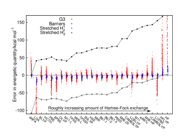
Figure 1: Calculated errors in thermochemical heats of formation (red dots), reaction barrier heights (blue dots), and also the errors of stretched H${}_{2}^{+}$ (black circle) and stretched H₂ (black dots) for a wide variety of functionals.

Fig. 1 presents a similar figure to Fig. 8 of Ref. Cohen et al. (2012) to illustrate the performance of a large range of functionals for a set of thermochemical data (the heats of formation of the G3 set Curtiss et al. (2000)) and a set of reaction barrier heights Zhao et al. (2004, 2005). For each of the functionals the calculated error of an energetic quantity for every individual molecules is represented by a single dot, in Fig. 1 each red dot is the error in the heat of formation of a molecule in the G3 set and each blue dot is one of the errors in a reaction barrier height. The results for dRPA for thermochemistry are only for the G2 set Curtiss et al. (1997) and and the barriers are the DHB24 set Zheng et al. (2009) and the results for these are taken from the paper and supplementary information of Ref. Yang et al. (2013a) all other calculations are post-B3LYPCohen et al. (2012). This allows one to see the performance of many different functionals in a global manner. In addition to the usual thermochemistry and barriers for each individual functional we also plot the errors for the two simplest molecules in the whole of chemistry infinitely stretched H${}_{2}^{+}$ and infinitely stretched H₂. Individually these molecules are known to be difficult for functionals to describe with stretched H${}_{2}^{+}$ Merkle et al. (1992) epitomising self-interaction error Perdew and Zunger (1981); Mori-Sánchez et al. (2008) and stretched H₂ the problem of static correlationCohen et al. (2008). The errors for these two molecules, as one can see in Fig. 1, are very large but importantly connected. One can see that in changing functionals it is only possible to improve one error but with a corresponding failure on the other, the two seem connected. No functional is able to describe correctly these two simple molecules. It is this connection between different systems that epitomises the challenge of making one functional that can act discontinuously for different particle numbers, which is a markedly different challenge to the usual atomization energies of the G3 set or barrier heights.

While there has been much improvement in the prediction of thermochemistry and reaction barriers over many years, using many different ideas in functionals, there is no functional that can reproduce the energy of these two simple systems.This can be viewed in two ways: one, is that the challenges of chemistry are not so related to the electronic structure of stretched H₂/H${}_{2}^{+},$ which has lead to the concept that DFT works well as long as one does not stretch bonds. It is hoped hope that these errors do not cause a problem in the systems under study. However, the other view is that if current approximations are not able to correctly describe these two simple systems, then it should not be expected that for an unknown chemical they will give the correct answer. The key is not to just focus on the system, but on the behavior of the electrons themselves. The errors in stretched H₂/H${}_{2}^{+}$ show a fundamental failure to correctly describe the electrons in those molecules and, as such, the description of similar electronic structure in many other systems will also fail. If these errors are not corrected, the inconsistencies of functionals will continue to dominate over the true behavior of electrons.

I.2 Newer ideas in functionals

There are several groups working on new ideas in DFT, which is greatly needed to address the qualitative problems that can be seen in simple model systems. For example, Gori-Giorgi and coworkers are looking at the strictly-interacting $\lambda\rightarrow\infty$ limit of the adiabatic connection for ideas based on strictly correlated electrons (SCE) Gori-Giorgi et al. (2009); Gori-Giorgi and Seidl (2010); Mirtschink et al. (2013). The concept of SCE can deal with problem of stretched H₂. Other notions beyond DFT, such as partition DFT, have been developed to attempt to tackle some of these problems Nafziger and Wasserman (2013). Burke and coworkers have also looked at exact Kohn-Sham calculations in 1D using the exact functional by doing a DMRG calculation via a density perspective Wagner et al. (2012). The particle-particle RPA (ppRPA) has been developed for electronic structure theory by van Aggelen, Yang and Yang van Aggelen et al. (2013), showing a relation with ladder coupled-cluster Peng et al. (2013); Scuseria et al. (2013). Becke also has used real space ideas to address non-dynamical correlation and delocalization error using inverse hole models Becke (2005, 2013). There are schemes to combat this issue beyond DFT, from CASDFT Savin (1988); Grafenstein and Cremer (2000) to embedding methods in quantum chemistry Knizia and Chan (2012, 2013); Huang et al. (2011); Libisch et al. (2012) as well as ideas in density-matrix functional theory. Hopefully, the culmination of these theories will provide new functionals to be able to apply to a large spectrum of chemistry and physics without the drawbacks of many of the currently used functionals.

I.3 Challenge for DFAs

In this paper we highlight the difficult question of the derivative discontinuity of the exchange-correlation functional. The issue of describing the energies of stretched H${}_{2}^{+}$ and stretched H₂ with the same functional epitomises this challenge in a clear manner, but there are many other ways to the view the problem. This is a much larger issue than just that of stretching molecules, it is to correctly describe the energy of the electrons in all situations. An improved functional should be able to accurately describe the general behaviour of electrons, especially in interesting physical processes where competing effects act equally. This is the key problem to tackle, so that DFT calculations can describe the important chemical reactions and responses to electric and magnetic fields that are needed for the correct understanding of the behaviour of electrons in enzyme catalysis, Li-ion batteries, solar cells and many other technological applications.

II Derivative Discontinuity of the energy versus number of electrons

The famous paper from Perdew, Parr, Levy and Balduz Jr in 1982 Perdew et al. (1982) showed that the energy for a system with fractional electron number is given by a straight line connecting integer electron numbers

$$E(N+\delta) = (1-\delta)E(N)+\delta E(N+1)$$ (5)

$$\rho_{N+\delta}(\mathbf{r}) = (1-\delta)\rho_{N}(\mathbf{r})+\delta\rho_{N+1}(\mathbf{r}).$$ (6)

The energy and density are piecewise linear with straight lines connecting the integer points. This means that, at the integers, both the energy and density show (or can show) derivative discontinuities. In most situations there is a large discontinuity in the density on changing electron number. This is especially true in closed shell molecules where the density difference between last electron added (given by $\rho_{N}-\rho_{N-1})$ is very spatially different from where the next electron is added $(\rho_{N+1}-\rho_{N}).$ Or, in other words, when the frontier orbitals are spatially (and energetically) different.

We will focus on understanding manifestations of the derivative discontinuity in the total energy of integer systems. However, much of the understanding of the DD is often related to the exact Kohn-Sham potential, which was shown by Levy and Perdew Perdew and Levy (1983) to undergo a jump by a constant when passing through the integer. This constant, $C,$ is the derivative discontinuity.

$$v_{xc}^{N-\epsilon}(\mathbf{r}) = v_{xc}^{N}(\mathbf{r})$$

$$v_{xc}^{N+\epsilon}(\mathbf{r}) = v_{xc}^{N}(\mathbf{r})+C.$$

This can be confusing to understand. For example, for a functional such as LDA, what does it matter if the potential is shifted by a constant? If that shifted potential is put in to the Kohn-Sham equations Eq. 4, it will give rise to identical orbitals and density, however the eigenvalues are shifted by a constant. If those orbitals and density are put in to the energy expression Eq. 1 an identical energy will be obtained. This means that there is a discontinuous change only in our eigenvalues, not in the total energy. This question is part of the challenge of understanding the importance of exact conditions in DFT, in this case the relation between the derivative discontinuity and the energy expression in relation to the potential. We think that the shift in the potential comes from something in the total energy expression that is missing in LDA. It is this missing part of the LDA energy expression that is the key question to be searching for. This whole discussion is fraught with problems, but we want to cement our understanding by finding molecules (or model systems) where the question becomes clarified. In this work we will elaborate on the implications of the derivative discontinuity for the energies of systems with integer number of electrons, where there is no need to invoke eigenvalues, fractional numbers of electrons or ensemble densities.

II.1 Hydrogen atom and flat plane condition

Consider the energy of a hydrogen atom, going from H⁺ to H^-, but with a possibly fractional number of electrons, $N=n_{\alpha}+n_{\beta}$, $0\leq n\leq 2$ and also $n_{\alpha}\leq 1$ and $n_{\beta}\leq 1$. This is a very simple system to help understand fractional numbers of electrons. The behavior of the exact energy is given by the the flat plane condition, which is a very stringent test of approximate functionals Mori-Sánchez et al. (2009). Especially important is the understanding of the behaviour at $N=1,$ where two planes intersect giving an energy derivative discontinuity, and to consider adding and subtracting fractional numbers of electrons. More complicated surfaces were also investigated in the work of Gal and Geerlings Gal and Geerlings (2010).

DFAs really struggle to describe the flat plane and they completely fail to recover the discontinuous behaviour seen in the exact behaviour of the energy at $N=1$. It is this failure that is connected to (or the root of) all the subsequent failures that we see. For the $n_{\alpha}=n_{\beta}$ line, approximate functionals massively fail, as they need to know that on going from $E[0.4\alpha,0.4\beta]\rightarrow E[0.5\alpha,0.5\beta]\rightarrow E[0.6\alpha,0.6\beta]$ they have passed through one electron. Compare this with the edge of the flat plane, $E[0.8\alpha,0\beta]\rightarrow E[\text{1.0$\alpha$,0$\beta$]$\rightarrow$E[1.0$\alpha$,0.2$\beta$]}$, where there is a change of the orbital being occupied (from $\alpha$ to $\beta$) on passing through the integer. It is clear from the energy expressions of Eq. 1 that without a change of orbitals, the only term that can give the discontinuity is the exchange-correlation term. This is where the failure of current functionals and the challenge for future functionals lie. There is also a large discontinuity in the density with electron addition $f_{+}=\rho_{H^{-}}-\rho_{H}$ very spatially different from electron removal $f_{-}=\rho_{H}-\rho_{H^{+}}$.

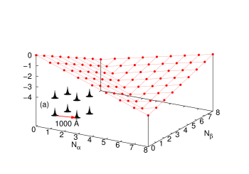
Figure 2: The total energy for different number of electrons of an H₈ cube separated by 1000 Å (sketched in inset (a)), with one basis function per Hydrogen, calculated by FCI with up to $8\alpha$ and $8\beta$ electrons.

II.1.1 Hydrogen atom with 1 basis function

To simplify the argument, it is useful to consider the calculation of the Hydrogen atom just using a single basis function. The main reason to do this is that now the density is constrained by the basis function to be completely determined up to a factor such that it is no longer discontinuous on passing through $N=1$, with $\rho_{H^{-}}=2\rho_{H}$. A secondary point is that the discontinuity in the energy is in this case greatly enhanced if the basis function is chosen as $\eta({\bf r})=\frac{1}{\sqrt{\pi}}e^{-r}$ (note the discontinuity could be reduced slightly if the basis function is chosen to be give the correct density at $N=2$, i.e. $\eta({\bf r})\propto\sqrt{\rho_{{\rm H}^{-}}({\bf r})}$). Additionally, the use of one basis function provides a direct connection to the Hubbard model where there is also one basis function per site. One of the features of the flat plane condition is that it considers fractional numbers of electrons, which can lead to conceptual confusion as well as technical challenges in extending methods to fractional numbers of electronsYang et al. (2013b); Steinmann and Yang (2013). However, the flat plane condition was developed to explain the root cause in functionals of a general problem that affects real systems and hence can be equally seen in integer systems.

Let us consider a cube of 8 Hydrogen atoms (each with one basis function). For this system FCI calculations can be easily carried out with different numbers of electrons and spins as in Fig. 2, where we have used a very large (1000 Å) distance along the edge of the cube just for simplicity. The density at each H atom is constrained by the basis set so an increase in energy happens when more than one electron per site is added; this is exactly the same as in the Hubbard model, where the on-site repulsion $U$ causes an increase in energy past half-filling. Of course if the basis set allowed, these electrons would be unbound from the molecule (or as in a real H atom they would be much more diffuse to slightly lower in energy). These issues could be circumvented by changing the nucleus to be a He atom so that the attraction to the nucleus makes it much more favourable in energy. The real challenge for functionals it is to give the line of discontinuity crossing 8 electrons (one electron per H atom).

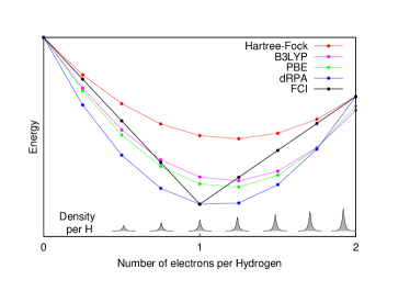
Figure 3: Energy of closed shell H₈ with a minimal basis set with 0, 2, 4, 6, 8, 10, 12, 14 and 16 electrons. Methods such as RHF, dRPA, BLYP and B3LYP completely miss any discontinuous behaviour in the total energy.

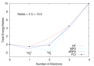
(a) Energy of the two site Hubbard model with different numbers of electrons calculated with FCI, HF, MP2 and dRPA. $N=1$ is like a stretched H${}_{2}^{+}$ molecule and $N=2$ is like a stretched H₂ and we can see how the errors of methods such as HF, dRPA and MP2 lead to an incorrect gap at $N=2$.

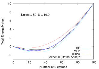
(b) Energy of a 50 site 1-d periodic Hubbard model with between 0 and 100 electrons calculated with HF, MP2 and dRPA compared with the exact Bethe-Ansatz result. In contrast to the exact Bethe-Ansatz result the DFA methods completely fail to give any sort of discontinuous behaviour at half-filling (50 electrons).

Figure 4:

Let us just consider a single line in the flat plane with $N_{\alpha}=N_{\beta}$, i.e. only closed shell systems. For this line calculations with any functional can be easily carried out as the density and orbitals are known. Fig. 3 shows the performance of HF, dRPA, PBE, B3LYP and FCI. First, the FCI energy with 16 electrons (i.e. two electrons per site) is the same as HF, as the basis set does not allow for any electron correlation. As DFT functionals such as PBE and B3LYP treat correlation in a completely different manner, they have a slightly lower energy at 16 electrons. We could have considered just exchange functionals but have left in the correlation part so that one can see the relatively small effect of dynamic correlation functionals.

Overall, all the approximate methods completely fail to reproduce any discontinuous behaviour of the total energy, and have a smooth behaviour in contrast to the correct answer of FCI. For less that one electron per site the energy decreases by $-0.5$ per electron, and for more than one electron per site the energy increases by $0.13$ per electron. This H₈ molecule clearly illustrates the same physics as fractional electron numbers in one single H atom and also the same error of functionals, the missing derivative discontinuity. This example illustrates the important point that the missing derivative discontinuity in functionals can manifest itself as an error in the energy of integer systems.

II.2 The 1-dimensional Hubbard model

The Hubbard model Hubbard (1963)

$$\hat{H}=-t\sum_{i}(c_{i}^{\dagger}c_{i+1}+h.c.)+U\sum_{i}n_{i\alpha}n_{i\beta}$$

is a much studied system in strongly correlated condensed matter physics as it is a very simple model which describes interacting electrons in narrow energy bands, and which has been applied to problems as diverse as superconductivity, band magnetism, and the metal-insulator transition. The interplay between the delocalized hopping, $t$, and the localised repulsion, $U$, can lead to interesting balance in physical behaviors. Here we will examine the 1-dimensional Hubbard model (1D-HM) to highlight the connection with Hydrogen atoms and derivative discontinuities, especially that seen at half filling. For the 1D-HM the exact answer is known in the thermodynamic limit using the Bethe-Ansatz, for example, the gap of the 1D-HM is given by Lieb and Wu (1968)

$$E_{{\rm gap}}^{{\rm BA}}=U-4+8\int_{0}^{\infty}\frac{J_{1}(x)}{x[1+\exp(Ux/2)]}\mathrm{d}x$$

where $J_{1}$ is the first order Bessel function.

The Hubbard model is symmetric around half filling (except that above half-filling an electron-interaction term is included) i.e. for a system with 2$N$ sites and doping fraction of $M/N$

$$E[N-M]=E[N+M]+MU.$$ (7)

This leads to a clear picture of the derivative discontinuity that exists in the Hubbard model at half-filling, and raises the question of how to include this physics in a functional. This is exactly the same as the question of how to get a gap at the whole line in the flat plane condition of the Hydrogen atom. The key of how to generally put this in a functional is distinct from how to predict the gap of the Hubbard model, where of course the knowledge of the system and the property in Eq. (7) can be more specifically used to get the gap. For example, Capelle and coworkers Lima et al. (2003); França et al. (2012); Capelle and Campo (2013) have several specific functionals (BA-LDA (LSOC, FVC)) and different parameterizations that are able to give the gap of the Hubbard model.

We consider finite Hubbard rings (chains with periodic boundary conditions) where exact results can be computed using FCI. The size of the chain can be increased and the large number of site limit corresponds to the thermodynamic limit. The two site Hubbard model has a very clear connection to infinitely stretched Hydrogen molecule, with one electron this corresponds to H${}_{2}^{+}$ and with two electrons to H₂. Fig. 4 shows the total energy for two different Hubbard models, both with $t=1$ and a large values of $U=10$. The two site model is examined in Fig 4a. The performance of methods is exactly as expected from calculations on stretched H${}_{2}^{+}$/H${}_{2};$ HF and MP2 are good for one electron but fail for two electrons (HF is too high due to static correlation error and MP2 diverges to $-\infty$ as $U$ is increased). dRPA performs better for two electrons at the cost of a massive error for one electron Mori-Sánchez et al. (2012). Here, dRPA would still give a gap at half-filling ($N=2$). However, as shown for the 50 site model in Fig. 4b, the real problem arises in approaching the thermodynamic limit, where methods such as HF, dRPA or even MP2, smooth out and all semblance of a gap at half-filling disappears. However, the exact Bethe-Ansatz results give a very large gap. The complete failure of functionals to give a derivative discontinuity means that their results on the Hubbard model are completely physically incorrect as they miss one of the key behaviours of true Hubbard electrons.

II.3 Fractional nuclei: HZ^{2e}

A picture of the discontinuous behaviour of the electrons is beautifully illustrated in the two electron example of an H₂ like molecule changing the nuclear charge of one of the protons to be fractional, giving HZ^{2e} Cohen and Mori-Sánchez (2014). This encompasses a set of systems connected by a very simple change to the one-electron potential. This is a smooth and continuous change to the Hamiltonian, however, how does the electronic structure behave on these small changes, does it also change smoothly? As demonstrated in Fig. 5 the answer is, of course, that it depends. In some cases, as illustrated in short bond distances of HZ^{2e}, the electron also moves smoothly on this change. However, at long distances, the electron moves discontinuously, being either on the H or the Z, it is not shared between them.

The true behaviour of electrons, as given by FCI calculations, is simple to understand for HZ^{2e} at stretched bond lengths. When $Z=0$ there are two electrons on the H atom (i.e. H${}^{-})$ and as $Z$ increases an electron moves from the H to the Z when the energy of putting one electron on the Z atom gives a lower energy. This occurs when the energy of one electron on the $Z$ atom, $E=-\frac{Z^{2}}{2}$, is lower than the negative of the electron affinity of the H atom (EA(H)=$-0.0277a.u.$). This happens at $Z=0.235$. The atoms are too far apart to be bonded and no fractional electron transfer happens, as can be understood from the PPLB straight line interpolation of the true FCI energy of Eq. (5). Something similar happens around $Z=1.67$, where it becomes more energetically favourable to have two electrons on the Z atom and none on the H (at that point the electron affinity of the Z atom crosses $0.5$). This is simple and clear, it is just the qualitative failure of functionals that is surprising.

Consider $Z=1,$ i.e. the H₂ molecule, all functionals get a qualitatively correct density due to the symmetry of the problem. However, they respond completely incorrectly to a small change in one of the atoms. DFAs smoothly move electrons when in fact they should not do so; no fractional charge is seen from FCI calculations. This turns the well known static-correlation error in the energy into a qualitative failure in the density. Approximate energy functionals are not able to describe the integer nature of electrons and they do not penalise correctly the splitting up of an electron in these stretched cases.

The HZ^{2e} system is very interesting and has advantages over very similar physics that can be seen in asymmetric Hubbard models or Anderson models in that functionals can be simply tested and their performance directly analyzed in real space. The conclusion is that they all fail for this problem. The reasons can be traced back to the failure of functionals for the closed-shell line of the flat plane (see Fig. 3). Along that line these functionals have no clear knowledge that they have passed through one electron and this translates into the problems seen in the density for these systems. This example is very illustrative but it is a slightly hard test as it requires self-consistent determination of the density. For methods such as dRPA, which is usually evaluated with PBE (sometimes HF) orbitals, it requires a self-consistent calculation Mori-Sánchez et al. (2014) to highlight a problem in the density rather than energy, as carried out for Fig. 5 .

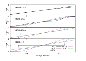
Figure 5: Occupation of Z atom, $\langle n_{Z}\rangle$, as the nuclear charge on the Z atom is varied at four different bond lengths comparing FCI and several different approximate DFT functionals.

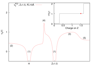
Figure 6: Kohn-Sham potential of HZ^{2e} for $Z=1.5$ with a bond length of 10 Å. The features of the potential given by labels (1)-(5) are explained in the text and the inset shows the number of electrons on the Z atom for all HZ^{2e} systems.

III The derivative discontinuity as a challenge for $v_{xc}(\mathbf{r})$?

Our main view is that the derivative discontinuity must be understood as a challenge for the energy, $E_{xc}[\rho]$. For example, in the HZ^{2e} problem, a functional that correctly gives the energy for the transfer of an electron would also give a qualitatively correct electron density and energy. For the set of HZ^{2e} systems, if the energy is wrong then the density will follow, giving rise to a qualitatively incorrect transfer. An equivalent, but in our view, confusing way to phrase this challenge is about the Kohn-Sham potential. To illustrate this point take the case $Z=1.5$ for a stretched geometry as an example. Let us ask the question what is the exact Kohn-Sham potential that gives rise to integer number of electrons on each atom. This is clear in the HZ^{2e} system, as we have access to the exact Kohn-Sham potential, $v_{s}(\mathbf{r})$ and $v_{xc}(\mathbf{r})$. This comes from a very simple rearrangement of Eq. 4, substituting in the fact that the density is only made of one orbital, $\phi_{1}(\mathbf{r})=\sqrt{\rho(\mathbf{r})/2}$, giving rise to

$$v_{s}(\mathbf{r})+\epsilon_{1} = \frac{\nabla^{2}\rho}{4\rho}-\frac{(\nabla\rho)^{2}}{8\rho^{2}}$$ (8)

$$v_{xc}(\mathbf{r})+\epsilon_{1} = \frac{\nabla^{2}\rho}{4\rho}-\frac{(\nabla\rho)^{2}}{8\rho^{2}}-v_{\mathrm{ext}}(\mathbf{r})-v_{J}(\mathbf{r}).$$ (9)

In this case, the exact Kohn-Sham potential is directly available from an exact density in a FCI calculation.

Many plots have been seen in the literature, in both ground state and time-dependent analysis of the potential, for example Perdew (1985); Gritsenko et al. (1995); Helbig et al. (2009); Tempel et al. (2009); Hellgren and Gross (2012). The way to understand any features of the potential is that they are present as a consequence given a particular electron density, i.e. the exact Kohn-Sham potential (Eq. 8) is just a restatement of the density. This is shown in Fig. 6, where we just evaluate Eq. 8 with an already minimised FCI density. If the potential shows any bumps it is because it comes from a density that gives rise to that structure, not the other way around. Furthermore, what gives rises to such a density is what is energetically favourable (for example, to have one electron each end), so it is the energy that is key.

Fig. 6 is produced by FCI calculation in a large basis set, but it is completely understandable and the same as that given by a density of the form $\rho(\mathbf{r})=n_{1}e^{-2r}+n_{2}e^{-3(r-10)}$. The divergences at the nuclei (labels (1)) are because $\nabla^{2}\rho$ goes as $\frac{1}{r}$. For an exponent $e^{-2\alpha r}$, the potential at large $r$ goes to $v_{s}(\mathbf{r})+\epsilon_{1}=\alpha^{2}-\frac{\alpha^{2}}{2}$, so on the side of the H atom, e.g. label (2), it goes to a value of $+\frac{1}{2}$ and on the side of the $Z=1.5$ atom it goes to a value of $+\frac{9}{8}$ at label (3). The bump in the middle at label (4) is where $\nabla\rho$ goes to zero because of the overlapping densities, and the second term on the RHS of Eq. 8 disappears, so a value of roughly the average of $1^{2}$ and $1.5^{2}$ is obtained. Finally, the change at label (5) is because at long range the $e^{-2r}$ from the H atom dominates over the $e^{-3r}$ behavior from the Z atom, and from label (5) onwards the structure is a continuation of the line approaching the bump at label (4). Understanding all these features in the potential is of course relatively simple and known, and it should help to dispel any mysterious nature of them.

We want to stress that the bump in the middle (at label (4)) which has repeatedly been related to the derivative discontinuity, is just because $\nabla\rho$ goes to zero at some point in between the atoms where the density is very small, and this can even be thought of as a non-covalent interaction (NCI)Johnson et al. (2010). It is not related to any deeper physics and in particular is nothing to do with stopping electrons moving from one side to another. It should also be noted that the one thing that is not determined by this potential is the constants in front of the density ($n_{1}$ and $n_{2}$), this always cancels out. As such, it could be possible to have 0.8 electrons on the H atom and 1.2 electrons on the Z atom with an identical potential (note that the Z atom density would not respond to having more than 1 electron for the potential to remain unchanged). In general, these steps and bumps do not stop the electrons moving, however, having a correct energy functional does.

IV Unrestricted Calculations

Most of the problems we have highlighted to do with the integer nature of electrons and the derivative discontinuity are in fact well captured by unrestricted type methods. For example, the energies of infinitely stretched H${}_{2}^{+}$ and infinitely stretched H₂ are both given by UHF. As H₂ is stretched, there is at some bond distance a symmetry breaking (at the Coulson-Fisher point) beyond which the alpha and beta densities can be found each on one of the atoms. Therefore, the spin density is incorrect but the total density and energy are very good. Also for HZ^{2e} UHF recovers a discontinuity, and even for the Hubbard model UHF does very well, giving qualitatively correct gaps for all values of $U$. Of course, there are other known problems for UHF, such as stretching of F₂, for which RHF gives a reasonable minimum in terms of geometry but the minimum is actually above the dissociated atoms. RHF also dissociates incorrectly due to static correlation error and in this case the change to UHF does more than just correct the infinite limit, it actually means that UHF curve has no minimum Klimo and Tiňo (1981) (the Coulson-Fisher point is before the minimum in the RHF curve). For F₂ one may argue that a method such as UB3LYP gives a reasonable representation of the stretching. Another similar example is given by the stretching of O${}_{2}^{2+}$Nobes et al. (1991).

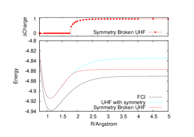
Figure 7: Unrestricted Hartree-Fock stretching of He${}_{2}^{+}$ compared with FCI. Shown at the top is the difference in charge between the two He atoms. FCI has $\Delta{\rm Charge=0}$ for all bond distances, however UHF incorrectly breaks the symmetry at around 1.8Å, with an incorrect smooth transfer of half an electron from one atom to the other.

Another system that shows up a qualitative problem of the UHF method is that of stretching of He${}_{2}^{+}$. Here, the problem is in symmetry breaking, as illustrated in Fig. 7. Infinitely stretched He${}_{2}^{+}$ with symmetry gives two He${}^{\frac{1}{2}+}$ atoms. UHF would give two high an energy due to its localization error (a concave behaviour of the energy for fractional systems). However, this too high energy is avoided by breaking the symmetry to give dissociation products of He and He⁺. This itself does not seem wrong, but the examination of the dissociation curve indicates that the symmetry breaking occurs at too short bond lengths, leading to an incorrect smooth transfer of electrons around 1.8 Å. Also the UHF curve falls off far too quickly compared to the FCI curve. This, of course, is very similar to the symmetry breaking in the spin densities seen in the UHF stretching of H${}_{2},$ which is often argued to be acceptable Perdew et al. (1995) as in H₂ the total density is not qualitatively wrong, whereas in the case of He${}_{2}^{+}$ it is incorrect. For He${}_{2}^{+},$ DFT methods such as UB3LYP dissociate with half an electron on each atom but give a completely wrong and much too low energy due to the delocalisation error. Similar symmetry breaking by UHF can be seen in many systems, for example Stein et al. (2014).

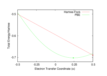
(a) The HZ^1e system with $Z=1.2$ for the wavefunctions $\Psi_{\alpha}=\sqrt{\left(\frac{1}{2}+\alpha\right)}\Psi_{(0)}+\sqrt{\left(\frac{1}{2}-\alpha\right)}\Psi_{(1)}$, with $-\frac{1}{2}\leq\alpha\leq\frac{1}{2}$. PBE incorrectly gives a minimum at $\alpha=0.24$, which corresponds to a qualitatively incorrect wavefunction with fractional charges on both atoms.

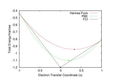
(b) HZ^{2e} with $Z=1.2$ along the electron transfer coordinate that moves both electrons from the H atom at $\alpha=-1$ to both electrons on the Z atom at $\alpha=1$. For $\alpha>0$, $\Psi_{\alpha}=\sqrt{(1-\alpha)}\Psi_{(0)}+\sqrt{\alpha}\Psi_{(1)}$, and $\alpha<0$ $\Psi_{\alpha}=\sqrt{(1-|\alpha|)}\Psi_{(0)}+\sqrt{|\alpha|}\Psi_{(2)}$. PBE and RHF both transfer fractional numbers of electrons because of the incorrect shape of their energy surfaces compared with the FCI energy surface for electron transfer.

Figure 8:

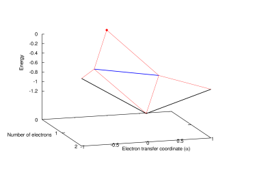
Figure 9: The total energy of HZ with $Z=1.2$ along the coordinate of transferring electrons for $0\leq N\leq 2$. The line in blue shows the energy at one electron and the line in black at two electrons, the red lines correspond to fractional number of electrons and are given by PPLB. The left hand side of the picture is when all the electron(s) are on the H atom and the right-hand side when all the electron(s) are on the Z atom.

V Fractional electron transfer coordinate

To understand in more detail the problem of the derivative discontinuity in HZ, let us consider the simplest case of HZ stretched to large distance (like 1000$a_{0}$). We now examine the transfer of electrons from one end of the molecule to another, in just one particular HZ system. In a single basis function per atom calculation this is very easy, as FCI gives just a trivial number of states. Let us first look at the system with one electron, where the FCI states are either one electron on the H, $\Psi_{{\rm H}}$ with energy $E_{{\rm H}}$, or one electron on the Z, $\Psi_{{\rm Z}}$ with energy $E_{{\rm Z}}$. Let us now consider a state that is a general coherent sum of these, $\Psi_{\alpha}=\sqrt{\alpha}\Psi_{{\rm H}}+\sqrt{(1-\alpha)}\Psi_{{\rm Z}}$, $0\leq\alpha\leq 1$. As $\Psi_{{\rm H}}$ and $\Psi_{{\rm Z}}$ are FCI wavefunctions (one is the ground state the other is the first excited state), they are orthogonal and eigenfunctions of the many-body Hamiltonian, so it is trivially obtained that $E[\Psi_{\alpha}]=\alpha E_{{\rm H}}+(1-\alpha)E_{{\rm Z}}$ and $\rho_{\alpha}(\mathbf{r})=\alpha\rho_{{\rm H}}(\mathbf{r})+(1-\alpha)\rho_{{\rm Z}}(\mathbf{r})$. This is very akin to fractional numbers of electrons as given PPLB (Eq. 5), such that when $\alpha$ is varied the energy varies linearly and the electron moves smoothly from the H to the Z. In contrast to PPLB all possible values of electron transfer, $\alpha$, correspond to an integer system with one electron and are represented by a wavefunction.

HZ with two electrons can be analyzed similarly. In this case, at the stretching limit, there are three singlet states with first order density matrices $\left(\begin{array}[]{cc}2&0\\ 0&0\end{array}\right)$, $\left(\begin{array}[]{cc}1&0\\ 0&1\end{array}\right)$ and $\left(\begin{array}[]{cc}0&0\\ 0&2\end{array}\right)$. The FCI wavefunctions that reduce down to give these density matrices are eigenfunctions of the Hamiltonian and orthogonal, so a linear combination of them will give a linear combination of both density matrices and energies. With more basis functions the idea is similar but the analysis more complex as there are many more possible states (one basis function excludes any excited states of the atoms).

Consider the case of HZ with $Z=1.2$ from FCI and compare it with a functional such as PBE, as shown in Fig. 8. First, for one electron (HZ^{1e}), where Hartree-Fock and FCI are equivalent, there is a straight line interpolation between the energies of the two atoms. Of course, a minimization of the FCI leads to one electron wholly on one side or the other, in this case the Z atom, as it is much lower in energy. The behavior of the energy with a functional such as PBE is qualitatively incorrect for one electron, as it does not have the correct linear straight line interpolation, but instead the energy varies smoothly (almost parabolically) with electron transfer. This leads to an incorrect minimum at around 0.26 electron on the H atom and 0.74 electron on the Z atom. The same result could be found with the compatible fractional calculations on each atom and piecing them back together, however, it is very good to see it in an integer electron system with a corresponding wavefunction. To summarise, in Fig. 8, PBE gives a good energy for the ground state $\Psi=\Psi^{(0)}$ (and also for the first excited state $\Psi=\Psi^{(1)})$ but incorrectly gives a much lower energy for a wavefunction $\Psi=\sqrt{0.74}\Psi^{(0)}+\sqrt{0.26}\Psi^{(1)}$.

For the two electron system (HZ${}^{\{2e\}})$, FCI has a minimum with one electron on each atom ($\Psi_{(0)})$ and two excited states, one with two electrons on the Z atom ($\Psi_{(1)})$ and the other with two electrons on the H atom ($\Psi_{(2)})$ . The straight line interpolations to be considered are between the ground state and first excited state and between the ground state and the second excited state. These are the lowest energy ones, a higher energy would be given by the interpolation between the first and second excited states. For any of these wavefunctions, the HF and PBE energies can be trivially evaluated from the density matrix, given that $T_{s}[\rho]$ for any two electron system is the von-Weisacker expression $T_{s}^{{\rm vW}}[\rho]=\int\frac{(\nabla\rho({\bf r}))^{2}}{8\rho({\bf r})}\mathrm{d}{\bf r}$. It is observed in Fig 8that both HF and PBE qualitatively fail to describe the electron transfer in this system. The energy on electron transfer is incorrectly smooth for both methods and with minima at the wrong values, HF at 0.33 electron on the H and 1.67 electron on the Z atom, and PBE with 0.4 electron on the H and 1.6 electron on the Z atom. In terms of the wavefunction, PBE is able to give a good energy for the excited states $\Psi=\Psi^{(1)}$ and $\Psi^{(2)}$, but due to its static correlation error PBE is unable to give a good energy for $\Psi=\Psi^{(0)}$. This means that PBE gives an incorrect minimum at $\Psi=\sqrt{0.4}\Psi^{(0)}+\sqrt{0.6}\Psi^{(1)}$. In general, density functional approximations favour an incorrect fractional charge transfer. Understanding all the possible states of this one systems is perhaps a much simpler challenge than understanding many different system (i.e. changing the molecule by changing $Z$) and yet captures the same physics.

VI Perspectives for the future

The key picture of the derivative discontinuity of the total energy is shown by FCI calculations in Figs 2 and 3, where the density increases smoothly but the energy is discontinuous on passing through one electron per site. Therefore, there is an intrinsic discontinuity in the exchange-correlation term that is a consequence of the particle nature of electrons. Approximate functionals in the literature completely miss this behaviour and the failure in the total energies is clear as, for example, in the qualitative breakdown to describe the energies of stretched H₂ and stretched H${}_{2}^{+}$. This error can be transformed into an error in the density as shown in the two electron example, HZ^{2e} (Fig. 5). This leads to qualitative failures to describe charge transfer, with an artificial bias to fractionally transfer electrons. Remarkably, this is seen in systems with integer number of electrons characterized by a wavefunction, in contrast to the delocalization error typical of fractionally charged systems.

It is clear that the problems caused by missing the derivative discontinuity are not just about stretching molecules, but it is the same physics that occurs in transition metal complexes, chemical reactions, or especially in electron transfer processes. Our hope is that the use of simple chemical model systems gives a more complete understanding of the nature of all types of electronic behaviour that occur in the intrincate nature of electronic structure.

The bumps of the exchange-correlation potential at the bond regions, where the density is very small, have been shown to have no effect on how electrons move and, therefore, do not capture the challenge of the derivative discontinuity. This illustrates the point that when the understanding appears quite paradoxical, it is just a clue that a deeper comprehension of the problem is needed.

We have highlighted the importance of the derivative discontinuity as a challenge for the energy functional at an integer number of electrons. We hope that understanding the examples given in this work can help highlight the avenue for development of new exchange-correlation functionals that contain the physics of the derivative discontinuity and represent the integer nature of electrons. This is needed so that DFT can play its role in helping tackle many important technological applications by correctly describing the movements of electrons in systems such as batteries and solar cells, chemical reactions in proteins, and transition metal compounds.