The host of the SN-less GRB 060505 in high resolution

Abstract

The spiral host galaxy of GRB 060505 at $z=0.089$ was the site of a puzzling long duration burst without an accompanying supernova. Studies of the burst environment by Thöne et al. (2008) suggested that this GRB came from the collapse of a massive star and that the GRB site was a region with properties different from the rest of the galaxy. We reobserved the galaxy in high spatial resolution using the VIMOS integral-field unit (IFU) at the VLT with a spaxel size of 0.67 arcsec. Furthermore, we use long slit high resolution data from HIRES/Keck at two different slit positions covering the GRB site, the center of the galaxy and an HII region next to the GRB region. We compare the properties of different HII regions in the galaxy with the GRB site and study the global and local kinematic properties of this galaxy. The resolved data show that the GRB site has the lowest metallicity in the galaxy with $\sim$1/3 Z_⊙, but its specific SFR (SSFR) of 7.4 M_⊙/yr/L/L* and age (determined by the H$\alpha$ EW) are similar to other HII regions in the host. The galaxy shows a gradient in metallicity and SSFR from the bulge to the outskirts as it is common for spiral galaxies. This gives further support to the theory that GRBs prefer regions of higher star-formation and lower metallicity, which, in S-type galaxies, are more easily found in the spiral arms than in the centre. Kinematic measurements of the galaxy do not show evidence for large perturbations but a minor merger in the past cannot be excluded. This study confirms the collapsar origin of GRB060505 but reveals that the properties of the HII region surrounding the GRB were not unique to that galaxy. Spatially resolved observations are key to know the implications and interpretations of unresolved GRB hosts observations at higher redshifts.

1 Introduction

GRB 060505 and its host galaxy have drawn particular attention in the GRB community for several reasons. GRB 060505 was one of two nearby long-duration GRBs that had no accompanying supernova (Fynbo et al., 2006; Gehrels et al., 2006; Della Valle et al., 2006; Gal-Yam et al., 2006). Due to its duration of only $\sim$ 4 s it was suggested that it could have intact been a short GRB that naturally has no SN (Ofek et al., 2007). However, the presence of a significant spectral lag (McBreen et al., 2008) and its afterglow properties (Xu et al., 2009) favour a long GRB origin. The host galaxy was somewhat unusual for a long-duration GRB, a late-type, moderately star-forming, solar metallicity spiral galaxy. Thöne et al. (2008), however, found that the properties of the stellar population at the GRB site very much resembled the global properties of dwarf GRB hosts (e.g. Christensen et al., 2004; Savaglio et al., 2009; Hjorth et al., 2012) concerning metallicity and star formation rate. Furthermore, it had a very young age, making the connection to a massive star even more likely.

GRB progenitor models suggest that long GRBs can only be produced by metal poor stars, otherwise, large mass losses of the massive progenitor slows down the star such that it cannot form an accretion disk at collapse (e.g. Woosley & Heger, 2006). Indeed, most long-duration GRBs have been found in metal poor environments or galaxies though a few exceptions for high metallicity environments have been found, e.g. GRB 020819 (Levesque et al., 2010a), GRB 050826 (Levesque et al., 2010b), GRB 080605 (Krühler et al., 2012) and GRB 090323 (Savaglio et al., 2012). Long duration GRB hosts furthermore show a moderate to high star formation rate. In the low redshift universe those conditions are mainly met in dwarf irregular and blue compact galaxies, but probably also in the outskirts of late-type galaxies. Short GRB hosts seem to show different properties (e.g. Berger, 2013) in line with the suggested origin in the coalescence of two compact objects.

In recent years, spatially resolved studies of GRB and SN hosts have become increasingly important. High spatial resolution imaging with the HST correlated the brightness in the blue at different parts in the host to the one at the explosion site. While SN Type II are distributed evenly, GRBs and Type Ic SNe are associated to the blues regions of their hosts (Fruchter et al., 2006; Kelly et al., 2008). Likewise, WC (cabon-oxygen Wolf-Rayet) stars show a spatial distribution similar to SNe Type Ic and GRBs concerning the brightness of their surrounding region while WN (nitrogen Wolf-Rayet) stars correlate with the distribution of SNe Ib (Leloudas et al., 2010). Short GRBs, in contrast, are found predominantly in dimmer regions and with larger offsets from their host galaxy, consistent with an older population and/or kicks of the progenitor system from the birth site by the preceding SN explosion (Fong et al., 2010).

Following the mass-metallicity relation, some more massive GRB hosts show a higher global metallicity of solar or supersolar values. However, most of them have actually a lower metallicity at the location of the GRB (Levesque et al., 2010a; Graham & Fruchter, 2013). As they are usually located in the outskirts of their hosts this is expected due to the usual metallicity gradient in star-forming galaxies. However, some GRB sites have still higher metallicities than theoretical models would require. GRB 0208019 (Levesque et al., 2010a) f.ex. showed a super-solar metallicity at the GRB site, however, it was a “dark GRB” (no optical counterpart was detected Jakobsson et al. (2005)). It is still debated weather the high metallicity might be the reason that those dark GRBs are intrinsically faint (see e.g. Graham & Fruchter, 2013) and whether we have to revise our theoretical models. The site of the short GRB 080905A (Rowlinson et al., 2010) in contrast showed an old population with little star formation, as expected.

Comparing GRBs and SNe, Modjaz et al. (2008) found a lower metallicity for GRB sites compared to broad-line Type Ic SNe without GRB. The situation is less clear for comparing different types of SNe, while Modjaz et al. (2011) finds a lower metallicities for Type Ib SNe compared to Type Ic, Anderson et al. (2010); Leloudas et al. (2011) do not see significant differences. Recent IFU studies of SN sites indeed show differences in metallicity, SFR and age between different types of SN (Kuncarayakti et al., 2013a, b; Galbany, 2013).

Detailed resolved studies using integral-field-spectroscopy has to date only been performed for the host of GRB 980425, the first GRB observed to be connected to a broad-line Type Ic SN (Christensen et al., 2008). The GRB site turned out to be not the youngest, most metal poor and star-forming region in the galaxy and did not show any WR features, in contrast to another star-forming region next to the one of the GRB site. This might imply that GRBs do not need the extreme properties as suggested by stellar population models and/or other evolutionary channels such as binaries might play an additional role. However, the sample of well studied GRB environment is still somewhat small to get some clear indications on the progenitors of these interesting events.

In this paper, we present integral field spectroscopic data of the host galaxy of GRB 060505 together with high resolution spectra in two slitpositions placed along the galaxy (Sec. 2). This allows us to study the properties of the different star-forming regions in the galaxy in terms of metallicity, star-formation rate, stellar population age and extinction and to compare the GRB region with other HII regions in the galaxy (Sec. 3). Furthermore, we investigate the kinematics of the galaxy to search for possible perturbations and other reasons for an increase in star-formation at the GRB site (Sec. 4).

2 Observations

Figure 1: Left panel: Image of the host galaxy of GRB 060505 in H$\alpha$. Middle panel: Positioning of the two HIRES slits overlaid on an image from HST/ACS in the F814W filter. Right panel: Contours of a FORS/VLT V-band image (same as in the following figures) and the different regions extracted as integrated spectra from the VIMOS datacube. The naming of the regions is used througout the paper. The site of the GRB is indicated with a cross or an arrow in the three panels, FOV in all three panels is $\sim$ 30”$\times$30”.

We obtained 9.85 h of observations with the integral field unit (IFU) of the VIMOS instrument at the VLT between April and August 2008. The setting with 0.67” lenslets and a 27” $\times$ 27” field-of-view (FOV) provides a sampling of $\sim$ 1 kpc and easily covers the entire galaxy with one pointing. The seeing conditions during most of the observations, however, were larger than 0$\aas@@fstack{\prime\prime}$7, reducing the resolution to 1$\aas@@fstack{\prime\prime}$34 or 2.2 kpc. Three different gratings were used, HR orange, HR blue and LR blue, to cover the wavelength range from 4000 to 7400 Å which includes all important diagnostic emission lines from [OII] to [NII]. The LR blue grating provides a resolution of $\lambda/\Delta\lambda$=250 whereas the HR orange and blue grism have resolutions of 2700 and 2600 respectively which barely resolves the emission lines.

The data were reduced and fluxcalibrated using the ESO VIMOS pipeline. The background was subtracted taking blank sections outside the galaxy in each of the four quadrants of the chip since they have slightly different readout noise and background levels. For each grism, all exposures were stacked to one single datacube and bad fibres masked out before the combination. The absolute flux calibration was scaled to match the broad-band magnitudes as listed in Thöne et al. (2008) using the integrated spectrum of the galaxy which also accounts for the large relative offset between the LRblue and the HR grisms. Fig. 1 shows an “image” of the galaxy summed in wavelength over the width of the H$\alpha$ line.

Furthermore, on July 16, 2007, we obtained two spectra with exposure times of 1800 and 1200s with HIRES and Keck I at the Keck Observatory on Mauna Kea, Hawaii. Using a 0$\aas@@fstack{\prime\prime}$8 slit, HIRES provides a spectral resolution of 45,000 or $\sim$ 7 km/s. With the red setting used, the orders almost overlap in the blue between 3990 and 4100 Å but this does not affect the [OII] emission lines present in this part of the spectrum. The HIRES slit has a length of 7” and was positioned at two different angles on the galaxy to cover the HII region at the GRB site, the center of the galaxy and another nearby HII region. The first position was chosen at the same angle (17 deg) as for the low-resolution spectra presented in Thöne et al. (2008), the second slit was positioned at zero degrees or North-South to cover the other large HII region west of the GRB position (see Fig.1).

The Keck/HIRES data were reduced using the HIRedux pipeline bundled within the XIDL software package. We used the pipeline to produce two-dimensional spectral images, calibrated in wavelength by tracing the ThAr lamp exposures. A rough estimate of the flux calibration was performed using the 1D spectra of spectrophotometric standard stars obtained on the same night. These do not account for slit losses but should provide good estimates ($\approx 10\%$) to the relative flux. Fig. 2 shows cut-outs of the 2D spectral images where $v=0$ km/s corresponds to the velocity recorded at the approximate center of the host galaxy. A significant shear in the velocity field is evident with increasing offset, indicating rotation of the galaxy.

Figure 2: Contour plots for H$\alpha$, [Oiii] and [Oii] along the two slit positions, left: along the major axis (slit 1), right: through the HII region next to the GRB site (slit 2). v=0 km/s corresponds roughly to the center of the galaxy. The color scale is a linear distribution of the pixel values for each individual line (not calibrated in absolute fluxes).

3 Resolved properties

The host of GRB 060505 is a low-mass (7.9$\times$10⁹ M_⊙), Sbc spiral galaxy seen almost face on with an inclination of 49 degrees (Thöne et al., 2008). The GRB happened in a star-forming (SF) knot in the northern spiral arm of the galaxy. As shown in Fig. 1, just west of the GRB region is another SF region (named “HII-N”). The host contains a number of other SF regions in the spiral arm to the south and west (HII-W) and south-west (HII-SW), south of the bulge (HII-S) and SF regions in the spiral arm to the east (HII-E). In the following, we apply the naming convention as marked in Fig. 1.

From the VIMOS/IFU data we create maps of emission lines and different properties across the host galaxy. To produce the emission lines maps we sum the flux of 15 pixels around the center of the corresponding emission line in each spaxel. The line continuum was subtracted taking the average of $\sim$10 pixels in the vicinity of the emission line free of other features. In the individual spaxels, only the LR blue grism shows some continuum emission due to its higher S/N per pixel. We furthermore extract integrated spectra for the different regions denoted in Fig. 1 and measure line-fluxes with standard tasks in IRAF, the integrated spectra are plotted in Fig. 3.

Figure 3: Integrated spectra of the different regions in the VIMOS dataset indicated in Fig. 1, offset by an arbitrary value for clarity. The spectra show all the three grisms used, the wavelength range was cutted in the overlapping wavelength regions and the fluxes scaled such as to exactly match the different spectra.

In the spectra of the individual spaxels we detect all of the strong emission lines of [OII], [OIII], H$\beta$, H$\alpha$ and [NII]. [SII] and H$\gamma$ are only detected in the integrated spectrum of the bulge, the [SII] doublet furthermore lies in a region of strong atmospheric emission lines and could therefore not be used. Line fluxes and properties of the integrated spectra are given in Tab. 1 and 2. A table with emission line fluxes and properties of all spaxels with fluxes of H$\alpha>$ 1.5$\times$10^-17 erg cm^-2 s^-1 can be found in Tab. 1 in the appendix.

The same lines were found in slit 1 of the HIRES data. Due to higher sensitivity in the red and high resolution the [SII] doublet is clearly detected here, albeit affected by atmospheric emission lines, and we also detect [NII] $\lambda$ 6548. For slit 2 we only see the [OII] doublet, [OIII] $\lambda$ 5007, H$\beta$ and H$\alpha$, [NII] $\lambda$ 6583 and [SII] $\lambda$ 6717 are very faint [NII] $\lambda$ 6548 and [SII] $\lambda$ 6731 are completely absent.

The longslit HIRES data are divided into spatial bins at a resolution similar to the seeing of around 0$\aas@@fstack{\prime\prime}$5, corresponding to a physical dimension of $\sim$ 0.8 kpc, from which we extract 1D spectra. We then fit Gaussian profiles to the emission lines in the extracted spectra, which represent a good fit to the emission lines in the individual spectra and determine their fluxes, center position and FWHM. The properties derived from this are found in Tab. LABEL:table:HIRESval in the appendix, due to the uncertainty in the absolute flux calibration of the HIRES data, we do not list the fluxes.

Region	[Oii]	H$\beta$	[Oiii]	[Oiii]	H$\alpha$	[Nii]	[Sii]	[Sii]
	$\lambda$3727/29	$\lambda$ 4862	$\lambda$ 4960	$\lambda$ 5008	$\lambda$ 6564	$\lambda$ 6585	$\lambda$ 6718	$\lambda$ 6732
GRB	2.39 $\pm$ 0.13	1.15 $\pm$ 0.07	0.76 $\pm$ 0.08	1.98 $\pm$ 0.06	3.11 $\pm$ 0.07	0.24 $\pm$ 0.03	1.75 $\pm$ 0.07	1.36 $\pm$ 0.47
HII-N	3.49 $\pm$ 0.25	0.78 $\pm$ 0.08	0.66 $\pm$ 0.07	1.93 $\pm$ 0.07	2.49 $\pm$ 0.05	0.70 $\pm$ 0.05	-0.20 $\pm$ -0.20	0.79 $\pm$ 0.22
HII-W	1.27 $\pm$ 0.42	1.01 $\pm$ 0.22	0.44 $\pm$ 0.04	1.34 $\pm$ 0.04	2.70 $\pm$ 0.06	0.46 $\pm$ 0.08	-0.20 $\pm$ -0.20	-0.20 $\pm$ -0.20
HII-SW	3.08 $\pm$ 0.50	1.56 $\pm$ 0.23	1.45 $\pm$ 0.13	2.83 $\pm$ 0.09	4.16 $\pm$ 0.10	0.35 $\pm$ 0.04	-0.20 $\pm$ -0.20	-0.20 $\pm$ -0.20
HII-S	1.14 $\pm$ 0.48	1.11 $\pm$ 0.48	0.39 $\pm$ 0.08	1.06 $\pm$ 0.06	1.57 $\pm$ 0.08	0.43 $\pm$ 0.04	-0.20 $\pm$ -0.20	-0.20 $\pm$ -0.20
HII-E	1.21 $\pm$ 0.31	1.16 $\pm$ 0.15	0.49 $\pm$ 0.20	0.88 $\pm$ 0.07	2.19 $\pm$ 0.09	0.19 $\pm$ 0.03	-0.20 $\pm$ -0.20	-0.20 $\pm$ -0.20
bulge	36.82 $\pm$ 4.06	8.86 $\pm$ 0.26	9.49 $\pm$ 0.35	16.30 $\pm$ 0.35	37.20 $\pm$ 0.91	9.18 $\pm$ 0.17	10.13 $\pm$ 0.36	9.78 $\pm$ 0.66
galaxy	61.92 $\pm$ 3.12	18.44 $\pm$ 0.73	12.98 $\pm$ 1.12	35.88 $\pm$ 1.44	77.10 $\pm$ 8.08	15.54 $\pm$ 1.63	20.28 $\pm$ 2.02	13.96 $\pm$ 3.78

Table 1: Fluxes measured in the integrated spectra of different regions in the VIMOS dataset in units of 10^-16 erg cm^-2 s^-1 (see Fig.1).

Region	12+log(O/H)	12+log(O/H)	log U	E(B–V)	SFR	SSFR	EW H$\alpha$
	(N2)	(O3N2)		[mag]	M⊙/yr	M⊙/yr/L/L*/spaxel	Å
GRB	8.23 $\pm$ 0.03	8.24 $\pm$ 0.00	-3.08 $\pm$ 0.04	0.00	0.047$\pm$ 0.001	7.43 $\pm$ 0.18	-57 $\pm$ 5.9
HII-N	8.49 $\pm$ 0.02	8.33 $\pm$ 0.01	-3.22 $\pm$ 0.05	0.14	0.038$\pm$ 0.001	7.37 $\pm$ 0.16	-130 $\pm$ 13.8
HII-W	8.39 $\pm$ 0.04	8.34 $\pm$ 0.01	-3.00 $\pm$ 0.16	0.00	0.041$\pm$ 0.001	6.88 $\pm$ 0.16	-83 $\pm$ 9.2
HII-SW	8.24 $\pm$ 0.03	8.25 $\pm$ 0.01	-3.05 $\pm$ 0.09	0.00	0.063$\pm$ 0.002	21.22 $\pm$ 0.51	-47 $\pm$ 5.4
HII-S	8.48 $\pm$ 0.03	8.42 $\pm$ 0.04	-3.04 $\pm$ 0.21	0.00	0.024$\pm$ 0.001	6.07 $\pm$ 0.32	-37 $\pm$ 5.0
HII-E	8.25 $\pm$ 0.04	8.33 $\pm$ 0.01	-3.13 $\pm$ 0.15	0.00	0.033$\pm$ 0.001	8.97 $\pm$ 0.38	-21 $\pm$ 3.9
bulge	8.46 $\pm$ 0.01	8.35 $\pm$ 0.01	-3.30 $\pm$ 0.06	0.40	0.566$\pm$ 0.014	4.36 $\pm$ 0.11	-38 $\pm$ 4.0
galaxy	8.42 $\pm$ 0.04	8.32 $\pm$ 0.01	-3.21 $\pm$ 0.04	0.40	1.173$\pm$ 0.123	6.49 $\pm$ 0.68	-62 $\pm$ 1.9

Table 2: Properties derived from integrated spectra in different regions in the VIMOS dataset (see Fig.1). Errors for the metallicity only includes the errors from the emission line fitting which are always smaller than the errors of the different calibrator (0.16 dex for the N2 and 0.18 dex for O3N2). log U is the ionization parameter obtained from [OII] to [OIII] as defined in Diaz et al. 2000.

3.1 Metallicity

The earlier longslit study on the host of GRB 060505 (Thöne et al., 2008) found a considerably lower metallicity (1/5 Z_⊙) at the site of the GRB compared to the other parts of the galaxy that have nearly solar values. With the VIMOS/IFU data we are now able to map the metallicity of the entire galaxy including the GRB site and determine whether the burst site is particularly metal poor or follows the general metallicity gradient in spiral galaxies (e.g. Henry & Worthey, 1999).

The metallicity is determined by the N2 and O3N2 indices using a recent recalibration by Marino et al. (2013) with systematic errors of 0.16 and 0.18 dex respectively: 12+log(O/H)$=$8.743 + 0.462  log₁₀(${\mathrm{[NII]6583}}/\mathrm{H\alpha}$) for the N2-index and 12+log(O/H)$=$8.533 – 0.214 log₁₀ ($\left(\mathrm{[OIII]5007}/\mathrm{H\beta})*(\mathrm{H\alpha}/{\mathrm{[NII]6583}})\right)$ for the O3N2 index. These indices are calibrated against metallicities derived from electron temperature measurements in nearby galaxies. For metallicities up to around solar values, those methods show a linear behaviour and are therefore a useful tool if direct measurements by the electron temperature are not available. Neither in the VIMOS nor in the HIRES data the temperature sensitive [OIII] $\lambda$ 4363 line is detected and we therefore have to rely on the indirect metallicity measurements. As solar metallicity we take 12+log(O/H)=8.69 (Asplund et al., 2009).

The maps for metallicities determined via the N2 and O3N2 indices are shown in Fig. 4 and 5. The VIMOS data give similar values for the metallicity determined from both methods. As expected in a star-forming spiral galaxy, there is a negative metallicity gradient from the centre to the spiral arms. Although the GRB region is the one with the lowest metallicity, similar values are reached in the SF regions in the SW spiral arm. The highest metallicities are actually not in the bulge but in a region just west of it. In the integrated spectra we get values of 12+log(O/H)$=$8.23 and 8.24 ($\sim$ 1/3 Z_⊙) from the N2 and O3N2 indices, somewhat higher than what has been previously determined from longslit data (Thöne et al., 2008). Again, the SW spiral arm has similar metallicities whereas the SF region (HII-N) next to the GRB region has somewhat higher metallicities. The bulge has higher metallicities but is still subsolar, somewhat lower than what had been found in the longslit data.

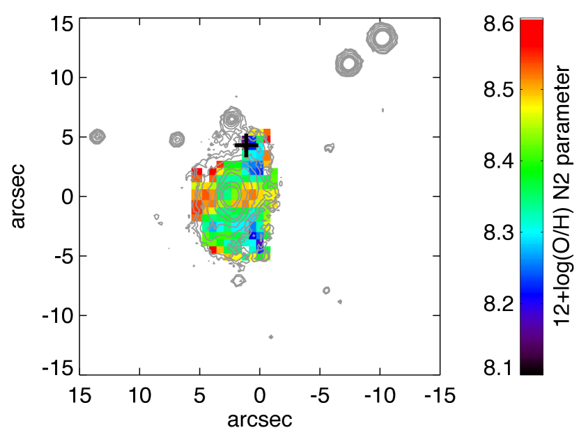
Figure 4: Metallicity map from the VIMOS data using the N2 index, as solar value we use 12+log(O/H)=8.69 (Asplund et al., 2009).

Figure 5: Metallicity map using the O3N2 index, as solar value we use 12+log(O/H)=8.69 (Asplund et al., 2009).

3.2 Ionization parameter

Regions with ongoing star-formation normally also have a higher ionization. The ionization of the medium is important for the determination of metallicity since the ionization influences the results in the metallicity, depending on the index used. Fig. 6 shows the ionization rate of oxygen in the galaxy using the parameter U defined in Diaz et al. (2000) as U$=$ –0.80 log([OII] 3726,29/[OIII] 5007) – 3.02. Due to the offset in the flux calibration between the LR blue and the HR orange grism (see Sect. 2), we use the fluxes for both lines measured in the LR blue grism

The variation in the ionization parameter is rather small across the galaxy both in the 2D datacube and the integrated regions. The star-forming generally show a somewhat higher ionization than the bulge, but nowhere [OIII] is particularly strong in comparison to [OII]. Ionization has been shown to correlate with metallicity, with ionization being higher at low metallicities (Dopita et al., 2006). The host of GRB 060505 follows more or less this trend, the places of lowest metallicity (GRB, HII-SW and HII-E) also have the highest ionization, although e.g. the ionization of HII-S with one of the highest metallicities is very similar to the one of the GRB site. Taking the ionization into account would imply metallicities of around 0.1 dex higher for the regions of higher ionization (see e.g. Kewley & Dopita (2002)) but no correction for the regions of lower ionization such as the bulge. We leave the values here without any correction for ionization.

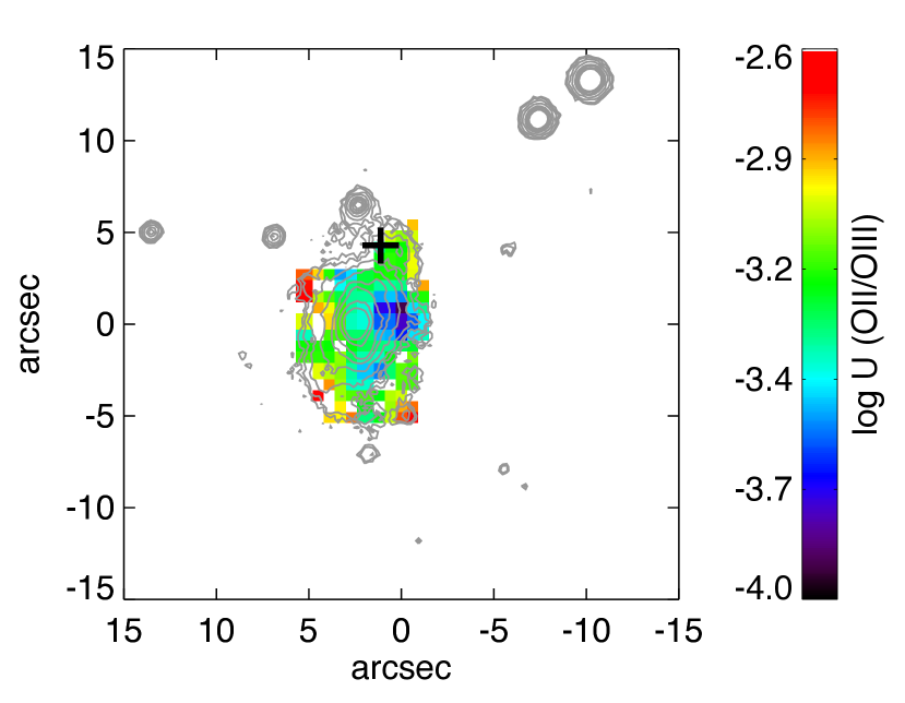
Figure 6: Ionization measured via the ratio of [OII] to [OIII]. We use the ionization parameter U defined in Diaz et al. (2000).

3.3 Star formation and age

To determine the star-formation rate we use the conversion between the H$\alpha$ emission line and the SFR as derived by Kennicutt (1998), $\mathrm{SFR}$[M_⊙/yr]=$7.9\times 10^{-42}4\pi f_{H\alpha}d_{L}^{2}$ with d_L being the luminosity distance. The H$\alpha$ emission is directly linked to the UV flux by young, massive stars and suffers relatively little from a possible extinction in the galaxy. The host has a total SFR of 1.2 M_⊙/yr, similar to the MW, but relatively high considering the low luminosity of $\sim$0.1 L* of the galaxy.

An estimate for the actual ongoing star-formation rate compared to the luminosity of the region is obtained by weighting the SFR with the B-band luminosity. We determine the B band magnitude by summing the flux in the B-band range from the LR blue grism data. The fluxes are converted to absolute magnitudes and we then multiply the SFR with the ratio between the absolute magnitudes and the magnitude of an L* galaxy M${}_{\mathrm{B}}=$-21 mag in order to obtain the specific (luminosity-weighted) star-formation rate (SSFR) using the following conversion: $\mathrm{SSFR}$=$\mathrm{SFR}\times 10^{0.4(M_{B}+21.)}$. The values for the integrated spectra are then normalized to the value per spaxel to account for the different sizes of the extracted regions.

While the SSFR generally indicates a somewhat elevated SF throughout the galaxy, the SSFR increases from the centre to the spiral arms of the galaxy as it is expected for an inside-out starformation scenario in spiral galaxies. The highest SSFR is found in the SW-spiral arm that is also very prominent in the H$\alpha$ image of the galaxy while the rest of the HII regions show similar values for the SSFR. The SSFR follows the same trend as found in the longslit data of Thöne et al. (2008) albeit it is less pronounced as found in the previous work.

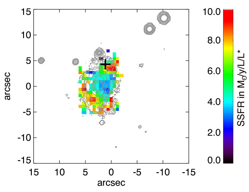
Figure 7: SFR weighted by the restframe B-band luminosity in M_⊙/yr/kpc/L/L*, the cross indicates the region of the GRB.

As a rough proxy for the age of the stellar population, we use the equivalent width (EW) of H$\alpha$. We can only do this for the integrated regions since the continuum is generally too weak in the individual spaxels. Surprisingly, the EW is not high in all of the star-forming regions. The GRB site only has the third highest EW after the HII-N next to the GRB site and HII-W, which has otherwise no extreme properties. In Thöne et al. (2008) an EW of almost -200Å was found (corresponding to an age of $\sim$6Myr), considerably higher than in the other parts of the galaxy along the slit. This difference to the longslit data might be explained by integrating over larger regions comprising parts with lower EWs than it was done for the longslit data, which had been obtained under good seeing conditions of 0.75 arcsec (Thöne et al., 2008).

3.4 Extinction

We determined the extinction in each spaxel by using the Balmer line decrement H$\alpha$/H$\beta$ which has a fixed value of 2.76 for case B recombination and zero extinction (Osterbrock, 1989). Regions with a H$\beta$ flux of less than 0.1$\times$10^-16 erg cm² s^-1 were excluded from the extinction measurements.

The extinction is low or consistent with zero throughout most regions of the galaxy including the GRB site. Only the bulge shows some extinction, which primarily comes from some more dusty region in the southern part of the bulge. It has already been noted in Thöne et al. (2008) that the low extinction excludes that a possible SN to GRB 060505 was hidden by dust. It also implies that the SFR we see is not severely affected by dust and can be taken as close to the absolute SFR in the galaxy. Due to the low extinction in most parts of the galaxy, we do not correct the emission line fluxes for extinction.

Figure 8: Extinction values in E(B–V) using the Balmer decrement of H$\alpha$ vs. H$\beta$, regions with H$\alpha$ $<$ 0.15$\times$10¹⁶erg cm^-2 s^-1 were excluded.

3.5 Comparison between different HII regions

One of the main intentions of the paper is to investigate whether the GRB region had unique properties or whether it was a mere coincidence that the GRB occurred exactly in this SF region. Furthermore, we want to study if the global properties of the galaxy are largely different from the properties of the GRB site as we would have measured it for the same galaxy at a higher redshift. This in turn would then give wrong conclusions for similar cases where the host galaxy had been at higher redshift and unresolved.

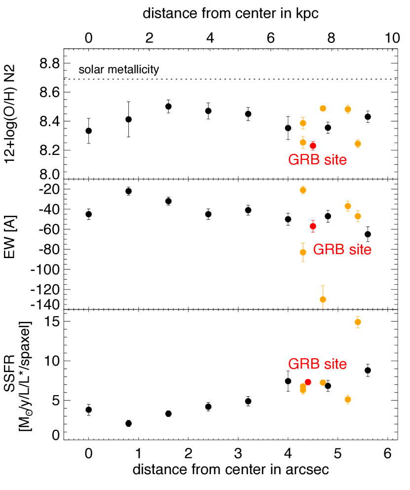
Figure 9: Comparison of different properties between the integrated HII regions as show in Fig. 1 (orange points) and the average properties extracted from elliptical regions around the center of the galaxy (black points). The HII regions are plotted at their corresponding deprojected distance from the galaxy centre. The integrated spectrum of the bulge was left out in the plot. For the EW we used the H$\alpha$ line.

We compare the different HII regions with the average properties at their corresponding distance from the centre. To do this, we extract integrated spectra of ellipses around the centre in steps of 0$\aas@@fstack{\prime\prime}$8 using a PA of 38 deg and an inclination of 49 deg (see Thöne et al. (2008)). The properties from these elliptical regions are determined in the same way as for the integrated regions and the results for both the ellipses and the HII regions at their corresponding deprojected distance are plotted in Fig. 9. Fluxes and derived values for the ellipses are found in Tab.3 and Tab.4 in the appendix.

The metallicity shows an initial rise and then follows a slight gradient towards the outskirts. The inverse is the case with the EW, indicating a somewhat younger population in the outskirts. The SSFR/spaxel is low in the bulge and rises towards the outskirts. The SSFR of all but one HII region, including the GRB site, is around the average at that distance from the centre, not surprising, since it is exactly those HII regions that contribute to the SFR in the spiral arms. The GRB site is only somewhat different from the average value at its distance from the centre in the metallicity and the SSFR while it has an “average” EW and hence age. Except for the EW, the GRB region has the most extreme properties in the galaxy but is not a stark outlier as suggested in the longslit data in Thöne et al. (2008). The other HII regions are rather scattered in their properties, but all have rather high SSFRs compared to their position in the galaxy, not surprising since they were defined as such by their large H$\alpha$ fluxes.

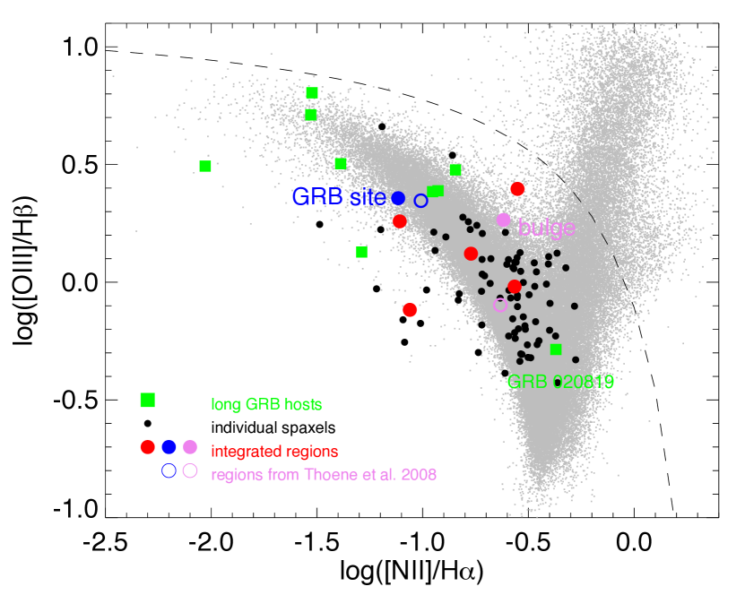
Figure 10: BPT diagram of NII/H$\alpha$. In grey are emission line galaxies from the SDSS DR 10, green are other z$<$0.5 long GRB hosts, most of them are data from unresolved hosts. Black dots represent individual, filled circles integrated regions in the host of GRB 060505 from the VIMOS data. The dashed line is the dividing line between AGN and HII regions as derived in Kewley et al. 2006. For comparison, we also show the line ratios of the GRB site and the bulge as derived from the longslit data on the host from Thöne et al. 2008 (blue and purple empty circles).

We put the values from the integrated regions as well as individual spaxels in the “Baldwin, Philips and Terlevich” diagram (Fig.10) where we plot [NII]/H$\alpha$ vs. [OIII]/H$\beta$, which are also used for determining metallicities (see Sect. 3.1). This diagram allows to distinguish between region excited by radiation from young stars and such excited by AGNs. All regions in our host are clearly not affected by any AGN activity. The diagram furthermore gives some indications of metallicity and age with metallicity decreasing towards the left (since [NII]/H$\alpha$ is a metallicity calibrator) and the age increasing from top to bottom. The GRB site is hence one of the more metal poor and younger regions in the host but not as extreme as a number of other long duration GRB hosts.

An important issue when making any conclusions on the progenitor from measurements of the GRBs environment or host is the spatial resolution. Depending on the size of the probed region and how properties vary across the host determine how accurately the measurement at the “GRB site” reflect the actual environment. In order to test this, we rebin the datacube of the GRB 060505 host to resolutions the VIMOS data would have given us if the host had been at z$=$ 0.2 and 0.53 and compare it with the values of the original datacube (see Fig. 11). Any decrease in resolution generally wipes out locally confined more extreme properties. The metallicity gradient becomes much shallower and any difference between the HII regions around the centre basically disappears.

The conclusions derived from longslit data on the other hand crucially depend on the placement of the slit. In our case the GRB region was sticking out in its properties compared to the other parts probed along the slit and also compared to the HII region at the opposite arm. This is a chance coincidence since we probed the tip of the HII-S region which actually has the highest metallicity among the HII regions. Regions similar to the GRB site like the bright HII-SW region were completely missed as would have been any HII region outside the slit with properties very different from the GRB site. By placing a longslit through the centre of a barely resolved large host at high redshift could have a similar effect since a significant fraction of the HII regions in the spiral arms would be missed in the spectrum and the analysis.

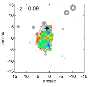
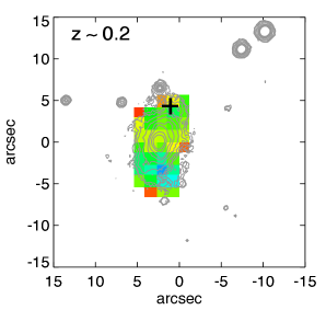
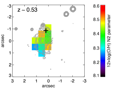
Figure 11: Simulation of the metallicity (N2 index) distribution in the host if the galaxy had been at redshifts of z$\sim$0.2 and 0.53, in comparison to the actual position at z$=$0.09. The color scale varies slightly between the different plots for better visualization of the metallicity scale. The data have only been rebinned, lower S/N due to the larger distance was not taken into account.

3.6 Analysis of the HIRES data

The HIRES data allow us to study the metallicity, extinction and [SII]/H$\alpha$ along slit 1 which goes from the centre of the galaxy to the GRB site. For slit 2, [NII] and [SII] are too weak to be fitted and we can therefore only derive the ionization and extinction but no metallicity.

Concerning the metallicity, the HIRES data give consistent values for the N2 and the O3N2 index. We can only determine the metallicity just before the GRB site since [NII] is not detected with high enough significance at the GRB site whereas H$\alpha$ is clearly visible, which further points to a low metallicity. The metallicity just next to the GRB region is 0.1 dex higher than the values found in the integrated spectrum of the GRB site from the VIMOS data. The metallicity gradient shows the same behaviour as for the VIMOS integrated spectra at different distances from the centre reaching the highest value at the outskirts of the bulge, not in the centre, and subsequently falling towards the outskirts.

Due to the better resolution allowing a better skyline subtraction, we can determine the ratio log ([SII]$\lambda$ 6717,6731/H$\alpha$) along slit 1 in the HIRES data. [SII]$\lambda$ 6731 has too low S/N for a proper extraction and the ratio of the two SII lines can generally vary between $\sim$ 1.5 for low electron density and $\sim$0.5 for high densities. From the longslit data we know that [SII] 6717/ [SII] 6731 is always $>$1.25 and we therefore take a ratio of 1.3 for all the regions, hence the values for [SII]/H$\alpha$ are hence considered a lower limit. log([SII]/H$\alpha$) has values similar to what has been found in nearby spiral galaxies and there is no indication for regions excited by shocks which would give ratios of [SII]/H$\alpha$ around 1. The extinction along both slits is very low or not measurable basically along all the slit, consistent with what we found for the VIMOS data.

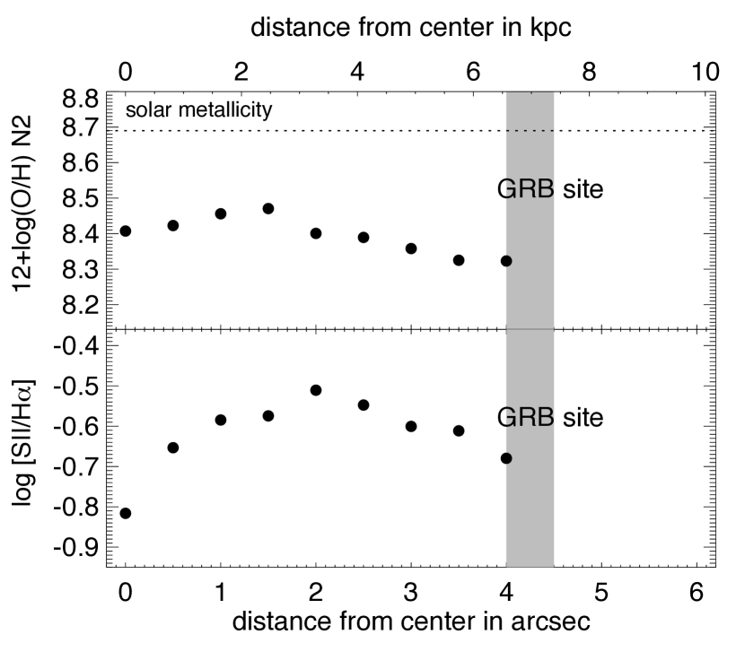
Figure 12: Metallicity and [SII]/H$\alpha$ along slit 1 of the HIRES data. The values are listed in Tab.LABEL:table:HIRESval in the appendix.

4 Kinematics of the galaxy

The host of GRB 060505 is an isolated dwarf spiral with no obvious signs of interaction. The large-scale environment confirms that it does not belong to a larger group, but it might be part of a filament extending from the Abell 3837 cluster (Thöne et al., 2008). Interaction has been one possible cause for an increase in star-formation which again facilitates the formation of very massive stars and hence GRBs, but SF can also be triggered by gas inflow or compression due to supernova explosions. In the following, we investigate the resolved kinematics of our galaxy to check for external causes for the recent star-formation.

4.1 Rotation curve fitting

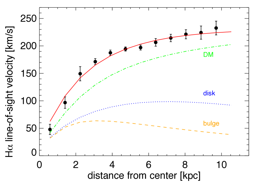
Figure 13: Rotation curve for one half of the GRB 060505 host using the H$\alpha$ line of slit 1 of the HIRES spectra corrected for the inclination of 49deg. We fit the rotation curve with disk, bulge and a DM halo component, as DM halo profile we used an isothermal sphere. The velocities of H$\alpha$ are listed in Tab.LABEL:table:HIRESval in the appendix.

In Thöne et al. (2008) we derived a rotation curve using H$\alpha$ from low-resolution longslit data. Here we improve the analysis by using the high-resolution longslit data from the HIRES spectrograph which cover the region roughly from the centre or the galaxy to just beyond the GRB region. We take the strongest emission line, H$\alpha$ and extract the line profiles for each bin along the spatial direction where one bin corresponds to one row in the spectrum which is 0.5 arcsec or 0.8 kpc. These profiles are then fit by Gaussians, the centers of which are plotted in Fig. 13, corrected for the inclination of 49 deg (Thöne et al., 2008).

We then fit this rotation curve with contributions from the disk, the bulge and a dark matter (DM) halo where we take the DM-profile of an isothermal sphere. Other DM profiles would only be different in the outermost regions which we cannot probe with the strong emission lines from SF regions. We get a best fit with the following values ($\chi^{2}$ = 9.4 with 6 d.o.f): a disk scale length of 8.2$\pm$1.6 kpc, a mass-to-light ratio of 6.8$\pm$1.3 (solar units), a central luminosity density of 59.8$\pm$11.4$\times$10^-3M_⊙/pc³, a DM core radius of 2.8$\pm$0.3 kpc and a central density of the DM halo of 144$\pm$35$\times$10^-3 M_⊙/pc³ and a bulge radius of 2.3$\pm$0.3 kpc.

The rotation curve does not show any obvious particularities, only the fit in the innermost few kpc is not very good as the rotation curve rises steeper than expected. A steep rise has been observed in a number of spiral galaxies, especially when they have massive bulges (e.g. Sofue & Rubin, 2001, and references therein). The data quality, however, is too poor make any firm conclusion on a possible additional component or a high mass concentration in the center.

4.2 Velocity map and dispersion

We plot the 2D velocity map from the VIMOS data by fitting the [OIII] emission line with a gaussian fit for all spaxels where the line is detected with large enough significance. [OIII] was used instead of the somewhat stronger H$\alpha$ line due to problems in the shape of H$\alpha$ in a few spaxels in the center of the galaxy, which is probably due to bad pixels. In Fig. 14, we plot the velocity of the line center taking the center of the galaxy (z=0.0901) as 0 km s^-1. We further analyze the line width in the radial direction from the two slits of the HIRES data using the strongest lines H$\alpha$ and [OIII] plotted in Fig.15.

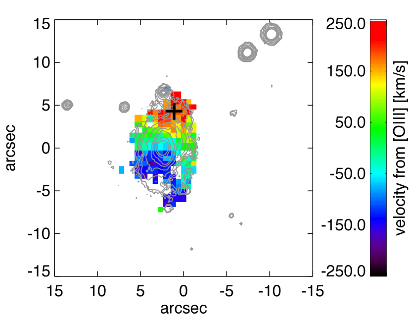
Figure 14: Velocity map determined from the center and FWHM of the [OIII] emission line in the VIMOS data.

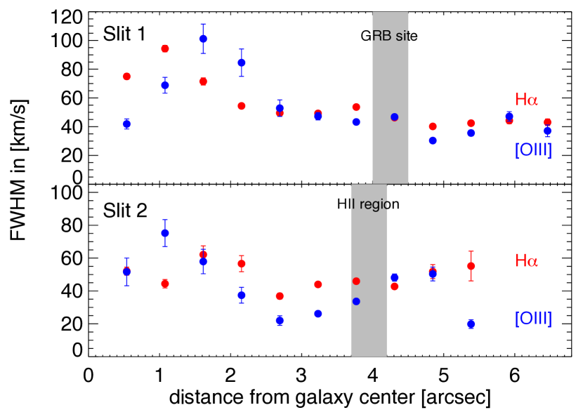
Figure 15: Velocity dispersion along the two slits for H$\alpha$ and [OIII], slit 1 includes the GRB region, slit 2 the HII regions next to it (HII-N following the naming in the VIMOS data). The shaded lines indicate the position of the GRB region and the HII region next to it respectively. The values are listed in Tab.LABEL:table:HIRESval in the appendix.

The velocity field is rather homogeneous at first glance showing a regular rotating disk. We will investigate this further in the next chapter. The FWHM of the emission lines is around 100 km s^-1 in the centre and decreases outwards towards the spiral arms as seen in the radial HIRES slit (slit 1). An enhancement in the central line width is an indication for gas infall forming a bulge whereas very young disk galaxies show essentially a flat velocity dispersion along the axis (for a small overview over spiral galaxy rotation curves and velocity dispersions see Beckman et al., 2004). The line width falls rapidly and remains constant at about the same distance from the center where the rotation curve starts to flatten which is also what we observe here. The difference in velocity between the centre and the spiral arms suggests that the bulge is not very large as is the case in more evolved spiral galaxies.

4.3 Kinemetry analysis

We further analyze the kinematics of the galaxy by fitting the velocity map with kinemetry models as detailed in Krajnović et al. (2006). The method derives kinematical information by fitting ellipses to the velocity map described by a harmonic expansion. Higher order moments of the expansion give an indication of perturbed velocity fields. The best fit ellipses overplotted on the velocity map as well values for the PA, ellipticity and the coefficients k1 and k5 of the harmonic expansion are shown in Fig.16.

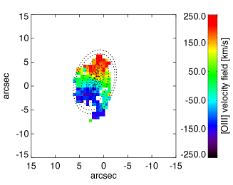
Figure 16: Top part: Best fit kinemetry ellipses overplotted on the velocity map derived from [OIII]. Bottom part: Best fit parameters at the different positions relative to the centre of the galaxy. $\Gamma$ is the PA, q the flattening parameter or ellipticity, k1 is the dominant coefficient of odd kinematic moments and indicates the amplitude of the bulk motion for velocity maps. k5/k1 is a measure for the deviation from simple rotation since k5 is the first higher-order term only present in case of perturbations from normal rotation.

Our galaxy overall has an axisymmetric velocity field, the PA of the best fit ellipses remains constant across the galaxy and k1 is identical with the rotation curve of the galaxy. The flattening or ellipticity parameter q changes its value at around 4 arcsec which could be indicative of a separate component in the inner parts of the galaxy, but the data are not good enough for a definite conclusion. The jump in q in the third fitted ellipses is due to an anomaly in the data and likely not real. The ratio k5/k1 is indicative of deviations from simple rotation in the map and overall rather low but still not negligible. The higher value in the outskirts could point to some perturbations that created the large SF region such as the one to the SW, but at this point we cannot exclude that these deviations are purely a result of the relatively low data quality for this kind of analysis.

Kinemetry has mostly been used for nearby galaxies, although comparisons with model galaxies allowed to distinguish between mergers and unperturbed systems at z$\sim$2 Shapiro et al. (2008) with even lower spatial resolution and data quality. According to the classification in this paper using the asymmetry in the velocity and dispersion map derived from the coefficients of the harmonic expansion v_asym vs $\sigma_{asym}$ our galaxy lies in the transition between unperturbed galaxies and mergers. This could be an indication that the SF in this galaxy might be somehow related to some merger event in the past.

5 Discussion and conclusion

The host of GRB 060505 was only the second GRB host that has been studied with IFU spectroscopy. It had also the second lowest redshift ever measured for a GRB, making it a fortunate case to study the host in detail, which is currently not possible for the majority of GRB hosts. Studies like the one presented here are crucial to determine the validity of future resolved host studies at higher redshift. GRB hosts at low redshift have proven to be a very mixed bag of galaxies, probably because those bursts would go undetected at higher redshifts. This makes it even more important to carefully study those hosts in detail and to investigate possible biases.

The earlier study with a longslit across the major axis of the galaxy presented in Thöne et al. (2008) suggested that the GRB site is a region with rather peculiar properties compared to the rest of the galaxy. Our new study shows that most of the star-forming regions in that galaxy around the bulge in various spiral arms have similar properties to the GRB site and the strong conclusion was mainly an issue of the longslit placement. The GRB site, however, does have the lowest metallicity (albeit within errors) in the host galaxy.

The kinematic analysis shows a rather smooth velocity field and rotation curve. The high dispersion in the centre might point to some gas inflow to an existing yet not very evolved bulge. A thorough kinemetric analysis reveals some degree of disturbance in the velocity field and we cannot exclude some minor merger event in the past. The host overall has no really extreme properties and the SF in the region around the GRB could simply be due to the inside-out SF propagation usually observed in spiral galaxies.

Our analysis shows the importance to study low redshift GRB hosts with spatially resolved techniques to be able to properly interpret the global spectra of the entire galaxy that we have to deal with for the large majority of GRB hosts. GRB host are mostly dwarf galaxies, nevertheless they can have different properties throughout the host which is even more relevant for larger hosts. Steep metallicity gradients can lead to wrong metallicities at the GRB site since they are usually found in the outskirts of their hosts, f.ex. determining the metallicity of the integrated spectrum in a larger host seen edge on where the GRB is seemingly lies at the brightest spot of the galaxy but in reality is found in some outer spiral arm (in front or even behind the galaxy since GRBs easily outshine their hosts) would lead to a wrong value.

Integral field studies of galaxies at all redshifts have become an extremely growing field. Several past and ongoing large IFU such as CALIFA (Sánchez et al., 2012) or VENGA (Blanc et al., 2013) have revealed a lot of information about the gas properties and star-formation history in different kinds of galaxies, but so far they target large nearby galaxies different from the host of GRB 060505 and most other GRB hosts. With future large IFU surveys such as MANGA we might even be lucky to observe a galaxy before and after it hosted a GRB to determine if and how such a large explosion influences its immediate environment.

Table 3: Fluxes and various properties from the VIMOS data. Fluxes are in 10^-16 erg cm^-2 s^-1.

Spaxel	H$\alpha$	H$\beta$	[NII]	[OIII]	[OII]	Z (N2)	Z (O3N2)	log U	SSFR	E(B–V)
			6586	5007	3727,29	12+log(O/H)	12+log(O/H)	[OII]/[OIII]	M⊙/yr/L/L*	[mag]
20 11	0.15	0.02	0.00	0.08	0.68	0.00	8.44	-2.87	5.29	0.00
21 11	0.15	0.02	0.00	0.06	0.84	0.00	8.54	-3.31	7.60	0.00
19 12	0.18	0.06	0.01	0.05	0.20	8.32	8.42	-2.78	6.94	0.00
20 12	0.27	0.06	0.00	0.07	0.57	8.03	8.30	-2.98	11.25	0.00
21 12	0.25	0.05	0.00	0.06	0.65	8.03	8.35	-3.15	11.93	0.06
22 12	0.16	0.04	0.00	0.07	0.68	0.00	8.39	-3.24	10.67	0.00
19 13	0.22	0.07	0.02	0.07	0.19	8.23	8.43	-3.43	8.87	0.00
20 13	0.31	0.06	0.03	0.08	0.44	7.97	8.23	-3.32	12.36	0.00
21 13	0.27	0.05	0.00	0.09	0.48	0.00	8.14	-3.32	12.40	0.08
22 13	0.18	0.04	0.00	0.10	0.66	0.00	8.24	-3.13	10.15	0.00
18 14	0.16	0.03	0.03	0.04	0.34	8.57	8.47	-2.82	7.93	0.04
19 14	0.17	0.06	0.00	0.09	0.21	0.00	8.42	-3.31	8.42	0.05
20 14	0.26	0.06	0.00	0.12	0.36	8.14	8.24	-3.20	12.46	0.06
21 14	0.25	0.06	0.00	0.14	0.25	0.00	8.25	-3.01	11.49	0.00
22 14	0.24	0.06	0.00	0.15	0.53	0.00	8.25	-2.79	13.19	0.00
23 14	0.16	0.07	0.00	0.14	0.53	0.00	8.45	-2.69	8.61	0.00
13 15	0.15	0.06	0.03	0.04	0.21	8.25	8.34	-3.18	7.21	0.00
17 15	0.19	0.03	0.07	0.05	0.28	8.52	8.48	-2.94	8.30	0.18
18 15	0.23	0.05	0.04	0.10	0.40	8.48	8.43	-2.83	8.75	0.26
19 15	0.20	0.06	0.00	0.14	0.48	0.00	8.38	-3.22	8.67	0.19
20 15	0.25	0.06	0.02	0.17	0.49	7.96	8.25	-3.16	10.45	0.25
21 15	0.23	0.05	0.00	0.16	0.47	0.00	8.18	-3.05	9.80	0.00
22 15	0.23	0.07	0.00	0.13	0.63	0.00	8.17	-2.88	10.59	0.03
23 15	0.17	0.08	0.00	0.10	0.80	0.00	8.18	-2.82	6.76	0.00
13 16	0.17	0.03	0.02	0.03	0.24	8.25	8.35	-3.24	8.13	0.00
15 16	0.23	0.07	0.04	0.00	0.14	8.51	8.35	-2.66	7.63	0.00
16 16	0.23	0.06	0.03	0.01	0.21	8.50	8.45	-2.78	5.58	0.33
17 16	0.29	0.06	0.02	0.06	0.42	8.47	8.49	-3.05	6.51	0.25
18 16	0.28	0.07	0.03	0.12	2.26	8.44	8.44	-3.12	7.50	0.41
19 16	0.22	0.06	0.00	0.16	2.42	0.00	8.39	-3.14	7.05	0.31
20 16	0.21	0.06	0.00	0.19	2.50	0.00	8.25	-3.21	8.35	0.34
21 16	0.19	0.06	0.00	0.17	0.78	0.00	8.14	-3.03	7.34	0.09
22 16	0.21	0.08	0.00	0.18	0.74	0.00	8.13	-3.00	8.73	0.17
23 16	0.22	0.07	0.00	0.11	0.72	8.28	8.18	-3.08	8.51	0.03
13 17	0.15	0.02	0.00	0.04	0.47	0.00	8.31	-3.19	6.21	0.00
14 17	0.17	0.05	0.00	0.04	0.38	0.00	8.25	-2.97	7.33	0.00
15 17	0.29	0.07	0.06	0.03	0.40	8.37	8.29	-2.82	9.03	0.00
16 17	0.37	0.07	0.05	0.07	0.55	8.40	8.32	-2.85	8.22	0.25
17 17	0.41	0.08	0.08	0.13	0.78	8.40	8.40	-3.05	7.84	0.24
18 17	0.38	0.09	0.08	0.20	4.17	8.40	8.42	-3.38	6.75	0.40
19 17	0.31	0.09	0.04	0.20	3.72	8.36	8.40	-3.39	6.64	0.40
20 17	0.27	0.09	0.02	0.19	3.66	8.31	8.35	-3.48	6.41	0.24
21 17	0.24	0.08	0.00	0.13	0.31	0.00	8.22	-3.14	6.89	0.00
22 17	0.22	0.11	0.01	0.15	0.75	8.27	8.27	-3.12	8.53	0.00
23 17	0.21	0.09	0.04	0.10	0.60	8.36	8.31	-3.13	10.40	0.00
14 18	0.18	0.08	0.01	0.06	0.33	8.36	8.39	-3.01	6.86	0.27
15 18	0.35	0.12	0.04	0.09	0.53	8.37	8.35	-2.98	8.18	0.18
16 18	0.54	0.12	0.05	0.14	0.86	8.43	8.30	-3.02	8.89	0.30
17 18	0.67	0.12	0.09	0.19	1.20	8.44	8.31	-3.07	9.12	0.24
18 18	0.60	0.10	0.09	0.23	4.74	8.45	8.34	-3.35	7.95	0.39
19 18	0.46	0.08	0.04	0.19	4.26	8.41	8.32	-3.49	6.07	0.39
20 18	0.32	0.10	0.02	0.16	4.21	8.36	8.34	-3.56	4.61	0.34
21 18	0.26	0.09	0.00	0.12	0.69	0.00	8.31	-3.30	4.96	0.06
22 18	0.23	0.10	0.01	0.16	0.93	8.39	8.39	-3.11	9.56	0.17
23 18	0.24	0.07	0.06	0.13	0.66	8.48	8.46	-3.15	12.77	0.00
24 18	0.20	0.05	0.08	0.08	0.57	8.58	8.52	-3.10	11.79	0.00
14 19	0.21	0.10	0.02	0.07	0.28	8.39	8.41	-3.15	7.63	0.00
15 19	0.36	0.16	0.06	0.16	0.60	8.43	8.38	-3.16	7.87	0.00
16 19	0.53	0.17	0.08	0.24	1.12	8.46	8.34	-3.17	8.11	0.15
17 19	0.68	0.17	0.12	0.26	1.60	8.46	8.31	-3.06	7.64	0.21
18 19	0.67	0.15	0.13	0.28	3.52	8.48	8.31	-3.28	6.24	0.44
19 19	0.63	0.13	0.14	0.26	3.00	8.47	8.29	-3.36	5.00	0.45
20 19	0.49	0.12	0.09	0.24	2.91	8.45	8.35	-3.38	4.16	0.43
21 19	0.36	0.09	0.03	0.20	1.08	8.40	8.36	-3.20	4.29	0.25
22 19	0.28	0.09	0.04	0.19	1.25	8.44	8.43	-3.15	8.86	0.33
23 19	0.27	0.07	0.08	0.16	0.92	8.52	8.46	-3.09	14.10	0.12
24 19	0.24	0.06	0.10	0.10	0.79	8.65	8.51	-3.04	14.02	0.00
12 20	0.17	0.04	0.01	0.04	0.69	8.17	8.50	-3.05	8.36	0.00
13 20	0.16	0.06	0.01	0.03	0.68	8.39	8.48	-3.14	7.20	0.00
14 20	0.21	0.10	0.07	0.04	0.78	8.51	8.44	-3.19	7.78	0.00
15 20	0.33	0.14	0.12	0.13	0.61	8.56	8.42	-3.17	5.96	0.00
16 20	0.46	0.16	0.11	0.21	1.08	8.55	8.38	-3.19	5.83	0.15
17 20	0.70	0.18	0.15	0.24	1.59	8.52	8.30	-3.15	6.25	0.22
18 20	0.77	0.19	0.16	0.27	2.03	8.54	8.31	-3.21	5.17	0.38
19 20	0.83	0.18	0.25	0.28	2.18	8.56	8.32	-3.28	4.25	0.48
20 20	0.68	0.15	0.20	0.29	2.32	8.55	8.37	-3.32	3.51	0.42
21 20	0.48	0.09	0.11	0.25	2.19	8.51	8.36	-3.34	3.07	0.23
22 20	0.32	0.06	0.04	0.24	1.72	8.51	8.42	-3.27	6.07	0.29

Table 1: continued.

Spaxel	H$\alpha$	H$\beta$	[NII]	[OIII]	[OII]	Z (N2)	Z (O3N2)	log U	SSFR	E(B–V)
			6586	5007	3727,29	12+log(O/H)	12+log(O/H)	[OII]/[OIII]	M⊙/yr/L/L*	[mag]
23 20	0.27	0.05	0.07	0.23	1.23	8.57	8.44	-3.24	10.33	0.21
24 20	0.26	0.05	0.10	0.16	0.95	8.63	8.51	-3.10	12.76	0.00
25 20	0.19	0.06	0.08	0.10	0.91	8.67	8.47	-3.08	10.85	0.00
13 21	0.16	0.05	0.00	0.03	0.61	0.00	8.55	-3.32	8.09	0.00
14 21	0.20	0.06	0.07	0.02	0.72	8.59	8.41	-3.38	9.46	0.00
15 21	0.30	0.09	0.13	0.08	0.39	8.64	8.40	-3.17	7.96	0.00
16 21	0.42	0.13	0.15	0.17	0.95	8.61	8.40	-3.14	4.46	0.00
17 21	0.87	0.22	0.24	0.18	1.56	8.56	8.38	-3.15	5.01	0.00
18 21	1.07	0.27	0.27	0.25	2.14	8.56	8.40	-3.30	4.12	0.14
19 21	1.07	0.29	0.36	0.29	2.36	8.59	8.43	-3.30	3.59	0.38
20 21	0.79	0.20	0.28	0.35	2.64	8.62	8.46	-3.50	2.98	0.37
21 21	0.53	0.13	0.20	0.32	2.49	8.60	8.45	-3.52	2.80	0.23
22 21	0.42	0.09	0.11	0.30	2.17	8.57	8.45	-3.66	4.11	0.19
23 21	0.35	0.08	0.10	0.28	1.61	8.57	8.39	-3.46	8.81	0.21
24 21	0.34	0.08	0.11	0.21	1.33	8.59	8.40	-3.38	13.43	0.00
25 21	0.26	0.05	0.07	0.16	1.16	8.57	8.37	-3.06	14.03	0.00
14 22	0.18	0.07	0.06	0.07	1.02	8.64	8.38	-2.99	8.49	0.00
15 22	0.21	0.10	0.09	0.13	0.52	8.64	8.36	-2.78	6.39	0.00
16 22	0.43	0.19	0.15	0.29	0.72	8.61	8.36	-2.92	4.31	0.00
17 22	0.88	0.30	0.21	0.33	1.39	8.57	8.33	-3.13	4.48	0.00
18 22	1.21	0.35	0.29	0.35	2.25	8.56	8.37	-3.37	4.23	0.00
19 22	1.21	0.38	0.35	0.32	2.60	8.59	8.42	-3.41	3.31	0.19
20 22	1.00	0.28	0.37	0.36	2.70	8.62	8.46	-3.60	3.57	0.26
21 22	0.70	0.22	0.27	0.34	2.57	8.62	8.44	-3.58	3.47	0.33
22 22	0.51	0.14	0.16	0.28	2.29	8.60	8.41	-3.77	4.01	0.29
23 22	0.36	0.13	0.09	0.24	2.03	8.58	8.36	-3.60	5.51	0.25
24 22	0.34	0.11	0.09	0.16	1.53	8.48	8.37	-3.45	10.56	0.00
25 22	0.26	0.08	0.05	0.14	1.26	8.43	8.37	-3.08	11.98	0.00
14 23	0.22	0.06	0.07	0.10	0.44	8.53	8.26	-2.59	8.86	0.00
15 23	0.29	0.13	0.08	0.17	0.53	8.55	8.28	-2.88	8.08	0.01
16 23	0.50	0.23	0.14	0.35	0.64	8.54	8.30	-2.97	5.62	0.08
17 23	0.95	0.39	0.21	0.43	1.23	8.54	8.35	-3.15	5.20	0.08
18 23	1.23	0.38	0.30	0.50	2.03	8.54	8.37	-3.35	4.58	0.00
19 23	1.20	0.42	0.29	0.47	2.56	8.56	8.41	-3.40	3.53	0.24
20 23	0.95	0.30	0.28	0.47	2.64	8.57	8.43	-3.74	3.42	0.14
21 23	0.68	0.28	0.18	0.40	2.50	8.57	8.42	-3.72	3.36	0.15
22 23	0.53	0.17	0.16	0.28	2.33	8.54	8.34	-3.92	3.94	0.10
23 23	0.35	0.14	0.08	0.19	2.02	8.51	8.29	-3.47	4.93	0.10
24 23	0.30	0.11	0.07	0.12	1.49	8.41	8.28	-3.34	7.70	0.00
25 23	0.20	0.08	0.00	0.11	1.03	8.31	8.31	-2.95	8.51	0.00
14 24	0.18	0.08	0.03	0.13	0.43	8.50	8.37	-2.69	6.29	0.00
15 24	0.23	0.14	0.03	0.19	0.59	8.49	8.36	-3.03	4.98	0.08
16 24	0.35	0.22	0.04	0.38	0.57	8.50	8.31	-3.13	4.43	0.08
17 24	0.59	0.35	0.12	0.48	1.00	8.51	8.32	-3.26	4.10	0.05
18 24	0.85	0.35	0.21	0.56	1.64	8.54	8.32	-3.34	4.05	0.00
19 24	1.05	0.41	0.22	0.58	2.24	8.53	8.37	-3.35	4.26	0.06
20 24	1.00	0.31	0.21	0.60	2.33	8.50	8.36	-3.53	4.48	0.00
21 24	0.75	0.27	0.12	0.46	2.51	8.47	8.34	-3.49	3.93	0.00
22 24	0.45	0.13	0.09	0.30	2.32	8.44	8.28	-3.56	3.26	0.09
23 24	0.23	0.10	0.03	0.13	1.90	8.39	8.25	-3.24	3.05	0.09
24 24	0.17	0.07	0.01	0.11	1.08	8.29	8.23	-3.17	4.80	0.00
14 25	0.19	0.04	0.03	0.10	0.06	8.52	8.38	-2.72	7.31	0.00
15 25	0.24	0.08	0.05	0.13	0.24	8.46	8.39	-3.04	5.78	0.00
16 25	0.29	0.10	0.03	0.24	0.42	8.47	8.34	-3.17	4.49	0.00
17 25	0.48	0.23	0.14	0.31	0.73	8.49	8.39	-3.43	4.39	0.00
18 25	0.60	0.27	0.16	0.45	1.07	8.53	8.34	-3.33	4.14	0.00
19 25	0.79	0.37	0.18	0.54	1.60	8.50	8.37	-3.25	4.76	0.05
20 25	0.78	0.32	0.11	0.64	1.94	8.46	8.29	-3.35	4.53	0.18
21 25	0.65	0.26	0.07	0.47	2.24	8.42	8.29	-3.35	4.21	0.34
22 25	0.41	0.12	0.04	0.32	2.22	8.36	8.22	-3.32	3.40	0.39
23 25	0.23	0.04	0.02	0.11	1.56	8.30	8.21	-3.01	4.51	0.36
24 25	0.17	0.03	0.01	0.11	0.92	8.14	8.16	-2.86	6.26	0.28
25 25	0.15	0.03	0.02	0.08	0.43	8.14	8.28	-2.68	7.93	0.00
17 26	0.26	0.12	0.05	0.23	0.50	8.47	8.37	-3.54	3.10	0.00
18 26	0.40	0.18	0.07	0.27	0.67	8.50	8.32	-3.47	4.13	0.00
19 26	0.62	0.30	0.13	0.40	1.09	8.48	8.34	-3.25	5.65	0.06
20 26	0.74	0.30	0.10	0.54	1.38	8.46	8.28	-3.18	6.46	0.20
21 26	0.73	0.23	0.12	0.51	1.91	8.40	8.25	-3.18	7.10	0.44
22 26	0.53	0.10	0.07	0.39	1.94	8.32	8.23	-3.18	6.88	0.52
23 26	0.30	0.02	0.02	0.18	1.46	8.24	8.39	-2.98	6.49	0.55
24 26	0.19	0.02	0.00	0.13	0.81	0.00	8.51	-2.85	7.65	0.60
17 27	0.16	0.08	0.01	0.14	0.25	8.36	8.41	-3.44	3.08	0.00
18 27	0.25	0.13	0.04	0.19	0.29	8.36	8.36	-3.40	4.43	0.00
19 27	0.39	0.22	0.08	0.29	0.57	8.37	8.34	-3.27	5.99	0.00
20 27	0.58	0.25	0.10	0.42	0.82	8.39	8.30	-3.22	7.59	0.00
21 27	0.67	0.20	0.12	0.45	1.32	8.41	8.24	-3.16	8.90	0.10
22 27	0.61	0.12	0.08	0.36	1.59	8.37	8.25	-3.18	9.25	0.29
23 27	0.39	0.04	0.01	0.22	1.51	8.23	8.39	-2.97	9.67	0.58
24 27	0.23	0.03	0.00	0.13	1.18	0.00	8.64	-2.87	8.32	0.75

Table 2: Properties derived from emission line fluxes from both slits of the HIRES data as plotted in Fig.12, 13 and 15. Note that the centre of the H$\alpha$ line is as measured from the data and uncorrected for inclination (this has been later done for the fit of the rotation curve).

pos	centre H$\alpha$	FWHM H$\alpha$	FWHM [OIII] 5007	Z (N2)	Z (O3N2)	log [SII]/H$\alpha$	E(B–V)
arcsec	km s-1	km s-1	km s-1	12+log(O/H)	12+log(O/H)		[mag]
Slit1
0.0	21.7$\pm$0.4	39.76$\pm$ 1.03	—	8.41$\pm$ 0.01	—	-0.82	0.59
0.5	37.2$\pm$0.6	74.97$\pm$ 1.97	41.88$\pm$ 3.49	8.42$\pm$ 0.01	8.43$\pm$ 0.01	-0.65	0.02
1.0	73.3$\pm$0.7	94.32$\pm$ 2.28	68.83$\pm$ 5.52	8.46$\pm$ 0.01	8.46$\pm$ 0.01	-0.58	0.00
1.5	112.7$\pm$1.0	71.49$\pm$ 2.51	101.16$\pm$ 10.22	8.47$\pm$ 0.01	8.45$\pm$ 0.01	-0.57	0.00
2.0	129.3$\pm$0.4	54.46$\pm$ 1.06	84.54$\pm$ 9.55	8.40$\pm$ 0.01	8.43$\pm$ 0.01	-0.51	0.00
2.5	141.5$\pm$0.4	49.53$\pm$ 0.93	52.89$\pm$ 5.75	8.39$\pm$ 0.01	8.40$\pm$ 0.01	-0.55	0.00
3.0	146.7$\pm$0.3	49.26$\pm$ 0.73	47.26$\pm$ 2.56	8.36$\pm$ 0.01	8.35$\pm$ 0.01	-0.60	0.00
3.5	148.7$\pm$0.3	53.68$\pm$ 0.85	43.28$\pm$ 1.56	8.32$\pm$ 0.01	8.29$\pm$ 0.01	-0.61	0.00
4.0	155.7$\pm$0.5	46.30$\pm$ 1.30	46.81$\pm$ 1.60	8.32$\pm$ 0.02	8.29$\pm$ 0.01	-0.68	0.00
4.5	161.8$\pm$0.5	40.18$\pm$ 1.25	30.33$\pm$ 1.41	—	—	—	0.00
5.0	166.9$\pm$0.6	42.46$\pm$ 1.55	35.60$\pm$ 1.96	—	—	—	0.00
5.5	169.2$\pm$0.9	44.28$\pm$ 2.22	47.15$\pm$ 3.33	—	—	—	0.00
6.0	175.5$\pm$0.9	43.08$\pm$ 2.32	37.13$\pm$ 4.09	—	—	—	0.00
Slit2
0.0	111.4$\pm$2.4	48.76$\pm$ 6.06	-10.00$\pm$ 0.00	—	—	—	0.00
0.5	121.3$\pm$1.0	52.06$\pm$ 2.45	51.61$\pm$ 8.43	—	—	—	0.89
1.0	135.84$\pm$1.0	44.39$\pm$ 2.57	75.22$\pm$ 8.19	—	—	—	0.00
1.5	147.5$\pm$2.1	62.13$\pm$ 5.32	57.92$\pm$ 7.44	—	—	—	0.06
2.0	150.6$\pm$2.0	56.62$\pm$ 4.90	37.40$\pm$ 4.82	—	—	—	0.56
2.5	156.4$\pm$0.7	36.88$\pm$ 1.77	21.99$\pm$ 2.91	—	—	—	0.00
3.0	164.3$\pm$0.4	43.98$\pm$ 1.07	26.16$\pm$ 1.19	—	—	—	0.85
3.5	173.3$\pm$0.4	45.95$\pm$ 0.94	33.64$\pm$ 1.15	—	—	—	0.00
4.0	177.7$\pm$0.6	42.75$\pm$ 1.53	48.14$\pm$ 2.21	—	—	—	0.00
4.5	181.6$\pm$1.7	51.80$\pm$ 4.28	50.34$\pm$ 4.23	—	—	—	0.00
5.0	183.4$\pm$3.7	55.17$\pm$ 9.06	19.84$\pm$ 2.66	—	—	—	0.22

Table 3: Fluxes measured in the integrated spectra of the concentric ellipses extracted from the VIMOS dataset (see Sect.3.5) in units of 10^-16 erg cm^-2 s^-1.

distance	[Oii]	H$\beta$	[Oiii]	[Oiii]	H$\alpha$	[Nii]
arcsec	$\lambda$3727/29	$\lambda$ 4862	$\lambda$ 4960	$\lambda$ 5008	$\lambda$ 6564	$\lambda$ 6585
0	5.42 $\pm$ 0.18	1.94 $\pm$ 0.48	1.16 $\pm$ 0.10	1.34 $\pm$ 0.10	6.94 $\pm$ 1.26	0.90 $\pm$ 0.22
0.8	2.37 $\pm$ 0.28	0.52 $\pm$ 0.12	0.43 $\pm$ 0.07	0.90 $\pm$ 0.13	1.74 $\pm$ 0.34	0.33 $\pm$ 0.14
1.6	9.28 $\pm$ 0.62	2.42 $\pm$ 0.18	0.68 $\pm$ 0.08	3.98 $\pm$ 0.24	9.51 $\pm$ 1.08	2.86 $\pm$ 0.32
2.4	12.60 $\pm$ 2.24	2.64 $\pm$ 0.32	1.74 $\pm$ 0.36	5.70 $\pm$ 0.40	11.58 $\pm$ 1.50	2.98 $\pm$ 0.44
3.2	10.85 $\pm$ 0.45	1.34 $\pm$ 0.14	1.82 $\pm$ 0.18	5.02 $\pm$ 0.10	10.01 $\pm$ 1.24	2.32 $\pm$ 0.24
4.0	13.23 $\pm$ 2.44	2.28 $\pm$ 0.26	1.14 $\pm$ 0.24	4.12 $\pm$ 0.36	8.69 $\pm$ 1.50	1.24 $\pm$ 0.28
4.8	10.92 $\pm$ 0.76	1.55 $\pm$ 0.18	1.21 $\pm$ 0.10	4.24 $\pm$ 0.18	7.33 $\pm$ 0.74	1.06 $\pm$ 0.10
5.6	1.86 $\pm$ 0.17	3.07 $\pm$ 0.12	1.40 $\pm$ 0.12	3.84 $\pm$ 0.14	7.70 $\pm$ 0.68	1.62 $\pm$ 0.18

Table 4: Properties derived from integrated spectra of the concentric ellipses extracted from the VIMOS dataset (see Fig.9 and Sect.3.5). Errors for the metallicity only includes the errors from the emission line fitting which are always smaller than the errors of the different calibrator (0.16 dex for the N2 and 0.18 dex for O3N2).

distance	12+log(O/H)	12+log(O/H)	log U	E(B–V)	SFR	SSFR	EW H$\alpha$
arcsec	(N2)	(O3N2)		[mag]	M⊙/yr	M⊙/yr/L/L*/spaxel	Å
0	8.33 $\pm$ 0.09	8.38 $\pm$ 0.02	-3.50 $\pm$ 0.05	0.25	0.011$\pm$ 0.002	0.38 $\pm$ 0.07	-45 $\pm$ 5.3
0.8	8.41 $\pm$ 0.12	8.33 $\pm$ 0.02	-3.36 $\pm$ 0.12	0.18	0.003$\pm$ 0.001	0.21 $\pm$ 0.04	-22 $\pm$ 4.1
1.6	8.50 $\pm$ 0.05	8.38 $\pm$ 0.02	-3.31 $\pm$ 0.06	0.34	0.014$\pm$ 0.002	0.33 $\pm$ 0.04	-32 $\pm$ 4.1
2.4	8.47 $\pm$ 0.06	8.34 $\pm$ 0.03	-3.30 $\pm$ 0.11	0.45	0.018$\pm$ 0.002	0.42 $\pm$ 0.05	-45 $\pm$ 5.3
3.2	8.45 $\pm$ 0.05	8.27 $\pm$ 0.02	-3.29 $\pm$ 0.03	0.96	0.015$\pm$ 0.002	0.49 $\pm$ 0.06	-41 $\pm$ 5.0
4.0	8.35 $\pm$ 0.08	8.30 $\pm$ 0.03	-3.43 $\pm$ 0.12	0.31	0.013$\pm$ 0.002	0.74 $\pm$ 0.13	-50 $\pm$ 6.0
4.8	8.35 $\pm$ 0.04	8.26 $\pm$ 0.02	-3.35 $\pm$ 0.05	0.51	0.011$\pm$ 0.001	0.68 $\pm$ 0.07	-47 $\pm$ 5.9
5.6	8.43 $\pm$ 0.04	8.37 $\pm$ 0.01	-2.77 $\pm$ 0.06	0.00	0.012$\pm$ 0.001	0.88 $\pm$ 0.08	-65 $\pm$ 7.4

References

- Anderson et al. (2010) Anderson, J. P., Covarrubias, R. A., James, P. A., Hamuy, M., & Habergham, S. M. 2010, MNRAS, 407, 2660
- Asplund et al. (2009) Asplund, M., Grevesse, N., Sauval, A. J., & Scott, P. 2009, ARAA, 47, 481
- Beckman et al. (2004) Beckman, J. E., Zurita, A., & Vega Beltrán, J. C. 2004, Lecture Notes and Essays in Astrophysics, 1, 43
- Berger (2013) Berger, E. 2013, astro-ph/1311.2603
- Blanc et al. (2013) Blanc, G. A., Weinzirl, T., Song, M., et al. 2013, AJ, 145, 138
- Cresci et al. (2010) Cresci, G., Mannucci, F., Maiolino, R., et al. 2010, Nature, 467, 811
- Christensen et al. (2004) Christensen, L., Hjorth, J., & Gorosabel, J. 2004, A&A, 425, 913
- Christensen et al. (2008) Christensen, L., Vreeswijk, P. M., Sollerman, J., Thöne, C. C., Le Floc’h, E., & Wiersema, K. 2008, A&A, 490, 45
- Della Valle et al. (2006) Della Valle, M., Chincarini, G., Panagia, N., et al. 2006, Nature, 444, 1050
- Diaz et al. (2000) Díaz, A. I., Castellanos, M., Terlevich, E. & García-Vargas, M. L. 2000, MNRAS, 318, 462
- Dopita et al. (2006) Dopita, M. A., Fischera, J., Sutherland, R. S., et al. 2006, ApJS, 167, 177
- Erb et al. (2006) Erb, D. K., Steidel, C. C., Shapley, A. E., Pettini, M., Reddy, N. A., & Adelberger, K. L. 2006, ApJ, 646, 107
- Fong et al. (2010) Fong, W., Berger, E., & Fox, D. B. 2010, ApJ, 708, 9
- Förster Schreiber et al. (2009) Förster Schreiber, N. M., et al. 2009, ApJ, 706, 1364
- Fruchter et al. (2006) Fruchter, A. S., Levan, A. J., Strolger, L., et al. 2006, Nature, 441, 463
- Fynbo et al. (2006) Fynbo, J. P. U., Watson, D., Thöne, C. C., et al. 2006, Nature, 444, 1047
- Galbany (2013) Galbany, L. 2013, in “Massive Stars: From to ”, held 10-14 June 2013 in Rhodes, Greece, id.150
- Gal-Yam et al. (2006) Gal-Yam, A., Fox, D. B., Price, P. A., et al. 2006, Nature, 444, 1053
- Gehrels et al. (2006) Gehrels, N., Norris, J. P., Barthelmy, S. D., et al. 2006, Nature, 444, 1044
- Graham & Fruchter (2013) Graham, J. F., & Fruchter, A. S. 2013, ApJ, 774, 119
- Henry & Worthey (1999) Henry, R. B. C., & Worthey, G. 1999, PASP, 111, 919
- Hjorth et al. (2012) Hjorth, J., Malesani, D., Jakobsson, P., et al. 2012, ApJ, 756, 187
- Jakobsson et al. (2005) Jakobsson, P., Frail, D. A., Fox, D. B., et al. 2005, ApJ, 629, 45
- Kelly et al. (2008) Kelly, P. L., Kirshner, R. P., & Pahre, M. 2008, ApJ, 687, 1201
- Kennicutt (1998) Kennicutt, R. C. Jr. 1998, ARA&A, 36, 189
- Kewley & Dopita (2002) Kewley, L. J., & Dopita, M. A. 2002, ApJS, 142, 35
- Kewley et al. (2006) Kewley, L. J., Groves, B., Kauffmann, G., & Heckman, T. 2006, MNRAS, 372, 961
- Krajnović et al. (2006) Krajnović, D., Cappellari, M., de Zeeuw, P. T., & Copin, Y. 2006, MNRAS, 366, 787
- Krühler et al. (2012) Krühler, T., Fynbo, J. P. U., Geier, S., et al. 2012, A&A, 546, A8
- Kuncarayakti et al. (2013a) Kuncarayakti, H., Doi, M., Aldering, G., et al. 2013, AJ, 146, 30
- Kuncarayakti et al. (2013b) Kuncarayakti, H., Doi, M., Aldering, G., et al. 2013, AJ, 146, 31
- Levesque et al. (2010a) Levesque, E. M., Kewley, L. J., Berger, E., & Zahid, H. J. 2010a, AJ, 140, 1557
- Levesque et al. (2010b) Levesque, E. M., Kewley, L. J., Graham, J. F., & Fruchter, A. S. 2010b, ApJl, 712, L26
- Leloudas et al. (2010) Leloudas, G., Sollerman, J., Levan, A. J., et al. 2010, A&A, 518, A29
- Leloudas et al. (2011) Leloudas, G., Gallazzi, A., Sollerman, J., et al. 2011, A&A, 530, A95
- Marino et al. (2013) Marino, R. A., Rosales-Ortega, F. F., Sánchez, S. F., et al. 2013, A&A, 559, A114
- McBreen et al. (2008) McBreen, S., Foley, S., Watson, D., et al. 2008, ApJL, 677, L85
- Modjaz et al. (2008) Modjaz, M., et al. 2008, AJ, 135, 1136
- Modjaz et al. (2011) Modjaz, M., Kewley, L., Bloom, J. S., et al. 2011, ApJ, 731, L4
- Ofek et al. (2007) Ofek, E. O., Cenko, S. B., Gal-Yam, A., et al. 2007, ApJ, 662, 1129
- Osterbrock (1989) Osterbrock, D. E. 1989, Astrophysics of Gaseous Nebulae and Active Galactic Nuclei, University Science Books, Mill Valley, CA
- Rosales-Ortega (2012) Rosales-Ortega, F. F. 2012, arXiv:1211.0277
- Rowlinson et al. (2010) Rowlinson, A., Wiersema, K., Levan, A. J., et al. 2010, MNRAS, 408, 383
- Sánchez et al. (2012) Sánchez, S. F., Kennicutt, R. C., Gil de Paz, A., et al. 2012, A&A, 538, A8
- Savaglio et al. (2009) Savaglio, S., Glazebrook, K., & LeBorgne, D. 2009, ApJ, 691, 182
- Savaglio et al. (2012) Savaglio, S., Rau, A., Greiner, J., et al. 2012, MNRAS, 420, 627
- Shapiro et al. (2008) Shapiro, K. L., Genzel, R., Förster Schreiber, N. M., et al. 2008, ApJ, 682, 231
- Sofue & Rubin (2001) Sofue, Y., & Rubin, V. 2001, ARA&A, 39, 137
- Thöne et al. (2008) Thöne, C. C. et al. 2008, ApJ, 677, 1151
- Woosley & Heger (2006) Woosley, S. E., & Heger, A. 2006, ApJ, 637, 914
- Xu et al. (2009) Xu, D., Starling, R. L. C., Fynbo, J. P. U., et al. 2009, ApJ, 696, 971