Cosmological and Astrophysical Implications of the Sunyaev-Zel’dovich Effect

Abstract

The Sunyaev-Zel’dovich effect provides a useful probe of cosmology and structure formation in the Universe. Recent years have seen rapid progress in both quality and quantity of its measurements. In this review, we overview cosmological and astrophysical implications of recent and near future observations of the effect. They include measuring the evolution of the cosmic microwave background radiation temperature, the distance-redshift relation out to high redshifts, number counts and power spectra of galaxy clusters, distributions and dynamics of intracluster plasma, and large-scale motions of the Universe.

cosmology, clusters of galaxies, radio observations

1 Introduction

The Sunyaev-Zel’dovich effect (SZE, zs69 ; sz70 ; sz72 ; sz80a ) is inverse Compton scattering of the Cosmic Microwave Background (CMB) photons off electrons in clusters of galaxies or any cosmic structures. It is amongst major sources of secondary anisotropies of the CMB on sub-degree angular scales. The most noticeable feature of the SZE is that its brightness is apparently independent of the source redshift $z$ because its intrinsic intensity increases with redshifts together with the energy density of seed (CMB) photons; otherwise observed brightness should decrease rapidly as $(1+z)^{-4}$. This makes the SZE a unique probe of the distant Universe. The SZE also has a characteristic spectral shape which helps separating it from other signals such as radio galaxies and primary CMB anisotropies.

Recent developments of large area surveys by the South Pole Telescope (SPT) spt09 ; spt10 ; spt11 ; spt13a , the Atacama Cosmology Telescope (ACT) act10 ; act11 ; act13a , and the Planck satellite planck_earlysz ; planck13a have enlarged the sample of galaxy clusters observed through the SZE by more than an order of magnitude over the last decade as illustrated in Figure 1. To date, the SZE by thermal electrons (thermal SZE) has been detected for about $1000$ galaxy clusters including more than 200 new clusters previously unknown by any other observational means. The imprint of yet unresolved smaller-scale cosmic structures has been explored by means of their angular power spectrum reichardt12 ; sievers13 ; planck_y and the stacking analysis hand11 ; planck_group . There have been reports of detections of the SZE by peculiar motions of galaxy clusters (kinematic SZE) either statistically hand12 or from a high-velocity merger sayers13b .

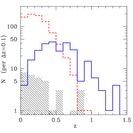
Figure 1: Redshift histograms of galaxy clusters with measured thermal SZE signals and redshifts from the literature. Solid line indicates 258 clusters detected in the ground-based surveys either by SPT spt09 ; spt10 ; spt11 ; spt13a or by ACT act10 ; act11 ; act13a , excluding overlaps, over a total of $\sim 3000$ deg². Dashed line shows 813 clusters detected by the Planck satellite over all sky planck_earlysz ; planck13a . For reference, hatched region marks 34 clusters with $>4\sigma$ SZE detections published as of 2002 (birkinshaw99 ; carlstrom02 and references therein) which consist mainly of X-ray luminous clusters.

The sensitivity of the SZE observations of individual clusters has also improved significantly, making it a useful tool for studying physics of intracluster plasma. In particular, the SZE data provide a direct measure of thermal pressure of electrons, which is highly complementary to X-ray observations. They allow us to study the distance-redshift relation (e.g., schmidt04 ; bonamente06 ), three-dimensional structures defilippis05 ; sereno12 , and dynamics kitayama04 ; korngut11 ; planck_coma of galaxy clusters. By means of the SZE, we are witnessing the high-mass end of structure formation in the Universe that in turn serves as a powerful probe of cosmology.

Theoretical foundations and earlier observations of the SZE are reviewed extensively by sz80b ; rephaeli95 ; birkinshaw99 ; carlstrom02 . In the present paper, we focus mainly on practical applications of the SZE that have become more feasible by recent observations, and discuss their cosmological and astrophysical implications. Unless explicitly stated otherwise and wherever necessary to assume specific values of cosmological parameters, we adopt a conventional $\Lambda$CDM model with the matter density parameter $\Omega_{\rm m}=0.3$, the dark energy density parameter $\Omega_{\Lambda}=0.7$, the baryon density parameter $\Omega_{\rm b}=0.045$, the Hubble constant $h_{70}=H_{0}/(70\mbox{\>km\>s${}^{-1}$Mpc${}^{-1}$})=1.0$, the dark energy equation of state parameter $w=-1.0$, the amplitude of density fluctuations $\sigma_{8}=0.8$, and the spectral index of primordial density fluctuations $n_{\rm s}=0.96$.

2 The Sunyaev-Zel’dovich Effect

When CMB photons pass through a cloud of free electrons with number density $n_{\rm e}$, they are subject to scattering with a probability characterized by the optical depth

$$\tau_{\rm e}=\int\sigma_{\rm T}n_{\rm e}dl\,\sim\,2\times 10^{-3}\left(\frac{n_{\rm e}}{10^{-3}\mbox{ cm}^{-3}}\right)\left(\frac{l}{\mbox{Mpc}}\right),$$ (1)

where $\sigma_{\rm T}$ is the Thomson cross section, $\int\cdots dl$ denotes the line-of-sight integral, and the quoted values are typical of galaxy clusters. It follows that a single scattering is in general a good approximation even in largest galaxy clusters. The Thomson limit applies in the rest frame of an electron as long as its velocity $v_{\rm e}$ relative to the CMB satisfies $\gamma_{\rm e}\equiv(1-v_{\rm e}^{2}/c^{2})^{-1/2}\ll m_{\rm e}c^{2}/(k_{\rm B}T_{\rm CMB})\sim 10^{9}/(1+z)$, where $m_{\rm e}$ is the electron mass, $c$ is the speed of light, $k_{\rm B}$ is the Boltzmann constant, and $T_{\rm CMB}$ is the CMB temperature. In the CMB rest frame, on the other hand, the net energy is transferred from the electron to the photons for $v_{\rm e}\gg\sqrt{k_{\rm B}T_{\rm CMB}/m_{\rm e}}\sim 10(1+z)^{1/2}$ km s^-1 and energies of the scattered photons increase by a factor of $\sim\gamma_{\rm e}^{2}$ on average. While such inverse Compton scattering takes place in a wide range of cosmic plasma, the term SZE is conventionally used for scattering of the CMB photons at GHz to THz frequencies by non-relativistic or mildly relativistic electrons. Its intensity is often expressed by a series of $v_{\rm e}/c$.

To the lowest order in $v_{\rm e}/c$, an apparent small change in $T_{\rm CMB}$ by the above scattering corresponds to the Doppler effect sz72 ; sz80a and called the kinematic SZE:

$$\frac{\Delta T_{\rm CMB}}{T_{\rm CMB}}=\int\sigma_{\rm T}n_{\rm e}\frac{v_{\parallel}}{c}dl\,\sim\,7\times 10^{-6}\left(\frac{n_{\rm e}}{10^{-3}\mbox{ cm}^{-3}}\right)\left(\frac{v_{\parallel}}{10^{3}~{}\mbox{km\>s${}^{-1}$}}\right)\left(\frac{l}{\mbox{Mpc}}\right),$$ (2)

where $v_{\parallel}$ is the line-of-sight component of $v_{\rm e}$ and is taken to have a positive value toward the observer. Equivalently, the CMB intensity spectrum is distorted by

$$\frac{\Delta I_{\nu}}{I_{\rm\nu,CMB}}=\frac{xe^{x}}{e^{x}-1}\int\sigma_{\rm T}n_{\rm e}\frac{v_{\parallel}}{c}dl,$$ (3)

where $I_{\rm\nu,CMB}=i_{0}x^{3}/(e^{x}-1)$, $i_{0}=2(k_{\rm B}T_{\rm CMB})^{3}/(h_{\rm P}c)^{2}$, $h_{\rm P}$ is the Planck constant, and $x$ is the dimensionless photon frequency $\nu$ defined by

$$x = \frac{h_{\rm P}\nu}{k_{\rm B}T_{\rm CMB}}=1.76\left(\frac{\nu}{100\mbox{~{}GHz}}\right)\left(\frac{T_{\rm CMB}}{2.726\mbox{~{}K}}\right)^{-1}.$$ (4)

Note that random velocities cancel out in equations (2) and (3) and the coherent motion with respect to the CMB is responsible for the kinematic SZE.

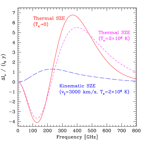
Figure 2: Spectra of the Sunyaev-Zel’dovich effect (SZE). Intensity differences from the CMB normalized by $i_{0}y$ are plotted for the non-relativistic thermal SZE (solid), the thermal SZE with the relativistic correction itoh04 for $T_{\rm e}=2\times 10^{8}$ K (short dashed), and the kinematic SZE with the relativistic correction nozawa06 for the bulk velocity $3000$ km s^-1 toward us and $T_{\rm e}=2\times 10^{8}$ K (long dashed). The ratio between the kinematic SZE and the thermal SZE is proportional to $v_{\parallel}/T_{\rm e}$ in the non-relativistic limit.

Isotropic random motions of Maxwellian electrons, on the other hand, give rise to the thermal SZE zs69 ; sz70 ; sz72 . For electrons with temperature $T_{\rm e}$ ($\gg T_{\rm CMB}$), the leading term of the spectral distortion is of order $(v_{\rm e}/c)^{2}\propto k_{\rm B}T_{\rm e}/(m_{\rm e}c^{2})$ and given by

$$\frac{\Delta T}{T_{\rm CMB}} = \left(x\coth\frac{x}{2}-4\right)\,y,$$ (5)

or equivalently,

$$\frac{\Delta I_{\nu}}{I_{\rm\nu,CMB}} = \frac{xe^{x}}{e^{x}-1}\left(x\coth\frac{x}{2}-4\right)\,y,$$ (6)

where $y$ is the Compton y-parameter:

$$y=\int\sigma_{\rm T}n_{\rm e}\frac{k_{\rm B}T_{\rm e}}{m_{\rm e}c^{2}}dl\,\sim\,4\times 10^{-5}\left(\frac{n_{\rm e}}{10^{-3}\mbox{ cm}^{-3}}\right)\left(\frac{T_{\rm e}}{10^{8}\mbox{ K}}\right)\left(\frac{l}{\mbox{Mpc}}\right),$$ (7)

which is essentially the dimensionless integrated electron pressure $P_{\rm e}=k_{\rm B}n_{\rm e}T_{\rm e}$.

Although the thermal SZE is of second order in $v_{\rm e}/c$, it dominates over the kinematic SZE typically by an order of magnitude for galaxy clusters because the thermal velocity of electrons $\sqrt{k_{\rm B}T_{\rm e}/m_{\rm e}}\sim 4\times 10^{4}(T_{\rm e}/10^{8}\mbox{K})^{1/2}$ km s^-1 is much larger than bulk velocities of $\lower 2.15277pt\hbox{$\;\buildrel<\over{\sim}\;$}10^{3}$ km s^-1. In the non-relativistic limit, spectral shapes of the kinematic SZE and the thermal SZE (eqs [3] and [6]) depend only on $x$. Corrections due to higher order terms are non-negligible once electrons become relativistic wright79 ; fabbri81 ; rephaeli95a ; challinor98 ; itoh98 ; sazonov98 ; nozawa98 . The spectral shape of the thermal SZE then starts to depend on $T_{\rm e}$ and that of the kinematic SZE on both $T_{\rm e}$ and the bulk velocity. In any case, observed amplitude and spectral shape of the SZE are both independent of $z$, because $\Delta T$ and $\Delta I_{\nu}$ are redshifted in exactly the same way as $T_{\rm CMB}$ and $I_{\rm\nu,CMB}$, respectively.

Figure 2 illustrates spectral shapes of the thermal SZE and the kinematic SZE for representative values of $T_{\rm e}$ and $v_{\parallel}$. The thermal SZE leads to a decrement at $\nu<218$ GHz ($x<3.83$) and an increment at higher frequencies. The relativistic correction shifts the null of the thermal SZE and modifies the spectral shape especially at high frequencies. The kinematic SZE, on the other hand, has its peak near the null of the thermal SZE. Multi-frequency measurements are necessary to separate the kinematic SZE from the thermal SZE and/or to determine $T_{\rm e}$ via the relativistic correction. Figure 3 further shows real images of a galaxy cluster, Abell 2256, taken by Planck planck_earlysz . Both decrement and increment signals of the thermal SZE are detected clearly at low and high frequencies, respectively. The data are also consistent with the null of the thermal SZE at 217 GHz, with no apparent signature of the kinematic SZE.

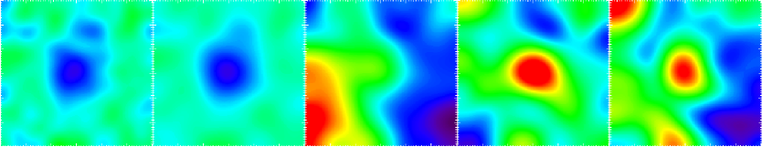
Figure 3: Cleaned images of Abell 2256 at $z=0.058$ observed by Planck at 100, 143, 217, 353, and 545 GHz from left to right over a size of $1^{\circ}\times 1^{\circ}$ (reproduced from planck_earlysz with permission, © ESO); $1^{\circ}=4.0\,h_{70}^{-1}$Mpc in the cluster rest frame. Blue, green, and red colors indicate negative, null, and positive intensities with respect to the CMB, respectively. The FWHMs of observing beams are $9.5^{\prime}$, $7.1^{\prime}$, $4.7^{\prime}$, $4.5^{\prime}$, and $4.7^{\prime}$ from left to right planck_hfi .

Small amounts of polarization are produced by inverse Compton scattering owing to anisotropies of the radiation field in the electron rest frame sz80a ; audit99 ; sazonov99 ; challinor00 ; itoh00 . Leading effects are due to i) the CMB quadrupole with the maximum polarization degree of $\sim 10^{-6}\tau_{e}$ toward the sky directions that are perpendicular to the quadrupole plane, ii) the transverse velocity $v_{\perp}$ of electrons on the sky with the polarization degrees of $\sim 0.1(v_{\perp}/c)^{2}\tau_{\rm e}$ and $\sim 0.01(v_{\perp}/c)\tau_{\rm e}^{2}$, and iii) thermal electrons with the polarization degree of $\sim 0.01(k_{\rm B}T_{\rm e}/m_{\rm e}c^{2})\tau_{\rm e}^{2}$; the prefactors are in the Rayleigh-Jeans limit and their frequency dependence as well as angular distribution can be found in sazonov99 . The effects proportional to $\tau_{\rm e}^{2}$ originate from multiple scatterings and are more sensitive to the spatial distribution of electrons. While all the effects are beyond the sensitivity of current detectors, they contain unique cosmological and astrophysical information. The first effect will provide a knowledge of the CMB quadrupole as seen by clusters including those at high redshifts, thereby reducing the cosmic variance uncertainty kamionkowski97 . The second effect, together with the kinematic SZE, will in principle offer a measure of the 3D velocity of the gas. The third effect will allow us to separate $T_{\rm e}$ and $\tau_{\rm e}$ in the thermal SZE.

Nonthermal electrons also upscatter the CMB photons. A number of galaxy clusters host diffuse synchrotron emission from relativistic electrons with $\gamma_{\rm e}\sim 10^{4}$ (see feretti12 for a review); while inverse Compton scattering by the same population of electrons should emerge in hard X-rays, their lower energy counterparts, if present, give rise to the nonthermal SZE. Predicted spectral distortions of the CMB, particularly at high frequencies, are sensitive to the underlying energy distribution of nonthermal electrons birkinshaw99 ; ensslin00 ; blasi00 ; colafrancesco03 . Major difficulties in actually observing them are the short life-time of suprathermal electrons as well as a large amount of contamination including the thermal SZE itself and dusty galaxies.

3 Evolution of the CMB Temperature

A fundamental prediction of the standard cosmology is that the CMB temperature evolves with redshift adiabatically as

$$T_{\rm CMB}(z)=T_{\rm CMB}(0)~{}(1+z),$$ (8)

where $T_{\rm CMB}(0)=2.7260\pm 0.0013$ K is the present-day CMB temperature measured by COBE-FIRAS fixsen09 . Any deviation from the above evolution would be a signature of a violation of conventional assumptions such as the local position invariance and the photon number conservation.

In fact, redshift-independence of the spectral shape of the SZE mentioned in Section 2 also relies on equation (8). This in turn makes it possible to use the observed SZE spectra to measure the CMB temperature fabbri78 ; rephaeli80 ; lamagna07 at an arbitrary $z$ and test the validity of equation (8). A great advantage of this method is that it uses only the spectral shape of the thermal SZE and does not rely, at least in principle, on details of underlying gas properties. In practice, appropriate gas distributions should be taken into account to correct for beam dilution effects at different observing frequencies. As long as the large-scale bulk motion is small (see Section 8), the kinematic SZE would primarily increase the dispersion of the measurement. The relativistic effects on the SZE can be suppressed by using clusters with relatively low electron temperatures; accurate temperature measurements of individual clusters will be necessary otherwise. Multi-frequency data will also be crucial for separating contamination by radio sources, CMB primary anisotropies, and dust emission.

A conventional approach of generalizing equation (8) is to adopt the form $T_{\rm CMB}(z)=T_{\rm CMB}(0)~{}(1+z)^{1-\beta_{\rm T}}$ lima00 and to determine the parameter $\beta_{\rm T}$ from the data. Recent SZE measurements for a sample of galaxy clusters give $\beta_{\rm T}=0.009\pm 0.017$ at $z<1$ using the Planck data at $100\sim 857$ GHz toward 813 clusters hurier13 and $\beta_{\rm T}=0.017^{+0.030}_{-0.028}$ at $z<1.35$ using the SPT data at 95 GHz and 150 GHz toward 158 clusters saro13 . Figure 4 shows that current measurements are consistent with the adiabatic prediction, while averaging over a large number of clusters is necessary owing to the variance inherent to individual clusters.

Figure 4: Measured redshift evolution of the CMB temperature as compared to the adiabatic prediction (dashed line). Red circles indicate the SZE measurements by stacking a sample of clusters detected by Planck hurier13 ; note that there are fewer clusters in each redshift bin at higher $z$ (see Fig. 1). Blue triangles show the SZE measurements for individual clusters luzzi09 . A cyan cross is the measurement using molecular absorption lines muller13 .

Another independent measure of the CMB temperature at $z>0$ comes from quasar absorption line spectra; if the relative population of the different energy levels of atoms or molecules are in radiative equilibrium with the CMB at that epoch, the excitation temperature of the species gives a measure of $T_{\rm CMB}(z)$ bahcall68 . Major sources of systematics are contributions of other heating sources, such as collisions and local radiation fields. Combining transition lines of various species are particularly useful for constraining the physical conditions of the absorbing gas; e.g., a comprehensive analysis of a molecular absorber at $z=0.89$ yields $T_{\rm CMB}=5.08\pm 0.10$ K muller13 in agreement with the adiabatic expectation of 5.15 K (Fig. 4). At $1.7<z<2.7$, the CMB temperatures derived from rotational excitation transitions of CO are also consistent with equation (8) noterdaeme11 .

In summary, the high significance measurements currently available are consistent with the adiabatic evolution of the CMB temperature and we assume it throughout this paper.

4 Distance Determinations

It has long been recognized that the thermal SZE and the X-ray emission from galaxy clusters provide a primary distance indicator that is entirely independent of the cosmic distance ladder cavaliere77 ; silk78 ; birkinshaw79 ; cavaliere79 . This method employs the fact that the SZE and the X-ray emission arise from the same thermal gas but depend on its density in a different manner (Sec. 4.1). Essentially the same method is readily applied to testing the distance duality relation uzan04 . Baryon fraction of galaxy clusters measured by X-ray and/or SZE observations can also be used to determine their distances sasaki96 ; pen97 (Sec. 4.2). Key assumptions in both methods are spherically symmetric and smooth distribution of the gas and impacts of possible violation of these assumptions are also discussed below.

4.1 Combination with X-ray data

Suppose that a galaxy cluster at redshift $z$ has radial profiles of electron density $n_{\rm e}(\phi)$ and temperature $T_{\rm e}(\phi)$ at the angular radius $\phi$ from its center, i.e., the physical radius in three dimensional space divided by the angular diameter distance $d_{\rm A}$ to the center. The X-ray surface brightness at the projected angle $\theta$ on the sky from the center is given by the line-of-sight integral:

$$I_{\rm X}(\theta)=\frac{2d^{3}_{\rm A}}{4\pi d^{2}_{\rm L}}\int_{\theta}^{\infty}n^{2}_{\rm e}(\phi)\Lambda_{\rm X}[T_{\rm e}(\phi),Z(\phi),z]\frac{\phi d\phi}{\sqrt{\phi^{2}-\theta^{2}}},$$ (9)

where $d_{\rm L}$ is the luminosity distance, $Z$ is the gas metallicity, and $\Lambda_{\rm X}$ is the X-ray cooling function including the k-correction, i.e., $n^{2}_{\rm e}\Lambda_{\rm X}$ stands for the energy radiated per unit time and unit volume in the rest frame of the cluster. In general, $\Lambda_{\rm X}$ depends only weakly on $T_{\rm e}$ (weaker than $T_{\rm e}^{1/2}$) within the limited energy band and a combination with X-ray spectral data allows one to measure $T_{\rm e}(\phi)$, $Z(\phi)$, and the shape of $n_{\rm e}(\phi)$ without the knowledge of $d_{\rm A}$ or $d_{\rm L}$ (see boehringer10 for a recent review), whereas the absolute value of $n_{\rm e}(\phi)$ does depend on the distances. Denoting $n_{\rm e}(\phi)=n_{\rm norm}f_{n}(\phi)$ to separate the normalization and the shape ($f_{n}(\phi)$ is dimensionless and normalized at some scale radius), one can rewrite equation (9) as

$$I_{\rm X}(\theta)=\frac{d^{3}_{\rm A}n^{2}_{\rm norm}}{d^{2}_{\rm L}}K_{\rm X}(\theta,z),$$ (10)

where observable quantities are

$$K_{\rm X}(\theta,z)\equiv\frac{1}{2\pi}\int_{\theta}^{\infty}f_{n}^{2}(\phi)\Lambda_{\rm X}[T_{\rm e}(\phi),Z(\phi),z]\frac{\phi d\phi}{\sqrt{\phi^{2}-\theta^{2}}}.$$ (11)

Similarly, the Compton y-parameter for the same cluster is given by

$$y(\theta)=d_{\rm A}n_{\rm norm}K_{\rm SZ}(\theta),$$ (12)

where

$$K_{\rm SZ}(\theta)\equiv\frac{2\sigma_{\rm T}k_{\rm B}}{m_{\rm e}c^{2}}\int_{\theta}^{\infty}f_{n}(\phi)T_{\rm e}(\phi)\frac{\phi d\phi}{\sqrt{\phi^{2}-\theta^{2}}}.$$ (13)

Eliminating $n_{\rm norm}$ from equations (10) and (12) gives

$$d_{\rm A}\eta^{2}=\frac{y^{2}(\theta)}{I_{\rm X}(\theta)(1+z)^{4}}\frac{K_{\rm X}(\theta,z)}{K^{2}_{\rm SZ}(\theta)},$$ (14)

where

$$\eta\equiv\frac{d_{\rm L}}{d_{\rm A}(1+z)^{2}}$$ (15)

is unity if the distance duality relation holds uzan04 . The right hand side of equation (14) consists of observables and gives a direct measure of $d_{\rm A}\eta^{2}$. For given $n_{\rm e}$, $T_{\rm e}$, and $Z$ as a function of the physical radius $d_{\rm A}\phi$, equations (9) and (12) indicate that $I_{\rm X}\propto\eta^{-2}(1+z)^{-4}$ and $y$ is independent of $z$, respectively.

Historically, equation (14) has been used widely to measure the Hubble constant assuming the distance duality relation ($\eta=1$) and the standard Friedmann-Lemaitre universe, in which case

$$d_{\rm A} = \frac{c}{H_{0}(1+z)}\left\{\begin{array}[]{ll}\frac{\sinh(\sqrt{\Omega_{\rm K}}~{}\chi)}{\sqrt{\Omega_{\rm K}}}&(\Omega_{\rm K}>0)\\ \chi&(\Omega_{\rm K}=0)\\ \frac{\sin(\sqrt{-\Omega_{\rm K}}~{}\chi)}{\sqrt{-\Omega_{\rm K}}}&(\Omega_{\rm K}<0)\end{array}\right.$$ (19)

where $\Omega_{\rm K}=1-\Omega_{\rm m}-\Omega_{\Lambda}$ and

$$\chi=\int_{0}^{z}\frac{dz^{\prime}}{\left[\Omega_{\rm m}(1+z^{\prime})^{3}+\Omega_{\rm K}(1+z^{\prime})^{2}+\Omega_{\Lambda}(1+z^{\prime})^{3(1+w)}\right]^{1/2}}\equiv\int_{0}^{z}\frac{dz^{\prime}}{E(z^{\prime})}.$$ (20)

Once the measurements attain sufficient accuracy, one will also be able to determine $\Omega_{\rm m}$, $\Omega_{\Lambda}$, and $w$ kobayashi96 . Early measurements assumed that the gas is isothermal ($T_{\rm e}(\phi)=$ constant) and tended to yield low values of $H_{0}$; e.g., a fit to the ensemble of 38 distance measurements compiled from the literature gave $H_{0}=60\pm 3$ km s^-1Mpc^-1 assuming $(\Omega_{\rm m},\Omega_{\Lambda},w)=(0.3,0.7,-1)$ carlstrom02 . More recent studies, that take account of the radial variation of $T_{\rm e}$ using spatially resolved X-ray spectroscopic observations by Chandra, report $H_{0}=69\pm 8$ km s^-1Mpc^-1 and $77^{+4+10}_{-3-8}$ km s^-1Mpc^-1 from 3 clusters at $0.09<z<0.45$ schmidt04 and 38 clusters at $0.14<z<0.89$ bonamente06 , respectively, for $(\Omega_{\rm m},\Omega_{\Lambda},w)=(0.3,0.7,-1)$. As noted by schmidt04 , direct temperature measurements were available out to about one-third of the virial radius for most clusters and the temperatures at larger radii were estimated assuming that the gas is in hydrostatic equilibrium with the gravitational potential inferred from numerical simulations nfw97 . Figure 5(a) compares the values of $d_{\rm A}$ measured by bonamente06 in such non-isothermal hydrostatic equilibrium model using the OVRO/BIMA SZE data and a range of theoretical predictions. As discussed later, a large scatter of the data is partly ascribed to asphericity of clusters and careful control of systematic errors will be crucial for improving the accuracy of the distance measurement.

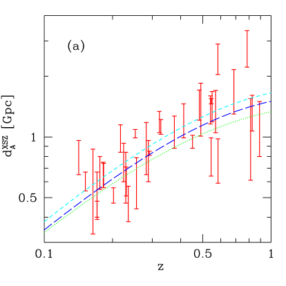
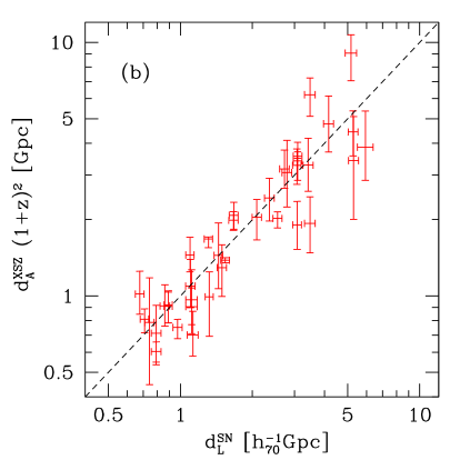
Figure 5: Left: (a) Angular diameter distances of 38 clusters measured by Chandra X-ray and OVRO/BIMA SZE data versus redshift bonamente06 . Lines indicate theoretical predictions for $(\Omega_{\Lambda},h_{70})=(0.7,1.0)$ (short dashed), $(0.7,1.1)$ (long dashed), and $(0,1.1)$ (dotted) assuming $\Omega_{\rm m}=0.3$, $w=-1$, and $\eta=1$. Right: (b) Same quantities multiplied by $(1+z)^{2}$ versus luminosity distances measured by the Union2.1 compilation of Type Ia supernova data suzuki12 . The values of $d_{\rm L}^{\rm SN}$ are the mean and its error of supernova distances whose redshifts match that of a galaxy cluster within $3\%$; there are on average 10 such supernovae per each cluster and an error due to the redshift differences is included in the error of $d_{\rm L}^{\rm SN}$. Dashed line marks the distance duality relation, $\eta=1$.

Alternatively, given the knowledge of cosmological parameters including $H_{0}$ from other measurements, e.g., CMB primary anisotropies and Cepheid variables, one can search for any departure from the distance duality relation using the same sets of data. Denoting the observable on the right hand side of equation (14) by $d_{\rm A}^{\rm XSZ}$, the quantity $\eta$ is written as

$$\eta=\sqrt{\frac{d_{\rm A}^{\rm XSZ}}{d_{\rm A}}},$$ (21)

or equivalently from equation (15),

$$\eta=\frac{d_{\rm A}^{\rm XSZ}}{d_{\rm L}}(1+z)^{2}.$$ (22)

One way of performing a consistency test is to use the predicted values of $d_{\rm A}$ from equation (19) in equation (21); $\eta$ should be unity over the range of redshifts considered if the distance duality relation holds and the correct cosmological model is used for $d_{\rm A}$ uzan04 ; bernardis06 . A more model-independent test is to use the measured values of $d_{\rm L}$, e.g., from Type Ia supernovae, in equation (22) nair11 ; cardone12 ; holanda12 . Figure 5(b) shows $d_{\rm A}^{\rm XSZ}(1+z)^{2}$ for 38 galaxy clusters from bonamente06 against $d_{\rm L}^{\rm SN}$ from the Union2.1 compilation of the Type Ia supernova data suzuki12 . For the latter, we extract from publicly available distance moduli of 580 supernovae the mean luminosity distance for those that fall within $|\Delta z|/z<0.03$ from each of 38 galaxy clusters; the range of $\Delta z$ is chosen so that its impact on the error of $d_{\rm L}^{\rm SN}$ is comparable to that from the distance modulus error and on average 10 supernovae are assigned for each cluster. Note that the supernovae only provide relative distance measurements and $h_{70}=1$ is assumed for determining the absolute magnitude in the Union2.1 compilation; i.e., $d_{\rm L}^{\rm SN}$ plotted in Figure 5(b) is proportional to $h_{70}^{-1}$. No significant deviation from $\eta=1$ has been detected in the current data out to $z\sim 0.8$. We will hence assume $\eta=1$ in the rest of this paper unless stated explicitly.

The distance determination by the SZE and X-ray technique is highly complementary to other astronomical methods and directly applicable to high redshifts. Controlling various systematic effects is crucial for improving its accuracy. First, a departure from spherical symmetry leads to overestimation of $d_{\rm A}$ (underestimation of $H_{0}$) if the cluster is elongated along the line-of-sight and vice versa; as described in Section 6, this property can in turn be used for studying the gas distribution. While asphericity primarily enhances the scatter of measurements, there may also be a systematic bias owing to the fact that such elongated clusters are brighter and easier to observe; it has been pointed out that strongly elongated clusters are preferentially aligned along the line-of-sight in a sample of 25 X-ray selected clusters with existing SZE data defilippis05 . Measurements using a homogeneous sample in both X-rays and SZE will be crucial for eliminating this bias. Second, clumpiness in the gas density will reduce $y^{2}/I_{\rm X}\sim\langle n_{\rm e}\rangle^{2}/\langle n_{\rm e}^{2}\rangle$ in equation (14) and bias the value of $d_{\rm A}$ low, possibly by $10-20\%$ inagaki95 . On the other hand, inhomogeneities of the gas temperature give rise to overestimation of $d_{\rm A}$ and may surpass the bias by the density clumpiness kawahara08 . Third, unresolved point sources in the SZE decrement/increment data will reduce/enhance the estimated value of $d_{\rm A}$. Finally, calibration uncertainties of absolute intensities and the temperature in X-ray and SZE observations are likely to be responsible for additional $10-20\%$ errors (e.g., reese10 ).

4.2 Gas mass fraction of galaxy clusters

Largest clusters of galaxies have grown out of density fluctuations spread over a comoving scale of $>10$ Mpc and are expected to be fair samples of the matter content of the Universe. Their baryonic-to-total mass ratio should therefore provide a measure of $\Omega_{\rm b}/\Omega_{\rm m}$ white93 ; if a part of baryonic mass in clusters is observed, a robust lower bound to $\Omega_{\rm b}/\Omega_{\rm m}$ can still be obtained. Furthermore, the fact that the baryon fraction should be constant with redshifts can be used to measure the distances independently of the absolute value of $\Omega_{\rm b}/\Omega_{\rm m}$ sasaki96 ; pen97 as described below.

Baryons in clusters are dominated by hot thermal plasma observed with X-rays and the SZE. The intracluster plasma is almost fully ionized and close to the primordial composition of hydrogen and helium plus a small fraction ($<1\%$ in weight) of heavier elements. The gas mass can therefore be measured by integrating $n_{\rm e}$ over the volume. From equations (9) and (12), $M_{\rm gas}\propto\int n_{\rm e}dV\propto n_{\rm norm}d^{3}_{\rm A}$ gives

$$M_{\rm gas,X}\propto d_{\rm L}d_{\rm A}^{3/2},$$ (23)

and

$$M_{\rm gas,SZ}\propto d_{\rm A}^{2},$$ (24)

for X-rays and the SZE, respectively.

Observations of the intracluster gas further provide a measure of the total mass enclosed within a physical radius $r=d_{\rm A}\phi$ on the assumption that the gas is in hydrostatic equilibrium with the gravitational potential as

$$M(<r)=-\frac{r}{G}\frac{k_{\rm B}T_{\rm e}(r)}{\mu m_{\rm p}}\left[\frac{d\ln n_{\rm e}(r)}{d\ln r}+\frac{d\ln T_{\rm e}(r)}{d\ln r}\right],$$ (25)

where $\mu$ is the mean molecular weight and $m_{\rm p}$ is the proton mass. Equation (25) does not depend on the absolute value of $n_{\rm e}$ (or that of pressure $P_{\rm e}\propto n_{\rm e}T_{\rm e}$) and scales linearly with the distance as $M\propto d_{\rm A}$. The total mass can also be estimated using galaxy velocity dispersions or gravitational lensing with the similar scaling with the distance to the cluster (strictly speaking, lensing mass depends on the relative positions of the source and the cluster which introduce an additional weak cosmological dependence). In practice, the mass can be measured within a finite radius often expressed in terms of a scaled radius $R_{\Delta}$, defined as the radius within which the average matter density is $\Delta$ times the critical density of the Universe; e.g., $R_{2500}$ and $R_{500}$ correspond to about 20% and 50%, respectively, of the virial radius ($\simeq R_{100}$) at $z=0$ for the mass profile inferred from numerical simulations nfw97 . Likewise, $M_{\Delta}$ denotes the total mass enclosed within $R_{\Delta}$ and they are related by

$$R_{\Delta}=1.5\mbox{~{}Mpc}\left(\frac{M_{\Delta}}{10^{15}M_{\odot}}\right)^{1/3}\left(\frac{\Delta}{500}\right)^{-1/3}h_{70}^{-2/3}E(z)^{-2/3},$$ (26)

where $E(z)$ is defined in equation (20).

Taken together, the gas mass fraction $f_{\rm gas}=M_{\rm gas}/M$ in clusters depends on the distance as

$$f_{\rm gas,X}\propto d_{\rm L}d_{\rm A}^{1/2}\propto d_{\rm A}^{3/2}(1+z)^{2}\eta,$$ (27)

and

$$f_{\rm gas,SZ}\propto d_{\rm A},$$ (28)

for gas masses measured with X-rays and the SZE, respectively. Equation (27) implies that one can also test the distance duality relation using $f_{\rm gas,X}$ if it is intrinsically constant over the range of redshifts observed goncalves12 . While $f_{\rm gas,SZ}$ depends on $d_{\rm A}$ more weakly than $f_{\rm gas,X}$, it has an advantage of being less sensitive to clumpiness of the gas. As expected, equating the two quantities, $f_{\rm gas,X}=f_{\rm gas,SZ}$, recovers essentially the same measure of the distance as equation (14). Obviously, possible evolution of the other baryon components such as stars and the gas depleted from the clusters is the major source of systematic errors and needs be properly taken into account.

For the same set of 38 clusters as the one used for the $H_{0}$ measurement in bonamente06 , the inferred gas mass fraction is consistent with a constant value of $f_{\rm gas,SZ}\simeq 0.12\,h_{70}^{-1}$ within $R_{\rm 2500}$, albeit with a large scatter, over $0.14<z<0.89$ for $(\Omega_{\rm m},\Omega_{\Lambda},w)=(0.3,0.7,-1)$ laroque06 . This is in agreement with independent SZE measurements by VSA lancaster05 and AMiBA umetsu09 as well as measured values of $f_{\rm gas,X}$ allen08 ; vikhlinin09a ; ettori09 ; it corresponds to $\sim 80\%$ of the cosmic mean value $\Omega_{\rm b}/\Omega_{\rm m}$ from the Planck 2013 results planck_cosm . Observed $f_{\rm gas,X}$ of nearby clusters tends to increase with the radius from the cluster center vikhlinin06 ; zhang10 ; simionescu11 ; eckert13b and it may partly be due to clumpiness and substructures. It will hence be meaningful to improve the sensitivities of the $f_{\rm gas,SZ}$ measurements particularly at large radii ($>R_{\rm 500}$). Since the SZE directly measures the gas mass projected on the sky times the mass-weighted temperature (eq. [29]), it can also be combined with the projected total mass from weak lensing to yield cylindrical $f_{\rm gas,SZ}$ without an assumption of spherical symmetry holder00 .

5 Source Counts

The ability to find a galaxy cluster in SZE surveys is primarily limited by its flux, which is proportional to equation (12) integrated over the sky,

$$S_{\rm SZ}\propto\int y(\theta)d^{2}\theta\propto\frac{1}{d^{2}_{\rm A}}\int n_{\rm e}T_{\rm e}dV\propto\frac{M_{\rm gas}\langle T_{\rm e}\rangle}{d^{2}_{\rm A}},$$ (29)

where $\langle\cdots\rangle$ denotes the mass-weighted average. Since $d_{\rm A}$ depends on $z$ only weakly at $z>0.5$ and $T_{\rm e}$ correlates with mass, flux-limited SZE surveys become nearly mass-limited at high redshifts. The X-ray flux, on the other hand, is given from equation (9) as

$$S_{\rm X}=\int I_{\rm X}(\theta)d^{2}\theta\propto\frac{1}{d^{2}_{\rm L}}\int n^{2}_{\rm e}\Lambda_{\rm X}(T_{\rm e},Z,z)dV.$$ (30)

While a rapid increase of $d^{2}_{\rm L}$ with $z$ is partly canceled by the evolution of $n_{\rm e}$, finding low-mass clusters becomes more challenging at higher $z$ in flux-limited X-ray surveys. Typical radius of a galaxy cluster $\sim$ Mpc (eq. [26]) corresponds to $\sim 2^{\prime}$ at $z=1$ and angular resolution better than this scale is also necessary to identify distant clusters. A rapid decrease in the number of galaxy clusters detected by Planck with redshift shown in Figure 1 is likely due to its moderate spatial resolution of $\lower 2.15277pt\hbox{$\;\buildrel>\over{\sim}\;$}5^{\prime}$ planck_hfi , whereas SPT and ACT are designed for finding clusters up to high $z$ with beam FWHMs at 150 GHz of $1.2^{\prime}$ spt09 and $1.4^{\prime}$ act10 , respectively. On the other hand, Planck covers a wider frequency range up to $>300$ GHz and is more suitable for observing nearby clusters including their SZE increment signals (Fig. 3).

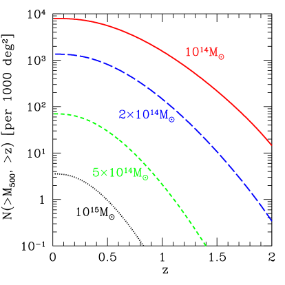
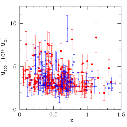
Figure 6: Left: Predicted numbers of galaxy clusters per 1000 deg² above given redshift $z$ and mass $M_{500}$. The numbers are plotted for $M_{500}=10^{14}M_{\odot}$ (solid), $2\times 10^{14}M_{\odot}$ (long dashed), $5\times 10^{14}M_{\odot}$ (short dashed), and $10^{15}M_{\odot}$ (dotted), using the mass function of tinker08 and assuming the conventional $\Lambda$CDM universe. Right: Estimated masses versus redshifts of galaxy clusters detected in the surveys by SPT in 720 deg² (red circles, spt13a ) and ACT in 504 deg² (blue crosses, act13a ). The plotted are 158 and 68 clusters confirmed by optical/infrared imaging and include 117 and 19 new discoveries, respectively.

The expected number of sources per unit solid angle above the flux $S$ between redshifts $z_{\rm min}$ and $z_{\rm max}$ can be written as (e.g., kss98 )

$$N(>S,z_{\rm min},z_{\rm max})=\int_{z_{\rm min}}^{z_{\rm max}}dz\frac{dV}{d\Omega dz}\left.\int_{S}^{\infty}dS^{\prime}\frac{dn(M,z)}{dM}\frac{dM}{dS^{\prime}}\right|_{M=M(S^{\prime},z)},$$ (31)

where $dn(M,z)$ is the comoving number density of galaxy clusters of mass $M\sim M+dM$ corresponding to flux $S^{\prime}\sim S^{\prime}+dS^{\prime}$ at $z$ and

$$\frac{dV}{d\Omega dz}=\frac{c}{H_{0}}\frac{(1+z)^{2}d_{\rm A}^{2}(z)}{E(z)}$$ (32)

is the comoving volume element per unit solid angle and unit redshift. For given initial distribution and evolution thereafter of primordial density fluctuations, the mass function $dn(M,z)/dM$ can be computed using either analytic prescriptions (e.g., ps74 ; sheth99 ) or state-of-the-art numerical simulations (e.g., jenkins01 ; tinker08 ), on the assumption that every virialized dark matter halo above some threshold mass becomes a galaxy cluster. The relation between the observed flux and the mass is often estimated by means of empirical scaling relations calibrated by local observations (e.g., vikhlinin09a ; arnaud10 ). Comparisons with observed numbers of clusters then give a measure of cosmological parameters through both the growth of density fluctuations and the geometry of the Universe.

Figure 6 illustrates the number counts of galaxy clusters predicted in the conventional $\Lambda$CDM model as well as estimated masses versus redshifts of clusters detected in the SZE surveys. Current surveys by SPT and ACT have been finding clusters down to $M_{500}\simeq 2\times 10^{14}M_{\odot}$ up to $z\sim 1.5$ over the fields of nearly 1000 square degrees spt13a ; act13a . It should be noted that completeness of the samples degrades toward low mass and the estimated masses may be biased particularly at higher $z$ since they are based on empirical relations extrapolated from low $z$. Within such uncertainties, the detected numbers are consistent with the predictions and it is likely that one will start to find clusters at $z>2$ by reaching deeper fluxes corresponding to $M_{500}<10^{14}M_{\odot}$.

The predicted numbers of clusters are the most sensitive to underlying values of $\Omega_{\rm m}$ and $\sigma_{8}$. Recent results using a sample of 189 clusters from the Planck SZE catalog indicate $\sigma_{8}(\Omega_{\rm m}/0.27)^{0.3}=0.764\pm 0.025$ planck_counts . This is in agreement with other measurements in the local Universe using SZE cluster counts by SPT benson13 ; spt13a and ACT act13a , X-ray cluster counts vikhlinin09b and cosmic shear kilbinger13 , whereas it tends to be smaller than that inferred from CMB primary anisotropies measured by Planck planck_cosm . The origin of this tension is still not entirely clear but may be ascribed to incomplete instrumental calibration, underestimating true masses of clusters, missing a fraction of massive clusters, suppression of density fluctuations at small scales by, e.g., massive neutrinos, or any combination thereof.

Since clusters of galaxies comprise the largest virialized structures in the Universe, the evolution of their numbers up to high $z$ provides a sensitive probe of the growth of cosmic structures, which is highly complementary to purely geometrical methods such as Type Ia supernovae and Baryon Acoustic Oscillations. It can be used to explore the nature of dark energy within a framework of standard cosmology (e.g., vikhlinin09b ; mantz10 ) as well as to search for any departure from the standard framework itself. For instance, the linear growth rate of density fluctuations $D$ can be generalized as wang98 ; linder05

$$\frac{d\ln D}{d\ln a}=\Omega_{\rm m}(a)^{\gamma_{\rm g}},$$ (33)

where $a=1/(1+z)$ is the cosmic scale factor, $\Omega_{\rm m}(a)=\Omega_{\rm m}a^{-3}E^{-2}(a)$, and the index $\gamma_{\rm g}$ takes nearly a constant value $\simeq 0.55$ if general relativity holds. This will allow one to constrain the growth of structures and the geometry of the Universe separately from the data. Current X-ray cluster data are fully consistent with general relativity rapetti13 and the analysis can be refined further by including higher $z$ clusters such as those observed by the SZE.

It should be noted that the applicability of cluster counts as a cosmological probe relies critically on the accuracy of mass determination. This is a challenging issue particularly at $z>1$, where spatially resolved X-ray spectroscopy or weak lensing becomes increasingly difficult; even if empirical scaling relations are to be used, they must be calibrated by some independent means. To this end, SZE imaging observations will further offer a useful measure of the mass as described in Section 6.

6 Structure of Intracluster Plasma

The accuracy of cosmological studies using the SZE is largely limited by our understanding of astrophysics of galaxy clusters. Historically, internal structure of the intracluster plasma has been studied extensively by X-ray observations. As mentioned in Section 4.1, radial profiles of $n_{\rm e}$ and $T_{\rm e}$ have been measured by X-ray surface brightness and spectra for a large number of clusters. Modeling the SZE brightness using equation (12) or the total mass using equation (25) also relied on these measurements for decades. Detailed X-ray spectroscopic observations, however, become progressively difficult for distant clusters or toward the outskirts of even nearby clusters (see reiprich13 for a review), owing to low photon counts and background contamination. Recent developments of high sensitivity and high resolution SZE observations have opened up new possibilities as described below.

Figure 7: Data points show radial pressure profiles from the Bolocam SZE data for 45 clusters at $0.15<z<0.89$ assuming $(\Omega_{\rm m},\Omega_{\Lambda},w,h_{70})=(0.3,0.7,-1,1)$ (reproduced from sayers13a with permission, © AAS); full sample (left panel), a subsample of disturbed clusters (middle panel), and a subsample of cool-core (apparently relaxed) clusters (right panel). Also shown are the fits by a parametric model of equation (34) for this sample (shaded regions indicating the 68.3% confidence region), a sample of 33 X-ray clusters at $z<0.2$ by Arnaud et al. arnaud10 (solid line), and a sample of 62 Planck-selected clusters at $z\sim 0.15$ planck_intv (dashed line).

First of all, a spatially resolved thermal SZE image alone yields the radial profile of electron pressure under the assumption of spherical symmetry. Figure 7 shows deprojected pressure profiles from the SZE data taken by Bolocam sayers13a . Radially averaged pressure at $0.2R_{500}<r<R_{500}$ is rather insensitive to dynamical status of clusters and is well represented by the following functional form nagai07 ; arnaud10 ,

$$\frac{P_{\rm e}}{P_{500}}=\frac{P_{0}}{(C_{500}X)^{\alpha_{3}}[1+(C_{500}X)^{\alpha_{1}}]^{(\alpha_{2}-\alpha_{3})/\alpha_{1}}},$$ (34)

where $X=r/R_{500}$, $(P_{0},C_{500},\alpha_{1},\alpha_{2},\alpha_{3})$ are fitting parameters, and $P_{500}$ is the scaled pressure defined by

$$P_{500}=1.65{\rm~{}eV~{}cm}^{-3}\left(\frac{M_{500}}{3\times 10^{14}h_{70}^{-1}M_{\odot}}\right)^{\beta_{\rm P}}h_{70}^{2}E(z)^{8/3}.$$ (35)

Apart from the fact that slightly different values of $\beta_{\rm P}$ are used in the literature (e.g., 0.67 in sayers13a and 0.79 in arnaud10 ; planck_intv ), the above pressure profile accounts for the X-ray data of nearby clusters arnaud10 as well as the SZE data by SPT plagge10 , CARMA bonamente12 , and Planck planck_intv . Discrepant results, on the other hand, are reported on three individual clusters between AMI and Planck planck_ami , suggesting a presence of yet unaccounted for systematic effects. Dispersion of the reconstructed pressure profile provides a key consistency check of the applicability of the mass estimation assuming hydrostatic equilibrium (eq. [25]) or any empirical scaling relations based on it.

Second, one can combine the SZE image with the X-ray surface brightness map to recover radial profiles of $n_{\rm e}$ and $T_{\rm e}$ separately without X-ray spectroscopic data. This is done essentially by inverting equations (9) and (12) using the Abel transform silk78 ; yoshikawa99 ,

$$n_{\rm e}(\phi)^{2}\Lambda_{\rm X}[T_{\rm e}(\phi),Z(\phi),z] = \frac{4d^{2}_{\rm L}}{d^{3}_{\rm A}}\int_{\phi}^{\infty}\left[-\frac{dI_{\rm X}(\theta)}{d\theta}\right]\frac{d\theta}{\sqrt{\theta^{2}-\phi^{2}}},$$ (36)

$$n_{\rm e}(\phi)T_{\rm e}(\phi) = \frac{m_{\rm e}c^{2}}{\pi k_{\rm B}\sigma_{\rm T}d_{\rm A}}\int_{\phi}^{\infty}\left[-\frac{dy(\theta)}{d\theta}\right]\frac{d\theta}{\sqrt{\theta^{2}-\phi^{2}}},$$ (37)

and separating $n_{\rm e}(\phi)$ and $T_{\rm e}(\phi)$; $\Lambda_{\rm X}$ depends only weakly on $Z$ for $T_{\rm e}\lower 2.15277pt\hbox{$\;\buildrel>\over{\sim}\;$}2\times 10^{7}$ K. Note that an assumption on underlying cosmology is necessary only to determine an absolute value of $n_{\rm e}$ or $T_{\rm e}$ and not to reconstruct the shape of their profiles. Practical applications of the above inversion have become possible during the last decade kitayama04 ; yuan08 ; nord09 ; basu10 ; eckert13 . A great advantage of this method is that it is applicable to X-ray faint regions as long as imaging data are available; its feasibility has been tested against existing X-ray spectroscopic measurements as illustrated in Figure 8. Further invoking an assumption of hydrostatic equilibrium (eq. [25]), it offers a unique measure of the gravitational mass at high redshifts and large radii.

Figure 8: Deprojected electron density (left panel) and temperature (right panel) of Abell 2204 at $z=0.152$ from a joint analysis of the APEX-SZ SZE image and the XMM-Newton X-ray brightness (reproduced from basu10 with permission, © ESO). For reference, the dashed line and red diamonds show the results of X-ray analysis using the spectral data zhang08 .

Finally, if an independent measure of $T_{\rm e}$ is also available through X-ray spectroscopy, one can relax the assumption of spherical symmetry and explore intrinsic shapes of galaxy clusters for a given cosmological model. This is in fact an alternative to the distance determination described in Section 4.1; a cluster elongated by some fraction over the line-of-sight will enhance the value of $d_{\rm A}$ in equation (14) by the same fraction. Observed X-ray images of galaxy clusters have projected axis ratios with a mean $\simeq 0.8$ and a dispersion $\simeq 0.1$ defilippis05 ; kawahara10 , and the SZE data will further add line-of-sight information. For example, X-ray and multi-frequency SZE data of Abell 1689 can be explained well by a mildly triaxial cluster with a minor to major axis ratio of $0.7\pm 0.15$, preferentially elongated along the line of sight sereno12 . One can further explore the 3D orientation of the dark matter halo by combining weak lensing data and assuming, for instance, that the gas is in hydrostatic equilibrium morandi11 or it shares the same axis directions with the dark matter sereno13 . Note that the SZE brightness of an individual cluster at a single frequency can be biased by the kinematic SZE; Figure 9 illustrates that a combination of multi-frequency data, particularly of both decrement ($\nu<218$ GHz) and increment ($\nu>218$ GHz) of the SZE, is useful for breaking the degeneracy between the line-of-sight elongation and the peculiar velocity.

Figure 9: Limits on the line-of-sight elongation factor and the peculiar velocity of RX J1347.5–1145 from multi-frequency SZE data (reproduced from kitayama04 with permission, © ASJ); the cluster is modeled by a spheroid elongated along the line-of-sight. The thick solid contours indicate the 68.3, 95.4, and 99.7% confidence regions from a joint fit to the data at three frequencies. The other contours show the 68.3% confidence region from each of the 350 GHz (thick dotted), 150 GHz (thin solid), and 21 GHz (thin dotted) data separately. The 150 GHz image of this cluster is shown in Fig. 10 and the disturbed substructure is excluded in the analysis shown here.

7 Dynamics of Galaxy Clusters

Clusters of galaxies often display signatures of violent mergers, which comprise the most energetic phenomena in the Universe with the total kinematic energy $\sim 10^{64}$ ergs and mark directly the sites of cosmic structure formation. Associations with synchrotron emission from nonthermal electrons indicate that a certain degree of particle acceleration is also induced during cluster mergers, although the precise mechanism is still unknown. While X-ray and low-frequency ($\;\buildrel<\over{\sim}\;$GHz) radio observations have been widely used to find such merger shocks at low redshifts (see markevitch07 ; feretti12 for reviews), the SZE provides a promising and complementary diagnostics up to high redshifts. Since the thermal SZE and the kinematic SZE are proportional to thermal pressure and the bulk velocity, respectively, they serve as direct probes of shock fronts (i.e., pressure gaps) and gas dynamics. In addition, SZE images with a spatial resolution of $\sim 10^{\prime\prime}$ komatsu01 ; mason10 or better will continue to play a unique role in resolving the shock-heated gas with $k_{\rm B}T_{\rm e}\gg 10$ keV, given that spatial resolutions of current and near future hard X-ray ($E>10$ keV) instruments are limited to $>45^{\prime\prime}$. By measuring a gap across the shock of either density, temperature, or pressure, one can infer the Mach number $\mathcal{M}$ (i.e., gas velocity normalized by its sound speed in the rest frame of the shock front) from Rankine-Hugoniot relations:

$$\frac{n_{\rm 2}}{n_{\rm 1}}=\frac{v_{1}}{v_{2}}=\frac{4\mathcal{M}_{1}^{2}}{\mathcal{M}_{1}^{2}+3},~{}~{}~{}~{}\frac{T_{\rm 2}}{T_{\rm 1}}=\frac{(5\mathcal{M}_{1}^{2}-1)(\mathcal{M}_{1}^{2}+3)}{16\mathcal{M}_{1}^{2}},$$ (38)

where the subscripts 1 and 2 denote preshock and postshock quantities respectively, and an adiabatic index of $\gamma=5/3$ has been used. The product of these equations readily yield the pressure ratio.

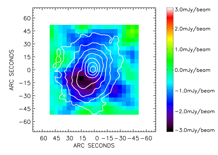
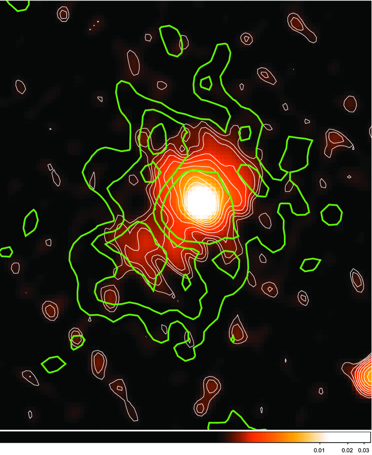
Figure 10: Observed images of RX J1347.5-1145 at $z=0.451$; $1^{\prime\prime}=5.8\,h_{70}^{-1}$ kpc in the cluster rest frame. Left: NOBA 150 GHz SZE map with $13^{\prime\prime}$ beam FWHM smoothed by a $15^{\prime\prime}$ Gaussian filter for display komatsu01 , overlaid with Chandra 0.5–7keV X-ray brightness contours (reproduced from kitayama04 with permission, © ASJ). Right: GMRT 614 MHz synchrotron intensity map and contours (white), overlaid with MUSTANG 90 GHz SZE contours with $9^{\prime\prime}$ beam FWHM mason10 (reproduced from ferrari11 with permission, © ESO). There is a radio point source at the cluster center in both images, which reduces the thermal SZE decrements and enhances the synchrotron intensities.

A prototype of intensive SZE studies on a merging cluster is given by those on RX J1347.5-1145 at $z=0.451$, the brightest cluster known to date in the SZE. This cluster was originally thought to be highly relaxed, based on smooth morphology of the soft X-ray ($E<2$ keV) image by ROSAT schindler97 . The SZE observation by NOBA with $13^{\prime\prime}$ beam komatsu01 , however, revealed that it has a prominent substructure at $\sim 20^{\prime\prime}$ southeast of the cluster center as shown in Figure 10. This finding has been confirmed subsequently with Chandra 0.5–7 keV data allen02 as well as more recent high sensitivity SZE images by MUSTANG with $9^{\prime\prime}$ beam mason10 ; korngut11 and by CARMA with the smallest synthesized beam of $11^{\prime\prime}\times 17^{\prime\prime}$ plagge13 . Independent SZE measurements of this cluster have also been published using SCUBA komatsu99 ; kitayama04 ; zemcov07 , Diabolo pointecouteau99 ; pointecouteau01 , OVRO/BIMA reese02 ; carlstrom02 , SuZIE benson04 , Bolocam and Z-Spec zemcov12 . The inferred temperature of the substructure is $k_{\rm B}T_{\rm e}\simeq 25$ keV, which is about a factor of $2$ higher than the mean temperature of this cluster $k_{\rm B}T_{\rm e}\simeq 13$ keV kitayama04 ; ota08 ; this is in accord with the fact that the substructure is more obvious in the SZE than soft X-rays. It follows that the cluster is probably undergoing a major merger; applying equation (38) to the above mentioned temperatures gives the Mach number of $\mathcal{M}_{1}\simeq 1.9$ and the corresponding pre-shock velocity of $v_{1}\simeq 3500$ km s^-1. Figure 10 further illustrates that diffuse synchrotron emission from non-thermal electrons is spatially associated with the hot substructure gitti07 ; ferrari11 .

Merger shocks have also been detected using the SZE for other clusters including MACS0744.8+3927 at $z=0.69$ with an inferred value of the Mach number $\mathcal{M}_{1}\simeq 1.2$ korngut11 and Coma at $z=0.023$ with $\mathcal{M}_{1}\simeq 2.0$ planck_coma . The fraction of merging clusters is likely to increase with redshifts as the growth of density fluctuations becomes faster prior to the onset of cosmic acceleration. It is likely that the SZE surveys will continue to find a number of new merging clusters as demonstrated by a discovery of ACT-CL J0102–4915 at $z=0.87$ menanteau12 .

The kinematic SZE also gives a direct probe of the gas velocity. The measurement is in general challenging for individual clusters (e.g., zemcov12 ), but becomes feasible if a major merger is taking place along the line-of-sight and high quality SZE data are available at multi-frequencies. In fact, the line-of-sight velocity of $v_{\parallel}=-3450\pm 900$ km s^-1 has been reported for a subcluster of MACS J0717.5+3745 at $z=0.55$ using 140 GHz and 268 GHz Bolocam data sayers13b . Such measurements are highly complementary to future high-dispersion X-ray spectroscopic observations using micro-calorimeters on board ASTRO-H and ATHENA.

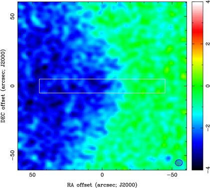
Figure 11: Simulations of the shock front in 1E 0657-558 (Bullet cluster) at $z=0.296$ (reproduced from yamada12 with permission, © ASJ); $1^{\prime\prime}=4.4\,h_{70}^{-1}$kpc in the cluster rest frame. Left: Expected SZE image by ALMA at 90GHz including various noise components. The color units are in $\mu$Jy/arcsec². Right: Error bars are the expected SZE intensities in the region marked by a white box in the left panel, whereas thick dashed line is the input hydrodynamical model before adding noise. Vertical thin lines indicate the positions of the shock front (thin dashed) and the contact discontinuity (thin dotted), respectively.

In near future, ALMA will be capable of imaging the SZE in bright compact clusters with the spatial resolution of $5^{\prime\prime}$ or better yamada12 . Figure 11 demonstrates that ALMA is indeed a powerful tool for resolving the shock front, characterized by temperature and pressure jumps. Shocks in galaxy clusters are in general hard to find in X-rays because they often appear at outskirts and are also hidden by a sharp radial gradient of $n_{\rm e}^{2}$; density peaks behind the contact discontinuity are much easier to be seen in X-rays as cold fronts (e.g., markevitch07 ). The SZE and X-rays are thus complementary in probing the detailed shock structure and the former is particularly useful for detecting hot rarefied gas. The spatial resolution of $5^{\prime\prime}$ is indeed crucial for resolving the physical scale comparable to the Coulomb mean free path ($\sim 20$ kpc) of electrons and protons in distant clusters. ALMA will also be able to simultaneously identify and remove point sources that often contaminate the diffuse SZE.

8 Unresolved Structures of the Universe

Recent developments of data sets over large sky areas have opened several possibilities of probing yet unresolved structures of the Universe by means of the SZE.

First, it has long been suggested that the integrated thermal SZE signal, including low-mass clusters and groups of galaxies, contributes to the CMB temperature anisotropies at sub-degree angular scales ck88 ; ss88 ; markevitch92 ; makino93 ; bartlett94 . The angular power spectrum of the Compton y-parameter can be written as $C^{\rm yy}_{l}=C_{l}^{\rm yy(P)}+C_{l}^{\rm yy(C)}$, where $C_{l}^{\rm yy(P)}$ is the contribution from the Poisson noise and $C_{l}^{\rm yy(C)}$ is from correlation among the sources. Employing the Limber’s approximation limber53 , one can write down these terms as kk99

$$C_{l}^{\rm yy(P)} = \int_{z_{\rm min}}^{\infty}dz\frac{dV}{d\Omega dz}\int_{M_{\rm min}}^{M_{\rm max}}dM\frac{dn(M,z)}{dM}\left|\tilde{y}_{l}(M,z)\right|^{2},$$ (39)

$$C_{l}^{\rm yy(C)} = \int_{z_{\rm min}}^{\infty}dz\frac{dV}{d\Omega dz}P_{\rm m}\left(k,z\right)\left[\int_{M_{\rm min}}^{M_{\rm max}}dM\frac{dn(M,z)}{dM}b(M,z)\tilde{y}_{l}(M,z)\right]^{2},$$ (40)

where $P_{\rm m}(k,z)$ is the 3D matter power spectrum, $k=l/(1+z)/d_{\rm A}$ is the comoving wave number, $b(M,z)$ is the linear bias factor of dark matter halos mw96 ; sheth99 . The 2D angular Fourier transform of the Compton y-parameter is given by ks02

$$\tilde{y}_{l}(M,z)=4\pi d_{\rm A}(z)\frac{\sigma_{\rm T}}{m_{\rm e}c^{2}}\int_{0}^{\infty}P_{\rm e}(\phi,M,z)\frac{\sin(l\phi)}{l\phi}\phi^{2}d\phi,$$ (41)

where $P_{\rm e}(\phi,M,z)$ is electron pressure at an angular radius $\phi$ from the center of a cluster of mass $M$ at redshift $z$. Figure 12 shows an updated version of predictions by kk99 in the conventional $\Lambda$CDM model using the mass function by tinker08 and the pressure profile of equations (34) and (35) with the parameters given in arnaud10 . The Poisson component is dominated by massive nearby clusters, which will be identified individually. Once they are removed, the remaining power is governed by low mass clusters at higher redshifts, with an increasing contribution from the correlation component. The power at $l\lower 2.15277pt\hbox{$\;\buildrel<\over{\sim}\;$}1000$ will also provide a sensitive measure of $\sigma_{8}$, whereas it depends on details of underlying pressure profile at higher multipoles (e.g., efstathiou12 ).

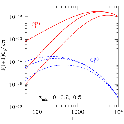
Figure 12: Predicted angular power spectra of the Compton y-parameter from the Poisson component (solid lines) and the correlation component (dashed) in the conventional $\Lambda$CDM model. Left: Contributions from clusters with masses lower than $M_{\rm max}=5\times 10^{15}$ (top), $5\times 10^{14}$ (middle), and $2\times 10^{14}$ (bottom) for $M_{\rm min}=10^{13}M_{\odot}$ and $z_{\rm min}=0$. Right: Contributions from clusters at redshifts higher than $z_{\rm min}=0$ (top), $0.2$ (middle), and $0.5$ (bottom) for $M_{\rm min}=10^{13}M_{\odot}$ and $M_{\rm max}=5\times 10^{15}M_{\odot}$. All the masses correspond to $M_{500}$.

The observed CMB power spectrum is dominated by primary anisotropies at $l\lower 2.15277pt\hbox{$\;\buildrel<\over{\sim}\;$}2000$ and by radio sources or dusty star-forming galaxies at higher multipoles (e.g., reichardt12 ; sievers13 ). Multi-frequency observations are hence crucial for separating the SZE power from the other components. Recent measurements of $C^{\rm yy}_{l}$ at $l\lower 2.15277pt\hbox{$\;\buildrel<\over{\sim}\;$}1000$ by Planck are in good agreement with the predictions similar to the one mentioned above planck_y . Contribution of the kinematic SZE is still uncertain and can arise from galaxy clusters aghanim98 ; molnar00 , spatial variations of the ionized fraction during cosmic reionization aghanim96 ; gruzinov98 ; knox98 , and density fluctuations in the reionized universe (also called the Ostriker-Vishniac effect) ostriker86 ; vishniac87 ; jaffe98 . The latter two components potentially provide a unique probe of the cosmic reionization history (e.g., zahn12 ).

Second, luminous galaxies are often used to trace clusters or groups of galaxies and their association with the thermal SZE have been studied by stacking the data toward a large sample of bright galaxies hand11 ; planck_group . A clear correlation is found between the stacked SZE flux and the stellar mass in the locally brightest galaxies selected from the Sloan Digital Sky Survey down to $M_{\rm star}\sim 10^{11}M_{\odot}$, corresponding to the effective halo mass of $M_{500}\sim 10^{13}M_{\odot}$ planck_group . The gas content of such low-mass halos is likely to account for a part of the missing baryon in the Universe fukugita98 .

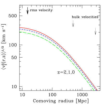
Figure 13: Linear theory predictions for the root-mean-square line-of-sight peculiar velocity over the comoving radius $r$ at $z=0$ (solid), $z=1$ (short dashed), and $z=2$ (long dashed) in the conventional $\Lambda$CDM universe. Thick and thin arrows mark the 2$\sigma$ upper limits on the rms velocity of massive clusters and the bulk velocities, respectively, measured by Planck planck_bulk .

Finally, large-scale coherent motion of the matter can be studied by means of the kinematic SZE. The linear perturbation theory predicts that the variance of line-of-sight peculiar velocities induced by surrounding density fluctuations is

$$\langle v_{\parallel}^{2}(r,z)\rangle=\frac{H_{0}^{2}E(a)^{2}a^{2}}{6\pi^{2}}\int_{0}^{\infty}\left(\frac{d\ln D}{d\ln a}\right)^{2}P_{\rm m}(k,z)|\tilde{W}_{r}(k)|^{2}dk,$$ (42)

where $\tilde{W}_{r}(k)=3[\sin(kr)-kr\cos(kr)]/(kr)^{3}$ is the 3D Fourier transform of the real-space top-hat filter over a comoving sphere of radius $r$. Figure 13 illustrates that the predicted root-mean-square (rms) velocity is $200\sim 300$ km s^-1 at $r=10$ Mpc corresponding to the enclosed mass of $M\simeq 2\times 10^{14}M_{\odot}$ and drops rapidly at larger radii with little redshift dependence at $z<2$. Note that numerical simulations suggest that the rms velocity of cluster-sized halos tends to be larger than the linear theory prediction by $20\sim 70\%$ (e.g. hamana03 ). While the kinematic SZE of this amount of velocity is hard to measure for individual clusters, a statistical detection of the mean pair-wise velocity has been reported using the ACT 148 GHz data for a sample of clusters and groups traced by 5000 luminous galaxies at $0.05<z<0.8$ hand12 . It has also been suggested that stacking the all-sky CMB data toward known galaxy clusters will give a measure of the bulk flow kashlinsky00 . Recent Planck data place $2\sigma$ upper limits on the rms radial velocity of $800$ km s^-1 for a sample of 100 massive clusters at $\langle z\rangle\sim 0.18$ and on the local bulk flow velocity of $250$ km s^-1 within $\sim 3$ Gpc planck_bulk as marked in Figure 13. While the limits are still weak, these measurements are consistent with predictions in the $\Lambda$CDM universe.

9 Summary

Extensive efforts well over four decades have now established the SZE as an indispensable tool in cosmology and astrophysics. Being one of the major foregrounds of the CMB, the SZE not only plays a key role in recovering correctly the primary anisotropies, but also offers unique cosmological tests on its own. They include measurements of the evolution of the CMB temperature, distances to high redshifts that are entirely free from the cosmic distance ladder, the absolute numbers and the power spectra of galaxy clusters, and large-scale motions of the Universe. It should be noted that their accuracy critically depends on our understanding of the physics of galaxy clusters and structure formation, which the SZE observations have also been improving, e.g., by finding high velocity cluster mergers, measuring pressure profiles, and detecting the gas in low-mass halos. Perhaps the most noticeable progress over the last decade or so is that the SZE measurements have started to achieve their own discoveries independently of any other means. This has made the SZE a truly complementary probe to X-ray observations in the studies of cosmic plasma. A number of outcomes from large area surveys and pointed observations by existing instruments are also underway. It is highly anticipated that future SZE measurements from both grounds and the space will continue to provide us new insights into our Universe.

References

- (1) Ya. B. Zel’dovich, and R. A. Sunyaev, Astrophys. Space Sci., 4, 301 (1969)
- (2) R. A. Sunyaev, and Ya. B. Zel’dovich, Comments Astrophys. Space Phys., 2, 66 (1970)
- (3) R. A. Sunyaev, and Ya. B. Zel’dovich, Comments Astrophys. Space Phys., 4, 173 (1972)
- (4) R. A. Sunyaev, and Ya. B. Zel’dovich, Mon. Not. R. Astron. Soc., 190, 413 (1980)
- (5) Z. Staniszewski, P. A. R. Ade, K. A. Aird, et al., \AJ701,32,2009
- (6) K. Vanderlinde, T. M. Crawford, T. de Haan, et al., \AJ722,1180,2010
- (7) R. Williamson, B. A. Benson, F. W. High, et al., \AJ738,139,2011
- (8) C. L. Reichardt, B. Stalder, L. E. Bleem, et al., \AJ763,127,2013
- (9) A. D. Hincks, V. Acquaviva, P. A. R. Ade, et al., Astrophys. J. Suppl., 191, 423 (2010)
- (10) T. A. Marriage, V. Acquaviva, P. A. R. Ade, et al., \AJ737,61,2011
- (11) M. Hasselfield, M. Hilton, T. A. Marriage, et al., J. Cosm. Astropart. Phys., 07, 008 (2013)
- (12) Planck Collaboration, Astron. Astrophys., 536, A8 (2011)
- (13) Planck Collaboration, arXiv:1303.5089
- (14) C. L. Reichardt, L. Shaw, O. Zahn, et al., \AJ755, 70, 2012
- (15) J. L. Sievers, R. A. Hlozek, M. R. Nolta, et al., J. Cosmol. Astropart. Phys., 10, 060 (2013)
- (16) Planck Collaboration, arXiv:1303.5081
- (17) N. Hand, J. W. Appel, N. Battaglia, \AJ736,39,2011
- (18) Planck Collaboration, Astron. Astrophys., 557, A52 (2013)
- (19) N. Hand, G. E. Addison, E. Aubourg, et al., \PRL109,041101,2012
- (20) J. Sayers, T. Mroczkowski, M. Zemcov, et al., \AJ778,52,2013
- (21) R. W. Schmidt, S. W. Allen, and A. C. Fabian, Mon. Not. R. Astron. Soc., 352, 1413 (2004)
- (22) M. Bonamente, M. Joy, S. J. LaRoque, J. E. Carlstrom, E. D. Reese, and K. S. Dawson, \AJ647, 25, 2006
- (23) E. De Filippis, M. Sereno, M. W. Bautz, and G. Longo, \AJ625, 108, 2005
- (24) M. Sereno, S. Ettori, and A. Baldi, Mon. Not. R. Astron. Soc., 419, 2646 (2012)
- (25) T. Kitayama, E. Komatsu, N. Ota, T. Kuwabara, Y. Suto, K. Yoshikawa, M. Hattori, and H. Matsuo, 2004, Publ. Astron. Soc. Japan, 56, 17
- (26) P. M. Korngut, S. R. Dicker, E. D. Reese, B. S. Mason, M. J. Devlin, T. Mroczkowski, C. L. Sarazin, M. Sun, and J. Sievers, \AJ734, 10, 2011
- (27) Planck Collaboration, Astron. Astrophys., 554, A140 (2013)
- (28) R. A. Sunyaev, and Ya. B. Zel’dovich, Annu. Rev. Astron. Astrophys., 18, 537 (1980)
- (29) Y. Rephaeli, Annu. Rev. Astron. Astrophys., 33, 541 (1995)
- (30) M. Birkinshaw, Phys. Reports, 310, 97 (1999)
- (31) J. E. Carlstrom, G. P. Holder, and E. D. Reese, Annu. Rev. Astron. Astrophys., 40, 643 (2002)
- (32) E. L. Wright, Astrophys. J. 232, 348 (1979)
- (33) R. Fabbri, Astrophys. Space Sci. 77, 529 (1981)
- (34) Y. Rephaeli, Astrophys. J. 496, 33 (1995)
- (35) A. Challinor, and A. Lasenby, Astrophys. J. 499, 1 (1998)
- (36) N. Itoh, Y. Kohyama and S. Nozawa, Astrophys. J. 502, 7 (1998)
- (37) S. Y. Sazonov and R. A. Sunyaev, Astrophys. J. 508, 1 (1998)
- (38) S. Nozawa, N. Itoh and Y. Kohyama, Astrophys. J. 508, 17, (1998)
- (39) N. Itoh, and S. Nozawa, Astron. Astrophys., 417, 827 (2004)
- (40) S. Nozawa, N. Itoh, Y. Suda, and Y. Ohhata, Il Nuovo Cimento B, 121, 487 (2006)
- (41) Planck HFI Core Team, Astron. Astrophys., 536, A6 (2011)
- (42) E. Audit, and J. F. L. Simmons, Mon. Not. R. Astron. Soc., 305, L27 (1999)
- (43) S. Y. Sazonov and R. A. Sunyaev, Mon. Not. R. Astron. Soc. 310, 765 (1999)
- (44) A. D. Challinor, M. T. Ford, and A. N. Lasenby, Mon. Not. R. Astron. Soc. 312, 159 (2000)
- (45) N. Itoh, S. Nozawa, and Y. Kohyama, \AJ533, 588, 2000
- (46) M. Kamionkowski, and A. Loeb, \PRD56, 4511, 1997
- (47) L. Feretti, G. Giovannini, F. Govoni, M. Murgia, Astron. Astrophys. Rev. 20, 54, (2012)
- (48) T. A. Ensslin, and C. R. Kaiser, Astron. Astrophys., 360, 417 (2000)
- (49) P. Blasi, A. V. Olinto, A. Stebbins, \AJ535, L71, 2000
- (50) S. Colafrancesco, P. Marchegiani, and E. Palladino, Astron. Astrophys., 397, 27 (2003)
- (51) D. J. Fixsen, \AJ707, 916, 2009
- (52) R. Fabbri, F. Melchiorri, and V. Natale, Ap&SS, 59, 223 (1978)
- (53) Y. Rephaeli, \AJ241, 858, 1980
- (54) L. Lamagna, E.S. Battistelli, S. De Gregori, M. De Petris, G. Luzzi, and G. Savini, New Astronomy Reviews, 51, 381 (2007)
- (55) J. A. S. Lima, A. I. Silva, and S. M. Viegas, Mon. Not. R. Astron. Soc., 312, 747 (2000)
- (56) G. Hurier, and N. Aghanim, M. Douspis, and E. Pointecouteau, Astron. Astrophys., 561, A143 (2014)
- (57) A. Saro, J. Liu, and J. J. Mohr, et al., arXiv:1312.2462
- (58) G. Luzzi, M. Shimon, L. Lamagna, Y. Rephaeli, M. De Petris, A. Conte, S. De Gregori, and E. S. Battistelli, \AJ705, 1122, 2009
- (59) J. N. Bahcall,, and R. A. Wolf, \AJ152, 701, 1968
- (60) S. Muller, A. Beelen, J. H. Black, S. J. Curran, C. Horellou, S. Aalto, F. Combes, M. Guelin, and C. Henkel, Astron. Astrophys., 551, A109 (2013)
- (61) P. Noterdaeme, P. Petitjean, R. Srianand, C. Ledoux, and S. López, Astron. Astrophys. 526, L7 (2011)
- (62) A. Cavaliere, L. Danese, G. de Zotti, \AJ217, 6, 1977
- (63) J. Silk, and S. D. M. White, \AJ226, 103, 1978
- (64) M. Birkinshaw, Mon. Not. R. Astron. Soc., 187, 847 (1979)
- (65) A. Cavaliere, L. Danese, G. de Zotti, Astron. Astrophys., 75, 322 (1979)
- (66) J. Uzan, N. Aghanim, M. Yannick, \PRD70,3533,2004
- (67) S. Sasaki, Publ. Astron. Soc. Japan, 48, L119 (1996)
- (68) U. Pen, New Astronomy, 2, 309 (1997)
- (69) H. Böhringer, and N. Werner, Astron. Astrophys. Rev., 18, 127 (2010)
- (70) S. Kobayashi, S. Sasaki, and Y. Suto, Publ. Astron. Soc. Japan, 48, L107 (1996)
- (71) J. F. Navarro, C. S. Frenk, S. D. M. White, \AJ490, 493,1997
- (72) F. De Bernardis, E. Giusarma, A. Melchiorri, Int. J. Mod. Phys. D, 15, 759 (2006)
- (73) R. Nair, S. Jhingana and D. Jain, J. Cosmol. Astropart. Phys., 05, 023 (2011)
- (74) V.F. Cardone, S. Spiro, I. Hook, and R. Scaramella, \PRD85, 123510, 2012
- (75) R. F. L. Holanda, J.A.S.Lima, and M. B. Ribeiro, Astron. Astrophys., 538, A131 (2012)
- (76) N. Suzuki, D. Rubin, C. Lidman, et al., \AJ746,85,2012
- (77) Y. Inagaki, T. Suginohara, and Y. Suto, Publ. Astron. Soc. Japan, 47, 411 (1995)
- (78) H. Kawahara, T. Kitayama, S. Sasaki, and Y. Suto, \AJ674, 11, 2008
- (79) E. D. Reese, H. Kawahara, T. Kitayama, N. Ota, S. Sasaki, and Y. Suto, \AJ721, 653, 2010
- (80) S. D. M. White, J. F. Navarro, A. E. Evrard, and C. S. Frenk, Nature, 336, 429 (1993)
- (81) R. S. Goncalves, R. F. L. Holanda, J. S. Alcaniz, Mon. Not. R. Astron. Soc., 420, L43 (2012)
- (82) S. J. LaRoque, M. Bonamente, J. E. Carlstrom, M. K. Joy, D. Nagai, E. D. Reese, and K. S. Dawson, \AJ652, 917,2006
- (83) K. Lancaster, et al., Mon. Not. R. Astron. Soc., 359, 16 (2005)
- (84) K. Umetsu, M. Birkinshaw, G.-C. Liu, et al., \AJ694, 1643, 2009
- (85) S. W. Allen, D. A. Rapetti, R. W. Schmidt, H. Ebeling, R. G. Morris, and A. C. Fabian, Mon. Not. R. Astron. Soc., 383, 879 (2008)
- (86) S. Ettori, A. Morandi, P. Tozzi, I. Balestra, S. Borgani, P. Rosati, L. Lovisari, and F. Terenziani, Astron. Astrophys., 501, 61 (2009)
- (87) A. Vikhlinin, R. A. Burenin, H. Ebeling, et al., \AJ692, 1033, 2009
- (88) Planck Collaboration, arXiv:1303.5076
- (89) A. Vikhlinin, A. Kravtsov, W. Forman, C. Jones, M. Markevitch, S. S. Murray, and L. Van Speybroeck, \AJ640, 691, 2006
- (90) Y.-Y. Zhang, N. Okabe, A. Finoguenov, et al., \AJ711, 1033, 2010
- (91) A. Simionescu, S. W. Allen, A. Mantz, et al., Science, 331, 1576 (2011)
- (92) D. Eckert, S. Ettori, S. Molendi, F. Vazza, and S. Paltani, Astron. Astrophys., 551, A23 (2013)
- (93) G. P. Holder, J. E. Carlstrom, and A. E. Evrard, In Constructing the Universe with Clusters of Galaxies, IAP 2000 meeting, eds. F. Durret, G. Gerbal, E45, 1 (2000)
- (94) T. Kitayama, S. Sasaki, and Y. Suto, Publ. Astron. Soc. Japan, 50, 1 (1998)
- (95) W. H. Press, and P. Schechter, \AJ187, 425, 1974
- (96) R. K. Sheth, and G. Tormen, Mon. Not. R. Astron. Soc., 308, 119 (1999)
- (97) A. Jenkins, C. S. Frenk, S. D. M. White, J. M. Colberg, S. Cole, A. E. Evrard, H. M. P. Couchman, and N. Yoshida, Mon. Not. R. Astron. Soc., 321, 372 (2001)
- (98) J. Tinker, A. V. Kravtsov, A. Klypin, K. Abazajian, M. Warren, G. Yepes, S. Gottlöber, and D. E. Holz, \AJ688, 709, 2008
- (99) M. Arnaud, G. W. Pratt, R. Piffaretti, H. Boehringer, J. H. Croston, and E. Pointecouteau, Astron. Astrophys., 517, A92 (2010)
- (100) Planck Collaboration, arXiv:1303.5080
- (101) B. A. Benson, T. de Haan, J. P. Dudley, et al., \AJ763,147,2013
- (102) A. Vikhlinin, A. V. Kravtsov, R. A. Burenin, et al., \AJ692, 1060, 2009
- (103) M. Kilbinger, L. Fu, , C. Heymans, et al., Mon. Not. R. Astron. Soc., 430, 2200, (2013)
- (104) A. Mantz, S. W. Allen, D. Rapetti, and H. Ebeling, Mon. Not. R. Astron. Soc., 406, 1759 (2010)
- (105) L. Wang, and P. Steinhardt, \AJ508, 483, 1998
- (106) E. V. Linder, \PRD72, 043529, 2005
- (107) D. Rapetti, C. Blake, S. W. Allen, A. Mantz, D. Parkinson, and F. Beutler, Mon. Not. R. Astron. Soc., 432, 973 (2013)
- (108) T. H. Reiprich, K. Basu, S. Ettori, H. Israel, L. Lovisari, S. Molendi, E. Pointecouteau, and M. Roncarelli, Space Sci. Rev. 177, 195 (2013)
- (109) J. Sayers, N. G. Czakon, A. Mantz, et al., \AJ768, 177, 2013
- (110) D. Nagai, A. V. Kravtsov, and A. Vikhlinin, \AJ668, 1, 2007
- (111) T. Plagge, B. A. Benson, P. A. R. Ade, et al., \AJ716, 1118, 2010
- (112) M. Bonamente, N. Hasler, E. Bulbul, et al., New Journal of Physics, 14, 025010 (2012)
- (113) Planck Collaboration, Astron. Astrophys., 550, A131 (2013)
- (114) Planck and AMI Collaborations, Astron. Astrophys., 550, A128 (2013)
- (115) K. Yoshikawa, and Y. Suto, \AJ513, 549, 1999
- (116) Q. Yuan, T.-J. Zhang, and B.-Q. Wang, Chin. J. Astron. Astrophys., 8, 671 (2008)
- (117) M. Nord, K. Basu, F. Pacaud, et al., Astron. Astrophys., 506, 623 (2009)
- (118) K. Basu, Y.-Y. Zhang, M. W. Sommer, et al. Astron. Astrophys., 519, A29 (2010)
- (119) D. Eckert, S. Molendi, F. Vazza, S. Ettori, and S. Paltani, Astron. Astrophys., 551, A22 (2013)
- (120) Y.-Y. Zhang, , A. Finoguenov, H. Böhringer, J.-P. Kneib, G. P. Smith, R. Kneissl, N. Okabe, and H. Dahle, Astron. Astrophys., 482, 521 (2008)
- (121) H. Kawahara, \AJ719, 1926, 2010
- (122) A. Morandi, M. Limousin, Y. Rephaeli, K. Umetsu, R. Barkana, T. Broadhurst, and Hakon Dahle, Mon. Not. R. Astron. Soc., 416, 2567 (2011)
- (123) M. Sereno, S. Ettori, K. Umetsu, and A. Baldi, Mon. Not. R. Astron. Soc., 428, 2241 (2013)
- (124) M. Markevitch, and A. Vikhlinin, Physics Reports, 443, 1 (2007)
- (125) E. Komatsu, H. Matsuo, T. Kitayama, M. Hattori, R. Kawabe, K. Kohno, N. Kuno, S. Schindler, Y. Suto, and K. Yoshikawa, Publ. Astron. Soc. Japan, 53, 57 (2001)
- (126) B. S. Mason, S. R. Dicker, P. M. Korngut, et al. \AJ716, 739, 2010
- (127) S. Schindler, M. Hattori, D. M. Neumann, and H. Böhringer, Astron. Astrophys., 317, 646, 655
- (128) S. W. Allen, R. W. Schmidt, and A. C. Fabian, Mon. Not. R. Astron. Soc., 335, 256 (2002)
- (129) T. J. Plagge, D. P. Marrone, Z. Abdulla, et al., \AJ770, 112, 2013
- (130) E. Komatsu, T. Kitayama, Y. Suto, M. Hattori, R. Kawabe, H. Matsuo, S. Schindler, and K. Yoshikawa, \AJ516, L1, 1999
- (131) M. Zemcov, C. Borys, M. Halpern, P. Mauskopf, and D. Scott, Mon. Not. R. Astron. Soc., 376, 1073 (2007)
- (132) E. Pointecouteau, M. Giard, A. Benoit, F. X. Désert, N. Aghanim, N. Coron, J. M. Lamarre, and J. Delabrouille, \AJ519, L115, 1999
- (133) E. Pointecouteau, M. Giard, A. Benoit, F. X. Désert, J. P. Bernard, N. Coron, and J. M. Lamarre, \AJ552, 42, 2001
- (134) E. D. Reese, J. E. Carlstrom, M. Joy, J .J. Mohr, L. Grego, and W. L. Holzapfel, \AJ581, 53, 2002
- (135) B. A. Benson, S. E. Church, P. A. R. Ade, J. J. Bock, K. M. Ganga, C. N. Henson, and K. L. Thompson, \AJ617,829,2004
- (136) M. Zemcov, J. Aguirre, J. Bock, et al., \AJ749, 114, 2012
- (137) N. Ota, , K. Murase, T. Kitayama, E. Komatsu, M. Hattori, H. Matsuo, T. Oshima, Y. Suto, and K. Yoshikawa, Astron. Astrophys., 491, 363 (2008)
- (138) M. Gitti, C. Ferrari, W. Domainko, L. Feretti, and S. Schindler, Astron. Astrophys., 470, L25 (2007)
- (139) C. Ferrari, H. T. Intema, E. Orru, et al., Astron. Astrophys., 534, L12 (2011)
- (140) F. Menanteau, J. P. Hughes, C. Sifon, et al., \AJ748, 7, 2012
- (141) K. Yamada, T. Kitayama, S. Takakuwa, et al., Publ. Astron. Soc. Japan, 64, 102 (2012)
- (142) S. Cole, and N. Kaiser, Mon. Not. R. Astron. Soc., 233, 637 (1988)
- (143) R. Schaeffer, and J. Silk, \AJ333, 509, 1988
- (144) M. Markevitch, G. R. Blumenthal, W. Forman, C. Jones, and R. A. Sunyaev, \AJ395, 326, 1992
- (145) N. Makino, and Y. Suto, \AJ405, 1, 1993
- (146) J. G. Bartlett, and J. Silk, \AJ423,12, 1994
- (147) D. N. Limber, \AJ117, 134, 1953
- (148) E. Komatsu, and T. Kitayama, \AJ526,L1,1999
- (149) H. J. Mo, and S. D. M. White, Mon. Not. R. Astron. Soc., 282, 1096 (1996)
- (150) E. Komatsu, and U. Seljak, Mon. Not. R. Astron. Soc., 336, 1256 (2002)
- (151) G. Efstathiou, M. Migliaccio, Mon. Not. R. Astron. Soc., 423, 2492 (2012)
- (152) N. Aghanim, S. Prunet, O. Forni, and F. R. Bouchet, Astron. Astrophys., 334, 409 (1998)
- (153) S. M. Molnar, and M. Birkinshaw, \AJ537, 542, 2000
- (154) N. Aghanim, F. X. Desert, J. L. Puget, and R. Gispert, Astron. Astrophys., 311, 1 (1996)
- (155) A. Gruzinov, and W. Hu, \AJ508, 435, 1998
- (156) L. Knox, R. Scoccimarro, and S. Dodelson, \PRL81,2004,1998
- (157) J. P. Ostriker, and E. T. Vishniac, \AJ306,L51,1986
- (158) E. T. Vishniac, \AJ322,597,1987
- (159) A. H. Jaffe, and M. Kamionkowski, \PRD58, 043001, 1998
- (160) O. Zahn, C. L. Reichardt, L. Shaw, et al. \AJ756,65,2012
- (161) M. Fukugita, C. J. Hogan, and P. J. E. Peebles, \AJ503, 518, 1998
- (162) T. Hamana, I. Kayo, N. Yoshida, Y. Suto, and Y. P. Jing, Mon. Not. R. Astron. Soc., 343, 1312 (2003)
- (163) A. Kashlinsky, and F. Atrio-Barandela, \AJ536, L67, 2000
- (164) Planck Collaboration, Astron. Astrophys., 561, A97 (2014)