Execution Time Analysis for Industrial Control Applications

Abstract

Estimating the execution time of software components is often mandatory when evaluating the non-functional properties of software-intensive systems. This particularly holds for real-time embedded systems, e.g., in the context of industrial automation. In practice it is however very hard to obtain reliable execution time estimates which are accurate, but not overly pessimistic with respect to the typical behavior of the software.

This article proposes two new concepts to ease the use of execution time analysis for industrial control applications: (1) a method based on recurring occurrences of code sequences for automatically creating a timing model of a given processor and (2) an interactive way to integrate execution time analysis into the development environment, thus making timing analysis results easily accessible for software developers. The proposed methods are validated by an industrial case study, which shows that a significant amount of code reuse is present in a set of representative industrial control applications.

1 Introduction

Calculating the execution time for a given piece of code on a modern processor is a very difficult problem. In most cases, an accurate solution is impossible to find because it relates to the halting problem which is undecidable. In real-time systems, however, calculating the longest time a piece of code might take to execute (Worst-Case Execution time, WCET) is necessary to verify that all real-time requirements are met. To obtain an estimate for the WCET despite its general undecidability, approximation techniques must be used. There are two main approaches to approximate the WCET of a software component: Testing or in-situation profiling of a piece of code can be used to measure the execution time of diverse executions. The WCET of the respective code can then be estimated from these measurements through heuristics. Alternatively, static code analysis techniques can be used to calculate the WCET using a model of the hardware.

The first approach requires that sufficient code coverage can be achieved during the measurements and that the worst-case execution time for every program statement has been observed. In practice, these requirements cannot always be fulfilled and therefore the WCET might be under-approximated. The second approach, static WCET analysis, requires the manual development of a hardware model for the target processor, which estimates the execution time based on formal methods. This is a long and costly process, as it requires the efforts of highly specialized software developers for multiple person months. The abstraction underlying the model approximates the execution time in a conservative fashion, thereby leading to an over-approximation of the actual WCET. On the positive side, the resulting WCET estimate can be safely applied in systems with hard real-time requirements, as it is guaranteed to be an upper bound for every possible execution time of the program.

Besides the manual development of the timing model for the hardware, the integration of the execution time estimates into the development process of software with real-time constraints is another challenge. The time a piece of software requires to execute on a specific processor can be expressed with one or more of the following three values: best-case execution time (BCET), worst-case execution time (WCET) and average-case execution time (ACET). Existing static analysis tools only approximate the best-case and worst-case execution time, usually by determining an upper or lower bound for the possible execution times of a program. As the interaction and interdependence between program parts is only approximated, the resulting estimates often contain execution paths through the program which are infeasible in practice. The abstraction underlying these estimates can both hide the semantics of the programs and the execution time estimates can deviate significantly from the average execution time observable during measurements.

The problem with determining only an upper and lower bound for the execution time is that this information is of little use for software developers of soft real-time or non-real-time systems. For this usage scenario, the average-case execution time is more relevant. Today, a large number of program runs has to be observed and measured in order to determine an accurate average-case estimate or a good approximation of the execution time distribution from measurements. Such average-case execution time estimates can only be determined if hardware with measurement or profiling capabilities is available during software development. There is however no established method and no established tool for reasoning about average-case execution time without observing actual program executions.

This paper proposes two new concepts to facilitate the use of execution time analysis during software development for real-time applications. The techniques were originally developed for industrial control applications, but are equally applicable in other domains with (soft) real-time requirements. Section 2 introduces related work on worst-case execution time analysis. Section 3 of this paper proposes a method to automatically create a timing model for a given processor based on the repeated occurrence of code patterns resulting from model-based code generation. In Section 4, an interactive way to integrate execution time analysis into the development environment is described, thereby improving the interaction between timing analysis tools and software developers. In Section 5, preliminary results validating the applicability of the proposed approach are presented. Finally, Section 6 summarizes the paper and gives an outlook.

2 State of the Art in Execution Time Analysis

As mentioned in the previous section, execution time estimation techniques can be classified according to the way the estimates are determined. Static techniques use a structural analysis of a piece of software and an analytical model of the underlying hardware to determine execution time estimates without executing the software. On the other hand, dynamic techniques require executing the program of interest in order to estimate the execution time of a program. Furthermore, some dynamic estimation techniques also use a (static) structural analysis of a program when estimating its execution time. Both types of techniques are explained in detail in the following paragraphs.

2.1 Static Timing Analysis

Figure 1: Example of code

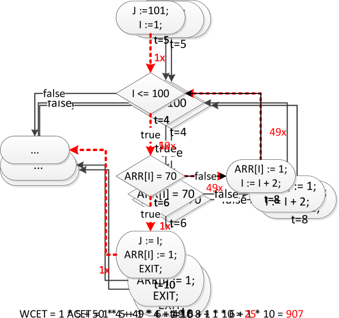
Figure 2: Extracted control flow

Static timing analysis techniques estimate the execution time of a program without actually executing any code. They are mainly used to determine the WCET of a program, meaning a conservative estimate or upper bound for the execution time of a program. Most existing solutions are based on static program analysis techniques to model the execution of a piece of software on a given target processor [15]. They can be roughly decomposed into the following three steps (see Figure 1 to Figure 4):

1. Control flow analysis decomposes the structure of the program into atomic units for the subsequent analysis steps. The resulting program representation is usually the control flow graph (CFG) of the program, which consist of basic blocks. A basic block is a maximal sequence of program statements with only one point of entry and exit. For the example in Figure 1, the resulting CFG is shown in Figure 2.

2. Micro-architectural analysis determines the execution time for the atomic units of a program using the result of the control flow analysis. In most cases this analysis is performed using an abstract model of the target processor. This model can be based on abstract interpretation [14] or symbolic execution [10]. In both cases the model focuses on the execution time for sequences of machine instructions and can neglect details of the computations these instructions would perform on the real hardware. This abstraction is necessary to make the estimations computationally feasible, but it can also be the source of imprecision. The reason for this is the way the micro-architectural analysis deals with information about the system state which is not available due to abstraction: whenever the analysis cannot prove that certain effects which impact the execution time, e.g., cache misses, will never occur at a certain program point, it will assume the system state leading to the longest execution time. Depending on how much abstraction is necessary to cope with complexity of the internal state of the processor, this can entail a large number of pessimistic assumptions and thus a large overestimation of the WCET. An example for the outcome of this analysis step is shown in Figure 3 by annotating execution times to the CFG from Figure 2. Time units are omitted for this example, but most existing tools use CPU clock cycles.

3. Global bound calculation uses the results of the two previous steps to obtain an estimate for the total execution time of a program. The prevalent technique for doing this is implicit path enumeration [8]. This approach translates the structural constraints and local execution time estimates into an integer linear programming (ILP) problem, which is then solved using standard ILP solvers. If a program contains loops, the maximal number of times a loop may execute must be determined by a previous analysis or provided by the user. This is necessary for the ILP solver to find a worst-case path. The loop in the example from Figure 1 can be executed at most 50 times. Thus, the edge leaving the basic block checking the loop condition can be taken at most 50 times on any execution path of the program. With this structural information and the cost associated with each basic block, the global bound analysis will identify the worst-case path, as shown using dotted lines in Figure 4. This path assumes that the maximal number of loop iterations is executed and that the conditional statement in line 3 of Figure 1, which aborts the loop, will be executed in the 50th iteration of the loop.

Figure 3: Result of Micro-architectural Analysis

Figure 4: Result of Global Bound Calculation

Existing static timing analysis tools are able to estimate the best-case or worst-case execution time of software components. Estimating an average-case execution time is usually not supported. Moreover, the challenge with static timing analysis is the creation of the required abstract processor models. Currently, these models are developed manually by the tool vendors, which is a tedious, costly and error-prone process. For simple processor architectures, static WCET analysis can estimate execution times with an error rate of less than 10%. However, this high level of accuracy can only be achieved if the program path predicted by the WCET analysis roughly matches the execution path observed during the measurement runs [17]. For simple processor architectures with simple pipelines and without caches, the third step, global bound calculation, is therefore the most likely phase to introduce an overestimation. On the other hand, for processors with multi-level caches and multiple cores, the micro-architectural analysis can also introduce a lot of pessimism to the execution time estimates as internal state of the processor must be approximated conservatively. Consequently, the obtainable accuracy of the execution time estimates reported by static WCET analysis tools is likely to show even higher error rates for more complex processor architectures.

2.2 Dynamic Timing Analysis

With dynamic timing analysis, the execution time of software is measured directly on the hardware. This means that target hardware must be available. The level of granularity at which these measurements can be performed varies for different processor architectures. While most current processor architectures support hardware performance counters, these counters can only provide a limited level of accuracy and care must be taken in order to obtain accurate measurements [16]. Moreover, it might be necessary to modify the observed program by adding instrumentation code for manipulating the hardware performance counters of the processor. Modifying the program code can obviously impact the measurements. To perform measurements with an increased level of accuracy, e.g., up to the level of individual instruction, additional tools like logic analyzers or processors with dedicated tracing hardware support are required.

Probabilistic and statistical timing analyses [3] are variants of dynamic approaches for execution time estimation. Probabilistic timing analysis tries to capture the variance of execution times by providing a probability distribution for the possible execution times of a program. This distribution is calculated by analyzing the execution time of individual program parts from a large set of measurements. The complete measurement process can take several days of observing the system in operation and produce gigabytes of data. Using this data, the execution time distributions of smaller program parts are incrementally combined to get the distribution for the complete program. The limitation of this combination step is that the execution time of individual program parts is assumed to be independent, which is often not the case in practice. More recent approaches for dynamic timing analysis apply statistical methods, like extreme value theory, to reason about the worst-case execution of a program without ever observing it [9]. However, this is still an area of active research without a generally accepted solution.

2.3 Integration into the Development Process

In some application domains, e.g, avionics or automotive, worst-case execution time analysis is standard practice during software development to verify that real-time requirements are met. Special software development tools and languages used in the automation domain often prevent the use of tools from other domains. Additionally, the real-time requirements can be slightly different. On the one hand, there are hard real-time boundaries for the execution time of control applications which are defined by their cyclic activation. On the other hand, it is acceptable that these deadlines are missed sometimes as long as this does not happen repeatedly. This can happen if an isolated event, which is not part of the typical execution path, requires some special handling in the code. Examples for this are the execution of initialization code during startup or the creation of status messages. Since the system design can handle this application behavior, missing an execution deadline for other reasons, like an increased execution time due to cache misses, is less critical than in other application domains which require guaranteed upper bounds for the execution time of software components. However, WCET estimates reported by existing analysis tools only consider the theoretical worst-case execution path through a program, which is executed very rarely (or not at all) for typical control applications. If the WCET is used to characterize the CPU load of a control device, this leads to a significant waste of computing resources.

A static analysis technique for average-case execution time would be a viable alternative. Finding the typical execution path through a program requires execution of the program or additional manually provided information about the expected behavior of the program. The latter is currently not done in any solution. Furthermore, the potential variation between the best-, average-, and worst-case execution times is an important piece of information which should be made available as a result of an execution time analysis. Currently, there is no system or tool which can reason about this variation in a static way, meaning a way which does not require the execution of the program of interest.

3 New Approach: Timing Model Generation for Control Applications

A major hurdle for estimating the execution time of cyclic real-time control applications is that, in the current development process, these estimates can only be made as soon as an industrial control device (controller) is available. Static timing analysis tools are currently not available for all the processor variants. Consequently, the CPU load on the device can only be determined after the control applications have been developed and deployed to hardware. The load is defined as

$$\mathit{load}=\frac{\mathit{application~{}execution~{}time}}{\mathit{periodic~{}activation}}$$

The periodic activation depends on the production process being regulated by the control logic, meaning how often the application has to check inputs and adjust adjust. Knowing the expected load early, i.e., already during application development is beneficial for two reasons: As there is a direct correlation between the processing power of a controller and its cost, it is very desirable to choose a hardware variant which matches the application requirements without being overbuilt. Moreover, with a foreseen increase of distributed or parallel execution of applications, information about the execution time of individual program parts helps in tailoring the control application to its execution environment, e.g., through efficient partitioning of an application on a controller with a multi-core processor. To achieve this, execution time estimation must be an integral part of the software development process.

3.1 Timing Model Generation Flow

The intention of the proposed approach is to replace the currently used abstract, but complete models of CPU timing behavior with a model which only covers those instruction sequences which are actually used by programs in the targeted domain. This approach can significantly reduce the cost for developing such models and also makes them applicable in domains with less strict requirements. In contrast to similar work presented in [2], the proposed technique is not intended to generate a general purpose timing model for arbitrary applications. A similar idea for reusing WCET estimates has already been presented in [4], but the approach presented in this work aims at a reuse at a more fine-grained level.

To accurately estimate the best-, average- and worst-case execution time of a software component without requiring its execution to be observed, a timing model for the processor executing the software must be available. The execution time of a sequence of machine instructions greatly depends on how these instructions move through the pipeline and the functional units of the processor and how their execution can be interleaved. The execution time of individual instructions, e.g., from the processor manual or from repeatedly measuring the execution of the same instruction type, can only serve as a starting point for estimating the execution time of a complete program. On the other hand, the way machine code for control application is generated, e.g, when using ABB’s family of Control Builder tools or similar model-based tools allows the reasonable assumption that certain sequences or patterns of instructions occur repeatedly. Thus, in contrast to known static analysis methods, a general model of the processor pipeline might not be needed to obtain reasonably accurate performance estimates for control applications.

This insight motivates using their domain-specific properties to characterize the execution time of control applications based on recurring code sequences. The basic idea is to

1. automatically extract recurring code sequences from a set of training applications and

2. to use automatic test data generation techniques to determine their on-target execution time.

Thereby, a timing model for the CPUs used in industrial control devices can be generated with acceptable effort. Still, this model provides sufficient timing accuracy. The timing model, i.e., the contained timing information about recurring code sequences, then is used to determine the execution time of control applications with a similar structure. Moreover, the model is also applicable to applications that are created using the same set of tools. This approach is thus an alternative to the current practice of manually developing timing models, e.g., as used in commercial tools for static timing analysis.

The proposed timing model generation work flow is shown in Figure 5. An initial timing model of a CPU is constructed by considering single instructions only in step 1. This initial model should at least contain best-case and an worst-case execution time estimates for every instruction type of the CPU for the target controller. This information can be extracted from the CPU data sheet or by using synthetic benchmarks to measure the execution time of a single instruction type. This step has to be repeated for every new CPU variant used in an industrial controller. The resulting instruction-level estimates could already be used to automatically determine coarse-grained performance estimates for every control application as long as the occurrence of individual machine instructions can be counted.

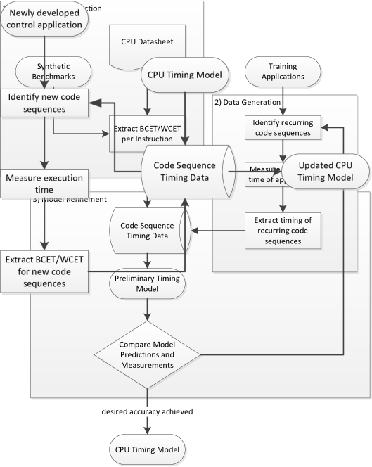
Figure 5: Timing Model Construction

Subsequent to the creation of the baseline model, which only considers individual instructions, data to create the timing model of the CPU is created using a set of control applications to train the model, as shown by step 2 of Figure 5. This refinement is done by extending the timing model to longer sequences of machine instructions. The training applications are decomposed into smaller code pieces which are searched for recurring code sequences. For these recurring sequences, more precise estimates are obtained by performing detailed measurements of the respective program parts. To allow for estimating variations in the execution time of a program, the implementation must be able to track the execution time triple of each code sequence, meaning the best-case, the average-case and the worst-case execution times. Ideally, the model should not only consider the execution time of code sequences in isolation, but also their interleaving and interdependence. That is, if the execution time of a code sequence A is influenced by the fact that code sequence B is executed in advance, this information is also considered by the model. After the timing model has been created automatically, standard static analysis techniques can be used to determine the possible execution of an arbitrary control application. The structure of the control application has to be decomposed into code sequences for which the timing model can provide execution time estimates. If no information for longer code sequences is available in the timing model, it might be necessary to decompose the program up to the level of individual machine instructions. The latter case is always possible and can make use of the information from the baseline model. Using the timing model created by the proposed approach, the execution time of newly developed applications can be performed through a bottom-up accumulation of execution times of recurring code sequences, e.g., based on the control flow graph of the program. The process of finding recurring code sequences and characterizing their execution time will be described in the following paragraphs. The model refinement continues until the predictions of the generated model fulfill the desired timing accuracy (step 3 in Figure 5), which can be checked by comparing the predictions of the model to end-to-end execution time measurements of the training applications.

3.2 Finding Recurring Code Sequences

The fundamental requirement for the proposed timing model generation is that recurring code patterns exist in the application code and that these patterns can be detected automatically. Code clone detection techniques are a natural choice to detect these patterns in the machine code. However, most code clone detection techniques work at the source code level, although there are publications dealing specifically with binary code [13]. The simplest form of searching for recurring code sequences is by looking for verbatim copies. For source code, this would mean searching for identical character sequences in the source code, but discarding white space. The binary-level equivalent for this approach would be to search for sequences in the machine code which are identical down to the last bit.

As two pieces of code with the same origin and identical functionality do not have to be completely isomorphic, e.g., due to some renaming of variables in the source code or using different registers for the same machine code operations, code clone detection techniques usually apply different forms of normalization to the analyzed program. For code clone detection at the machine code level, normalization techniques include discarding the order of instructions, abstracting the opcodes into certain classes, or translating the arguments of machine code operations into a symbolic form. These normalization techniques are applied to certain code areas, e.g., instruction sequences of a fixed length. The result can be a vector of attributes, for instance a vector containing number of instructions with a given opcode, or a hash value of the normalized instruction sequence. This normalized representation can be used to efficiently compare code areas to detect similar code areas and thus, (potential) code clones.

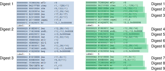
Figure 6: Basic Block and Window-Based Digest Computation

For the purpose of characterizing the execution time of recurring code sequences there are several constraints for applying known normalization techniques: The order of machine instructions should not be discarded as the execution order has a significant impact on execution time. The same holds for operands of an instruction, but to a lesser extent. To simplify the detection of recurring code sequences, the detection algorithm focuses on sequences of instruction opcodes only. Thus, an MD5 hash for the opcodes within basic blocks is computed and used as normalized characterization of the application code. For a given sequence of machine instructions, including their address, input registers and intermediate constants, only the opcode of the instruction is used for computing the MD5 digest of the sequence. Basic blocks can be further decomposed when searching for recurring sequences, but the sequences used for clone detection cannot span multiple basic blocks. Therefore each considered sequence can contain at most one branch instruction.

Different granularities for the computation of digests are illustrated in Figure 6. The machine code shown was generated by ABB’s engineering tool Compact Control Builder, which is used to develop control applications. For the most coarse-grained variant on the left side, all instructions of a basic block are used directly. This means that the value of Digest 1 is computed by applying the MD5 hash function to the opcode sequence (mflr, stwu, stw, lwz, lwz, lwz, cmpwi, bc). For all other basic blocks, which are marked with a label in the code, the digest is computed in the same way.

For a more fine-grained characterization, digests can be calculated using a sliding window approach which splits up the basic blocks in the machine code. To generate instruction sequences from a basic block, sequences are determined by moving a window of fixed size across the basic block using a fixed stride. This is illustrated in the right-hand part of Figure 6 using a window size of 4 instructions and a stride of 2 instructions. For Digest 1, the hash value of the opcode sequence (mflr, stwu, stw, lwz) is computed. The stride value can only be less than or equal to the window size, because otherwise not all instructions from the basic block would be included. Choosing the stride value smaller than the window size makes it more likely to capture recurring sequences. At the end of a basic block, the window size is pruned if it would otherwise move across the end of the basic block. For the last window of this example, the window size is pruned and thus Digest 9 is computed only from the single opcode blr.

After the training applications for timing model generation have been partitioned into digests, the digest values can be used to detect recurring code sequences. The underlying assumption is that sequences with identical digests will have identical execution times. To reduce the measurement effort needed to characterize the execution time of the recurring sequences, the number of sequences contained in the timing model should be as small as possible. On the other hand, the model should contain enough instruction sequences so it is rarely necessary to fall back to the single instruction baseline model when characterizing the execution time of a newly developed control application. This trade-off is still under investigation. Preliminary results on how to detect the recurring code sequences for an accurate and minimal timing model are presented in section 5.

3.3 Timing Characterization

Determining the execution time of recurring code sequences poses several challenges. First of all, it must be possible to measure the execution time of relatively short instruction sequences. On most modern processor architectures, this is only possible by adding instrumentation code. When characterizing the execution time of recurring code sequences, there is obviously a trade-off between the effort needed to perform the measurements and the accuracy of the characterization. In particular the overhead added to measurements by adding instrumentation code has to be considered. Based on our initial evaluation, the most suitable framework for implementing this part of our proposed work flow is the Dyninst binary instrumentation infrastructure [11], as it provides static instrumentation capabilities which do not add virtualization overhead to the measurements. A prototype tool based on Dyninst is currently being implemented.

Another challenge for the timing characterization is observing all relevant execution times. This will be tackled by extensive testing during model generation. One option is to use the existing test cases for the training applications from which the timing model is generated. As the main purpose of such test cases is not the generation of a CPU timing model, additional tests will be necessary. It is planned to apply automatic test case generation techniques. Thus, approaches like random or concolic testing [6, 12] will be used to generate input data for the measurements in the final implementation of the proposed approach. The recently introduced concept of micro execution [5] to test small portions of binary code with arbitrary inputs might also be applicable.

The important difference between the proposed work flow and existing measurement-based timing analysis tools is that timing measurements have to be performed only once per target processor and not once per application. The effort for setting up a test environment and measurement facilities will therefore only be needed once. The execution time measurements are formalized by applying sophisticated test case generation techniques. Furthermore, it is not necessary that the user of the resulting timing model has access to the target hardware to generate timing estimates for a newly developed application. The second important property is the integration of average-case execution times for the recurring code sequences into the model. This allows reasoning about the average load of the targeted device without running the software on the actual hardware. To achieve this, the model must store the best-case, the average-case and the worst-case execution time for each recurring code sequence.

4 Execution Time Estimation with User Feedback

In order to present the information about the execution time to the developer and to allow a fine-grained consideration of the program structure in the execution time analysis, a tight integration into the software development environment is crucial. An approach for integrating WCET estimates into a code editor to give the software developer feedback about the execution time of a program has been presented in [7]. By contrast, the approach presented in this paper makes the possible variation in the execution time of a software component explicit and thus enables the developer to make more accurate decisions whether all real-time requirements of the application can be met under the expected conditions.

After a timing model has been created for a target processor using a set of training applications, the resulting model can be used to estimate the execution time of newly developed applications. Thus, it could serve as a replacement for the micro-architectural analysis of existing analysis tool chains described in section 2.1. However, our approach might still lead to overly pessimistic execution time estimates due to incorrectly approximated program control flow. Nonetheless, the previously described approach for an automatic timing model generation overcomes the need for additional measurements and access to hardware during software development, while the effort for developing a timing model is reduced.

To facilitate the use of the timing model, we propose a 3-valued representation of the potential execution times. This directly presents the application’s ACET, BCET and WCET to the user. Thereby, the user is much better informed about the application’s potential behavior already in the development phase and additionally gets direct feedback on application changes. A mock-up of how this could look like is shown at the bottom of Figure 7. In addition to giving feedback to the user, the average-case execution time estimate can be significantly improved by only considering parts of the application which are included in a typical execution. Therefore, the user has to provide the required insights about the expected or typical program path—which often can be done due to the user’s experience and knowledge of the application. In combination with the previously described ACET estimates for recurring code sequences and structural program information, a more accurate approximation of the typical case can be achieved. The reason for this is that execution time outliers are less likely to impact the result of the average-case estimate. The standard way of simply averaging the executing time of observed program runs to get an ACET estimate would still include such outliers, but the proposed approach allows excluding such atypical executions. Finally, the 3-valued representation of the execution times still makes the worst case explicit to the user and thus, no information is lost compared to a standard WCET analysis.

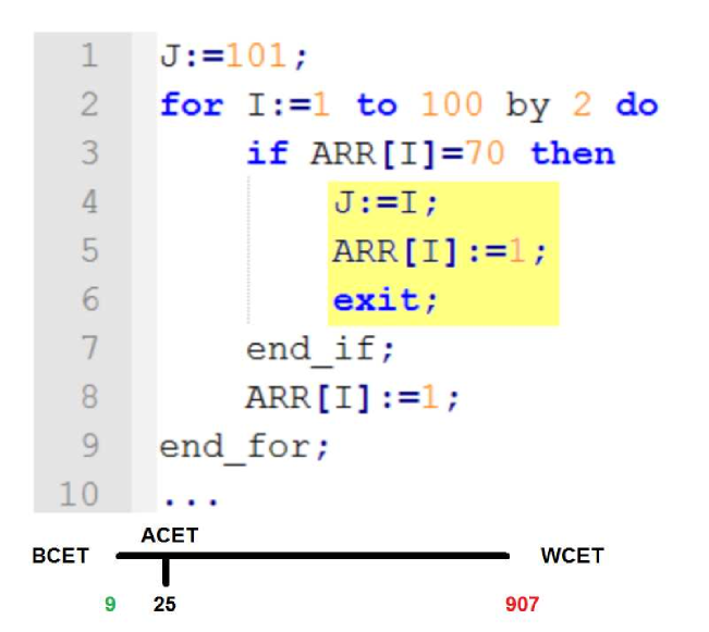
Figure 7: Typical Execution Marked

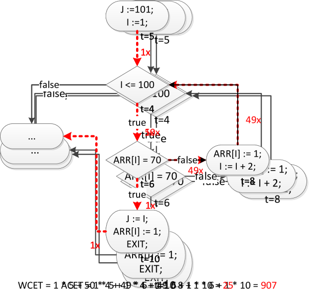
Figure 8: Typical Case Execution Time Estimation

The example program from section 2.1 will be used to illustrate the application of user feedback in estimating execution times. If we assume that the programmer of the code shown in Figure 7 knows that conditional expression in the loop typically evaluates to true immediately, she can mark the respective code area as being part of the typical execution. This is illustrated in Figure 7 by shading the respective code area. A similar tagging functionality could be easily added to any code editor. While this is an artificial example, similar patterns can often be found in control applications, e.g., for initialization code. By automatically translating this information into constraints for the global bound calculation analysis step, it can be used to restrict the program paths through the CFG. Thus, the program path determined by the global analysis for the ACET step no longer considers the worst-case path, but the typical path. The resulting program path for the example is shown in Figure 8. The edges drawn as dotted lines and the frequency annotations next to them describe the typical path. Consequently, each of the basic blocks along this path is executed exactly once. Using this information and the execution time of each basic block, which is also annotated to the CFG in Figure 8, an ACET of 25 cycles can be derived. The respective ACET formula is shown in the lower portion of Figure 8. Even if there is only small difference between the average-case and the worst-case execution time of the basic blocks, considering information about the typical program path can still reduce the overestimation of static timing analysis. While existing WCET analysis tools already support similar path constraints, the underlying timing model is always a pure worst-case analysis.

The combination of the ACET estimates and the user-provided information about the typical program path allows for characterizing the typical execution time of programs more accurately than with existing solutions. Thus, it goes beyond classical BCET and WCET analysis. Since the results of the WCET and BCET analysis are still represented, the information is still available to the user of the timing analysis. Adding average-case information allows to additionally reason about the load of a computer system by considering typical execution paths only. The proposed approach depends, however, on the user’s correct knowledge on the typical execution path. Thus, we are planning to case-study the quality of user input and the impact of wrong assumptions, e.g., mistakenly unmarked typical code areas or wrongly marked code areas, on calculated ACET estimates with real industrial applications and users.

The 3-valued execution time estimation can be applied at different levels of granularity, e.g., complete applications, components, or individual source code lines. We envision an integration of this representation into the integrated development environment for the developers of control applications. This is illustrated in the lower portion of Figure 7. By integrating this representation into the application development environment, the contribution of individual program parts is directly presented to the application developer. Thereby the 3-valued representation makes the possible variation of execution times explicit to the developer. In addition, program parts with a high contribution to the execution time are highlighted directly if the 3-valued execution time estimate is represented at the level of basic blocks or individual code lines. To adapt the 3-valued execution time estimate, the developer can mark program areas as being not part of a typical execution. This will exclude the respective program parts from the average-case execution time estimate. Alternatively, the offending program parts can be optimized manually by the developer and the 3-valued estimate can instantly provide information about the impact of the code changes on the execution time.

In the context of industrial control applications, code portions which belong to an atypical execution path can often be identified automatically. The result of a certain firmware function directly relates to whether the controller is in a typical state or not. For instance in most executions of a control application, the firmware function which checks whether the device just experienced a warm restart will return false. Thus, when the respective function is used in a conditional expression, this can be directly translated into a constraint for the average-case analysis. When performing a worst-case analysis, these constraints should of course not be used as they might lead to an underestimation of the WCET.

Essentially, marking certain code areas as the typical execution path excludes alternative paths from the WCET analysis and thus approximates the expected behavior more accurately. Depending on the application for which the execution time is estimated, the user-provided information could also be used to tag code areas for other scenario-based analyses. This allows for a more accurate estimation of the execution time under certain preconditions. The proposed approach could therefore also be extended for analyzing the execution time of a program under specific operating conditions.

5 Experimental Results

This section presents preliminary results for the proposed timing model generation work flow. The prototyping was carried out using the machine code output facilities of ABB’s Compact Control Builder development tool targeting the ABB AC 800M controller family. The basic block and window-based hash computation described in Section 3.2 were applied to three real-world Compact Control Builder projects to evaluate the amount of code sharing across different applications.

Each project contained multiple control applications which shared some code through common libraries. However, these libraries are always reused as source code, not as compiled machine code. Binary-level code sharing was analyzed by first calculating all possible digests for a fixed calculation technique for two of the three projects. All of the possible digests were stored in a database. Then all possible digests of the remaining project were computed and compared to the information stored in the database. The outcome of this experiment is shown in Table 1 for the basic block digest computation and window-based digest computation using a window size of 8 and 16 instructions. The size of each project is given in terms of instructions in the machine code after compilation. If certain modules were reused across different applications in the same project, the respective machine instructions were only counted once. The detection of recurring code patterns across the different projects could be executed in a few minutes on a standard laptop computer. Since the analysis tools is a very early prototype, no detailed performance measurements were conducted.

		Basic Blocks		Window=16, Stride=8		Window=8, Stride=4
Project ID	Size	Recurring Patterns	Instruction Coverage	Recurring Patterns	Instruction Coverage	Recurring Patterns	Instruction Coverage
Project 1	53028	3024	54.13%	5902	82.50%	12634	94.34%
Project 2	545328	14593	65.16%	64058	88.22%	134097	97.55%
Project 3	119546	4309	62.51%	14213	87.35%	29634	97.37%

Table 1: Clone Detection Granularity

The number of recurring code sequences was calculated by counting the number of hash digests a project has in common with the two remaining projects. So the numbers given in each line of the table show how much recurring code patterns where found in the respective project when the other projects where used as training data. Besides counting the number of recurring code sequences for the respective clone detection granularity, the second result column for each variant contains the percentage of machine instructions covered by these sequences. This value is calculated by dividing the number of machine instructions within a project which are included in recurring code sequences by the total number of instructions in the project. The rationale behind this estimation is that it determines the maximal achievable coverage if all recurring code sequences of the respective granularity would be part of the timing model.

The instruction coverage is relevant since it is not only an indicator of how much code sharing between different projects could be detected, but also what amount of code was not covered by any of the recurring code sequences. For the proposed automatic timing model generation, the number of recurring code patterns covered by the model should be minimal, while the instruction coverage on the training applications should be maximized. What can be seen from the results is that although there is a significant amount of code sharing, even when only considering basic blocks, the amount of sharing is insufficient to derive an execution time model from basic block reuse.

To further investigate the amount of code sharing inside these projects, further analyses were conducted using a window-based digest computation with a stride parameter of 1. Essentially this means that all possible combinations for the respective window size which actually occur in the training data where tested. The intention of this experiment was to investigate whether the number of recurring code patterns are inversely proportional to the window size or whether the number stabilizes at some point. The results for the second experiment are shown in Table 2. Choosing the minimal value for the stride parameter achieves higher instruction coverage while creating a larger number of recurring code sequences. While the number of recurring code sequences continues to grow, a window size of eight instructions creates an almost complete instruction coverage. The optimal window size thus should be in the order of ten instructions.

What has not been investigated so far is which of the recurring code patterns are actually needed to create a timing model which can accurately describe the execution time of control applications. With appropriate heuristics it should be possible to select a small percentage of these recurring code patterns and still reach a good instruction coverage. Covering a large percentage of the instructions in a control application is necessary to derive a model with good timing accuracy, but the more instruction sequences the model contains the more measurements have to be taken to create the model.

	Window=16, Stride=1		Window=8, Stride=1		Window=4, Stride=1
Project ID	Recurring Patterns	Instruction Coverage	Recurring Patterns	Instruction Coverage	Recurring Patterns	Instruction Coverage
Project 1	46278	93.27%	50344	98.68%	52678	99.89%
Project 2	503423	97.20%	533533	99.67%	544413	99.99%
Project 3	108878	96.52%	116403	99.55%	119228	99.99%

Table 2: Clone Detection Window Size

6 Conclusion and Future Work

This paper presented techniques for automatically creating a timing model for a given processor and for the static estimation of average-case software execution times based on user feedback. These concepts were originally developed in the context of industrial control applications, but they likely are also applicable in other fields of software development. The assumption that control applications contain a significant amount of recurring code sequences has been verified by initial experiments based on real industrial applications. The results also show that a certain level of decomposition must be used to derive generic models for software execution times on a given processor, e.g., using basic blocks as the level of granularity for timing model generation is insufficient for reaching the desired coverage. Thus, only focusing on direct code reuse, e.g, through software library types which are reused across many applications, will not be sufficient to generate an accurate timing model. Characterizing instruction sequences using a sliding window approach is more appropriate, although it potentially creates a lot of overlapping code patterns. It should be possible to overcome this issue if the timing model generation considers instruction coverage when generating sliding windows. Code sequences generated from the sliding window approach should only be integrated to the model if instruction coverage is improved.

The recurring code sequences, which are the basis of an automatically generated timing model, are ideally in the order of ten instructions. This fact implies that performance measurements should ideally be possible at the same level of granularity. Alternatively, the execution time of shorter code sequences must be extracted from measurements for longer sequences. Since the former is unlikely for a complex processor design, the latter will be investigated in more detail in future work. We plan to validate the accuracy of the resulting model in an industrial case study based on our promising initial results.

Another interesting aspect is the relation between the recurring code sequences considered by the timing model and the provided timing accuracy. Minimizing the number of code sequences necessary to achieve a certain level of code coverage on the training applications might not be the optimal solution. Instead, the impact on timing accuracy should already be considered when selecting recurring instruction sequences to be part of the timing model. Implementing this in the proposed model generation flow will also be addressed in future work.

References

- [1]
- [2] Peter Altenbernd, Andreas Ermedahl, B Lisper & Jan Gustafsson (2011): Automatic Generation of Timing Models for Timing Analysis of High-Level Code. In: 19th International Conference on Real-Time and Network Systems (RTNS).
- [3] G Bernat, A Colin & S M Petters (2002): WCET Analysis of Probabilistic Hard Real-Time Systems. Proc 23rd IEEE RealTime Systems Symposium RTSS 2002, pp. 279–288, 10.1109/REAL.2002.1181582.
- [4] J. Fredriksson, T. Nolte, M. Nolin & H. Schmidt (2007): Contract-Based Reusable Worst-Case Execution Time Estimate. In: Embedded and Real-Time Computing Systems and Applications, 2007. RTCSA 2007. 13th IEEE International Conference on, pp. 39–46.
- [5] Patrice Godefroid (2013): Micro Execution. Technical Report, Microsoft Research.
- [6] Patrice Godefroid, Nils Klarlund & Koushik Sen (2005): DART: Directed Automated Random Testing. In: Proceedings of the 2005 ACM SIGPLAN Conference on Programming Language Design and Implementation, PLDI ’05, ACM, New York, NY, USA, pp. 213–223, 10.1145/1065010.1065036.
- [7] T. Harmon, M. Schoeberl, R. Kirner, R. Klefstad, K.H.K. Kim & M.R. Lowry (2012): Fast, Interactive Worst-Case Execution Time Analysis With Back-Annotation. Industrial Informatics, IEEE Transactions on 8(2), pp. 366–377, 10.1109/TII.2012.2187457.
- [8] Y.-T.S. Li & S. Malik (1997): Performance Analysis of Embedded Software using Implicit Path Enumeration. IEEE Transactions on Computer-Aided Design of Integrated Circuits and Systems 16, 10.1109/43.664229.
- [9] IBY Lu, Thomas Nolte, I Bate & L Cucu-Grosjean (2012): A statistical response-time analysis of real-time embedded systems. IEEE Real-Time Systems, 10.1109/RTSS.2012.85.
- [10] Thomas Lundqvist & Per Stenström (1999): An Integrated Path and Timing Analysis Method based on Cycle-Level Symbolic Execution. Real-Time Systems 17(2-3), pp. 183–207, 10.1023/A:1008138407139.
- [11] Barton P. Miller & Andrew R. Bernat (2011): Anywhere, Any Time Binary Instrumentation. In: ACM SIGPLAN-SIGSOFT workshop on Program Analysis for Software Tools and Engineering (PASTE), Szeged, Hungary, 10.1145/2024569.2024572.
- [12] Carlos Pacheco & Michael D. Ernst (2007): Randoop: Feedback-directed Random Testing for Java. In: Companion to the 22Nd ACM SIGPLAN Conference on Object-oriented Programming Systems and Applications Companion, OOPSLA ’07, ACM, New York, NY, USA, pp. 815–816, 10.1145/1297846.1297902.
- [13] Andreas Sæbjørnsen, Jeremiah Willcock, Thomas Panas, Daniel Quinlan & Zhendong Su (2009): Detecting Code Clones in Binary Executables. In: Proceedings of the eighteenth international symposium on Software testing and analysis - ISSTA ’09, 634, pp. 117–127, 10.1145/1572272.1572287.
- [14] Henrik Theiling, Christian Ferdinand & Reinhard Wilhelm (2000): Fast and Precise WCET Prediction by Separated Cache and Path Analyses. Real-Time Systems 18(2-3), pp. 157–179, 10.1023/A:1008141130870.
- [15] Reinhard Wilhelm, Tulika Mitra, Frank Mueller, Isabelle Puaut, Peter Puschner, Jan Staschulat, Per Stenström, Jakob Engblom, Andreas Ermedahl, Niklas Holsti, Stephan Thesing, David Whalley, Guillem Bernat, Christian Ferdinand & Reinhold Heckmann (2008): The Worst-Case Execution-Time Problem – Overview of Methods and Survey of Tools. ACM Transactions on Embedded Computing Systems 7(3), pp. 1–53, 10.1145/1347375.1347389.
- [16] Dmitrijs Zaparanuks (2009): Accuracy of performance counter measurements. In: Performance Analysis of Systems and Software, 2009. ISPASS 2009. IEEE International Symposium on, September, 10.1109/ISPASS.2009.4919635.
- [17] Yina Zhang (2005): Evaluation of Methods for Dynamic Time Analysis for CC-Systems AB. Master thesis, Mälardalen University.