Theory of time-resolved non-resonant x-ray scattering for imaging ultrafast coherent electron motion

Abstract

Future ultrafast x-ray light sources might image ultrafast coherent electron motion in real-space and in real-time. For a rigorous understanding of such an imaging experiment, we extend the theory of non-resonant x-ray scattering to the time-domain. The role of energy resolution of the scattering detector is investigated in detail. We show that time-resolved non-resonant x-ray scattering with no energy resolution offers an opportunity to study time-dependent electronic correlations in non-equilibrium quantum systems. Furthermore, our theory presents a unified description of ultrafast x-ray scattering from electronic wave packets and the dynamical imaging of ultrafast dynamics using inelastic x-ray scattering by Abbamonte and co-workers. We examine closely the relation of the scattering signal and the linear density response of electronic wave packets. Finally, we demonstrate that time-resolved x-ray scattering from a crystal consisting of identical electronic wave packets recovers the instantaneous electron density.

I Introduction

Scattering of x rays from matter is a well-established method in several areas of science to access real-space, atomic-scale structural information of complex materials, ranging from molecules to biological complexes Ihee ; Chapman ; Seibert . Utilizing the Fourier relationship between the electron density of the sample and the scattering intensity (i.e., elastic x-ray scattering), coherent diffractive imaging (CDI) is a powerful lensless technique to obtain three dimensional structural information of non-periodic and periodic samples chapman2010 ; abbey2011 ; miao1999 ; zuo2003 . With the recent progress in technology for producing ultrashort, tunable, and high-energy x-ray pulses from x-ray free-electron lasers (XFELs) emma2 ; ishikawa2012 , a particular interest has been aroused to perform CDI with atomic-scale spatial resolution at present and forthcoming XFELs (LCLS, SACLA, European XFEL). In addition, the high brightness of the x-ray pulses from XFELs promises the possibility to carry out single-shot CDI with sufficiently strong scattering signal for imaging individual non-periodic objects.

The natural timescale of electronic motion ranges from tens of attoseconds (1 as = 10^-18 s) to few femtoseconds (1 fs = 10^-15 s) krausz ; bucksbaum2007 ; corkum2007 . In order to understand how spatial properties of electronic states change in time, it is crucial to image the dynamical evolution of the electronic charge distribution with angstrom spatial resolution and (sub-)fs temporal resolution. Hence, imaging the electronic charge distribution with atomic-scale spatial and temporal resolutions will provide a unique opportunity to understand several ubiquitous ultrafast phenomena like electron-hole dynamics and electron transfer processes breidbach2003 ; kuleff2005 ; remacle ; dutoi2011 . The pump-probe approach is one of the most common ways to study ultrafast dynamics, where first a pump pulse activates the dynamics and subsequently the activated dynamics are investigated by the probe pulse at a precise instant. Recently, the synchronization to within tens of attoseconds between pump and probe pulses has been demonstrated experimentally benedick2012 . Moreover, attosecond hard x-ray pulses seem feasible in the near future Emma1 ; Zholents ; tanaka2013 ; kumar2013attosecond . Therefore, the x-ray pulses will be comparable to the natural timescale of several elementary processes in nature and will open the door to study these ultrafast processes in real-space and in real-time.

Time-resolved x-ray scattering (TRXS) from temporally evolving electronic systems is an emerging and promising approach for real-time and real-space imaging of the electronic motion. A series of scattering patterns obtained at different instants of the dynamics may be stitched together to make a movie of the electronic motion with unprecedented spatiotemporal resolution. In this context, a straightforward extension of x-ray scattering from the static to the time domain would seem to suggest the possibility of imaging ultrafast electronic motion with the notion that the scattering pattern encodes information related to the instantaneous electron density.

In order to image the electronic motion on an ultrafast timescale, the probe pulse duration must be smaller than the characteristic timescale of the motion. As a consequence, the ultrashort probe pulse has a finite, broad spectral bandwidth. Thus, it is fundamentally difficult to perform an energy-resolved scattering experiment with an energy resolution better than the bandwidth of the pulse. This makes it necessary to include all transitions within the bandwidth induced by the scattering process. In our previous work, we have focused on the imaging of coherent electronic motion in a hydrogen atom via quasi-elastic TRXS assuming high energy resolution of the scattering detector dixit2012 . Furthermore, we have also investigated the role of scattering interference between a non-stationary and several stationary electrons in a many-electron system. The findings of the scattering interference were visually demonstrated for the helium atom, where one electron forms an electronic wave packet and the other electron remains stationary dixit2013jcp . We also proposed time-resolved phase-contrast imaging as a future experiment to image instantaneous electron density dixit2013prl .

The purpose of the present paper is to provide a rigorous theoretical analysis of the imaging of coherent electronic motion via TRXS and to discuss the pros and cons of TRXS. In this work, we provide a unified description of ultrafast x-ray scattering from electronic wave packets and the dynamical imaging of ultrafast dynamics using inelastic x-ray scattering introduced by Abbamonte and co-workers abbamonte2004imaging ; abbamonte2008dynamical ; abbamonte2010ultrafast ; abbamonte2009inhomogeneous ; abbamonte2012standingwaves . This paper is structured as follows. Section II discusses the theory of TRXS from electronic wave packets. Section III presents results and a discussion of the theory presented in the previous section. Section III is sub-divided into three subsections, where we present: A) the role of the energy resolution of the scattering detector, especially the cases of no and high energy resolution; B) the density perturbation response of electronic wave packets within linear response theory; and C) TRXS from a crystal consisting of identical electronic wave packets at each lattice point. Conclusions are presented in Sec. IV. The detailed mathematical steps are presented in the three appendices.

II Theory

Atomic units are used throughout this article unless specified otherwise. We begin with the minimal-coupling interaction Hamiltonian for light-matter interaction in the Coulomb gauge  craig1984

$$\hat{H}_{\textrm{int}}=\alpha\int d^{3}x~{}\hat{\psi}^{\dagger}(\mathbf{x})~{}\left[\hat{\mathbf{A}}(\mathbf{x})\cdot\frac{\bm{\nabla}}{i}\right]~{}\hat{\psi}(\mathbf{x})+\frac{\alpha^{2}}{2}\int d^{3}x~{}\hat{\psi}^{\dagger}(\mathbf{x})~{}\hat{\mathbf{A}}^{2}(\mathbf{x})~{}\hat{\psi}(\mathbf{x}),$$ (1)

where $\alpha$ is the fine-structure constant, $\hat{\psi}^{\dagger}(\mathbf{x})~{}[\hat{\psi}(\mathbf{x})]$ is the creation (annihilation) field operator for an electron at position $\mathbf{x}$, $\hat{\mathbf{A}}$ is the vector potential operator of the light and $\frac{\bm{\nabla}}{i}$ is the canonical momentum of an electron. It is well established that at photon energies much higher than all inner-shell thresholds in the system of interest, elastic and inelastic scattering (Thomson and Compton scattering) are mediated by the $\hat{\mathbf{A}}^{2}$ operator. Therefore, we only focus on scattering mediated by $\hat{\mathbf{A}}^{2}$ and will not consider the contribution from the dispersion correction in the scattering process, i.e., scattering induced by the $\hat{\mathbf{A}}(\mathbf{x})\cdot\bm{\nabla}$ operator in second order. In the inelastic case, the $\hat{\mathbf{A}}^{2}$ induced scattering is also known as non-resonant inelastic x-ray scattering haverkort2007nonresonant . Most generally, the x rays must be treated as a statistical mixture of photons occupying all possible electromagnetic modes. $\hat{\mathbf{A}}$ can be expressed in terms of plane waves as craig1984

$$\hat{\mathbf{A}}(\mathbf{x})=\sum_{\mathbf{k},s}\sqrt{\frac{2\pi}{V\omega_{\mathbf{k}}\alpha^{2}}}\left\{{\hat{a}_{\mathbf{k},s}}\bm{\epsilon}_{\mathbf{k},s}e^{i\mathbf{k}\cdot\mathbf{x}}+\hat{a}^{\dagger}_{\mathbf{k},s}\bm{\epsilon}^{*}_{\mathbf{k},s}e^{-i\mathbf{k}\cdot\mathbf{x}}\right\},$$ (2)

where $V$ is the quantization volume, $\omega_{\mathbf{k}}$ is the energy of a photon in the $\mathbf{k}$-th mode, $\mathbf{k}$ and $s$ are the wave vector and the polarization index of a given mode, respectively. $\hat{a}^{\dagger}_{\mathbf{k},s}~{}(\hat{a}_{\mathbf{k},s})$ is the photon creation (annihilation) operator and $\bm{\epsilon}_{\mathbf{k},s}$ is the polarization vector in the $\mathbf{k},s$ mode.

Here, we assume that an electronic wave packet $|\Phi,t\rangle$ has been prepared with the help of a suitable pump pulse with sufficiently broad energy bandwidth. To obtain the differential scattering probability (DSP), which is the crucial quantity in x-ray scattering, we employ first-order time-dependent perturbation theory to the interaction between matter and x rays. The expression for the DSP is dixit2012

$$\frac{dP}{d\Omega} = \frac{d\sigma_{th}}{d\Omega}~{}\int_{-\infty}^{\infty}d\tau\int_{-\infty}^{\infty}d\delta\int_{0}^{\infty}d\omega_{\mathbf{k}_{s}}~{}W_{\Delta E}({\omega_{\mathbf{k}_{s}}})\frac{\omega_{\mathbf{k}_{s}}}{(2\pi\omega_{\mathbf{k}_{in}})^{2}\alpha}~{}e^{-i\omega_{\mathbf{k}_{s}}\delta}$$ (3)

$$\times\int d^{3}x~{}\int d^{3}x^{\prime}\left\langle\Phi\left|~{}\hat{n}\left(\mathbf{x}^{\prime},\tau+\frac{\delta}{2}\right)~{}\hat{n}\left(\mathbf{x},\tau-\frac{\delta}{2}\right)~{}\right|\Phi\right\rangle$$

$$\times e^{-i\mathbf{k}_{s}\cdot(\mathbf{x}-\mathbf{x}^{\prime})}~{}G^{(1)}\left(\mathbf{x}^{\prime},\tau+\frac{\delta}{2};~{}\mathbf{x},\tau-\frac{\delta}{2}\right),$$

where $\frac{d\sigma_{th}}{d\Omega}$ is the Thomson scattering cross section, $\omega_{\mathbf{k}_{in}}$ is the photon energy of the incident central carrier frequency and $\omega_{\mathbf{k}_{s}}$ refers to the scattered photon energy. $\mathbf{k}_{s}$ is the momentum of the scattered photon, $\hat{n}(\mathbf{x})$ is the electron density operator, and $G^{(1)}$ is the first-order correlation function for the x rays loudon1983 ; glauber1963 . The energy resolution of the scattering detector is specified by a spectral window function, $W_{\Delta E}({\omega_{\mathbf{k}_{s}}})$, which is a function of $\omega_{\mathbf{k}_{s}}$ with a width $\Delta E$ modeling the range of scattered photon energies accepted by the detector. It is important to note that the window function is not a normalized function, i.e., the detected scattering intensity depends on the width of the window function, which implies that the signal is weak for narrow width $\Delta E$.

We assume, for simplicity, that the x rays can be treated as a coherent ensemble of Gaussian pulses; the expression for the first-order correlation function is given in Appendix A. Furthermore, we assume the object much smaller than the distance $c\tau_{l}$, where $c$ is the speed of light and $\tau_{l}$ the pulse duration. Now, the DSP from Eq. (3) reduces to

$$\frac{dP}{d\Omega} = \frac{d\sigma_{th}}{d\Omega}\int_{0}^{\infty}d\omega_{\mathbf{k}_{s}}~{}W_{\Delta E}({\omega_{\mathbf{k}_{s}}})~{}\frac{\omega_{\mathbf{k}_{s}}}{\omega_{\mathbf{k}_{in}}}~{}\int_{-\infty}^{\infty}d\tau\frac{I(\tau)}{\omega_{\mathbf{k}_{in}}}\int_{-\infty}^{\infty}\frac{d\delta}{2\pi}~{}C(\delta)~{}e^{-i(\omega_{\mathbf{k}_{s}}-\omega_{\mathbf{k}_{in}})\delta}$$ (4)

$$\times\int d^{3}x\int d^{3}x^{\prime}~{}\left\langle\Phi\left|~{}\hat{n}\left(\mathbf{x}^{\prime},\tau+\frac{\delta}{2}\right)~{}\hat{n}\left(\mathbf{x},\tau-\frac{\delta}{2}\right)\right|\Phi\right\rangle e^{i\mathbf{Q}\cdot(\mathbf{x}-\mathbf{x}^{\prime})}.$$

Here, $I(\tau)$ is the intensity of the probe pulse, $C(\delta)=\exp[{-2\ln{2}\;\delta^{2}/\tau_{l}^{2}}]$ is a function of the pulse duration $\tau_{l}$, and $\mathbf{Q}=\mathbf{k}_{in}-\mathbf{k}_{s}$ is the photon momentum transfer with $\mathbf{k}_{in}$ as the incident photon momentum. Equation (4) is the key expression for TRXS, but a straightforward interpretation of this equation is not easy as it is a complicated expression of $\tau$, $\delta$ and $\omega_{\mathbf{k}_{s}}$ variables. The electronic correlation function in Eq. (4) reflects the perturbation of the freely evolving electronic wave packet by the density operator. Through this density perturbation electronic states can be populated that initially were not present in the wave packet. Furthermore, these freely evolving, additionally populated electronic states get projected back onto the density-perturbed wave packet at a later time [see second line in Eq. (4)]. It is thus evident from Eq. (4) that TRXS is related to an intricate quantity: a space-time dependent density-density correlation function, which is in contrast with the common notion that TRXS provides access to the instantaneous electron density $\langle\hat{n}(\mathbf{x})\rangle_{t}=\rho(\mathbf{x},t)$. A similar approach for ultrafast x-ray scattering has been developed in the past henriksen ; tanaka , but focused on x-ray scattering for probing atomic motion, e.g., bond breaking in diatomic molecules henriksen .

III Results and Discussion

In the following, we will further elucidate Eq. (4) taking into consideration a key assumption for TRXS. The probe pulse is assumed to be sufficiently short to freeze the wave packet dynamics, i.e., the evolution of the wave packet is assumed to be much slower than the pulse duration. Under this situation, the $\tau$-dependent phases of the wave packet can be collected together with the $I(\tau)$, and the $\tau$-dependent integral can be performed in Eq. (4), yielding

$$\frac{dP}{d\Omega} = \frac{d\sigma_{th}}{d\Omega}~{}\mathcal{F}~{}\int_{0}^{\infty}d\omega_{\mathbf{k}_{s}}~{}W_{\Delta E}({\omega_{\mathbf{k}_{s}}})~{}\frac{\omega_{\mathbf{k}_{s}}}{\omega_{\mathbf{k}_{in}}}~{}\int_{-\infty}^{\infty}\frac{d\delta}{2\pi}~{}C(\delta)~{}e^{-i(\omega_{\mathbf{k}_{s}}-\omega_{\mathbf{k}_{in}})\delta}$$ (5)

$$\times\int d^{3}x\int d^{3}x^{\prime}~{}\left\langle\Phi\Biggl{|}\hat{n}\left(\mathbf{x}^{\prime},\tau_{d}+\frac{\delta}{2}\right)~{}\hat{n}\left(\mathbf{x},\tau_{d}-\frac{\delta}{2}\right)\Biggr{|}\Phi\right\rangle e^{i\mathbf{Q}\cdot(\mathbf{x}-\mathbf{x}^{\prime})}.$$

Here, $\mathcal{F}$ is the fluence of the probe pulse (in units of number of photons per area) and $\tau_{d}$ is the pump-probe delay time. The above equation can be re-written as

$$\frac{dP}{d\Omega} = \frac{d\sigma_{th}}{d\Omega}~{}\mathcal{F}~{}\int_{0}^{\infty}d\omega_{\mathbf{k}_{s}}~{}W_{\Delta E}({\omega_{\mathbf{k}_{s}}})~{}\frac{\omega_{\mathbf{k}_{s}}}{\omega_{\mathbf{k}_{in}}}~{}\int_{-\infty}^{\infty}\frac{d\delta}{2\pi}~{}C(\delta)~{}e^{-i(\omega_{\mathbf{k}_{s}}-\omega_{\mathbf{k}_{in}})\delta}$$ (6)

$$\times\int d^{3}x\int d^{3}x^{\prime}~{}\left\langle\Phi\Biggl{|}e^{i\hat{H}\frac{\delta}{2}}\hat{n}\left(\mathbf{x}^{\prime},\tau_{d}\right)e^{-i\hat{H}\delta}~{}\hat{n}\left(\mathbf{x},\tau_{d}\right)e^{i\hat{H}\frac{\delta}{2}}\Biggr{|}\Phi\right\rangle e^{i\mathbf{Q}\cdot(\mathbf{x}-\mathbf{x}^{\prime})}.$$

Here, $\hat{H}$ is the electronic Hamiltonian. Furthermore, by introducing $\langle\hat{H}\rangle=\tilde{E}$ as the mean energy of the wave packet, the $\delta$-dependent freely evolving phase of the wave packet, $\textrm{exp}[{iE_{i}{\delta}/{2}}]$, can be factorized into $\textrm{exp}[{i\tilde{E}{\delta}/{2}}]$ and $\textrm{exp}[{i(E_{i}-\tilde{E}){\delta}/{2}}]$ with $E_{i}$ as the eigen-energy corresponding to eigenstate $|\Psi_{i}\rangle$ in the wave packet. Since the pulse duration is short enough to freeze the motion, $|E_{i}-\tilde{E}|\ll 1/\delta$ holds. Therefore, $\textrm{exp}[{i(E_{i}-\tilde{E}){\delta}/{2}}]$ can be approximated by unity and Eq. (6) can be written as

$$\frac{dP}{d\Omega} = \frac{d\sigma_{th}}{d\Omega}~{}\mathcal{F}~{}\int_{0}^{\infty}d\omega_{\mathbf{k}_{s}}~{}W_{\Delta E}({\omega_{\mathbf{k}_{s}}})~{}\frac{\omega_{\mathbf{k}_{s}}}{\omega_{\mathbf{k}_{in}}}~{}\int_{-\infty}^{\infty}\frac{d\delta}{2\pi}~{}C(\delta)~{}e^{-i(\omega_{\mathbf{k}_{s}}-\omega_{\mathbf{k}_{in}})\delta}$$ (7)

$$\times\int d^{3}x\int d^{3}x^{\prime}~{}\left\langle\Phi\Biggl{|}\hat{n}\left(\mathbf{x}^{\prime},\tau_{d}\right)e^{-i(\hat{H}-\tilde{E})\delta}~{}\hat{n}\left(\mathbf{x},\tau_{d}\right)\Biggr{|}\Phi\right\rangle e^{i\mathbf{Q}\cdot(\mathbf{x}-\mathbf{x}^{\prime})}.$$

Now the $\delta$-dependent integral can be performed straight away in the above equation, which yields the simplified expression for the DSP as

$$\frac{dP}{d\Omega} = \frac{d\sigma_{th}}{d\Omega}~{}\mathcal{F}~{}\int_{0}^{\infty}d\omega_{\mathbf{k}_{s}}~{}W_{\Delta E}({\omega_{\mathbf{k}_{s}}})~{}\frac{\omega_{\mathbf{k}_{s}}}{\omega_{\mathbf{k}_{in}}}\frac{\tau_{l}}{\sqrt{8\pi\textrm{ln}2}}$$ (8)

$$\times\int d^{3}x\int d^{3}x^{\prime}~{}\left\langle\Phi\Biggl{|}\hat{n}\left(\mathbf{x}^{\prime},\tau_{d}\right)e^{-\frac{\tau^{2}_{l}}{8\textrm{ln}2}(\omega_{\mathbf{k}_{in}}-{\omega_{\mathbf{k}_{s}}}+\tilde{E}-\hat{H})^{2}}~{}\hat{n}\left(\mathbf{x},\tau_{d}\right)\Biggr{|}\Phi\right\rangle e^{i\mathbf{Q}\cdot(\mathbf{x}-\mathbf{x}^{\prime})}.$$

Let us introduce a complete set of eigenstates in between the two density operators in Eq. (8), such that

$$\frac{dP}{d\Omega} = \frac{d\sigma_{th}}{d\Omega}~{}\mathcal{F}~{}\int_{0}^{\infty}d\omega_{\mathbf{k}_{s}}~{}W_{\Delta E}({\omega_{\mathbf{k}_{s}}})~{}\frac{\omega_{\mathbf{k}_{s}}}{\omega_{\mathbf{k}_{in}}}\sum_{f}\frac{\tau_{l}}{\sqrt{8\pi\textrm{ln}2}}e^{-\frac{\tau^{2}_{l}}{8\textrm{ln}2}(\omega_{\mathbf{k}_{in}}-{\omega_{\mathbf{k}_{s}}}+\tilde{E}-E_{f})^{2}}$$ (9)

$$\times\int d^{3}x\int d^{3}x^{\prime}~{}\langle\Phi|\hat{n}(\mathbf{x}^{\prime},\tau_{d})|\Psi_{f}\rangle~{}\langle\Psi_{f}|\hat{n}(\mathbf{x},\tau_{d})|\Phi\rangle e^{i\mathbf{Q}\cdot(\mathbf{x}-\mathbf{x}^{\prime})}.$$

Here, $|\Psi_{f}\rangle$ and $E_{f}$ are the electronic state reached by x-ray scattering and the associated electronic energy, respectively.

At this point, it is instructive to recover from TRXS the case of x-ray scattering from a stationary target. To image a stationary electronic state the pulse duration may become arbitrarily large. Considering the monochromatic limit $\tau_{l}\rightarrow\infty$, one obtains from Eq. (4) the general expression for x-ray scattering from a stationary target

$$\frac{dP}{d\Omega} = \frac{d\sigma_{th}}{d\Omega}~{}\mathcal{F}~{}\int_{0}^{\infty}d\omega_{\mathbf{k}_{s}}~{}W_{\Delta E}({\omega_{\mathbf{k}_{s}}})~{}\frac{\omega_{\mathbf{k}_{s}}}{\omega_{\mathbf{k}_{in}}}\sum_{f}\delta(\omega_{\mathbf{k}_{in}}-\omega_{\mathbf{k}_{s}}+E_{0}-E_{f})$$ (10)

$$\times\int d^{3}x\int d^{3}x^{\prime}~{}\langle\Psi_{0}|\hat{n}(\mathbf{x}^{\prime})|\Psi_{f}\rangle~{}\langle\Psi_{f}|\hat{n}(\mathbf{x})|\Psi_{0}\rangle e^{i\mathbf{Q}\cdot(\mathbf{x}-\mathbf{x}^{\prime})}.$$

Here, $|\Psi_{0}\rangle$ and $E_{0}$ represent, respectively, the stationary electronic state (e.g., the ground state) and the associated electronic energy. The key quantity in Eq. (10) may be expressed in terms of the dynamic structure factor (DSF)

$$S(\mathbf{Q},\omega)=\sum_{f}\delta(\omega+E_{0}-E_{f})\left|\int d^{3}x~{}\langle\Psi_{f}|\hat{n}(\mathbf{x})|\Psi_{0}\rangle e^{i\mathbf{Q}\cdot\mathbf{x}}\right|^{2},$$ (11)

where $\omega=\omega_{\mathbf{k}_{in}}-\omega_{\mathbf{k}_{s}}$ is the photon energy transfer schulke2007electron . $S(\mathbf{Q},\omega)$ is the Fourier transform of the Van Hove correlation function van1954correlations . Note that if the energy window function $W_{\Delta E}$ is centered at $\omega_{\mathbf{k}_{in}}$, and $\Delta E$ is small, such that $\omega_{\mathbf{k}_{s}}=\omega_{\mathbf{k}_{in}}$, then Eq. (10) reduces to elastic x-ray scattering from a stationary target.

In contrast to x-ray scattering from a stationary target, the pulse duration in TRXS determines the time resolution and has to be shorter than the motion of the electronic wave packet. Therefore, in TRXS the incoming photon energy is not well defined, due to the inherent bandwidth of the x-ray pulse. Comparing Eqs. (9) and (10), one sees that TRXS is a generalized form of stationary-state x-ray scattering that depends on the spectrum of the pulse. The generalized DSF for TRXS is

$$\tilde{S}(\mathbf{Q},\omega,\tau_{d})=\sum_{f}\frac{\tau_{l}}{\sqrt{8\pi\textrm{ln}2}}e^{-\frac{\tau^{2}_{l}}{8\textrm{ln}2}(\omega+\tilde{E}-E_{f})^{2}}\left|\int d^{3}x~{}\langle\Psi_{f}|\hat{n}(\mathbf{x},\tau_{d})|\Phi\rangle e^{i\mathbf{Q}\cdot\mathbf{x}}\right|^{2}.$$ (12)

In the following, we will discuss several experimental situations described by different spectral window functions, as well as how the generalized DSF can be related to the linear density perturbation for electronic wave packets.

III.1 Impact of energy resolution of scattering detector on TRXS

In the following, we will consider the role of $W_{\Delta E}$ in TRXS for two interesting situations for the energy resolution.

i. No energy resolution

First, we consider the case where the detector does not resolve the energy of scattered photons. In this case, the spectral window function can be treated as being constant and $\Delta E$ as large enough to include all accessible scattered photon energies. Here, we assume $\Delta E$ to be sufficiently large, but the object size $D$ to be sufficiently small, such that the uniqueness of a pixel in $Q$-space, the pixel size being given by $\Delta Q=\pi/D$, is not lost due to large uncertainty in the momentum distribution. For example, the Compton shift from a resting electron for x-rays with 10 keV energy is about $\Delta\omega\approx 57\,\mathrm{eV}$ at a scattering angle of $45^{\circ}$. Thus assuming a maximum shift of about $2\Delta\omega=114$ eV, one finds a maximum object size of $D\approx 38\,\text{\AA}$. In this situation the $\omega_{\mathbf{k}_{s}}$-dependent integral [see Eq. (9)] may be written as

$$\int_{0}^{\infty}d\omega_{\mathbf{k}_{s}}\omega_{\mathbf{k}_{s}}\frac{\tau_{l}}{\sqrt{8\pi\textrm{ln}2}}e^{-\frac{\tau^{2}_{l}}{8\textrm{ln}2}(\omega_{\mathbf{k}_{in}}-{\omega_{\mathbf{k}_{s}}}+\tilde{E}-E_{f})^{2}}\simeq\omega_{\mathbf{k}_{in}}.$$ (13)

Here, we assume that $\omega_{\mathbf{k}_{in}}\gg|E_{f}-\tilde{E}|$, i.e., due to the insufficient energy resolution the pulse can be treated as quasi-monochromatic. Substituting the result from Eq. (13) in Eq. (9), the expression for the DSP in the case of no energy resolution becomes

$$\frac{dP}{d\Omega} =\frac{d\sigma_{th}}{d\Omega}~{}\mathcal{F}~{}\sum_{f}\left|\int d^{3}x~{}\langle\Psi_{f}|\hat{n}(\mathbf{x},\tau_{d})|\Phi\rangle e^{i\mathbf{Q}\cdot\mathbf{x}}\right|^{2}$$ (14)

$$=\frac{d\sigma_{th}}{d\Omega}~{}\mathcal{F}~{}\int d^{3}x\int d^{3}x^{\prime}~{}\langle\Phi|\hat{n}(\mathbf{x^{\prime}},\tau_{d})\hat{n}(\mathbf{x},\tau_{d})|\Phi\rangle e^{i\mathbf{Q}\cdot(\mathbf{x}-\mathbf{x^{\prime}})}.$$ (15)

This result for the energy-integrated generalized DSF resembles the static case schulke2007electron . However, the DSP still depends on the pump-probe delay $\tau_{d}$. The integrated DSF encodes the electron pair-correlation function van1954correlations and one could observe electron correlation effects in experiments petrillo ; schuelke1995 ; watanabe . Thus, in the case of an electronic wave packet, the energy-integrated generalized DSF offers the electron pair-correlation function of the wave packet at different delay times from which one can retrieve information about time-dependent electronic correlations in the wave packet. Therefore, wave packet dynamics can be imaged via TRXS even in the case of no energy resolution.

ii. High energy resolution

Now, we consider the situation where $\Delta E$ is much smaller than the bandwidth, i.e., high energy resolution. Let the spectral window function be centered at $\tilde{\omega}_{\mathbf{k}_{d}}$ and

$$\int_{0}^{\infty}d\omega_{\mathbf{k}_{s}}W_{\Delta E}({\omega_{\mathbf{k}_{s}}})=\Delta E.$$ (16)

Hence,

$$\int_{0}^{\infty}d\omega_{\mathbf{k}_{s}}W_{\Delta E}({\omega_{\mathbf{k}_{s}}})\omega_{\mathbf{k}_{s}}\frac{\tau_{l}}{\sqrt{8\pi\textrm{ln}2}}e^{-\frac{\tau^{2}_{l}}{8\textrm{ln}2}(\omega_{\mathbf{k}_{in}}-{\omega_{\mathbf{k}_{s}}}+\tilde{E}-E_{f})^{2}}$$

$$\quad\simeq\tilde{\omega}_{\mathbf{k}_{d}}\Delta E\frac{\tau_{l}}{\sqrt{8\pi\textrm{ln}2}}e^{-\frac{\tau^{2}_{l}}{8\textrm{ln}2}({\omega_{\mathbf{k}_{in}}+\tilde{E}-E_{f}-\tilde{\omega}_{\mathbf{k}_{d}})^{2}}}.$$ (17)

On substituting the result from Eq. (III.1) in Eq. (9), the expression for the DSP in the case of high energy resolution reduces to

$$\frac{dP}{d\Omega}=\frac{d\sigma_{th}}{d\Omega}~{}\mathcal{F}~{}\Delta E\sum_{f}\frac{\tau_{l}}{\sqrt{8\pi\textrm{ln}2}}e^{-\frac{\tau^{2}_{l}}{8\textrm{ln}2}({\omega_{\mathbf{k}_{in}}+\tilde{E}-E_{f}-\tilde{\omega}_{\mathbf{k}_{d}})^{2}}}\left|\int d^{3}x~{}\langle\Psi_{f}|\hat{n}(\mathbf{x},\tau_{d})|\Phi\rangle e^{i\mathbf{Q}\cdot\mathbf{x}}\right|^{2},$$ (18)

assuming $\tilde{\omega}_{\mathbf{k}_{d}}/\omega_{\mathbf{k}_{in}}\simeq 1$.

Equation (18) shows that in the case of high energy resolution the DSP is determined by the generalized DSF [see Eq. (12)] for TRXS:

$$\frac{dP}{d\Omega}=\frac{d\sigma_{th}}{d\Omega}~{}\mathcal{F}~{}\Delta E~{}\tilde{S}(\mathbf{Q},\omega_{\mathbf{k}_{in}}-\tilde{\omega}_{\mathbf{k}_{d}},\tau_{d}).$$ (19)

Thus the scattering signal depends on the spectrum of the x-ray pulse and on the position of the window function $\tilde{\omega}_{\mathbf{k}_{d}}$. The special case where the spectral window function is centered at the central frequency of the incoming beam, $\tilde{\omega}_{\mathbf{k}_{d}}=\omega_{\mathbf{k}_{in}}$, comes closest to what can be considered time-resolved coherent diffractive imaging. However, even then one does not just recover the Fourier transform of the instantaneous electron density: one measures the generalized DSF $\tilde{S}(\mathbf{Q},0,\tau_{d})$, which in contrast to the static case includes inelastic scattering within the bandwidth and can not be reduced to $|\int d^{3}x\langle\Phi|\hat{n}(\mathbf{x},\tau_{d})|\Phi\rangle e^{i\mathbf{Q}\cdot\mathbf{x}}|^{2}$. Thus, the scattering signal depends on the spatio-temporal density-density correlation function of the wave packet. By changing the position of the window function one can measure the generalized DSF $\tilde{S}(\mathbf{Q},\omega,\tau_{d})$. We probe the wave packet at different delay times $\tau_{d}$ with a time resolution given by the probe pulse duration $\tau_{l}$. By measuring the generalized DSF it is possible to extract information about dynamics on time scales much faster than $\tau_{l}$. To this end, in the next section we will combine TRXS of electronic wave packets with the approach of Abbamonte and co-workers.

III.2 Linear response to density perturbations for electronic wave packets

We showed in the last section that TRXS with high energy resolution depends on the generalized DSF. In this section we investigate which information about dynamics can be extracted from $\tilde{S}(\mathbf{Q},\omega,\tau_{d})$. In x-ray scattering from a stationary, homogeneous target, $S$ is related to the propagator for the electron density $\chi$ by abbamonte2004imaging

$$\textrm{Im}\big{[}\chi(\mathbf{Q},\omega)\big{]}=-\pi[S(\mathbf{Q},\omega)-S(\mathbf{Q},-\omega)],$$ (20)

i.e., the energy and momentum-resolved scattering signal is related to the imaginary part of the electron density propagator in the Fourier domain. For a target in thermal equilibrium this is a version of the fluctuation-dissipation theorem schulke2007electron . In the real-space and real-time domain, $\chi(\mathbf{x}-\mathbf{x}^{\prime},t-t^{\prime})$ reflects the amplitude for some perturbation in the electron density to propagate from position $\mathbf{x}^{\prime}$ to $\mathbf{x}$ during a finite time interval $t-t^{\prime}$ van1954correlations . Experimental measurement only provides the imaginary part of $\chi$, via Eq. (20). However, a four-step recipe to reconstruct the full $\chi(\mathbf{x}-\mathbf{x}^{\prime},t-t^{\prime})$ from the experimentally accessible $\textrm{Im}[\chi(\mathbf{Q},\omega)]$ has been developed by Abbamonte et al. abbamonte2004imaging ; abbamonte2010ultrafast . This approach has been applied to image ultrafast electron dynamics at synchrotron light sources abbamonte2008dynamical ; abbamonte2010ultrafast . The reconstructed $\chi(\mathbf{x}-\mathbf{x}^{\prime},t-t^{\prime})$ is the complete response for a homogeneous system. In the case of a stationary, inhomogeneous system abbamonte2009inhomogeneous one recovers the propagator $\chi(\mathbf{x},\mathbf{x}^{\prime},t-t^{\prime})$ averaged over all source locations $\mathbf{x}^{\prime}$. Recently, a method based on a coherent standing wave source was proposed to obtain the full $\chi(\mathbf{x},\mathbf{x}^{\prime},t-t^{\prime})$ for inhomogeneous systems abbamonte2012standingwaves .

In our case of a non-stationary, inhomogeneous wave packet the x-ray scattering depends on the generalized DSF $\tilde{S}(\mathbf{Q},\omega,\tau_{d})$. Define a generalized electron density propagator

$$\tilde{\chi}(\mathbf{x},\mathbf{x}^{\prime},t,t^{\prime})=\chi(\mathbf{x},\mathbf{x}^{\prime},t,t^{\prime})C(t-t^{\prime}),$$ (21)

connecting the density propagator $\chi$ and the temporal coherence function $C$ of the x-ray pulse, see Eq. (31). Similar to Eq. (20), we find a relation between the generalized DSF and the generalized electron density propagator (see appendix C),

$$\mathrm{Im}\big{[}\tilde{\chi}(\mathbf{Q},-\mathbf{Q},\omega,\tau_{d})\big{]} =-\pi[\tilde{S}(\mathbf{Q},\omega,\tau_{d})-\tilde{S}(\mathbf{Q},-\omega,\tau_{d})].$$ (22)

Now, using the four-step recipe, as developed by Abbamonte et al. abbamonte2004imaging ; abbamonte2010ultrafast , one can obtain the full $\tilde{\chi}(\mathbf{Q},\omega,\tau_{d})$ from the experimentally accessible $\textrm{Im}[\tilde{\chi}(\mathbf{Q},\omega,\tau_{d})]$. In this way, the generalized electron density propagator can be obtained. Observe that when the temporal coherence function $C$ is known one obtains the exact propagator $\chi(\mathbf{x},\mathbf{x}^{\prime},t,t^{\prime})$ from $\tilde{\chi}(\mathbf{x},\mathbf{x}^{\prime},t,t^{\prime})$ by division and in any case the generalized propagator reduces to the exact propagator if $t-t^{\prime}$ is much shorter than the pulse duration.

In the last section, we have seen that TRXS from a wave packet is complicated by electron density dynamics faster than the pulse duration, see Eq. (7). Therefore, it is natural to ask the question whether the electron density propagator obtained from $\tilde{S}(\mathbf{Q},\omega,\tau_{d})$ can be used to unravel these induced dynamics. To answer this we investigate the linear density response of an electronic wave packet to the scattering process. Note that here we analyze the response of the exact propagator $\chi(\mathbf{x},\mathbf{x}^{\prime},t,t^{\prime})$. The detailed derivation is given in appendix B. The true physical density response can be written as

$$\delta{n}(\mathbf{x},t)=\textrm{Tr}[\hat{n}(\mathbf{x},t)\delta\hat{\rho}(t)],$$ (23)

where $\delta\hat{\rho}(t)$ is the change in the electronic state within linear response theory. For $\mathbf{\hat{A}^{2}}$-induced non-resonant scattering, the linear-order terms of the above equation can be written as

$$\delta{n}(\mathbf{x},t)=(-i)\frac{\alpha^{2}}{2}\int_{-\infty}^{t}dt^{\prime}\int d^{3}x^{\prime}~{}\textrm{Tr}[\hat{\rho}^{X}_{in}\hat{\mathbf{A}}^{2}(\mathbf{x}^{\prime},t^{\prime})]~{}\langle\Phi|[\hat{n}(\mathbf{x},t),\hat{n}(\mathbf{x}^{\prime},t^{\prime})]|\Phi\rangle.$$ (24)

Here, $\hat{\rho}^{X}_{in}$ represents the initial density operator for the x rays.

Performing some simple mathematical steps (see appendix B) one obtains the linear density response of $\mathbf{\hat{A}^{2}}$ scattering. The contributions from photon scattering expressed by the field correlation functions $\langle\mathbf{\hat{E}}^{(\pm)}(\mathbf{x}^{\prime},t^{\prime})\mathbf{\hat{E}}^{(\mp)}(\mathbf{x}^{\prime},t^{\prime})\rangle$ to the linear density response are zero. The only non-zero contributions to the linear density response come from the field correlation functions $\langle\mathbf{\hat{E}}^{(\pm)}(\mathbf{x}^{\prime},t^{\prime})\mathbf{\hat{E}}^{(\pm)}(\mathbf{x}^{\prime},t^{\prime})\rangle$ when the field has a fixed carrier envelope phase. In typical experiments, however, the phase is not controlled and one has to average over the phase even in our ideal case of a Gaussian ensemble. Thus, the linear density response of the $\mathbf{\hat{A}^{2}}$ scattering process itself vanishes. Therefore, the fast dynamics induced in $\mathbf{\hat{A}^{2}}$ non-resonant scattering cannot be captured by the linear response electron density propagator $\chi$. This does not render $\chi$ meaningless. Our finding rather expresses the fact that $\chi$ describes linear-order density fluctuations, whereas the density response to non-resonant x-ray scattering is, in general, a higher-order process.

III.3 TRXS from a crystal: recovery of instantaneous electron density

In this final subsection, we consider the case of TRXS from a crystal of identical electronic wave packets. We separate the coherent and the incoherent scattering by inserting a complete set of energy eigenstates that is projected onto the initial state and its orthogonal complement

$$|\Phi\rangle\langle\Phi|+(1-|\Phi\rangle\langle\Phi|)=|\Phi\rangle\langle\Phi|+(1-|\Phi\rangle\langle\Phi|)\sum_{f}|\Psi_{f}\rangle\langle\Psi_{f}|(1-|\Phi\rangle\langle\Phi|).$$ (25)

Now we insert this complete set into Eq. (7). As in section II we assume a pulse short enough to freeze the wave packet motion. In particular, we exploit that $|E_{i}-\tilde{E}|\ll 1/\delta$ for eigenstates $|\Psi_{i}\rangle$ contained in the wave packet with energies $E_{i}$ and thus

$$e^{i\hat{H}\delta}(1-|\Phi\rangle\langle\Phi|)|\Psi_{i}\rangle\approx e^{iE_{i}\delta}|\Psi_{i}\rangle-e^{i\tilde{E}\delta}|\Phi\rangle\langle\Phi|\Psi_{i}\rangle\approx e^{iE_{i}\delta}(1-|\Phi\rangle\langle\Phi|)|\Psi_{i}\rangle.$$

The key expression of Eq. (8) can then be rewritten

$$\int d^{3}x\int d^{3}x^{\prime}\biggl{[}e^{-\frac{\tau^{2}_{l}}{8\textrm{ln}2}(\omega_{\mathbf{k}_{in}}-{\omega_{\mathbf{k}_{s}}})^{2}}\langle\Phi|\hat{n}(\mathbf{x}^{\prime},\tau_{d})|\Phi\rangle\langle\Phi|\hat{n}(\mathbf{x},\tau_{d})|\Phi\rangle$$

$$\qquad+\sum_{f}e^{-\frac{\tau^{2}_{l}}{8\textrm{ln}2}(\omega_{\mathbf{k}_{in}}-{\omega_{\mathbf{k}_{s}}}+\tilde{E}-E_{f})^{2}}\langle\Phi|\hat{n}(\mathbf{x}^{\prime},\tau_{d})|\Psi_{f}^{\prime}\rangle\langle\Psi_{f}^{\prime}|\hat{n}(\mathbf{x},\tau_{d})|\Phi\rangle\biggr{]}e^{i\mathbf{Q}\cdot(\mathbf{x}-\mathbf{x}^{\prime})}$$

$$=e^{-\frac{\tau^{2}_{l}}{8\textrm{ln}2}(\omega_{\mathbf{k}_{in}}-{\omega_{\mathbf{k}_{s}}})^{2}}\left|\int d^{3}x\,\langle\Phi|\hat{n}(\mathbf{x},\tau_{d})|\Phi\rangle\,e^{i\mathbf{Q}\cdot\mathbf{x}}\right|^{2}+\sum_{f}e^{-\frac{\tau^{2}_{l}}{8\textrm{ln}2}(\omega_{\mathbf{k}_{in}}-{\omega_{\mathbf{k}_{s}}}+\tilde{E}-E_{f})^{2}}$$

$$\qquad\times\int d^{3}x\int d^{3}x^{\prime}\langle\Phi|\hat{n}(\mathbf{x}^{\prime},\tau_{d})|\Psi_{f}^{\prime}\rangle\langle\Psi_{f}^{\prime}|\hat{n}(\mathbf{x},\tau_{d})|\Phi\rangle e^{i\mathbf{Q}\cdot(\mathbf{x}-\mathbf{x}^{\prime})}\;,$$ (26)

where $|\Psi_{f}^{\prime}\rangle=(1-|\Phi\rangle\langle\Phi|)|\Psi_{f}\rangle$.

Now consider a crystal where an identical electronic wave packet is prepared at each lattice site with the help of a pump pulse (see Fig. 1).

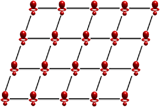
Figure 1: (color online). A two dimensional view of a crystal made of identical atoms prepared in exactly the same quantum superposition and with identical phase.

We assume the sub-units of the crystal to be noninteracting. The electronic states in Eq. (III.3) represent the state of the entire crystal, which factorizes into the electronic states of the individual sub-units. Due to the periodic structure of the crystal, the first term in Eq. (III.3) provides a coherent scattering signal giving rise to Bragg reflections. According to the Laue condition, for a sufficiently large crystal, the lattice sum allows scattering only at momentum transfer $\mathbf{Q}$ that is equal to a reciprocal lattice vector. For the coherent scattering, the lattice sum is a coherent sum, because it is impossible to distinguish at which sub-unit the scattering occurred. Thus, the Bragg intensity of the coherent scattering signal scales with the square of the number of unit cells in the crystal. The second term in Eq. (III.3) describes an incoherent scattering signal, where at one lattice site an electronic transition from the wave packet to a state that is not part of the wave packet is induced. Therefore, the sum over final states in Eq. (III.3) involves a sum over the different lattice sites. Because the site where the wave packet was destroyed can be distinguished from the other sites, the corresponding contributions must be summed incoherently. Thus, the intensity of the incoherent signal scales only linearly with the number of unit cells in the crystal.

In conclusion, the TRXS signal is dominated by the coherent scattering signal for a sufficiently large crystal. In the case of TRXS from a crystal, the instantaneous electron density $\langle\Phi|\hat{n}(\mathbf{x},\tau_{d})|\Phi\rangle$ of the wave packet can be retrieved from the coherent scattering signal. Although for a short pulse the bandwidth is large, the coherent signal dominates in the case of sufficiently many unit cells. It is important to mention that in the case of scattering from a single electronic wave packet, as demonstrated in our previous work dixit2012 ; dixit2013jcp , the contribution from the incoherent scattering signal dominates over the contribution from the coherent scattering signal.

IV Conclusion

This work is devoted to a rigorous understanding of TRXS to image coherent electronic motion on an ultrafast timescale using ultrashort hard x-ray pulses. The role of the pulse duration and of the energy resolution of the scattering detector have been investigated for TRXS. For stationary targets, long probe pulses can be used and the theory reduces to non-resonant x-ray scattering (elastic and inelastic). To image electronic wave packets one has to use ultrashort x-ray pulses. It is found that TRXS encodes the generalized dynamic structure factor and not the instantaneous electron density of an electronic wave packet. We have analyzed the scattering signal for two limiting situations of the energy resolution of the scattering detector. In both situations, the probe pulse duration sets the time resolution for the electronic motion. In the case of no energy resolution the scattering signal depends on the wave packet dynamics through the pump-probe delay and one measures the energy-integrated DSF which encodes the time-dependent electron pair-correlation function of the wave packet. Therefore, TRXS with no energy resolution is of particular importance as it seems feasible with existing detector technology and offers to image time-dependent electron correlations in dynamical electron systems. In the case of high energy resolution (small $\Delta E$) the scattering signal contains additional fingerprints of dynamics induced by the scattering process that are faster than the probe duration. They can be probed in the energy domain by varying the position ($\tilde{\omega}_{\mathbf{k}_{d}}$) of the spectral window function. We have made the connection of our theory to the dynamical imaging of ultrafast dynamics by Abbamonte and co-workers. In this way we have shown that from energy resolved x-ray scattering one can recover the electron density propagator for time scales much faster than the probe pulse duration. Thus, the present theory can be regarded as a unified description of time-resolved ultrafast x-ray scattering. The response of the density perturbation for an electronic wave packet within the linear-response theory has been investigated. We showed that the linear density response due to the scattering event itself vanishes. A special and interesting situation has been considered for TRXS from a crystal, consisting of identical electronic wave packets with identical phase at each lattice point. The scattering signal of the crystal is shown to recover the instantaneous electron density of the wave packet in this case. We hope that our present analysis of TRXS on ultrafast timescales will help in planning and understanding future experiments.

Appendix A First-order correlation function for x rays

The first-order correlation function is defined as

$$G^{(1)}(\mathbf{x}_{1},t_{1};\mathbf{x}_{2},t_{2}) = \textrm{Tr}[\hat{\rho}^{X}_{in}\hat{E}^{(-)}(\mathbf{x}_{1},t_{1})\hat{E}^{(+)}(\mathbf{x}_{2},t_{2})]$$ (27)

$$= \langle E^{(-)}(\mathbf{x}_{1},t_{1})E^{(+)}(\mathbf{x}_{2},t_{2})\rangle,$$

where $\hat{\rho}^{X}_{in}$ is the initial density operator for the x rays and $\hat{E}^{(+)}(\hat{E}^{(-)})$ is the positive (negative) component of the electric field operator. In the classical limit, the pulsed electric field can be expressed as

$$E(\mathbf{x},t)=E_{0}~{}\textrm{cos}(\mathbf{k}_{in}\cdot\mathbf{x}-\omega_{in}[t-\tau_{d}])~{}g(\mathbf{k}_{in}\cdot\mathbf{x}-\omega_{in}[t-\tau_{d}]),$$ (28)

where $\mathbf{k}_{in}$ and $\omega_{in}$ are, respectively, the carrier wave vector and the frequency of the pulsed field. Here, we assume that the envelope function $g$ is Gaussian:

$$g(\mathbf{k}_{in}\cdot\mathbf{x}-\omega_{in}[t-\tau_{d}])=e^{-\frac{1}{2\sigma^{2}\omega^{2}_{in}}(\mathbf{k}_{in}\cdot\mathbf{x}-\omega_{in}[t-\tau_{d}])^{2}},$$ (29)

where $\tau_{d}$ is the time delay and $\sigma$ is related to the pulse duration as $\tau_{l}=\sqrt{8\ln 2}~{}\sigma$. The probe pulse is assumed to propagate along the $z$ direction. Therefore, by using the Eqs. (28) and (29), the key quantity for the first-order correlation function is expressed as

$$E^{(-)}(z_{1},t_{1})E^{(+)}(z_{2},t_{2}) = \frac{1}{4}|E_{0}|^{2}~{}e^{-\frac{1}{2\sigma^{2}}(\alpha^{2}z_{1}^{2}+[t_{1}-\tau_{d}]^{2}-2\alpha z_{1}[t_{1}-\tau_{d}])}e^{i(k_{in}z_{1}-\omega_{in}t_{1})}$$ (30)

$$\times e^{-\frac{1}{2\sigma^{2}}(\alpha^{2}z_{2}^{2}+[t_{2}-\tau_{d}]^{2}-2\alpha z_{2}[t_{2}-\tau_{d}])}e^{-i(k_{in}z_{2}-\omega_{in}t_{2})}.$$

At this point, it is important to analyze the spatial dependence in Eq. (30), i.e., under which conditions the spatially dependent terms can be ignored and all the electrons in the sample experience a spatially uniform pulse envelope.  The spatially dependent terms, $\textrm{exp}[-\alpha^{2}z^{2}/2\sigma^{2}]$ and $\textrm{exp}[\alpha zt/\sigma^{2}]$, can be approximated by unity if the condition $\alpha|z|\ll\tau_{l}$ is satisfied. Here, $\tau_{l}$ is the pulse duration and $1/\alpha$ is the speed of light. Let us consider the situation considered in our previous works dixit2012 ; dixit2013jcp , where a 1-fs pulse duration has been used. Therefore, for the given value of $\tau_{l}$, $|z|\ll\tau_{l}/\alpha\simeq 300$  nanometers. Hence, for a sample size of tens of nanometers (or smaller) exposed to a few-fs hard x-ray pulse, the spatial dependence of the envelope of the incident pulse can be ignored. Note that we assume the object size to be small in comparison to the transverse size of the x-ray beam. Therefore, the first-order correlation function for x rays can be written as

$$G^{(1)}(\mathbf{x}_{1},t_{1};\mathbf{x}_{2},t_{2})=2\pi\alpha I(\tau)C(\delta)e^{-i\omega_{in}\delta}e^{i\mathbf{k}_{in}\cdot(\mathbf{x}-\mathbf{x}^{\prime})},$$ (31)

where $\tau=\frac{t_{1}+t_{2}}{2}$, $\delta=t_{2}-t_{1}$, and $C(\delta)=e^{-2\ln{2}\;\delta^{2}/\tau_{l}^{2}}$. Observe that the function $C(\delta)$ and thus the first-order correlation function vanish for time differences $\delta$ much larger than the pulse duration. Therefore, the function $C(\delta)$ describes the temporal coherence properties of the x rays.

Appendix B Density perturbation for an electronic wave packet within linear response theory

The physical density response can be written as

$$\delta{n}(\mathbf{x},t)=\textrm{Tr}[\hat{n}(\mathbf{x},t)\delta\hat{\rho}(t)],$$ (32)

where $\delta\hat{\rho}(t)$ is the change in the density operator within linear-response theory and can be written as

$$\delta\hat{\rho}(t)=\hat{\rho}^{(0,1)}(t)+\hat{\rho}^{(1,0)}(t),$$ (33)

with

$$\hat{\rho}^{(0,1)}(t)=\sum_{\{n\},\{\bar{n}\}}\rho^{X}_{\{n\},\{\bar{n}\}}|\Psi_{\{n\}}\rangle\langle\Psi_{\{\bar{n}\}}^{(1)},t|.$$ (34)

Here, $\rho^{X}_{\{n\},\{\bar{n}\}}$ represents the populations and coherences of all the occupied field modes of the incident radiation. Here, we have assumed that with the help of a pump pulse an electronic wave packet, $|\Phi\rangle$, is prepared and $|\Psi_{\{n\}}\rangle=|\Phi\rangle|\{n\}\rangle$ is a product state of electronic and photon states. The first order change of the state vector in the interaction picture can be written as

$$|\Psi^{(1)}_{\{n\}},t\rangle=(-i)\int_{-\infty}^{t}dt^{\prime}\hat{H}_{\textrm{int}}(t^{\prime})|\Psi_{\{n\}}\rangle.$$ (35)

On substituting the expressions from Eqs. (33) and  (34) in Eq. (32), the physical density-response can be expressed as

$$\delta{n}(\mathbf{x},t) = \textrm{Tr}[\hat{n}(\mathbf{x},t)(\hat{\rho}^{(0,1)}(t)+\hat{\rho}^{(1,0)}(t))]$$ (36)

$$= -i\sum_{\{n\},\{\bar{n}\}}\rho^{X}_{\{n\},\{\bar{n}\}}\int_{-\infty}^{t}dt^{\prime}\langle\Psi_{\{\bar{n}\}}|[\hat{n}(\mathbf{x},t),\hat{H}_{\textrm{int}}(t^{\prime})]|\Psi_{\{n\}}\rangle.$$

Now, on using the second term of $\hat{H}_{\textrm{int}}$ as shown in Eq. (1) ($\hat{\mathbf{A}}^{2}$ term), the above equation can be written as

$$\delta{n}(\mathbf{x},t)=(-i)\frac{\alpha^{2}}{2}\int_{-\infty}^{t}dt^{\prime}\int d^{3}x^{\prime}\textrm{Tr}[\hat{\rho}^{X}_{in}\hat{\mathbf{A}}^{2}(\mathbf{x}^{\prime},t^{\prime})]\langle\Phi|[\hat{n}(\mathbf{x},t),\hat{n}(\mathbf{x}^{\prime},t^{\prime})]|\Phi\rangle,$$ (37)

which can be expressed in the following known form as fetter1971

$$\delta{n}(\mathbf{x},t)=\int_{-\infty}^{t}dt^{\prime}\int d^{3}x^{\prime}\chi(\mathbf{x},\mathbf{x}^{\prime},t,t^{\prime})V(\mathbf{x}^{\prime},t^{\prime}).$$ (38)

On comparing Eq. (37) with Eq. (38), we can write the linear-response function at position $\mathbf{x}$ and time $t$ due to the external potential at position $\mathbf{x}^{\prime}$ and time $t^{\prime}$ as

$$\chi(\mathbf{x},\mathbf{x}^{\prime},t,t^{\prime})=-i~{}\langle\Phi|[\hat{n}(\mathbf{x},t),\hat{n}(\mathbf{x}^{\prime},t^{\prime})]|\Phi\rangle,$$ (39)

and the interaction potential as

$$V(\mathbf{x}^{\prime},t^{\prime})=\frac{\alpha^{2}}{2}\textrm{Tr}[\hat{\rho}^{X}_{in}\hat{\mathbf{A}}^{2}(\mathbf{x}^{\prime},t^{\prime})].$$ (40)

In the following, we will simplify $V(\mathbf{x}^{\prime},t^{\prime})$, which can be expressed in terms of the electric field operator as

$$V(\mathbf{x}^{\prime},t^{\prime}) = \frac{\alpha^{2}}{2\omega_{\mathbf{k}_{in}}^{2}}\textrm{Tr}[\hat{\rho}^{X}_{in}\hat{\mathbf{E}}^{2}(\mathbf{x}^{\prime},t^{\prime})]$$ (41)

$$= \frac{\alpha^{2}}{2\omega_{\mathbf{k}_{in}}^{2}}\left[\textrm{Tr}[\hat{\rho}_{in}^{X}\hat{\mathbf{E}}^{(-)}(\mathbf{x}^{\prime},t^{\prime})\hat{\mathbf{E}}^{(+)}(\mathbf{x}^{\prime},t^{\prime})]+\textrm{Tr}[\hat{\rho}_{in}^{X}\hat{\mathbf{E}}^{(+)}(\mathbf{x}^{\prime},t^{\prime})\hat{\mathbf{E}}^{(-)}(\mathbf{x}^{\prime},t^{\prime})]\right.$$

$$\left.+\textrm{Tr}[\hat{\rho}_{in}^{X}\hat{\mathbf{E}}^{(+)}(\mathbf{x}^{\prime},t^{\prime})\hat{\mathbf{E}}^{(+)}(\mathbf{x}^{\prime},t^{\prime})]+\textrm{Tr}[\hat{\rho}_{in}^{X}\hat{\mathbf{E}}^{(-)}(\mathbf{x}^{\prime},t^{\prime})\hat{\mathbf{E}}^{(-)}(\mathbf{x}^{\prime},t^{\prime})]\right].$$

On using the expressions for the pulsed electric field and envelope function [see Eqs. (28) and (29), respectively], and using a similar procedure as shown in appendix (A), the above equation can be simplified as

$$V(\mathbf{x}^{\prime},t^{\prime})=\frac{\alpha^{2}}{2\omega_{\mathbf{k}_{in}}^{2}}\left[\frac{1}{2}E_{0}g(\mathbf{k}_{in}\cdot\mathbf{x}^{\prime}-\omega_{\mathbf{k}_{in}}[t^{\prime}-\tau_{d}])\right]^{2}\left[2+e^{-2i(\mathbf{k}_{in}\cdot\mathbf{x}^{\prime}-\omega_{\mathbf{k}_{in}}t^{\prime})}+e^{2i(\mathbf{k}_{in}\cdot\mathbf{x}^{\prime}-\omega_{\mathbf{k}_{in}}t^{\prime})}\right].$$ (42)

Here, we assume that all the electrons in the sample experience a uniform pulse envelope and hence the spatial dependency of the envelope function can be ignored [see appendix (A)]. Therefore, Eq. (42) reduces to

$$V(\mathbf{x}^{\prime},t^{\prime})=\frac{\pi\alpha^{3}}{\omega_{\mathbf{k}_{in}}^{2}}I(t^{\prime})\left[2+e^{-2i(\mathbf{k}_{in}\cdot\mathbf{x}^{\prime}-\omega_{\mathbf{k}_{in}}t^{\prime})}+e^{2i(\mathbf{k}_{in}\cdot\mathbf{x}^{\prime}-\omega_{\mathbf{k}_{in}}t^{\prime})}\right].$$ (43)

Therefore, on substituting the expressions from Eqs. (42) and  (39), the density response can be written as

$$\delta{n}(\mathbf{x},t)=\frac{2\pi\alpha^{3}}{\omega_{\mathbf{k}_{in}}^{2}}\int_{-\infty}^{t}dt^{\prime}I(t^{\prime})\int d^{3}x^{\prime}\chi(\mathbf{x},\mathbf{x}^{\prime},t,t^{\prime})\left[1+\textrm{cos}[2(\mathbf{k}_{in}\cdot\mathbf{x}^{\prime}-\omega_{\mathbf{k}_{in}}t^{\prime})]\right].$$ (44)

The total density response can be decomposed into two parts as

$$\delta{n}(\mathbf{x},t)=\delta{n}_{1}(\mathbf{x},t)+\delta{n}_{2}(\mathbf{x},t),$$ (45)

where

$$\delta{n}_{1}(\mathbf{x},t)=\frac{2\pi\alpha^{3}}{\omega_{\mathbf{k}_{in}}^{2}}\int_{-\infty}^{t}dt^{\prime}I(t^{\prime})\int d^{3}x^{\prime}\chi(\mathbf{x},\mathbf{x}^{\prime},t,t^{\prime}),$$ (46)

and

$$\delta{n}_{2}(\mathbf{x},t)=\frac{2\pi\alpha^{3}}{\omega_{\mathbf{k}_{in}}^{2}}\int_{-\infty}^{t}dt^{\prime}I(t^{\prime})\int d^{3}x^{\prime}\chi(\mathbf{x},\mathbf{x}^{\prime},t,t^{\prime})\textrm{cos}[2(\mathbf{k}_{in}\cdot\mathbf{x}^{\prime}-\omega_{\mathbf{k}_{in}}t^{\prime})].$$ (47)

On performing the $\mathbf{x}^{\prime}$-dependent integral in Eq. (46), one finds that $\delta{n}_{1}(\mathbf{x},t)=0$. Thus, for perfectly stable (coherent) x rays, the density response for an electronic wave packet can be written as

$$\delta{n}(\mathbf{x},t)=\frac{2\pi\alpha^{3}}{\omega_{\mathbf{k}_{in}}^{2}}\int_{-\infty}^{t}dt^{\prime}I(t^{\prime})\int d^{3}x^{\prime}\chi(\mathbf{x},\mathbf{x}^{\prime},t,t^{\prime})\textrm{cos}[2(\mathbf{k}_{in}\cdot\mathbf{x}^{\prime}-\omega_{\mathbf{k}_{in}}t^{\prime})].$$ (48)

Appendix C Connection between linear-response function and dynamical structure factor

The retarded electron density propagator

$$\chi(\mathbf{x},\mathbf{x}^{\prime},t,t^{\prime})=-i\,\langle\Phi|[\hat{n}(\mathbf{x},t),\hat{n}(\mathbf{x}^{\prime},t^{\prime})]|\Phi\rangle\,\theta(t-t^{\prime}),$$ (49)

describes the propagation of disturbances in the electron density and characterizes the electronic system. The step function $\theta(t-t^{\prime})$ ensures causality. To connect the dynamical properties of the system with the temporal coherence of the probe pulse, we define the generalized propagator

$$\tilde{\chi}(\mathbf{x},\mathbf{x}^{\prime},t,t^{\prime})=-i\,C(t-t^{\prime})\,\langle\Phi|[\hat{n}(\mathbf{x},t),\hat{n}(\mathbf{x}^{\prime},t^{\prime})]|\Phi\rangle\,\theta(t-t^{\prime}),$$ (50)

where $C(t-t^{\prime})=\exp[{-2\ln{2}\;(t-t^{\prime})^{2}/\tau_{l}^{2}}]$ describes the temporal coherence of the x-ray pulse with pulse duration $\tau_{l}$, see Eq. (31). Observe that this propagator vanishes when $t-t^{\prime}$ is much larger than the pulse duration. As before, we image the system at a pump-probe delay time $\tau_{d}$ with a pulse duration short enough to freeze the wave packet. Thus, $|t-\tau_{d}|$ and $|t^{\prime}-\tau_{d}|$ of interest are small with respect to the wave packet motion and we can write the generalized propagator in terms of $\delta=t-t^{\prime}$ and $\tau_{d}$,

$$\tilde{\chi}(\mathbf{x},\mathbf{x}^{\prime},\delta,\tau_{d}) := \tilde{\chi}(\mathbf{x},\mathbf{x}^{\prime},t,t^{\prime})$$ (52)

$$= -i\;C(\delta)\,\theta(\delta)\sum_{f}\left[\langle\Phi|\hat{n}(\mathbf{x},\tau_{d})|\Psi_{f}\rangle\langle\Psi_{f}|\hat{n}(\mathbf{x}^{\prime},\tau_{d})|\Phi\rangle e^{i(\tilde{E}-E_{f})\delta}\right.$$

$$\left.-\langle\Phi|\hat{n}(\mathbf{x}^{\prime},\tau_{d})|\Psi_{f}\rangle\langle\Psi_{f}|\hat{n}(\mathbf{x},\tau_{d})|\Phi\rangle e^{i(E_{f}-\tilde{E})\delta}\right].$$

The Fourier transform with respect to $\mathbf{x},\mathbf{x}^{\prime}$ and $\delta$ is given by

$$\tilde{\chi}(\mathbf{Q},\mathbf{Q}^{\prime},\omega,\tau_{d}) =\iiint d\delta d^{3}x\,d^{3}x^{\prime}e^{i\omega\delta}e^{i\mathbf{Q}\cdot\mathbf{x}}\,e^{i\mathbf{Q}^{\prime}\cdot\mathbf{x}^{\prime}}\;\tilde{\chi}(\mathbf{x},\mathbf{x}^{\prime},\delta,\tau_{d})$$ (53)

$$=-i\sum_{f}\iint d^{3}x\,d^{3}x^{\prime}e^{i(\mathbf{Q}\cdot\mathbf{x}+\mathbf{Q}^{\prime}\cdot\mathbf{x}^{\prime})}\int d\delta\,C(\delta)\,\theta(\delta)$$

$$\quad\times\Big{[}e^{i(\omega+\tilde{E}-E_{f})\delta}\langle\Phi|\hat{n}(\mathbf{x},\tau_{d})|\Psi_{f}\rangle\langle\Psi_{f}|\hat{n}(\mathbf{x}^{\prime},\tau_{d})|\Phi\rangle$$

$$\quad-e^{i(\omega-\tilde{E}+E_{f})\delta}\langle\Phi|\hat{n}(\mathbf{x}^{\prime},\tau_{d})|\Psi_{f}\rangle\langle\Psi_{f}|\hat{n}(\mathbf{x},\tau_{d})|\Phi\rangle\Big{]}.$$ (54)

Now, one can easily determine the imaginary part of $\tilde{\chi}(\mathbf{Q},-\mathbf{Q},\omega,\tau_{d})$

$$\mathrm{Im}\big{[}\tilde{\chi}(\mathbf{Q},-\mathbf{Q},\omega,\tau_{d})\big{]} =-\pi\sum_{f}\frac{\tau_{l}}{\sqrt{8\pi\ln 2}}e^{-\frac{\tau_{l}}{8\ln 2}(\omega+\tilde{E}-E_{f})^{2}}\left|\int d^{3}x\,\langle\Psi_{f}|\hat{n}(\mathbf{x},\tau_{d})|\Phi\rangle e^{i\mathbf{Q}\cdot\mathbf{x}}\right|^{2}$$

$$\quad+\pi\sum_{f}\frac{\tau_{l}}{\sqrt{8\pi\ln 2}}e^{-\frac{\tau_{l}}{8\ln 2}(-\omega+\tilde{E}-E_{f})^{2}}\left|\int d^{3}x\,\langle\Psi_{f}|\hat{n}(\mathbf{x},\tau_{d})|\Phi\rangle e^{i\mathbf{Q}\cdot\mathbf{x}}\right|^{2}$$ (55)

$$=-\pi[\tilde{S}(\mathbf{Q},\omega,\tau_{d})-\tilde{S}(\mathbf{Q},-\omega,\tau_{d})].$$ (56)

This establishes the relation of the measured generalized DSF and the imaginary part of the generalized density propagator. Applying the four-step recipe by Abbamonte and coworkers abbamonte2004imaging ; abbamonte2010ultrafast one can reconstruct real-space information about $\tilde{\chi}$. From the definition of the generalized propagator, we see that for time propagation much shorter than the pulse duaration ( $\delta\ll\tau_{l}$) this gives information about the density propagator. Observe, that the generalized DSF only provides the diagonal terms, where $\mathbf{Q}^{\prime}=-\mathbf{Q}$. It was shown in Ref. abbamonte2009inhomogeneous that one recovers the full electron density propagator only for homogeneous systems, whereas for the case of an inhomogeneous system one obtains the averaged generalized propagator

$$\tilde{\chi}(\mathbf{x},\delta,\tau_{d})=\int d^{3}x^{\prime}\,\tilde{\chi}(\mathbf{x}+\mathbf{x}^{\prime},\mathbf{x}^{\prime},\delta,\tau_{d})\,,$$

averaged over all possible source locations $\mathbf{x}^{\prime}$.

References

• (1) H. Ihee, M. Lorenc, T. K. Kim, Q. Y. Kong, M. Cammarata, J. H. Lee, S. Bratos, and M. Wulff, Science 309, 1223 (2005).
• (2) H. N. Chapman, P. Fromme, A. Barty, T. A. White, R. A. Kirian, A. Aquila, M. S. Hunter, J. Schulz, D. P. DePonte, U. Weierstall, R. B. Doak, F. R. N. C. Maia, A. V. Martin, I. Schlichting, L. Lomb, N. Coppola, R. L. Shoeman, S. W. Epp, R. Hartmann, D. Rolles, A. Rudenko, L. Foucar, N. Kimmel, G. Weidenspointner, P. Holl, M. Liang, M. Barthelmess, C. Caleman, S. Boutet, M. J. Bogan, J. Krzywinski, C. Bostedt, S. Bajt, L. Gumprecht, B. Rudek, B. Erk, C. Schmidt, A. H mke, C. Reich, D. Pietschner, L. Str der, G. Hauser, H. Gorke, J. Ullrich, S. Herrmann, G. Schaller, F. Schopper, H. Soltau, K. U. K hnel, M. Messerschmidt, J. D. Bozek, S. P. Hau-Riege, M. Frank, C. Y. Hampton, R. G. Sierra, D. Starodub, G. J. Williams, J. Hajdu, N. Timneanu, M. M. Seibert, J. Andreasson, A. Rocker, O. J nsson, M. Svenda, S. Stern, K. Nass, R. Andritschke, C. D. Schroeter, F. Krasniqi, M. Bott, K. E. Schmidt, X. Wang, I. Grotjohann, J. M. Holton, T. R. M. Barends, R. Neutze, S. Marchesini, R. Fromme, S. Schorb, D. Rupp, M. Adolph, T. Gorkhover, I. Andersson, H. Hirsemann, G. Potdevin, H. Graafsma, B. Nilsson, and J. C. H. Spence, Nature 470, 73 (2011).
• (3) M. M. Seibert, T. Ekeberg, F. R. N. C. Maia, M. Svenda, J. Andreasson, O. Jonsson, D. Odic, B. Iwan, A. Rocker, D. Westphal, M. Hantke, D. P. DePonte, A. Barty, J. Schulz, L. Gumprecht, N. Coppola, A. Aquila, M. N. Liang, T. A. White, A. Martin, C. Caleman, S. Stern, C. Abergel, V. Seltzer, J. M. Claverie, C. Bostedt, J. D. Bozek, S. Boutet, A. A. Miahnahri, M. Messerschmidt, J. Krzywinski, G. Williams, K. O. Hodgson, M. J. Bogan, C. Y. Hampton, R. G. Sierra, D. Starodub, I. Andersson, S. Bajt, M. Barthelmess, J. C. H. Spence, P. Fromme, U. Weierstall, R. Kirian, M. Hunter, R. B. Doak, S. Marchesini, S. P. Hau-Riege, M. Frank, R. L. Shoeman, L. Lomb, S. W. Epp, R. Hartmann, D. Rolles, A. Rudenko, C. Schmidt, L. Foucar, N. Kimmel, P. Holl, B. Rudek, B. Erk, A. Homke, C. Reich, D. Pietschner, G. Weidenspointner, L. Struder, G. Hauser, H. Gorke, J. Ullrich, I. Schlichting, S. Herrmann, G. Schaller, F. Schopper, H. Soltau, K. U. Kuhnel, R. Andritschke, C. D. Schroter, F. Krasniqi, M. Bott, S. Schorb, D. Rupp, M. Adolph, T. Gorkhover, H. Hirsemann, G. Potdevin, H. Graafsma, B. Nilsson, H. N. Chapman, and J. Hajdu, Nature 470, 78 (2011).
• (4) H. N. Chapman and K. A. Nugent, Nature Photonics 4, 833 (2010).
• (5) B. Abbey, L. W. Whitehead, H. M. Quiney, D. J. Vine, G. A. Cadenazzi, C. A. Henderson, K. A. Nugent, E. Balaur, C. T. Putkunz, A. G. Peele, G. J. Williams, and I. McNulty, Nature Photonics 5, 420 (2011).
• (6) J. Miao, P. Charalambous, J. Kirz, and D. Sayre, Nature 400, 342 (1999).
• (7) J. M. Zuo, I. Vartanyants, M. Gao, R. Zhang, and L. A. Nagahara, Science 300, 1419 (2003).
• (8) P. Emma, R. Akre, J. Arthur, R. Bionta, C. Bostedt, J. Bozek, A. Brachmann, P. Bucksbaum, R. Coffee, F. J. Decker, Y. Ding, D. Dowell, S. Edstrom, A. Fisher, J. Frisch, S. Gilevich, J. Hastings, G. Hays, P. Hering, Z. Huang, R. Iverson, H. Loos, M. Messerschmidt, A. Miahnahri, S. Moeller, H. D. Nuhn, G. Pile, D. Ratner, J. Rzepiela, D. Schultz, T. Smith, P. Stefan, H. Tompkins, J. Turner, J. Welch, W. White, J. Wu, G. Yocky, and J. Galayda, Nature Photonics 4, 641 (2010).
• (9) T. Ishikawa, H. Aoyagi, T. Asaka, Y. Asano, N. Azumi, T. Bizen, H. Ego, K. Fukami, T. Fukui, Y. Furukawa, S. Goto, H. Hanaki, T. Hara, T. Hasegawa, T. Hatsui, A. Higashiya, T. Hirono, N. Hosoda, M. Ishii, T. Inagaki, Y. Inubushi, T. Itoga, Y. Joti, M. Kago, T. Kameshima, H. Kimura, Y. Kirihara, A. Kiyomichi, T. Kobayashi, C. Kondo, T. Kudo, H. Maesaka, X. M. Marechal, S. Masuda, T.and Matsubara, T. Matsumoto, T. Matsushita, S. Matsui, M. Nagasono, N. Nariyama, H. Ohashi, T. Ohata, T. Ohshima, S. Ono, Y. Otake, C. Saji, T. Sakurai, T. Sato, K. Sawada, T. Seike, K. Shirasawa, T. Sugimoto, S. Suzuki, S. Takahashi, H. Takebe, K. Takeshita, K. Tamasaku, H. Tanaka, R. Tanaka, T. Tanaka, T. Togashi, K. Togawa, A. Tokuhisa, H. Tomizawa, K. Tono, S. K. Wu, M. Yabashi, M. Yamaga, A. Yamashita, K. Yanagida, C. Zhang, T. Shintake, H. Kitamura, and N. Kumagai, Nature Photonics 6, 540 (2012).
• (10) F. Krausz and M. Ivanov, Rev. Mod. Phys. 81, 163 (2009).
• (11) P. H. Bucksbaum, Science 317, 766 (2007).
• (12) P. B. Corkum and F. Krausz, Nature Physics 3, 381 (2007).
• (13) J. Breidbach and L. S. Cederbaum, J. Chem. Phys. 118, 3983 (2003).
• (14) A. I. Kuleff, J. Breidbach, and L. S. Cederbaum, J. Chem. Phys. 123, 044111 (2005).
• (15) F. Remacle and R. D. Levine, Proc. Natl. Acad. Sci. U.S.A 103, 6793 (2006).
• (16) A. D. Dutoi and L. S. Cederbaum, J. Phys. Chem. Lett. 2, 2300 (2011).
• (17) A. J. Benedick, J. G. Fujimoto, and F. X. Kärtner, Nature Photonics 6, 97 (2012).
• (18) P. Emma, K. Bane, M. Cornacchia, Z. Huang, H. Schlarb, G. Stupakov, and D. Walz, Phys. Rev. Lett. 92, 74801 (2004).
• (19) A. A. Zholents and W. M. Fawley, Phys. Rev. Lett. 92, 224801 (2004).
• (20) T. Tanaka, Phys. Rev. Lett. 110, 084801 (2013).
• (21) S. Kumar, H. S. Kang, and D. E. Kim, Applied Sciences 3, 251 (2013).
• (22) G. Dixit, O. Vendrell, and R. Santra, Proc. Natl. Acad. Sci. U.S.A. 109, 11636 (2012).
• (23) G. Dixit and R. Santra, J. Chem. Phys. 138, 134311 (2013).
• (24) G. Dixit, J. M. Slowik, and R. Santra, Phys. Rev. Lett. 110, 137403 (2013).
• (25) P. Abbamonte, K. D. Finkelstein, M. D. Collins, and S. M. Gruner, Phys. Rev. Lett. 92, 237401 (2004).
• (26) P. Abbamonte, T. Graber, J. P. Reed, S. Smadici, C. L. Yeh, A. Shukla, J. P. Rueff, and W. Ku, Proc. Natl. Acad. Sci. U.S.A. 105, 12159 (2008).
• (27) P. Abbamonte, G. C. L. Wong, D. G. Cahill, J. P. Reed, R. H. Coridan, N. W. Schmidt, G. H. Lai, Y. I. Joe, and D. Casa, Advanced Materials 22, 1141 (2010).
• (28) P. Abbamonte, J. P. Reed, Y. I. Joe, Y. Gan, and D. Casa, Phys. Rev. B 80, 054302 (2009).
• (29) Y. Gan, A. Kogar, and P. Abbamonte, Chem. Phys. 414, 160 (2013).
• (30) D. P. Craig and T. Thirunamachandran, Molecular Quantum Electrodynamics, Academic Press, London, 1984.
• (31) M. W. Haverkort, A. Tanaka, L. H. Tjeng, and G. A. Sawatzky, Phys. Rev. Lett. 99, 257401 (2007).
• (32) R. Loudon, The Quantum Theory of Light, Oxford University Press, Oxford, 1983.
• (33) R. J. Glauber, Phys. Rev. 130, 2529 (1963).
• (34) N. E. Henriksen and K. B. Moller, J. Phys. Chem. B 112, 558 (2008).
• (35) S. Tanaka, V. Chernyak, and S. Mukamel, Phys. Rev. A 63, 63405 (2001).
• (36) W. Schülke, Electron dynamics by inelastic X-ray scattering, Oxford University Press Oxford, UK, 2007.
• (37) L. Van Hove, Phys. Rev. 95, 249 (1954).
• (38) C. Petrillo and F. Sacchetti, Phys. Rev. B 51, 4755 (1995).
• (39) W. Schülke, J. R. Schmitz, H. Schulte-Schrepping and A. Kaprolat Phys. Rev. B 52, 11721 (1995).
• (40) N. Watanabe, H. Hayashi, Y. Udagawa, S. Ten-no and S. Iwata J. Chem. Phys. 108, 4545 (1998).
• (41) A. L. Fetter and J. D. Walecka, Quantum Theory of Many-Particle Systems, McGraw-Hill, Boston, 1971.