Hopf Bifurcation in a Gene Regulatory Network Model:
Molecular Movement Causes Oscillations

Mark Chaplainaa\,{}^{\mathrm{a}}, Mariya Ptashnykaa\,{}^{\mathrm{a}} and Marc Sturrockbb\,{}^{\mathrm{b}}
a Division of Mathematics, University of Dundee, Dundee DD1 4HN, Scotland, UK
bMathematical Biosciences Institute, Ohio State University, 377 Jennings Hall,
1735 Neil Avenue, Columbus, OH, USA
Abstract

Gene regulatory networks, i.e. DNA segments in a cell which interact with each other indirectly through their RNA and protein products, lie at the heart of many important intracellular signal transduction processes. In this paper we analyse a mathematical model of a canonical gene regulatory network consisting of a single negative feedback loop between a protein and its mRNA (e.g. the Hes1 transcription factor system). The model consists of two partial differential equations describing the spatio-temporal interactions between the protein and its mRNA in a 1-dimensional domain. Such intracellular negative feedback systems are known to exhibit oscillatory behaviour and this is the case for our model, shown initially via computational simulations. In order to investigate this behaviour more deeply, we next solve our system using Greenโ€™s functions and then undertake a linearized stability analysis of the steady states of the model. Our results show that the diffusion coefficient of the protein/mRNA acts as a bifurcation parameter and gives rise to a Hopf bifurcation. This shows that the spatial movement of the mRNA and protein molecules alone is sufficient to cause the oscillations. This has implications for transcription factors such as p53, NF-ฮบ๐œ…\kappaB and heat shock proteins which are involved in regulating important cellular processes such as inflammation, meiosis, apoptosis and the heat shock response, and are linked to diseases such as arthritis and cancer.

1 Introduction

A gene regulatory network (GRN) can be defined as a collection of DNA segments in a cell which interact with each other indirectly through their RNA and protein products. GRNs lie at the heart of intracellular signal transduction and indirectly control many important cellular functions. A key component of GRNs is a class of proteins called transcription factors. In response to various biological signals, transcription factors change the transcription rate of genes, allowing cells to produce the proteins they need at the appropriate times and in the appropriate quantities. It is now well stablished that GRNs contain a small set of recurring regulation patterns, commonly referred to as network motifs [48], which can be thought of as recurring circuits of interactions from which complex GRNs are built. A GRN is said to contain a negative feedback loop if a gene product inhibits its own production either directly or indirectly. Negative feedback loops are commonly found in diverse biological processes including inflammation, meiosis, apoptosis and the heat shock response [1, 11, 39], and are known to exhibit oscillations in mRNA and protein levels [14, 36, 52].

Mathematical modelling of GRNs goes back to the work of Goodwin [18], where an initial system of two ordinary differential equations (ODEs) was used to model a self-repressing gene. In the final part of the paper a system of 3 ODEs was shown to produce limit cycle behaviour. This work was continued by Griffith [20] who demonstrated that the introduction of the third species was necessary for the oscillatory dynamics. An analysis of theoretical chemical systems whereby two chemicals produced at distinct spatial locations (heterogeneous catalysis) diffused and reacted together was carried out by Glass and co-workers [16, 58]. Their results showed that the number and stability of the steady states of the system changed depending on the distance between the two catalytic sites. The authors concluded that โ€œThese examples indicate that geometrical considerations must be explicitly considered when analyzing the dynamics of highly structured (e.g., biological) systems.โ€ [58]. Mahaffy and co-workers [5, 42, 43] developed this work further by considering an explicitly spatial model and also time delays accounting for the processes of transcription (production of mRNA) and translation (production of proteins). Tiana et al. [63] proposed that introducing delays to ODE models of negative feedback loops could produce sustained oscillatory dynamics and Jensen et al. [30] found that the invocation of an unknown third species (as Griffith had done [20]) could be avoided by the introduction of delay terms to a model of the Hes1 GRN (the justification being to account for the processes of transcription and translation). The Hes1 system is a simple example of a GRN which possesses a single negative feedback loop and benefits from having been the subject of numerous biological experiments [26, 31, 35, 36, 37]. A delay differential equation (DDE) model of the Hes1 GRN has also been studied by Monk and co-workers [49, 50]. More recently a 2-dimensional spatio-temporal model of the Hes1 GRN considering diffusion of the protein and mRNA was developed by Sturrock et al. [61] and then later extended to account for directed transport via microtublues [62].

A key feature of all mathematical models of the Hes1 GRN (and other negative feedback systems) is the existence of oscillatory solutions characterised by a Hopf bifurcation. In the Hopf, or Poincarรฉ-Andronov-Hopf bifurcation (first described by Hopf [27]), a steady state changes stability as two complex conjugate eigenvalues of the linearization cross the imaginary axis and a family of periodic orbits bifurcates from the steady state. Many studies are devoted to the existence and stability of Hopf bifurcations in ordinary and partial differential equations [6, 24, 34, 33, 38, 44]. The question of the existence of global Hopf bifurcation for nonlinear parabolic equations has also been considered [12, 13, 29]. There are many results concerning the stability of constant (i.e. spatially homogeneous) steady states and the existence of periodic solutions bifurcating from such constant steady states. There are some results on the stability of spike-solutions and the existence of Hopf bifurcations in the shadow Gierer-Meinhardt model [9, 53, 66, 65], as well as on the stability of spiky solutions in a reaction-diffusion system with four morphogens [68] and of cluster solutions for large reaction-diffusion systems [67]. In the analysis of the stability and Hopf bifurcations in systems with spike-solutions as stationary solutions, the properties of the corresponding nonlocal eigenvalue problem were used. Perturbation theory has been applied to analyse the stability of non-constant steady-states for a system of nonlinear reaction-diffusion equations coupled with ordinary differential equations [17]. In considering the relation between the spectrum of a linearised operator for singularly perturbed predator-prey-type equations with diffusion and the limit operator as the perturbation parameter tends to zero, Dancer [7] analysed the stability of strictly positive stationary solutions and the existence of Hopf bifurcations.

In this paper we analyse a mathematical model of the Hes1 transcription factor - a canonical GRN consisting of a single negative feedback loop between the Hes1 protein and its mRNA. The format of this paper is as follows. In the next section we present our mathematical model derived from that first formulated by Sturrock et al. [61]. First we demonstrate the existence of oscillatory solutions numerically, indicating the existence of Hopf bifurcations. Next, applying linearised stability analysis, we study the stability of a (spatially inhomogeneous) steady state of the model and prove the existence of a Hopf bifurcation. The main difficulty of the analysis is that the steady state of the model is not constant. In a similar manner to Dancer [7] we show the existence of a Hopf bifurcation by considering a limit problem associated with the original model. The method of collective compactness [2, 7] is applied to relate the spectrum of the limit operator to the spectrum of the original operator. To show the stability of periodic solutions and to determine the type of Hopf bifurcation, we use a weakly nonlinear analysis, see, for example, Matkowski [45], and normal form theory, see, for example, Hassard, Haragus [23, 24]. The techniques of weakly nonlinear analysis [10, 8, 40, 56] and normal form theory [23, 24], are widely used to study the nonlinear behaviour of solutions near bifurcation points.

2 The Mathematical Model of the Hes1 Gene Regulatory Network

The basic model of a self-repressing gene [50] describing the temporal dynamics of hes1 mRNA concentration, mโ€‹(t)๐‘š๐‘กm(t), and Hes1 protein concentration, pโ€‹(t)๐‘๐‘กp(t), takes the general form:

โˆ‚mโˆ‚t๐‘š๐‘ก\displaystyle\frac{\partial m}{\partial t} =\displaystyle= ฮฑmโ€‹fโ€‹(p)โˆ’ฮผmโ€‹m,subscript๐›ผ๐‘š๐‘“๐‘subscript๐œ‡๐‘š๐‘š\displaystyle\alpha_{m}f(p)-\mu_{m}m, (1)
โˆ‚pโˆ‚t๐‘๐‘ก\displaystyle\frac{\partial p}{\partial t} =\displaystyle= ฮฑpโ€‹mโˆ’ฮผpโ€‹p,subscript๐›ผ๐‘๐‘šsubscript๐œ‡๐‘๐‘\displaystyle\alpha_{p}m-\mu_{p}p, (2)

for positive constants ฮฑm,ฮฑp,ฮผm,ฮผpsubscript๐›ผ๐‘šsubscript๐›ผ๐‘subscript๐œ‡๐‘šsubscript๐œ‡๐‘\alpha_{m},\alpha_{p},\mu_{m},\mu_{p} and some function fโ€‹(p)๐‘“๐‘f(p) modelling the suppression of mRNA production by the protein. It can be shown using Bendixsonโ€™s Negative Criterion (cf. Verhulst [64], Theorem 4.1) that, irrespective of the function fโ€‹(p)๐‘“๐‘f(p) (e.g. a Hill function), there are no periodic solutions of the above system. In order to account for the experimentally observed oscillations in both mRNA and protein concentration levels [26], a discrete delay has often been introduced into such models being justified as taking into account the time taken to produce mRNA (transcription) and produce protein (translation) [50]. Applying a discrete delay ฯ„๐œ\tau to (1), (2), a delay differential equation model is obtained of the form:

โˆ‚mโˆ‚t๐‘š๐‘ก\displaystyle\frac{\partial m}{\partial t} =\displaystyle= ฮฑmโ€‹fโ€‹(pโˆ’ฯ„)โˆ’ฮผmโ€‹m,subscript๐›ผ๐‘š๐‘“๐‘๐œsubscript๐œ‡๐‘š๐‘š\displaystyle\alpha_{m}f(p-\tau)-\mu_{m}m, (3)
โˆ‚pโˆ‚t๐‘๐‘ก\displaystyle\frac{\partial p}{\partial t} =\displaystyle= ฮฑpโ€‹mโˆ’ฮผpโ€‹p.subscript๐›ผ๐‘๐‘šsubscript๐œ‡๐‘๐‘\displaystyle\alpha_{p}m-\mu_{p}p. (4)

Such a system is observed to exhibit oscillations for a suitable value of the delay parameter ฯ„๐œ\tau representing the sum of the transcriptional and translational time delays. This delay differential equation approach has also been used to model other feedback systems involving transcription factors such as p53 [3, 15, 63] and NF-ฮบ๐œ…\kappaB [52]. Other papers have used a distributed delay to model this effect[19], which in fact is equivalent to the original three ODE model of a self-repressing gene proposed by Goodwin [18] and Griffith [20].

Here we study an explicitly spatial model of the Hes1 GRN originally formulated by Sturrock et al. [61, 62] and investigate the role that spatial movement of the molecules may play in causing the oscillations in concentration levels. The model consists of a system of coupled nonlinear partial differential equations describing the temporal and spatial dynamics of the concentration of hes1 mRNA, mโ€‹(x,t)๐‘š๐‘ฅ๐‘กm(x,t), and Hes1 protein, pโ€‹(x,t)๐‘๐‘ฅ๐‘กp(x,t), and accounts for the processes of transcription (mRNA production) and translation (protein production). Transcription is assumed to occur in a small region of the domain representing the gene site. Both mRNA and protein also diffuse and undergo linear decay. The non-dimensionalised model is given as:

โˆ‚mโˆ‚t=Dโ€‹โˆ‚2mโˆ‚x2+ฮฑmโ€‹fโ€‹(p)โ€‹ฮดxMฮตโ€‹(x)โˆ’ฮผโ€‹mย inย โ€‹(0,T)ร—(0,1),โˆ‚pโˆ‚t=Dโ€‹โˆ‚2pโˆ‚x2+ฮฑpโ€‹gโ€‹(x)โ€‹mโˆ’ฮผโ€‹pย inย โ€‹(0,T)ร—(0,1),โˆ‚mโ€‹(t,0)โˆ‚x=โˆ‚mโ€‹(t,1)โˆ‚x=0,โˆ‚pโ€‹(t,0)โˆ‚x=โˆ‚pโ€‹(t,1)โˆ‚x=0ย inย โ€‹(0,T),mโ€‹(0,x)=m0โ€‹(x),pโ€‹(0,x)=p0โ€‹(x)ย inย โ€‹(0,1),missing-subexpression๐‘š๐‘ก๐ทsuperscript2๐‘šsuperscript๐‘ฅ2subscript๐›ผ๐‘š๐‘“๐‘subscriptsuperscript๐›ฟ๐œ€subscript๐‘ฅ๐‘€๐‘ฅ๐œ‡๐‘šย inย 0๐‘‡01missing-subexpression๐‘๐‘ก๐ทsuperscript2๐‘superscript๐‘ฅ2subscript๐›ผ๐‘๐‘”๐‘ฅ๐‘š๐œ‡๐‘ย inย 0๐‘‡01missing-subexpressionformulae-sequence๐‘š๐‘ก0๐‘ฅ๐‘š๐‘ก1๐‘ฅ0๐‘๐‘ก0๐‘ฅ๐‘๐‘ก1๐‘ฅ0ย inย 0๐‘‡missing-subexpressionformulae-sequence๐‘š0๐‘ฅsubscript๐‘š0๐‘ฅ๐‘0๐‘ฅsubscript๐‘0๐‘ฅย inย 01\displaystyle\begin{aligned} &\frac{\partial m}{\partial t}=D\frac{\partial^{2}m}{\partial x^{2}}+\alpha_{m}\,f(p)\delta^{\varepsilon}_{x_{M}}(x)-\mu\,m\quad&\text{ in }(0,T)\times(0,1),\\ &\frac{\partial p}{\partial t}=D\frac{\partial^{2}p}{\partial x^{2}}+\alpha_{p}\,g(x)\,m-\mu\,p\quad&\text{ in }(0,T)\times(0,1),\\ &\frac{\partial m(t,0)}{\partial x}=\frac{\partial m(t,1)}{\partial x}=0,\quad\frac{\partial p(t,0)}{\partial x}=\frac{\partial p(t,1)}{\partial x}=0\quad&\text{ in }(0,T),\\ &m(0,x)=m_{0}(x),\quad p(0,x)=p_{0}(x)\quad&\text{ in }(0,1),\end{aligned} (5)

where D๐ทD, ฮฑmsubscript๐›ผ๐‘š\alpha_{m}, ฮฑpsubscript๐›ผ๐‘\alpha_{p} and ฮผ๐œ‡\mu are positive constants (the diffusion coefficient, transcription rate, translation rate and decay rate respectively). Here l๐‘™l denotes the position of the nuclear membrane and therefore the domain is partitioned into two distinct regions, (0,l)0๐‘™(0,l) the cell nucleus and (l,1)๐‘™1(l,1) the cell cytoplasm, for some lโˆˆ(0,1)๐‘™01l\in(0,1). The point xMโˆˆ(0,l)subscript๐‘ฅ๐‘€0๐‘™x_{M}\in(0,l) is the position of the centre of the gene site and by ฮดxMฮตsubscriptsuperscript๐›ฟ๐œ€subscript๐‘ฅ๐‘€\delta^{\varepsilon}_{x_{M}} we denote the Dirac approximation of the ฮด๐›ฟ\delta-distribution located at xMsubscript๐‘ฅ๐‘€x_{M}, with ฮต>0๐œ€0\varepsilon>0 a small parameter and ฮดxMฮตsubscriptsuperscript๐›ฟ๐œ€subscript๐‘ฅ๐‘€\delta^{\varepsilon}_{x_{M}} has compact support.

The nonlinear reaction term f:โ„โ†’โ„:๐‘“โ†’โ„โ„f:\mathbb{R}\to\mathbb{R} is a Hill function fโ€‹(p)=1/(1+ph)๐‘“๐‘11superscript๐‘โ„Žf(p)={1}/{(1+p^{h})}, with hโ‰ฅ1โ„Ž1h\geq 1, modelling the suppression of mRNA production by the protein (negative feedback). The function g๐‘”g is a step function given by

gโ€‹(x)={0,ifโ€‹x<l,1,ifโ€‹xโ‰ฅl,๐‘”๐‘ฅcases0if๐‘ฅ๐‘™missing-subexpressionmissing-subexpression1if๐‘ฅ๐‘™g(x)=\left\{\begin{array}[]{ll}0,&\mbox{if}\,\,x<l\;,\\ \\ 1,&\mbox{if}\,\,x\geq l\;,\\ \end{array}\right.

since the process of translation only occurs in the cytoplasm. A schematic diagram of the domain is given in Figure 1.

Refer to caption
Figure 1: Schematic diagram of the 1-dimensional spatial domain for the system (5), showing the spatial location of the gene site xMsubscript๐‘ฅ๐‘€x_{M} and the nuclear membrane l๐‘™l. The cell nucleus is shown in blue, while the cell cytoplasm is shown in green.

First we demonstrate existence and uniqueness of solutions to (5).

Theorem 2.1.

For ฮต>0๐œ€0\varepsilon>0 and nonnegative initial data m0,p0โˆˆH2โ€‹(0,1)subscript๐‘š0subscript๐‘0superscript๐ป201m_{0},p_{0}\in H^{2}(0,1), there exists a unique nonnegative global solution m,pโˆˆCโ€‹([0,โˆž);H2โ€‹(0,1))๐‘š๐‘๐ถ0superscript๐ป201m,p\in C([0,\infty);H^{2}(0,1)), โˆ‚tm,โˆ‚tpโˆˆL2โ€‹((0,T)ร—(0,1))subscript๐‘ก๐‘šsubscript๐‘ก๐‘superscript๐ฟ20๐‘‡01\partial_{t}m,\partial_{t}p\in L^{2}((0,T)\times(0,1)), and m,pโˆˆC(ฮณ+1)/2,ฮณ+1โ€‹([0,T]ร—[0,1])๐‘š๐‘superscript๐ถ๐›พ12๐›พ10๐‘‡01m,p\in C^{(\gamma+1)/2,\gamma+1}([0,T]\times[0,1]), for some ฮณ>0๐›พ0\gamma>0 and any T>0๐‘‡0T>0, of the problem (5) satisfying

โ€–mโ€–Lโˆžโ€‹(0,T;H1โ€‹(0,1))+โ€–pโ€–Lโˆžโ€‹(0,T;H1โ€‹(0,1))โ‰คC,โ€–โˆ‚tmโ€–L2โ€‹((0,T)ร—(0,1))+โ€–โˆ‚tpโ€–L2โ€‹(0,T;H1โ€‹(0,1))+โ€–โˆ‚x2pโ€–L2โ€‹((0,T)ร—(0,1))โ‰คC,subscriptnorm๐‘šsuperscript๐ฟ0๐‘‡superscript๐ป101subscriptnorm๐‘superscript๐ฟ0๐‘‡superscript๐ป101๐ถsubscriptnormsubscript๐‘ก๐‘šsuperscript๐ฟ20๐‘‡01subscriptnormsubscript๐‘ก๐‘superscript๐ฟ20๐‘‡superscript๐ป101subscriptnormsuperscriptsubscript๐‘ฅ2๐‘superscript๐ฟ20๐‘‡01๐ถ\displaystyle\begin{aligned} \|m\|_{L^{\infty}(0,T;H^{1}(0,1))}+\|p\|_{L^{\infty}(0,T;H^{1}(0,1))}\leq C,\\ \|\partial_{t}m\|_{L^{2}((0,T)\times(0,1))}+\|\partial_{t}p\|_{L^{2}(0,T;H^{1}(0,1))}+\|\partial_{x}^{2}p\|_{L^{2}((0,T)\times(0,1))}\leq C,\end{aligned} (6)

for any Tโˆˆ(0,โˆž)๐‘‡0T\in(0,\infty) with the constant C๐ถC independent of ฮต๐œ€\varepsilon.

Proof.

Since fโ€‹(p)๐‘“๐‘f(p) is Lipschitz continuous for pโ‰ฅโˆ’ฮธ๐‘๐œƒp\geq-\theta, with some 0<ฮธ<10๐œƒ10<\theta<1, we have that for nonnegative initial data m0subscript๐‘š0m_{0}, p0subscript๐‘0p_{0} the existence and uniqueness of a solution of the problem (5) in (0,T0)ร—(0,1)0subscript๐‘‡001(0,T_{0})\times(0,1), for some T0>0subscript๐‘‡00T_{0}>0, follows directly from the existence and the regularity theory for systems of parabolic equations, see e.g. Henry [25], Lieberman [41]. Using the definition of the Dirac sequence, for Fmโ€‹(m,p)=ฮฑmโ€‹fโ€‹(p)โ€‹ฮดxMฮตโ€‹(x)โˆ’ฮผโ€‹msubscript๐น๐‘š๐‘š๐‘subscript๐›ผ๐‘š๐‘“๐‘subscriptsuperscript๐›ฟ๐œ€subscript๐‘ฅ๐‘€๐‘ฅ๐œ‡๐‘šF_{m}(m,p)=\alpha_{m}\,f(p)\delta^{\varepsilon}_{x_{M}}(x)-\mu\,m and Fpโ€‹(m,p)=ฮฑpโ€‹gโ€‹(x)โ€‹mโˆ’ฮผโ€‹p,subscript๐น๐‘๐‘š๐‘subscript๐›ผ๐‘๐‘”๐‘ฅ๐‘š๐œ‡๐‘F_{p}(m,p)=\alpha_{p}\,g(x)\,m-\mu\,p, we have

Fm|m=0โ‰ฅ0ย forย โ€‹pโ‰ฅ0,formulae-sequenceevaluated-atsubscript๐น๐‘š๐‘š00ย forย ๐‘0\displaystyle F_{m}|_{m=0}\geq 0\quad\text{ for }p\geq 0,\quad Fp|p=0โ‰ฅ0ย forย โ€‹mโ‰ฅ0,formulae-sequenceevaluated-atsubscript๐น๐‘๐‘00ย forย ๐‘š0\displaystyle F_{p}|_{p=0}\geq 0\quad\hskip 42.67912pt\text{ for }m\geq 0,
Fm|m=ฮฑm/(ฮผโ€‹ฮต)โ‰ค0ย forย โ€‹pโ‰ฅ0,formulae-sequenceevaluated-atsubscript๐น๐‘š๐‘šsubscript๐›ผ๐‘š๐œ‡๐œ€0ย forย ๐‘0\displaystyle F_{m}|_{m=\alpha_{m}/(\mu\varepsilon)}\leq 0\quad\text{ for }p\geq 0,\quad Fp|p=ฮฑmโ€‹ฮฑp/(ฮผ2โ€‹ฮต)โ‰ค0ย forย โ€‹mโ‰คฮฑm/(ฮผโ€‹ฮต).formulae-sequenceevaluated-atsubscript๐น๐‘๐‘subscript๐›ผ๐‘šsubscript๐›ผ๐‘superscript๐œ‡2๐œ€0ย forย ๐‘šsubscript๐›ผ๐‘š๐œ‡๐œ€\displaystyle F_{p}|_{p=\alpha_{m}\alpha_{p}/(\mu^{2}\varepsilon)}\leq 0\quad\text{ for }m\leq\alpha_{m}/(\mu\varepsilon)\;.

Thus applying the theorem of invariant regions, e.g. Theorem 14.7 in Smoller [60], with G1โ€‹(m,p)=โˆ’msubscript๐บ1๐‘š๐‘๐‘šG_{1}(m,p)=-m, G2โ€‹(m,p)=โˆ’psubscript๐บ2๐‘š๐‘๐‘G_{2}(m,p)=-p, G3โ€‹(m,p)=mโˆ’ฮฑm/(ฮผโ€‹ฮต)subscript๐บ3๐‘š๐‘๐‘šsubscript๐›ผ๐‘š๐œ‡๐œ€G_{3}(m,p)=m-\alpha_{m}/(\mu\varepsilon), and G4โ€‹(m,p)=pโˆ’ฮฑmโ€‹ฮฑp/(ฮผ2โ€‹ฮต)subscript๐บ4๐‘š๐‘๐‘subscript๐›ผ๐‘šsubscript๐›ผ๐‘superscript๐œ‡2๐œ€G_{4}(m,p)=p-\alpha_{m}\alpha_{p}/(\mu^{2}\varepsilon), we conclude that 0โ‰คmโ€‹(t,x)โ‰คฮฑm/(ฮผโ€‹ฮต)0๐‘š๐‘ก๐‘ฅsubscript๐›ผ๐‘š๐œ‡๐œ€0\leq m(t,x)\leq\alpha_{m}/(\mu\varepsilon) and 0โ‰คpโ€‹(t,x)โ‰คฮฑmโ€‹ฮฑp/(ฮผ2โ€‹ฮต)0๐‘๐‘ก๐‘ฅsubscript๐›ผ๐‘šsubscript๐›ผ๐‘superscript๐œ‡2๐œ€0\leq p(t,x)\leq\alpha_{m}\alpha_{p}/(\mu^{2}\varepsilon) for all (t,x)โˆˆ(0,T0)ร—(0,1)๐‘ก๐‘ฅ0subscript๐‘‡001(t,x)\in(0,T_{0})\times(0,1), whereas the bounds for m๐‘šm and p๐‘p are uniform in T0subscript๐‘‡0T_{0}. This ensures global existence and uniqueness of a bounded solution of (5) for fixed ฮต๐œ€\varepsilon.

Using the property of the Dirac sequence, i.e. โ€–ฮดxMฮตโ€–L1โ€‹(0,1)=1subscriptnormsubscriptsuperscript๐›ฟ๐œ€subscript๐‘ฅ๐‘€superscript๐ฟ1011\|\delta^{\varepsilon}_{x_{M}}\|_{L^{1}(0,1)}=1, continuous embedding of H1โ€‹(0,1)superscript๐ป101H^{1}(0,1) in Cโ€‹([0,1])๐ถ01C([0,1]), and considering m๐‘šm and p๐‘p as test functions for (5) we obtain

โˆ‚tโ€–mโ€‹(t)โ€–L2โ€‹(0,1)2+โ€–โˆ‚xmโ€‹(t)โ€–L2โ€‹(0,1)2+โ€–mโ€‹(t)โ€–L2โ€‹(0,1)2subscript๐‘กsubscriptsuperscriptnorm๐‘š๐‘ก2superscript๐ฟ201subscriptsuperscriptnormsubscript๐‘ฅ๐‘š๐‘ก2superscript๐ฟ201subscriptsuperscriptnorm๐‘š๐‘ก2superscript๐ฟ201\displaystyle\partial_{t}\|m(t)\|^{2}_{L^{2}(0,1)}+\|\partial_{x}m(t)\|^{2}_{L^{2}(0,1)}+\|m(t)\|^{2}_{L^{2}(0,1)} โ‰คCโ€‹โ€–fโ€‹(p)โ€–Lโˆžโ€‹((0,T)ร—(0,1))2,absent๐ถsubscriptsuperscriptnorm๐‘“๐‘2superscript๐ฟ0๐‘‡01\displaystyle\leq C\|f(p)\|^{2}_{L^{\infty}((0,T)\times(0,1))}\;,
โˆ‚tโ€–pโ€‹(t)โ€–L2โ€‹(0,1)2+โ€–โˆ‚xpโ€‹(t)โ€–L2โ€‹(0,1)2+โ€–pโ€‹(t)โ€–L2โ€‹(0,1)2subscript๐‘กsubscriptsuperscriptnorm๐‘๐‘ก2superscript๐ฟ201subscriptsuperscriptnormsubscript๐‘ฅ๐‘๐‘ก2superscript๐ฟ201subscriptsuperscriptnorm๐‘๐‘ก2superscript๐ฟ201\displaystyle\partial_{t}\|p(t)\|^{2}_{L^{2}(0,1)}+\|\partial_{x}p(t)\|^{2}_{L^{2}(0,1)}+\|p(t)\|^{2}_{L^{2}(0,1)} โ‰คCโ€‹โ€–mโ€‹(t)โ€–L2โ€‹(0,1)2.absent๐ถsubscriptsuperscriptnorm๐‘š๐‘ก2superscript๐ฟ201\displaystyle\leq C\|m(t)\|^{2}_{L^{2}(0,1)}\;.

Integrating over time and using the uniform boundedness of fโ€‹(p)๐‘“๐‘f(p) for nonnegative p๐‘p ensure the estimates in Lโˆžโ€‹(0,T;L2โ€‹(0,1))superscript๐ฟ0๐‘‡superscript๐ฟ201L^{\infty}(0,T;L^{2}(0,1)) and L2โ€‹(0,T;H1โ€‹(0,1))superscript๐ฟ20๐‘‡superscript๐ป101L^{2}(0,T;H^{1}(0,1)).

Testing the first equation in (5) with โˆ‚tmsubscript๐‘ก๐‘š\partial_{t}m and the second equation with โˆ‚tpsubscript๐‘ก๐‘\partial_{t}p and โˆ‚x2psubscriptsuperscript2๐‘ฅ๐‘\partial^{2}_{x}p, as well as differentiating the second equation with respect to t๐‘กt and testing with โˆ‚tpsubscript๐‘ก๐‘\partial_{t}p, and integrating over (0,ฯ„)0๐œ(0,\tau) for ฯ„โˆˆ(0,T)๐œ0๐‘‡\tau\in(0,T) and any T>0๐‘‡0T>0 imply

โ€–โˆ‚tmโ€–L2โ€‹((0,ฯ„)ร—(0,1))2+โ€–โˆ‚xmโ€‹(ฯ„)โ€–L2โ€‹(0,1)2+โ€–mโ€‹(ฯ„)โ€–L2โ€‹(0,1)2โ‰คฮดโ€‹โ€–mโ€‹(ฯ„)โ€–Lโˆžโ€‹(0,1)2subscriptsuperscriptnormsubscript๐‘ก๐‘š2superscript๐ฟ20๐œ01subscriptsuperscriptnormsubscript๐‘ฅ๐‘š๐œ2superscript๐ฟ201subscriptsuperscriptnorm๐‘š๐œ2superscript๐ฟ201๐›ฟsubscriptsuperscriptnorm๐‘š๐œ2superscript๐ฟ01\displaystyle\|\partial_{t}m\|^{2}_{L^{2}((0,\tau)\times(0,1))}+\|\partial_{x}m(\tau)\|^{2}_{L^{2}(0,1)}+\|m(\tau)\|^{2}_{L^{2}(0,1)}\leq\delta\|m(\tau)\|^{2}_{L^{\infty}(0,1)}
+Cโ€‹[โ€–mโ€‹(0)โ€–H1โ€‹(0,1)2+โ€–mโ€–L2โ€‹(0,ฯ„;Lโˆžโ€‹(0,1))2+โ€–โˆ‚tpโ€–L2โ€‹(0,ฯ„;Lโˆžโ€‹(0,1))2+Cฮด],๐ถdelimited-[]subscriptsuperscriptnorm๐‘š02superscript๐ป101subscriptsuperscriptnorm๐‘š2superscript๐ฟ20๐œsuperscript๐ฟ01subscriptsuperscriptnormsubscript๐‘ก๐‘2superscript๐ฟ20๐œsuperscript๐ฟ01subscript๐ถ๐›ฟ\displaystyle\hskip 56.9055pt+C\left[\|m(0)\|^{2}_{H^{1}(0,1)}+\|m\|^{2}_{L^{2}(0,\tau;L^{\infty}(0,1))}+\|\partial_{t}p\|^{2}_{L^{2}(0,\tau;L^{\infty}(0,1))}+C_{\delta}\right],
โ€–โˆ‚tpโ€–L2โ€‹((0,ฯ„)ร—(0,1))2+โ€–โˆ‚xpโ€‹(ฯ„)โ€–L2โ€‹(0,1)2โ‰คCโ€‹[โ€–mโ€–L2โ€‹((0,ฯ„)ร—(0,1))2+โ€–pโ€‹(0)โ€–H1โ€‹(0,1)2],subscriptsuperscriptnormsubscript๐‘ก๐‘2superscript๐ฟ20๐œ01subscriptsuperscriptnormsubscript๐‘ฅ๐‘๐œ2superscript๐ฟ201๐ถdelimited-[]subscriptsuperscriptnorm๐‘š2superscript๐ฟ20๐œ01subscriptsuperscriptnorm๐‘02superscript๐ป101\displaystyle\|\partial_{t}p\|^{2}_{L^{2}((0,\tau)\times(0,1))}+\|\partial_{x}p(\tau)\|^{2}_{L^{2}(0,1)}\leq C\left[\|m\|^{2}_{L^{2}((0,\tau)\times(0,1))}+\|p(0)\|^{2}_{H^{1}(0,1)}\right]\;,
โ€–โˆ‚xpโ€‹(ฯ„)โ€–L2โ€‹(0,1)2+โ€–โˆ‚x2pโ€–L2โ€‹((0,ฯ„)ร—(0,1))2โ‰คCโ€‹[โ€–mโ€–L2โ€‹((0,ฯ„)ร—(0,1))2+โ€–pโ€‹(0)โ€–H1โ€‹(0,1)2],subscriptsuperscriptnormsubscript๐‘ฅ๐‘๐œ2superscript๐ฟ201subscriptsuperscriptnormsuperscriptsubscript๐‘ฅ2๐‘2superscript๐ฟ20๐œ01๐ถdelimited-[]subscriptsuperscriptnorm๐‘š2superscript๐ฟ20๐œ01subscriptsuperscriptnorm๐‘02superscript๐ป101\displaystyle\|\partial_{x}p(\tau)\|^{2}_{L^{2}(0,1)}+\|\partial_{x}^{2}p\|^{2}_{L^{2}((0,\tau)\times(0,1))}\leq C\left[\|m\|^{2}_{L^{2}((0,\tau)\times(0,1))}+\|p(0)\|^{2}_{H^{1}(0,1)}\right]\;,
โ€–โˆ‚tpโ€‹(ฯ„)โ€–L2โ€‹(0,1)2+โ€–โˆ‚xโˆ‚tpโ€–L2โ€‹((0,ฯ„)ร—(0,1))2โ‰คฮดโ€‹โ€–โˆ‚tmโ€–L2โ€‹((0,ฯ„)ร—(0,1))2subscriptsuperscriptnormsubscript๐‘ก๐‘๐œ2superscript๐ฟ201subscriptsuperscriptnormsubscript๐‘ฅsubscript๐‘ก๐‘2superscript๐ฟ20๐œ01๐›ฟsubscriptsuperscriptnormsubscript๐‘ก๐‘š2superscript๐ฟ20๐œ01\displaystyle\|\partial_{t}p(\tau)\|^{2}_{L^{2}(0,1)}+\|\partial_{x}\partial_{t}p\|^{2}_{L^{2}((0,\tau)\times(0,1))}\leq\delta\|\partial_{t}m\|^{2}_{L^{2}((0,\tau)\times(0,1))}
+Cฮดโ€‹[โ€–โˆ‚tpโ€–L2โ€‹((0,ฯ„)ร—(0,1))2+โ€–โˆ‚tpโ€‹(0)โ€–L2โ€‹(0,1)2].subscript๐ถ๐›ฟdelimited-[]subscriptsuperscriptnormsubscript๐‘ก๐‘2superscript๐ฟ20๐œ01subscriptsuperscriptnormsubscript๐‘ก๐‘02superscript๐ฟ201\displaystyle\hskip 162.18062pt+C_{\delta}\left[\|\partial_{t}p\|^{2}_{L^{2}((0,\tau)\times(0,1))}+\|\partial_{t}p(0)\|^{2}_{L^{2}(0,1)}\right]\;.

This together with the continuous embedding of H1โ€‹(0,1)superscript๐ป101H^{1}(0,1) in Cโ€‹([0,1])๐ถ01C([0,1]), the estimate โ€–โˆ‚tpโ€‹(0)โ€–L2โ€‹(0,1)โ‰คCโ€‹โ€–pโ€‹(0)โ€–H2โ€‹(0,1)subscriptnormsubscript๐‘ก๐‘0superscript๐ฟ201๐ถsubscriptnorm๐‘0superscript๐ป201\|\partial_{t}p(0)\|_{L^{2}(0,1)}\leq C\|p(0)\|_{H^{2}(0,1)}, regularity of initial data and estimates in Lโˆžโ€‹(0,T;L2โ€‹(0,1))superscript๐ฟ0๐‘‡superscript๐ฟ201L^{\infty}(0,T;L^{2}(0,1)) and L2โ€‹(0,T;H1โ€‹(0,1))superscript๐ฟ20๐‘‡superscript๐ป101L^{2}(0,T;H^{1}(0,1)) shown above ensures estimates (6). โˆŽ

Remark 2.1.

The a priori estimates (6) imply the uniform in ฮต๐œ€\varepsilon boundedness of solutions of (5) for every T>0๐‘‡0T>0.

For the qualitative analysis of (6) we consider the following parameter values in the model equations: the basal transcription rate of hes1 mRNA is given by ฮฑm=1subscript๐›ผ๐‘š1\alpha_{m}=1, the translation rate of Hes1 protein is ฮฑp=2subscript๐›ผ๐‘2\alpha_{p}=2, the Hill coefficient in the function f๐‘“f is taken to be h=5โ„Ž5h=5, and the degradation rate of hes1 mRNA/Hes1 protein ฮผ=0.03๐œ‡0.03\mu=0.03. It is assumed that the region of the cytoplasm where the protein is produced is given by (1/2,1)121(1/2,1), i.e. l=1/2๐‘™12l=1/2, and the position of the centre of the gene site is at xM=0.1subscript๐‘ฅ๐‘€0.1x_{M}=0.1. The diffusion coefficient is a variable parameter in the model and we consider a range of (non-dimensional) diffusion coefficients Dโˆˆ[d1,d2]๐ทsubscript๐‘‘1subscript๐‘‘2D\in[d_{1},d_{2}], where d1=10โˆ’7subscript๐‘‘1superscript107d_{1}=10^{-7} and d2=0.1subscript๐‘‘20.1d_{2}=0.1, arising from a corresponding range of biologically relevant dimensional values [46, 47, 57].

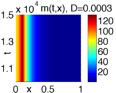
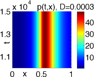
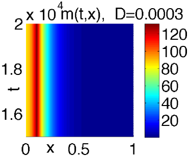
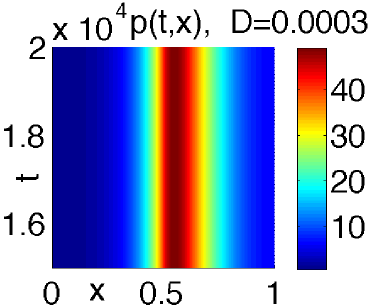
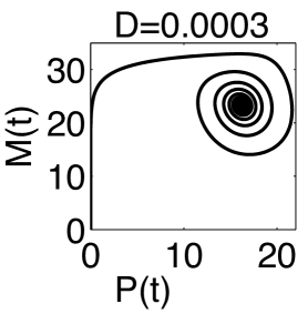
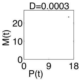
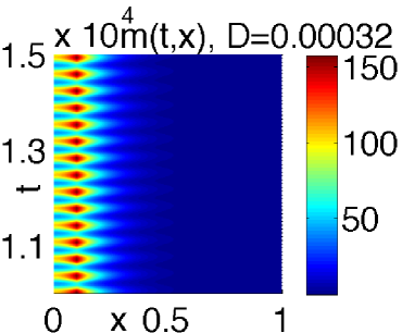
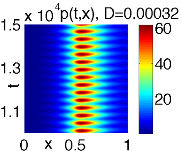
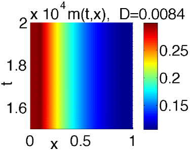
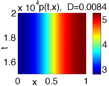
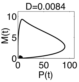
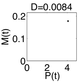
Numerical simulations of the model (5) (using the forward Euler scheme in time and a centred difference scheme in space, as well as the Dirac sequence in the form ฮดxMฮตโ€‹(x)=12โ€‹ฮตโ€‹(1+cosโก(ฯ€โ€‹(xโˆ’xM)/ฮต))subscriptsuperscript๐›ฟ๐œ€subscript๐‘ฅ๐‘€๐‘ฅ12๐œ€1๐œ‹๐‘ฅsubscript๐‘ฅ๐‘€๐œ€\delta^{\varepsilon}_{x_{M}}(x)=\frac{1}{2\varepsilon}(1+\cos(\pi(x-x_{M})/\varepsilon)) for |xโˆ’xM|<ฮต๐‘ฅsubscript๐‘ฅ๐‘€๐œ€|x-x_{M}|<\varepsilon and ฮดxMฮตโ€‹(x)=0subscriptsuperscript๐›ฟ๐œ€subscript๐‘ฅ๐‘€๐‘ฅ0\delta^{\varepsilon}_{x_{M}}(x)=0 for |xโˆ’xM|โ‰ฅฮต๐‘ฅsubscript๐‘ฅ๐‘€๐œ€|x-x_{M}|\geq\varepsilon) reveal that a stationary solution, stable for small values of the diffusion coefficient D๐ทD, becomes unstable for Dโ‰ฅD1,ฮตc๐ทsuperscriptsubscript๐ท1๐œ€๐‘D\geq D_{1,\varepsilon}^{c}, with D1,ฮตcโ‰ˆ3.117ร—10โˆ’4superscriptsubscript๐ท1๐œ€๐‘3.117superscript104D_{1,\varepsilon}^{c}\approx 3.117\times 10^{-4}, and again stable for D>D2,ฮตc๐ทsubscriptsuperscript๐ท๐‘2๐œ€D>D^{c}_{2,\varepsilon}, where D2,ฮตcโ‰ˆ7.885ร—10โˆ’3subscriptsuperscript๐ท๐‘2๐œ€7.885superscript103D^{c}_{2,\varepsilon}\approx 7.885\times 10^{-3}. For diffusion coefficients between the two critical values, i.e. Dโˆˆ[D1,ฮตc,D2,ฮตc]๐ทsuperscriptsubscript๐ท1๐œ€๐‘superscriptsubscript๐ท2๐œ€๐‘D\in[D_{1,\varepsilon}^{c},D_{2,\varepsilon}^{c}], numerical simulations show the existence of stable periodic solutions of the model (5). These scenarios are shown in Figs.ย 2-5.

Refer to caption
Refer to caption
Refer to caption
Refer to caption
Refer to caption
Refer to caption
Figure 2: First two rows: plots showing the spatio-temporal evolution of mRNA level, mโ€‹(t,x)๐‘š๐‘ก๐‘ฅm(t,x), and protein level, pโ€‹(t,x)๐‘๐‘ก๐‘ฅp(t,x), from numerical simulations of system (5) with zero initial conditions, with ฮต=10โˆ’3๐œ€superscript103\varepsilon=10^{-3}, D=0.0003๐ท0.0003D=0.0003, and tโˆˆ[104,2โ‹…104]๐‘กsuperscript104โ‹…2superscript104t\in[10^{4},2\cdot 10^{4}]. The plots show that the solutions tend to a steady-state. Bottom row: the corresponding phase-plots, where Mโ€‹(t)=โˆซ01mโ€‹(t,x)โ€‹๐‘‘x๐‘€๐‘กsuperscriptsubscript01๐‘š๐‘ก๐‘ฅdifferential-d๐‘ฅM(t)=\int_{0}^{1}m(t,x)dx and Pโ€‹(t)=โˆซ01pโ€‹(t,x)โ€‹๐‘‘x๐‘ƒ๐‘กsuperscriptsubscript01๐‘๐‘ก๐‘ฅdifferential-d๐‘ฅP(t)=\int_{0}^{1}p(t,x)dx. The figure on the left is for tโˆˆ[0,2ร—104]๐‘ก02superscript104t\in[0,2\times 10^{4}], and the figure on the right is for tโˆˆ[104,2ร—104]๐‘กsuperscript1042superscript104t\in[10^{4},2\times 10^{4}]. These show the trajectory converging to a fixed point, equivalent to the steady-state.
Refer to caption
Refer to caption
Refer to caption
Refer to caption
Refer to caption
Refer to caption
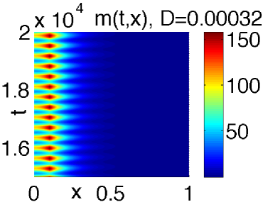
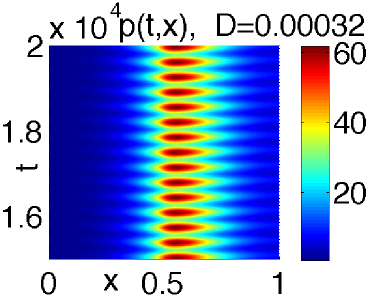
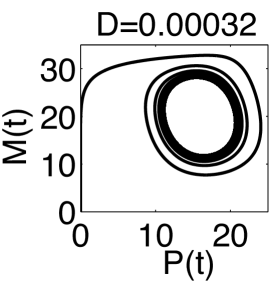
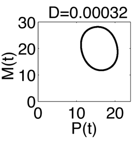
Figure 3: First two rows: plots showing the spatio-temporal evolution of mRNA level, mโ€‹(t,x)๐‘š๐‘ก๐‘ฅm(t,x), and protein level, pโ€‹(t,x)๐‘๐‘ก๐‘ฅp(t,x), from numerical simulations of system (5) with zero initial conditions, with ฮต=10โˆ’3๐œ€superscript103\varepsilon=10^{-3}, D=0.00032๐ท0.00032D=0.00032 and tโˆˆ[104,2ร—104]๐‘กsuperscript1042superscript104t\in[10^{4},2\times 10^{4}]. The plots show oscillatory solutions. Bottom row: the corresponding phase-plots, where Mโ€‹(t)=โˆซ01mโ€‹(t,x)โ€‹๐‘‘x๐‘€๐‘กsuperscriptsubscript01๐‘š๐‘ก๐‘ฅdifferential-d๐‘ฅM(t)=\int_{0}^{1}m(t,x)dx and Pโ€‹(t)=โˆซ01pโ€‹(t,x)โ€‹๐‘‘x๐‘ƒ๐‘กsuperscriptsubscript01๐‘๐‘ก๐‘ฅdifferential-d๐‘ฅP(t)=\int_{0}^{1}p(t,x)dx. The figure on the left is for tโˆˆ[0,2ร—104]๐‘ก02superscript104t\in[0,2\times 10^{4}], and the figure on the right is for tโˆˆ[104,2ร—104]๐‘กsuperscript1042superscript104t\in[10^{4},2\times 10^{4}]. These show the trajectory converging to a limit-cycle.
Refer to caption
Refer to caption
Refer to caption
Refer to caption
Refer to caption
Refer to caption
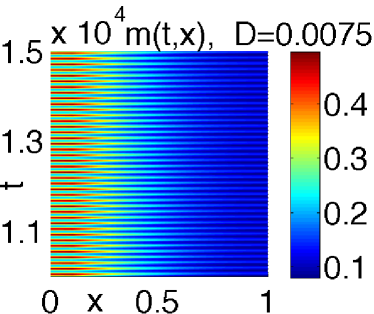
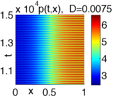
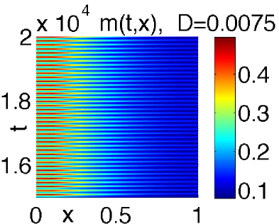
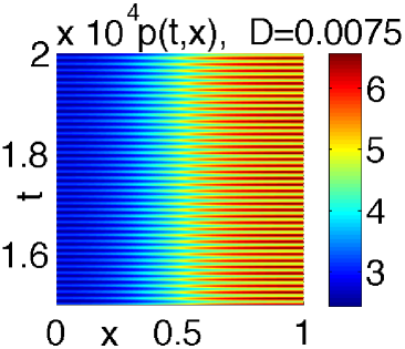
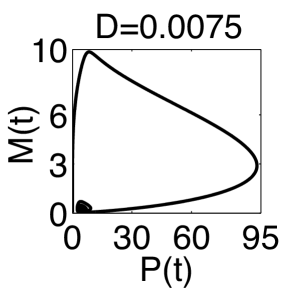
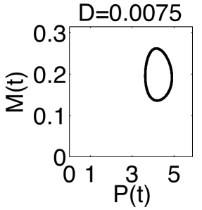
Figure 4: First two rows: plots showing the spatio-temporal evolution of mRNA level, mโ€‹(t,x)๐‘š๐‘ก๐‘ฅm(t,x), and protein level, pโ€‹(t,x)๐‘๐‘ก๐‘ฅp(t,x), from numerical simulations of system (5) with zero initial conditions, with ฮต=10โˆ’3๐œ€superscript103\varepsilon=10^{-3}, D=0.0075๐ท0.0075D=0.0075 and tโˆˆ[104,2ร—104]๐‘กsuperscript1042superscript104t\in[10^{4},2\times 10^{4}]. The plots show oscillatory solutions. Bottom row: the corresponding phase-plots, where Mโ€‹(t)=โˆซ01mโ€‹(t,x)โ€‹๐‘‘x๐‘€๐‘กsuperscriptsubscript01๐‘š๐‘ก๐‘ฅdifferential-d๐‘ฅM(t)=\int_{0}^{1}m(t,x)dx and Pโ€‹(t)=โˆซ01pโ€‹(t,x)โ€‹๐‘‘x๐‘ƒ๐‘กsuperscriptsubscript01๐‘๐‘ก๐‘ฅdifferential-d๐‘ฅP(t)=\int_{0}^{1}p(t,x)dx. The figure on the left is for tโˆˆ[0,2ร—104]๐‘ก02superscript104t\in[0,2\times 10^{4}], and the figure on the right is for tโˆˆ[104,2ร—104]๐‘กsuperscript1042superscript104t\in[10^{4},2\times 10^{4}]. These show the trajectory converging to a limit-cycle.
Refer to caption
Refer to caption
Refer to caption
Refer to caption
Refer to caption
Refer to caption
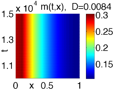
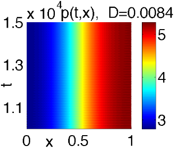
Figure 5: First two rows: plots showing the spatio-temporal evolution of mRNA level, mโ€‹(t,x)๐‘š๐‘ก๐‘ฅm(t,x), and protein level, pโ€‹(t,x)๐‘๐‘ก๐‘ฅp(t,x), from numerical simulations of system (5) with zero initial conditions, with ฮต=10โˆ’3๐œ€superscript103\varepsilon=10^{-3}, D=0.0084๐ท0.0084D=0.0084 and tโˆˆ[104,2ร—104]๐‘กsuperscript1042superscript104t\in[10^{4},2\times 10^{4}]. The plots show that the solutions tend to a steady-state. Bottom row: the corresponding phase-plots, where Mโ€‹(t)=โˆซ01mโ€‹(t,x)โ€‹๐‘‘x๐‘€๐‘กsuperscriptsubscript01๐‘š๐‘ก๐‘ฅdifferential-d๐‘ฅM(t)=\int_{0}^{1}m(t,x)dx and Pโ€‹(t)=โˆซ01pโ€‹(t,x)โ€‹๐‘‘x๐‘ƒ๐‘กsuperscriptsubscript01๐‘๐‘ก๐‘ฅdifferential-d๐‘ฅP(t)=\int_{0}^{1}p(t,x)dx. The figure on the left is for tโˆˆ[0,2ร—104]๐‘ก02superscript104t\in[0,2\times 10^{4}], and the figure on the right is for tโˆˆ[104,2ร—104]๐‘กsuperscript1042superscript104t\in[10^{4},2\times 10^{4}]. These show the trajectory converging to a fixed point, equivalent to the steady-state.

In the following sections we shall analyse the existence and stability of a family of periodic solutions bifurcating from the stationary solution. We shall show that at both critical values of the diffusion coefficient a supercritical Hopf bifurcation occurs.

3 Hopf Bifurcation Analysis

In this section we shall prove the existence of a Hopf bifurcation for the model (5) by showing that all conditions of the Hopf Bifurcation theorem are satisfied, see e.g. Crandall & Rabinowitz [6], Ize [29] or Kielhรถfer [34]. In order to achieve this, we examine first the stationary solutions of (5). A stationary solution uฮตโˆ—=(mฮตโˆ—,pฮตโˆ—)subscriptsuperscript๐‘ขโˆ—๐œ€subscriptsuperscript๐‘šโˆ—๐œ€subscriptsuperscript๐‘โˆ—๐œ€u^{\ast}_{\varepsilon}=(m^{\ast}_{\varepsilon},p^{\ast}_{\varepsilon}) of the system (5) satisfies the following one-dimensional boundary-value problem:

Dโ€‹d2โ€‹mฮตโˆ—dโ€‹x2+ฮฑmโ€‹fโ€‹(pฮตโˆ—)โ€‹ฮดxMฮตโ€‹(x)โˆ’ฮผโ€‹mฮตโˆ—=0ย inย โ€‹(0,1),Dโ€‹d2โ€‹pฮตโˆ—dโ€‹x2+ฮฑpโ€‹gโ€‹(x)โ€‹mฮตโˆ—โˆ’ฮผโ€‹pฮตโˆ—=0ย inย โ€‹(0,1),dโ€‹mฮตโˆ—โ€‹(0)dโ€‹x=dโ€‹mฮตโˆ—โ€‹(1)dโ€‹x=0,dโ€‹pฮตโˆ—โ€‹(0)dโ€‹x=dโ€‹pฮตโˆ—โ€‹(1)dโ€‹x=0.missing-subexpression๐ทsuperscript๐‘‘2subscriptsuperscript๐‘šโˆ—๐œ€๐‘‘superscript๐‘ฅ2subscript๐›ผ๐‘š๐‘“subscriptsuperscript๐‘โˆ—๐œ€subscriptsuperscript๐›ฟ๐œ€subscript๐‘ฅ๐‘€๐‘ฅ๐œ‡subscriptsuperscript๐‘šโˆ—๐œ€0ย inย 01missing-subexpression๐ทsuperscript๐‘‘2subscriptsuperscript๐‘โˆ—๐œ€๐‘‘superscript๐‘ฅ2subscript๐›ผ๐‘๐‘”๐‘ฅsubscriptsuperscript๐‘šโˆ—๐œ€๐œ‡subscriptsuperscript๐‘โˆ—๐œ€0ย inย 01missing-subexpressionformulae-sequence๐‘‘subscriptsuperscript๐‘šโˆ—๐œ€0๐‘‘๐‘ฅ๐‘‘subscriptsuperscript๐‘šโˆ—๐œ€1๐‘‘๐‘ฅ0๐‘‘subscriptsuperscript๐‘โˆ—๐œ€0๐‘‘๐‘ฅ๐‘‘subscriptsuperscript๐‘โˆ—๐œ€1๐‘‘๐‘ฅ0\displaystyle\begin{aligned} &D\frac{d^{2}m^{\ast}_{\varepsilon}}{dx^{2}}+\alpha_{m}\,f(p^{\ast}_{\varepsilon})\,\delta^{\varepsilon}_{x_{M}}(x)-\mu\,m^{\ast}_{\varepsilon}=0\qquad\text{ in }(0,1)\;,\\ &D\frac{d^{2}p^{\ast}_{\varepsilon}}{dx^{2}}+\alpha_{p}\,g(x)\,m^{\ast}_{\varepsilon}-\mu\,p^{\ast}_{\varepsilon}=0\qquad\hskip 32.72049pt\text{ in }(0,1)\;,\\ &\frac{dm^{\ast}_{\varepsilon}(0)}{dx}=\frac{dm^{\ast}_{\varepsilon}(1)}{dx}=0,\qquad\frac{dp^{\ast}_{\varepsilon}(0)}{dx}=\frac{dp^{\ast}_{\varepsilon}(1)}{dx}=0\;.\end{aligned} (7)

The operator ๐’œ~0=(Dโ€‹d2dโ€‹x2โˆ’ฮผ)subscript~๐’œ0๐ทsuperscript๐‘‘2๐‘‘superscript๐‘ฅ2๐œ‡\mathcal{\tilde{A}}_{0}=\big{(}D\dfrac{d^{2}}{dx^{2}}-\mu\big{)}, defined on the interval [0,1]01[0,1] and subject to the Neumann boundary conditions,

๐’Ÿโ€‹(๐’œ~0)={vโˆˆH2โ€‹(0,1):vโ€ฒโ€‹(0)=0,vโ€ฒโ€‹(1)=0},๐’Ÿsubscript~๐’œ0conditional-set๐‘ฃsuperscript๐ป201formulae-sequencesuperscript๐‘ฃโ€ฒ00superscript๐‘ฃโ€ฒ10\mathcal{D}(\mathcal{\tilde{A}}_{0})=\{v\in H^{2}(0,1):\,v^{\prime}(0)=0,\,v^{\prime}(1)=0\},

is invertible and solutions of the problem (7) can be defined as

mฮตโˆ—โ€‹(x,D)=ฮฑmโ€‹โˆซ01Gฮผโ€‹(x,y)โ€‹fโ€‹(pฮตโˆ—โ€‹(y,D))โ€‹ฮดxMฮตโ€‹(y)โ€‹๐‘‘y,pฮตโˆ—โ€‹(x,D)=ฮฑmโ€‹ฮฑpโ€‹โˆซ01gโ€‹(z)โ€‹Gฮผโ€‹(x,z)โ€‹โˆซ01Gฮผโ€‹(z,y)โ€‹fโ€‹(pฮตโˆ—โ€‹(y,D))โ€‹ฮดxMฮตโ€‹(y)โ€‹๐‘‘yโ€‹๐‘‘z,missing-subexpressionsubscriptsuperscript๐‘šโˆ—๐œ€๐‘ฅ๐ทsubscript๐›ผ๐‘šsuperscriptsubscript01subscript๐บ๐œ‡๐‘ฅ๐‘ฆ๐‘“subscriptsuperscript๐‘โˆ—๐œ€๐‘ฆ๐ทsuperscriptsubscript๐›ฟsubscript๐‘ฅ๐‘€๐œ€๐‘ฆdifferential-d๐‘ฆmissing-subexpressionsubscriptsuperscript๐‘โˆ—๐œ€๐‘ฅ๐ทsubscript๐›ผ๐‘šsubscript๐›ผ๐‘superscriptsubscript01๐‘”๐‘งsubscript๐บ๐œ‡๐‘ฅ๐‘งsuperscriptsubscript01subscript๐บ๐œ‡๐‘ง๐‘ฆ๐‘“subscriptsuperscript๐‘โˆ—๐œ€๐‘ฆ๐ทsuperscriptsubscript๐›ฟsubscript๐‘ฅ๐‘€๐œ€๐‘ฆdifferential-d๐‘ฆdifferential-d๐‘ง\displaystyle\begin{aligned} &m^{\ast}_{\varepsilon}(x,D)=\alpha_{m}\int_{0}^{1}G_{\mu}(x,y)f(p^{\ast}_{\varepsilon}(y,D))\delta_{x_{M}}^{\varepsilon}(y)\,dy\;,\\ &p^{\ast}_{\varepsilon}(x,D)=\alpha_{m}\alpha_{p}\int_{0}^{1}g(z)G_{\mu}(x,z)\int_{0}^{1}G_{\mu}(z,y)f(p^{\ast}_{\varepsilon}(y,D))\delta_{x_{M}}^{\varepsilon}(y)\,dy\,dz\;,\end{aligned} (8)

where

Gฮผโ€‹(y,x)={1(ฮผโ€‹D)1/2โ€‹sinhโก(ฮธ)โ€‹coshโก(ฮธโ€‹y)โ€‹coshโก(ฮธโ€‹(1โˆ’x))ย forย โ€‹โ€‰0<y<x<1,1(ฮผโ€‹D)1/2โ€‹sinhโก(ฮธ)โ€‹coshโก(ฮธโ€‹(1โˆ’y))โ€‹coshโก(ฮธโ€‹x)ย forย โ€‹โ€‰0<x<y<1,subscript๐บ๐œ‡๐‘ฆ๐‘ฅcases1superscript๐œ‡๐ท12๐œƒ๐œƒ๐‘ฆ๐œƒ1๐‘ฅย forย โ€‰0๐‘ฆ๐‘ฅ1otherwiseotherwiseotherwise1superscript๐œ‡๐ท12๐œƒ๐œƒ1๐‘ฆ๐œƒ๐‘ฅย forย โ€‰0๐‘ฅ๐‘ฆ1otherwiseG_{\mu}(y,x)=\begin{cases}\displaystyle{\frac{1}{(\mu D)^{1/2}\sinh(\theta)}}\cosh(\theta\,y)\cosh(\theta\,(1-x))\quad\text{ for }\,0<y<x<1\;,\\ \\ \displaystyle{\frac{1}{(\mu D)^{1/2}\sinh(\theta)}}\cosh(\theta\,(1-y))\cosh(\theta\,x)\quad\text{ for }\,0<x<y<1\;,\end{cases}

with ฮธ=(ฮผ/D)1/2๐œƒsuperscript๐œ‡๐ท12\theta=({\mu}/{D})^{1/2}, is the Greenโ€™s function satisfying the boundary-value problem

Dโ€‹Gyโ€‹yโˆ’ฮผโ€‹G=โˆ’ฮดxย inย โ€‹(0,1),Gyโ€‹(0,x)=Gyโ€‹(1,x)=0.formulae-sequence๐ทsubscript๐บ๐‘ฆ๐‘ฆ๐œ‡๐บsubscript๐›ฟ๐‘ฅย inย 01subscript๐บ๐‘ฆ0๐‘ฅsubscript๐บ๐‘ฆ1๐‘ฅ0DG_{yy}-\mu G=-\delta_{x}\quad\text{ in }\,(0,1),\qquad G_{y}(0,x)=G_{y}(1,x)=0.

Due to the boundedness of f๐‘“f for nonnegative pฮตโˆ—subscriptsuperscript๐‘โˆ—๐œ€p^{\ast}_{\varepsilon}, the continuous embedding of H1โ€‹(0,1)superscript๐ป101H^{1}(0,1) into Cโ€‹([0,1])๐ถ01C([0,1]) and the properties of the Dirac sequence, we obtain for nonnegative solutions of (7) the a priori estimates

โ€–mฮตโˆ—โ€–H1โ€‹(0,1)โ‰คC,โ€–mฮตโˆ—โ€–Cโ€‹([0,1])โ‰คC,โ€–pฮตโˆ—โ€–H1โ€‹(0,1)โ‰คC,โ€–pฮตโˆ—โ€–H2โ€‹(0,1)โ‰คC,formulae-sequencesubscriptnormsubscriptsuperscript๐‘šโˆ—๐œ€superscript๐ป101๐ถformulae-sequencesubscriptnormsubscriptsuperscript๐‘šโˆ—๐œ€๐ถ01๐ถformulae-sequencesubscriptnormsubscriptsuperscript๐‘โˆ—๐œ€superscript๐ป101๐ถsubscriptnormsubscriptsuperscript๐‘โˆ—๐œ€superscript๐ป201๐ถ\displaystyle\|m^{\ast}_{\varepsilon}\|_{H^{1}(0,1)}\leq C\;,\,\,\|m^{\ast}_{\varepsilon}\|_{C([0,1])}\leq C\;,\,\,\|p^{\ast}_{\varepsilon}\|_{H^{1}(0,1)}\leq C\;,\,\,\|p^{\ast}_{\varepsilon}\|_{H^{2}(0,1)}\leq C\;, (9)

with a constant C๐ถC independent of ฮต๐œ€\varepsilon.
From the second equation in (8) we have that

pฮตโˆ—โ€‹(x,D)=Kโ€‹(pฮตโˆ—โ€‹(x,D))subscriptsuperscript๐‘โˆ—๐œ€๐‘ฅ๐ท๐พsubscriptsuperscript๐‘โˆ—๐œ€๐‘ฅ๐ทp^{\ast}_{\varepsilon}(x,D)=K(p^{\ast}_{\varepsilon}(x,D)) (10)

with Kโ€‹(p)=ฮฑmโ€‹ฮฑpโ€‹(โˆ’๐’œ~0)โˆ’1โ€‹(gโ€‹(โˆ’๐’œ~0)โˆ’1โ€‹(ฮดxMฮตโ€‹fโ€‹(p)))๐พ๐‘subscript๐›ผ๐‘šsubscript๐›ผ๐‘superscriptsubscript~๐’œ01๐‘”superscriptsubscript~๐’œ01superscriptsubscript๐›ฟsubscript๐‘ฅ๐‘€๐œ€๐‘“๐‘K(p)=\alpha_{m}\alpha_{p}(-\mathcal{\tilde{A}}_{0})^{-1}\left(g(-\mathcal{\tilde{A}}_{0})^{-1}\big{(}\delta_{x_{M}}^{\varepsilon}f(p)\big{)}\right), where K:Cโ€‹([0,1])โ†’Cโ€‹([0,1]):๐พโ†’๐ถ01๐ถ01K:C([0,1])\to C([0,1]) is compact, since (โˆ’๐’œ~0)โˆ’1superscriptsubscript~๐’œ01(-\mathcal{\tilde{A}}_{0})^{-1} is compact. Consider a closed convex bounded subset D={pโˆˆCโ€‹([0,1]):โ€‰0โ‰คpโ€‹(x)โ‰คC+1โ€‹ย forย โ€‹xโˆˆ[0,1]}๐ทconditional-set๐‘๐ถ01โ€‰0๐‘๐‘ฅ๐ถ1ย forย ๐‘ฅ01D=\{p\in C([0,1]):\,0\leq p(x)\leq C+1\text{ for }x\in[0,1]\} of Cโ€‹([0,1])๐ถ01C([0,1]), where the constant C๐ถC is as in estimates (9). The estimates (9) and the fact that Kโ€‹(p)>0๐พ๐‘0K(p)>0 for pโ‰ฅ0๐‘0p\geq 0 imply pโˆ’Kโ€‹(p)โ‰ 0๐‘๐พ๐‘0p-K(p)\neq 0 for pโˆˆโˆ‚D๐‘๐ทp\in\partial D. Thus Leray-Schauder degree theory, e.g. Chapter 12.B in Smoller [60], guarantees the existence of a positive solution of (7). The linearised equations (7) at the steady state (mฮตโˆ—,pฮตโˆ—)subscriptsuperscript๐‘šโˆ—๐œ€subscriptsuperscript๐‘โˆ—๐œ€(m^{\ast}_{\varepsilon},p^{\ast}_{\varepsilon}) can be written

๐’œโ€‹u=0,๐’œ๐‘ข0\mathcal{A}u=0, (11)

where u=(u1,u2)๐‘ขsubscript๐‘ข1subscript๐‘ข2u=(u_{1},u_{2}) and ๐’œ=๐’œ0+๐’œ1๐’œsubscript๐’œ0subscript๐’œ1\mathcal{A}=\mathcal{A}_{0}+\mathcal{A}_{1} with the operator ๐’œ0subscript๐’œ0\mathcal{A}_{0} given as

๐’œ0=(Dโ€‹d2dโ€‹x2โˆ’ฮผ)โ€‹Isubscript๐’œ0๐ทsuperscript๐‘‘2๐‘‘superscript๐‘ฅ2๐œ‡๐ผ\mathcal{A}_{0}=\Big{(}D\dfrac{d^{2}}{dx^{2}}-\mu\Big{)}I (12)

on the interval [0,1]01[0,1], subject to the Neumann boundary conditions,

๐’Ÿโ€‹(๐’œ0)={vโˆˆH2โ€‹(0,1)ร—H2โ€‹(0,1):vโ€ฒโ€‹(0)=0,vโ€ฒโ€‹(1)=0},๐’Ÿsubscript๐’œ0conditional-set๐‘ฃsuperscript๐ป201superscript๐ป201formulae-sequencesuperscript๐‘ฃโ€ฒ00superscript๐‘ฃโ€ฒ10\mathcal{D}(\mathcal{A}_{0})=\{v\in H^{2}(0,1)\times H^{2}(0,1):\,v^{\prime}(0)=0,\,v^{\prime}(1)=0\},

and the bounded operator

๐’œ1=(0ฮฑmโ€‹fโ€ฒโ€‹(pฮตโˆ—โ€‹(x,D))โ€‹ฮดxMฮตโ€‹(x)ฮฑpโ€‹gโ€‹(x)0).subscript๐’œ1matrix0subscript๐›ผ๐‘šsuperscript๐‘“โ€ฒsubscriptsuperscript๐‘โˆ—๐œ€๐‘ฅ๐ทsubscriptsuperscript๐›ฟ๐œ€subscript๐‘ฅ๐‘€๐‘ฅsubscript๐›ผ๐‘๐‘”๐‘ฅ0\mathcal{A}_{1}=\begin{pmatrix}0&\alpha_{m}f^{\prime}(p^{\ast}_{\varepsilon}(x,D))\,\delta^{\varepsilon}_{x_{M}}(x)\\ \alpha_{p}g(x)&0\end{pmatrix}\;. (13)

If for a solution u=(u1,u2)๐‘ขsubscript๐‘ข1subscript๐‘ข2u=(u_{1},u_{2}) of (11) we have u2โ€‹(x)=0subscript๐‘ข2๐‘ฅ0u_{2}(x)=0 in (xMโˆ’ฮต,xM+ฮต)subscript๐‘ฅ๐‘€๐œ€subscript๐‘ฅ๐‘€๐œ€(x_{M}-\varepsilon,x_{M}+\varepsilon), then uโ‰ก(0,0)๐‘ข00u\equiv(0,0) and ๐’œ๐’œ\mathcal{A} is invertible. Suppose there exists a non-trivial solution of (11) with u2โ€‹(x)โ‰ 0subscript๐‘ข2๐‘ฅ0u_{2}(x)\neq 0 in (xMโˆ’ฮต,xM+ฮต)subscript๐‘ฅ๐‘€๐œ€subscript๐‘ฅ๐‘€๐œ€(x_{M}-\varepsilon,x_{M}+\varepsilon). Using the continuity of u2subscript๐‘ข2u_{2}, we can assume u2โ€‹(x)>0subscript๐‘ข2๐‘ฅ0u_{2}(x)>0 in (xMโˆ’ฮต,xM+ฮต)subscript๐‘ฅ๐‘€๐œ€subscript๐‘ฅ๐‘€๐œ€(x_{M}-\varepsilon,x_{M}+\varepsilon) for small ฮต๐œ€\varepsilon. Then, the properties of f๐‘“f and positivity of (โˆ’๐’œ~0)subscript~๐’œ0(-\mathcal{\tilde{A}}_{0}) and of the steady state (mฮตโˆ—,pฮตโˆ—)subscriptsuperscript๐‘šโˆ—๐œ€subscriptsuperscript๐‘โˆ—๐œ€(m^{\ast}_{\varepsilon},p^{\ast}_{\varepsilon}) ensure

u2โ€‹(x)โˆ’ฮฑmโ€‹ฮฑpโ€‹(โˆ’๐’œ~0)โˆ’1โ€‹(gโ€‹(โˆ’๐’œ~0)โˆ’1โ€‹(fโ€ฒโ€‹(pฮตโˆ—)โ€‹ฮดxMฮตโ€‹u2))โ€‹(x)>0โ€‹ย forย โ€‹xโˆˆ(xMโˆ’ฮต,xM+ฮต).subscript๐‘ข2๐‘ฅsubscript๐›ผ๐‘šsubscript๐›ผ๐‘superscriptsubscript~๐’œ01๐‘”superscriptsubscript~๐’œ01superscript๐‘“โ€ฒsubscriptsuperscript๐‘โˆ—๐œ€subscriptsuperscript๐›ฟ๐œ€subscript๐‘ฅ๐‘€subscript๐‘ข2๐‘ฅ0ย forย ๐‘ฅsubscript๐‘ฅ๐‘€๐œ€subscript๐‘ฅ๐‘€๐œ€u_{2}(x)-\alpha_{m}\alpha_{p}(-\mathcal{\tilde{A}}_{0})^{-1}\Big{(}g\,(-\mathcal{\tilde{A}}_{0})^{-1}\big{(}f^{\prime}(p^{\ast}_{\varepsilon})\delta^{\varepsilon}_{x_{M}}u_{2}\big{)}\Big{)}(x)>0\,\,\text{ for }x\in(x_{M}-\varepsilon,x_{M}+\varepsilon)\;.

This last inequality implies a contradiction, since u2subscript๐‘ข2u_{2} was a solution of (11). Therefore, ๐’œ๐’œ\mathcal{A} is invertible for every Dโˆˆ[d1,d2]๐ทsubscript๐‘‘1subscript๐‘‘2D\in[d_{1},d_{2}]. Thus for every fixed small ฮต>0๐œ€0\varepsilon>0 we have a family in Dโˆˆ[d1,d2]๐ทsubscript๐‘‘1subscript๐‘‘2D\in[d_{1},d_{2}] of isolated positive stationary solutions (mฮตโˆ—โ€‹(x,D),pฮตโˆ—โ€‹(x,D))โˆˆH2โ€‹(0,1)ร—H2โ€‹(0,1)subscriptsuperscript๐‘šโˆ—๐œ€๐‘ฅ๐ทsubscriptsuperscript๐‘โˆ—๐œ€๐‘ฅ๐ทsuperscript๐ป201superscript๐ป201(m^{\ast}_{\varepsilon}(x,D),p^{\ast}_{\varepsilon}(x,D))\in H^{2}(0,1)\times H^{2}(0,1) of (5).

The a priori estimates imply the weak convergences mฮตโˆ—โ‡€m0โˆ—โ‡€subscriptsuperscript๐‘šโˆ—๐œ€subscriptsuperscript๐‘šโˆ—0m^{\ast}_{\varepsilon}\rightharpoonup m^{\ast}_{0} in H1โ€‹(0,1)superscript๐ป101H^{1}(0,1) and pฮตโˆ—โ‡€p0โˆ—โ‡€subscriptsuperscript๐‘โˆ—๐œ€subscriptsuperscript๐‘โˆ—0p^{\ast}_{\varepsilon}\rightharpoonup p^{\ast}_{0} in H2โ€‹(0,1)superscript๐ป201H^{2}(0,1), and, by the compact embedding of H1โ€‹(0,1)superscript๐ป101H^{1}(0,1) in Cโ€‹([0,1])๐ถ01C([0,1]) and of H2โ€‹(0,1)superscript๐ป201H^{2}(0,1) in C1โ€‹([0,1])superscript๐ถ101C^{1}([0,1]), also strong convergence in Cโ€‹([0,1])๐ถ01C([0,1]) and in C1โ€‹([0,1])superscript๐ถ101C^{1}([0,1]) as ฮตโ†’0โ†’๐œ€0\varepsilon\to 0, respectively, where

m0โˆ—โ€‹(x,D)=ฮฑmโ€‹Gฮผโ€‹(x,xM)โ€‹fโ€‹(p0โˆ—โ€‹(xM,D)),p0โˆ—โ€‹(x,D)=ฮฑmโ€‹ฮฑpโ€‹fโ€‹(p0โˆ—โ€‹(xM,D))โ€‹โˆซ01gโ€‹(y)โ€‹Gฮผโ€‹(x,y)โ€‹Gฮผโ€‹(y,xM)โ€‹๐‘‘y,missing-subexpressionsubscriptsuperscript๐‘šโˆ—0๐‘ฅ๐ทsubscript๐›ผ๐‘šsubscript๐บ๐œ‡๐‘ฅsubscript๐‘ฅ๐‘€๐‘“subscriptsuperscript๐‘โˆ—0subscript๐‘ฅ๐‘€๐ทmissing-subexpressionsubscriptsuperscript๐‘โˆ—0๐‘ฅ๐ทsubscript๐›ผ๐‘šsubscript๐›ผ๐‘๐‘“subscriptsuperscript๐‘โˆ—0subscript๐‘ฅ๐‘€๐ทsuperscriptsubscript01๐‘”๐‘ฆsubscript๐บ๐œ‡๐‘ฅ๐‘ฆsubscript๐บ๐œ‡๐‘ฆsubscript๐‘ฅ๐‘€differential-d๐‘ฆ\displaystyle\begin{aligned} &m^{\ast}_{0}(x,D)=\alpha_{m}G_{\mu}(x,x_{M})f(p^{\ast}_{0}(x_{M},D))\;,\\ &p^{\ast}_{0}(x,D)=\alpha_{m}\alpha_{p}f(p^{\ast}_{0}(x_{M},D))\int_{0}^{1}g(y)\,G_{\mu}(x,y)\,G_{\mu}(y,x_{M})\,dy,\;\end{aligned} (14)

is a solution of the model (7) with the Delta distribution ฮดxMsubscript๐›ฟsubscript๐‘ฅ๐‘€\delta_{x_{M}} instead of the Dirac sequence ฮดxMฮตsubscriptsuperscript๐›ฟ๐œ€subscript๐‘ฅ๐‘€\delta^{\varepsilon}_{x_{M}}. Since xM<lsubscript๐‘ฅ๐‘€๐‘™x_{M}<l and gโ€‹(y)=0๐‘”๐‘ฆ0g(y)=0 for 0โ‰คy<l0๐‘ฆ๐‘™0\leq y<l, we have

Gฮผโ€‹(y,xM)=1(ฮผโ€‹D)1/2โ€‹sinhโก(ฮธ)โ€‹coshโก(ฮธโ€‹(1โˆ’y))โ€‹coshโก(ฮธโ€‹xM),xM<y<1,formulae-sequencesubscript๐บ๐œ‡๐‘ฆsubscript๐‘ฅ๐‘€1superscript๐œ‡๐ท12๐œƒ๐œƒ1๐‘ฆ๐œƒsubscript๐‘ฅ๐‘€subscript๐‘ฅ๐‘€๐‘ฆ1G_{\mu}(y,x_{M})=\frac{1}{(\mu D)^{1/2}\sinh(\theta)}\cosh(\theta(1-y))\cosh(\theta x_{M}),\quad x_{M}<y<1,\quad

where ฮธ=(ฮผ/D)1/2๐œƒsuperscript๐œ‡๐ท12\theta=\left(\mu/D\right)^{1/2} and, using gโ€‹(y)=1๐‘”๐‘ฆ1g(y)=1 for lโ‰คyโ‰ค1๐‘™๐‘ฆ1l\leq y\leq 1, we obtain

p0โˆ—(x,D)=ฮฑmโ€‹ฮฑpโ€‹fโ€‹(p0โˆ—โ€‹(xM,D))2โ€‹ฮผโ€‹Dโ€‹sinh2โก(ฮธ)cosh(ฮธxM)ร—\displaystyle p^{\ast}_{0}(x,D)=\frac{\alpha_{m}\alpha_{p}f(p^{\ast}_{0}(x_{M},D))}{2\mu D\sinh^{2}(\theta)}\cosh(\theta x_{M})\times
ร—[cosh(ฮธ(1โˆ’x))(cosh(ฮธ)y|lxโˆ’12โ€‹ฮธsinh(ฮธ(1โˆ’2y))|lx)x>l\displaystyle\times\Big{[}\cosh(\theta(1-x))\Big{(}\cosh(\theta)y\Big{|}_{l}^{x}-\frac{1}{2\theta}\sinh(\theta(1-2y))\Big{|}_{l}^{x}\Big{)}_{x>l}
+cosh(ฮธx)(y|maxโก{x,l}1โˆ’12โ€‹ฮธsinh(2ฮธ(1โˆ’y))|maxโก{x,l}1)].\displaystyle+\cosh(\theta x)\Big{(}y\Big{|}_{\max\{x,l\}}^{1}-\frac{1}{2\theta}\sinh(2\theta(1-y))\Big{|}^{1}_{\max\{x,l\}}\Big{)}\Big{]}\;.

It can be shown numerically that the nonlinear equation

p0โˆ—โ€‹(xM,D)=fโ€‹(p0โˆ—โ€‹(xM,D))โ€‹ฮฑpโ€‹ฮฑm4โ€‹cosh2โก(ฮธโ€‹xM)ฮผโ€‹Dโ€‹ฮธโ€‹sinh2โก(ฮธ)โ€‹[ฮธ+sinhโก(ฮธ)]subscriptsuperscript๐‘โˆ—0subscript๐‘ฅ๐‘€๐ท๐‘“subscriptsuperscript๐‘โˆ—0subscript๐‘ฅ๐‘€๐ทsubscript๐›ผ๐‘subscript๐›ผ๐‘š4superscript2๐œƒsubscript๐‘ฅ๐‘€๐œ‡๐ท๐œƒsuperscript2๐œƒdelimited-[]๐œƒ๐œƒ\displaystyle p^{\ast}_{0}(x_{M},D)=f(p^{\ast}_{0}(x_{M},D))\frac{\alpha_{p}\alpha_{m}}{4}\frac{\cosh^{2}(\theta\,x_{M})}{\mu\,D\,\theta\,\sinh^{2}(\theta)}\Big{[}\theta+\sinh(\theta)\Big{]} (15)

has only one positive solution for all values of Dโˆˆ[d1,d2]๐ทsubscript๐‘‘1subscript๐‘‘2D\in[d_{1},d_{2}].

Thus, since m0โˆ—โ€‹(x,D)subscriptsuperscript๐‘šโˆ—0๐‘ฅ๐ทm^{\ast}_{0}(x,D) and p0โˆ—โ€‹(x,D)subscriptsuperscript๐‘โˆ—0๐‘ฅ๐ทp^{\ast}_{0}(x,D) are uniquely defined by p0โˆ—โ€‹(xM,D)subscriptsuperscript๐‘โˆ—0subscript๐‘ฅ๐‘€๐ทp^{\ast}_{0}(x_{M},D), for every Dโˆˆ[d1,d2]๐ทsubscript๐‘‘1subscript๐‘‘2D\in[d_{1},d_{2}] we have a unique positive solution of (7) with ฮต=0๐œ€0\varepsilon=0. Then the strong convergence of mฮตโˆ—โ†’m0โˆ—โ†’subscriptsuperscript๐‘šโˆ—๐œ€subscriptsuperscript๐‘šโˆ—0m^{\ast}_{\varepsilon}\to m^{\ast}_{0}, pฮตโˆ—โ†’p0โˆ—โ†’subscriptsuperscript๐‘โˆ—๐œ€subscriptsuperscript๐‘โˆ—0p^{\ast}_{\varepsilon}\to p^{\ast}_{0} as ฮตโ†’0โ†’๐œ€0\varepsilon\to 0 in Cโ€‹([0,1])๐ถ01C([0,1]) and the fact that nonnegative steady states (mฮตโˆ—,pฮตโˆ—)subscriptsuperscript๐‘šโˆ—๐œ€subscriptsuperscript๐‘โˆ—๐œ€(m^{\ast}_{\varepsilon},p^{\ast}_{\varepsilon}) are isolated imply the uniqueness of the positive steady state of (5) for small ฮต>0๐œ€0\varepsilon>0 and Dโˆˆ[d1,d2]๐ทsubscript๐‘‘1subscript๐‘‘2D\in[d_{1},d_{2}].

Before carrying out our analysis, to better understand the structure of the stationary solutions of (5) we can consider their structure under extreme values of the diffusion coefficient D๐ทD. For very small diffusion coefficients Dโ‰ช1much-less-than๐ท1D\ll 1, in the zero-order approximation we obtain

0=ฮฑmโ€‹fโ€‹(pฮตโˆ—)โ€‹ฮดxMฮตโ€‹(x)โˆ’ฮผโ€‹mฮตโˆ—,0subscript๐›ผ๐‘š๐‘“subscriptsuperscript๐‘โˆ—๐œ€subscriptsuperscript๐›ฟ๐œ€subscript๐‘ฅ๐‘€๐‘ฅ๐œ‡subscriptsuperscript๐‘šโˆ—๐œ€\displaystyle 0=\alpha_{m}\,f(p^{\ast}_{\varepsilon})\delta^{\varepsilon}_{x_{M}}(x)-\mu\,m^{\ast}_{\varepsilon}\;,\quad 0=ฮฑpโ€‹gโ€‹(x)โ€‹mฮตโˆ—โˆ’ฮผโ€‹pฮตโˆ—ย inย โ€‹(0,1).0subscript๐›ผ๐‘๐‘”๐‘ฅsubscriptsuperscript๐‘šโˆ—๐œ€๐œ‡subscriptsuperscript๐‘โˆ—๐œ€ย inย 01\displaystyle 0=\alpha_{p}\,g(x)\,m^{\ast}_{\varepsilon}-\mu\,p^{\ast}_{\varepsilon}\quad\text{ in }(0,1)\;.

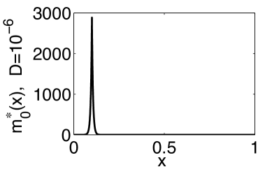
Since gโ€‹(x)=0๐‘”๐‘ฅ0g(x)=0 for xโˆˆ[0,l)๐‘ฅ0๐‘™x\in[0,l), the second equation yields that pฮตโˆ—โ€‹(x,D)=0subscriptsuperscript๐‘โˆ—๐œ€๐‘ฅ๐ท0p^{\ast}_{\varepsilon}(x,D)=0 in [0,l)0๐‘™[0,l) and thus mฮตโˆ—โ€‹(x,D)=ฮฑmฮผโ€‹ฮดxMฮตโ€‹(x)subscriptsuperscript๐‘šโˆ—๐œ€๐‘ฅ๐ทsubscript๐›ผ๐‘š๐œ‡subscriptsuperscript๐›ฟ๐œ€subscript๐‘ฅ๐‘€๐‘ฅm^{\ast}_{\varepsilon}(x,D)=\frac{\alpha_{m}}{\mu}\delta^{\varepsilon}_{x_{M}}(x) in [0,1]01[0,1]. Using the fact that xMโˆˆ(0,l)subscript๐‘ฅ๐‘€0๐‘™x_{M}\in(0,l) we obtain for sufficiently small ฮต>0๐œ€0\varepsilon>0 that mฮตโˆ—โ€‹(x,D)=0subscriptsuperscript๐‘šโˆ—๐œ€๐‘ฅ๐ท0m^{\ast}_{\varepsilon}(x,D)=0 for xโˆˆ[l,1]๐‘ฅ๐‘™1x\in[l,1] and thus pฮตโˆ—โ€‹(x,D)=0subscriptsuperscript๐‘โˆ—๐œ€๐‘ฅ๐ท0p^{\ast}_{\varepsilon}(x,D)=0 in [0,1]01[0,1]. Therefore for very small D๐ทD we have localisation of mRNA concentration around xMsubscript๐‘ฅ๐‘€x_{M}, whereas the concentration of protein is approximately zero everywhere in [0,1]01[0,1].

For large diffusion coefficients, i.e. Dโ‰ซ1much-greater-than๐ท1D\gg 1 and therefore 1/Dโ‰ช1much-less-than1๐ท11/D\ll 1, we have

0=d2โ€‹mฮตโˆ—dโ€‹x2+1Dโ€‹(ฮฑmโ€‹fโ€‹(pฮตโˆ—)โ€‹ฮดxMฮตโ€‹(x)โˆ’ฮผโ€‹mฮตโˆ—)ย inย โ€‹(0,1),0superscript๐‘‘2superscriptsubscript๐‘š๐œ€โˆ—๐‘‘superscript๐‘ฅ21๐ทsubscript๐›ผ๐‘š๐‘“subscriptsuperscript๐‘โˆ—๐œ€subscriptsuperscript๐›ฟ๐œ€subscript๐‘ฅ๐‘€๐‘ฅ๐œ‡subscriptsuperscript๐‘šโˆ—๐œ€ย inย 01\displaystyle 0=\frac{d^{2}m_{\varepsilon}^{\ast}}{dx^{2}}+\frac{1}{D}\big{(}\alpha_{m}\,f(p^{\ast}_{\varepsilon})\delta^{\varepsilon}_{x_{M}}(x)-\mu\,m^{\ast}_{\varepsilon}\big{)}\quad\text{ in }(0,1)\;,
0=d2โ€‹pฮตโˆ—dโ€‹x2+1Dโ€‹(ฮฑpโ€‹gโ€‹(x)โ€‹mฮตโˆ—โˆ’ฮผโ€‹pฮตโˆ—)ย inย โ€‹(0,1),0superscript๐‘‘2superscriptsubscript๐‘๐œ€โˆ—๐‘‘superscript๐‘ฅ21๐ทsubscript๐›ผ๐‘๐‘”๐‘ฅsubscriptsuperscript๐‘šโˆ—๐œ€๐œ‡subscriptsuperscript๐‘โˆ—๐œ€ย inย 01\displaystyle 0=\frac{d^{2}p_{\varepsilon}^{\ast}}{dx^{2}}+\frac{1}{D}\big{(}\alpha_{p}\,g(x)\,m^{\ast}_{\varepsilon}-\mu\,p^{\ast}_{\varepsilon}\big{)}\quad\hskip 31.2982pt\text{ in }(0,1)\;,
dโ€‹mฮตโˆ—dโ€‹xโ€‹(0)=dโ€‹mฮตโˆ—dโ€‹xโ€‹(1)=0,dโ€‹pฮตโˆ—dโ€‹xโ€‹(0)=dโ€‹pฮตโˆ—dโ€‹xโ€‹(1)=0.formulae-sequence๐‘‘subscriptsuperscript๐‘šโˆ—๐œ€๐‘‘๐‘ฅ0๐‘‘subscriptsuperscript๐‘šโˆ—๐œ€๐‘‘๐‘ฅ10๐‘‘subscriptsuperscript๐‘โˆ—๐œ€๐‘‘๐‘ฅ0๐‘‘subscriptsuperscript๐‘โˆ—๐œ€๐‘‘๐‘ฅ10\displaystyle\frac{dm^{\ast}_{\varepsilon}}{dx}(0)=\frac{dm^{\ast}_{\varepsilon}}{dx}(1)=0,\qquad\frac{dp^{\ast}_{\varepsilon}}{dx}(0)=\frac{dp^{\ast}_{\varepsilon}}{dx}(1)=0\;.

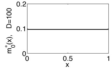
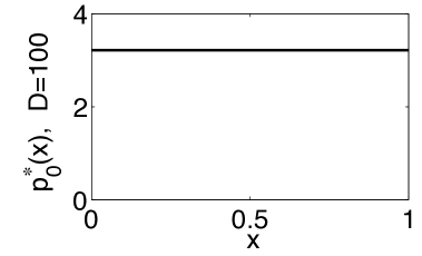
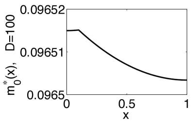
Thus mฮตโˆ—โ€‹(x,D)โ‰ˆconstsubscriptsuperscript๐‘šโˆ—๐œ€๐‘ฅ๐ทconstm^{\ast}_{\varepsilon}(x,D)\approx\text{const} and pฮตโˆ—โ€‹(x,D)โ‰ˆconstsubscriptsuperscript๐‘โˆ—๐œ€๐‘ฅ๐ทconstp^{\ast}_{\varepsilon}(x,D)\approx\text{const}.

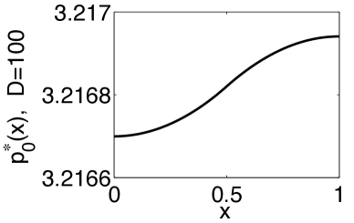
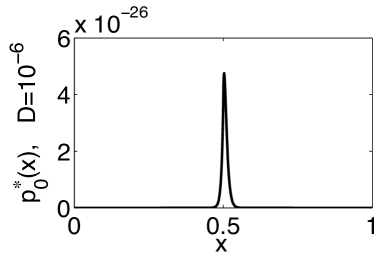
Representative stationary solutions, calculated numerically from (14), in the cases D=10โˆ’6โ‰ช1๐ทsuperscript106much-less-than1D=10^{-6}\ll 1 and D=100โ‰ซ1๐ท100much-greater-than1D=100\gg 1 can be seen in Figureย 6, confirming the preceding analysis.
Refer to caption
Refer to caption
Refer to caption
Refer to caption
Refer to caption
Refer to caption
Figure 6: Plots showing representative stationary solutions of the system (14), i.e. mRNA (left plot) and protein (right plot) steady-state concentrations, for D=10โˆ’6๐ทsuperscript106D=10^{-6} (top row) and D=100๐ท100D=100 (middle row, bottom row). The bottom row shows the stationary solution for D=100๐ท100D=100 at higher resolution.

Now, to study the linearized stability of the steady-state solution of the nonlinear model (5) we shall apply a version of Theorems 5.1.1 and 5.1.3 in Henry [25] adapted for our situation. We can write the system (5) in the Hilbert space X=L2โ€‹(0,1)โŠ—L2โ€‹(0,1)๐‘‹tensor-productsuperscript๐ฟ201superscript๐ฟ201X=L^{2}(0,1)\otimes L^{2}(0,1) as

โˆ‚tu=๐’œ0โ€‹u+f~โ€‹(u),subscript๐‘ก๐‘ขsubscript๐’œ0๐‘ข~๐‘“๐‘ข\partial_{t}u=\mathcal{A}_{0}u+\tilde{f}(u), (16)

where u=(m,p)T๐‘ขsuperscript๐‘š๐‘๐‘‡u=(m,p)^{T}, the operator ๐’œ0subscript๐’œ0\mathcal{A}_{0} is defined in (12) and f~โ€‹(u)=(ฮฑmโ€‹fโ€‹(p)โ€‹ฮดxMฮตโ€‹(x),ฮฑpโ€‹gโ€‹(x)โ€‹m)T~๐‘“๐‘ขsuperscriptsubscript๐›ผ๐‘š๐‘“๐‘subscriptsuperscript๐›ฟ๐œ€subscript๐‘ฅ๐‘€๐‘ฅsubscript๐›ผ๐‘๐‘”๐‘ฅ๐‘š๐‘‡\tilde{f}(u)=(\alpha_{m}f(p)\delta^{\varepsilon}_{x_{M}}(x),\alpha_{p}g(x)m)^{T}. The operator โˆ’๐’œ0subscript๐’œ0-\mathcal{A}_{0} is sectorial with ฯƒโ€‹(๐’œ0)โŠ‚(โˆ’โˆž,โˆ’ฮผ]๐œŽsubscript๐’œ0๐œ‡\sigma(\mathcal{A}_{0})\subset(-\infty,-\mu] and we can introduce interpolation spaces Xs=((โˆ’๐’œ0)s)superscript๐‘‹๐‘ superscriptsubscript๐’œ0๐‘ X^{s}=\mathcal{(}(-\mathcal{A}_{0})^{s}), each of which is a Hilbert subspace of H2โ€‹sโ€‹(0,1)ร—H2โ€‹sโ€‹(0,1)superscript๐ป2๐‘ 01superscript๐ป2๐‘ 01H^{2s}(0,1)\times H^{2s}(0,1). The function f~:โ„+2โ†’โ„+2:~๐‘“โ†’subscriptsuperscriptโ„2subscriptsuperscriptโ„2\tilde{f}:\mathbb{R}^{2}_{+}\to\mathbb{R}^{2}_{+} is smooth and admits the representation

f~โ€‹(y+z)=f~โ€‹(y)+Bโ€‹(y)โ€‹z+rโ€‹(y,z),~๐‘“๐‘ฆ๐‘ง~๐‘“๐‘ฆ๐ต๐‘ฆ๐‘ง๐‘Ÿ๐‘ฆ๐‘ง\tilde{f}(y+z)=\tilde{f}(y)+B(y)z+r(y,z),

where the remainder satisfies the estimate

โ€–rโ€‹(y,z)โ€–โ„2โ‰คCฮตโ€‹(y)โ€‹โ€–zโ€–โ„22,subscriptnorm๐‘Ÿ๐‘ฆ๐‘งsuperscriptโ„2subscript๐ถ๐œ€๐‘ฆsubscriptsuperscriptnorm๐‘ง2superscriptโ„2\|r(y,z)\|_{\mathbb{R}^{2}}\leq C_{\varepsilon}(y)\|z\|^{2}_{\mathbb{R}^{2}},

in a neighbourhood of any point yโˆˆโ„+2๐‘ฆsubscriptsuperscriptโ„2y\in\mathbb{R}^{2}_{+}, and

Bโ€‹(y)=(0ฮฑmโ€‹fโ€ฒโ€‹(y2)โ€‹ฮดxMฮตฮฑpโ€‹gโ€‹(x)0).๐ต๐‘ฆmatrix0subscript๐›ผ๐‘šsuperscript๐‘“โ€ฒsubscript๐‘ฆ2subscriptsuperscript๐›ฟ๐œ€subscript๐‘ฅ๐‘€subscript๐›ผ๐‘๐‘”๐‘ฅ0B(y)=\begin{pmatrix}0&\alpha_{m}f^{\prime}(y_{2})\delta^{\varepsilon}_{x_{M}}\\ \alpha_{p}g(x)&0\end{pmatrix}.

For a positive steady state uฮตโˆ—โ€‹(x,D)=(mฮตโˆ—โ€‹(x,D),pฮตโˆ—โ€‹(x,D))Tsubscriptsuperscript๐‘ขโˆ—๐œ€๐‘ฅ๐ทsuperscriptsubscriptsuperscript๐‘šโˆ—๐œ€๐‘ฅ๐ทsubscriptsuperscript๐‘โˆ—๐œ€๐‘ฅ๐ท๐‘‡u^{\ast}_{\varepsilon}(x,D)=(m^{\ast}_{\varepsilon}(x,D),p^{\ast}_{\varepsilon}(x,D))^{T}, with uฮตโˆ—โˆˆH1โ€‹(0,1)ร—H2โ€‹(0,1)subscriptsuperscript๐‘ขโˆ—๐œ€superscript๐ป101superscript๐ป201u^{\ast}_{\varepsilon}\in H^{1}(0,1)\times H^{2}(0,1), we obtain that Bโ€‹(uฮตโˆ—)๐ตsubscriptsuperscript๐‘ขโˆ—๐œ€B(u^{\ast}_{\varepsilon}) is a bounded linear operator from Xssuperscript๐‘‹๐‘ X^{s} to X๐‘‹X for each sโˆˆ(0,1)๐‘ 01s\in(0,1). The estimate for the remainder implies

โ€–rโ€‹(uฮตโˆ—,z)โ€–Xโ‰คCฮตโ€‹โ€–zโ€–X2โ‰คCฮตโ€‹โ€–zโ€–Xs2=oโ€‹(โ€–zโ€–Xs)โ†’0ย asย โ€–zโ€–Xsโ†’0,formulae-sequencesubscriptnorm๐‘Ÿsubscriptsuperscript๐‘ขโˆ—๐œ€๐‘ง๐‘‹subscript๐ถ๐œ€subscriptsuperscriptnorm๐‘ง2๐‘‹subscript๐ถ๐œ€subscriptsuperscriptnorm๐‘ง2superscript๐‘‹๐‘ ๐‘œsubscriptnorm๐‘งsuperscript๐‘‹๐‘ โ†’0โ†’ย asย subscriptnorm๐‘งsuperscript๐‘‹๐‘ 0\|r(u^{\ast}_{\varepsilon},z)\|_{X}\leq C_{\varepsilon}\|z\|^{2}_{X}\leq C_{\varepsilon}\|z\|^{2}_{X^{s}}=o(\|z\|_{X^{s}})\to 0\quad\text{ as }\quad\|z\|_{X^{s}}\to 0,

for every fixed ฮต>0๐œ€0\varepsilon>0. Notice that for sโˆˆ[1/2,1)๐‘ 121s\in[1/2,1), due to the properties of the Dirac sequence and the embedding of H1โ€‹(0,1)superscript๐ป101H^{1}(0,1) into Cโ€‹([0,1])๐ถ01C([0,1]), we have the estimates for B๐ตB and r๐‘Ÿr independent of ฮต๐œ€\varepsilon, i.e.

โ€–Bโ€‹(uฮตโˆ—)โ€‹zโ€–Xโ‰คCโ€‹โ€–zโ€–Xs,โ€–rโ€‹(uฮตโˆ—,z)โ€–Xโ‰คCโ€‹โ€–zโ€–Xs2formulae-sequencesubscriptnorm๐ตsubscriptsuperscript๐‘ขโˆ—๐œ€๐‘ง๐‘‹๐ถsubscriptnorm๐‘งsuperscript๐‘‹๐‘ subscriptnorm๐‘Ÿsubscriptsuperscript๐‘ขโˆ—๐œ€๐‘ง๐‘‹๐ถsubscriptsuperscriptnorm๐‘ง2superscript๐‘‹๐‘ \|B(u^{\ast}_{\varepsilon})z\|_{X}\leq C\|z\|_{X^{s}},\quad\quad\|r(u^{\ast}_{\varepsilon},z)\|_{X}\leq C\|z\|^{2}_{X^{s}}

with a constant C๐ถC independent of ฮต๐œ€\varepsilon.

Thus, all assumptions of the Theorems 5.1.1 and 5.1.3 in Henry [25] are satisfied and to analyse the linearized stability of the stationary solution of the system (5) we shall study the eigenvalue problem:

ฮปโ€‹mยฏฮต=Dโ€‹mยฏxโ€‹xฮต+ฮฑmโ€‹fโ€ฒโ€‹(pฮตโˆ—โ€‹(x,D))โ€‹ฮดxMฮตโ€‹(x)โ€‹pยฏฮตโˆ’ฮผโ€‹mยฏฮตย inย โ€‹(0,1),ฮปโ€‹pยฏฮต=Dโ€‹pยฏxโ€‹xฮต+ฮฑpโ€‹gโ€‹(x)โ€‹mยฏฮตโˆ’ฮผโ€‹pยฏฮตย inย โ€‹(0,1),mยฏxฮตโ€‹(0)=mยฏxฮตโ€‹(1)=0,pยฏxฮตโ€‹(0)=pยฏxฮตโ€‹(1)=0,missing-subexpression๐œ†superscriptยฏ๐‘š๐œ€๐ทsubscriptsuperscriptยฏ๐‘š๐œ€๐‘ฅ๐‘ฅsubscript๐›ผ๐‘šsuperscript๐‘“โ€ฒsubscriptsuperscript๐‘โˆ—๐œ€๐‘ฅ๐ทsubscriptsuperscript๐›ฟ๐œ€subscript๐‘ฅ๐‘€๐‘ฅsuperscriptยฏ๐‘๐œ€๐œ‡superscriptยฏ๐‘š๐œ€ย inย 01missing-subexpression๐œ†superscriptยฏ๐‘๐œ€๐ทsubscriptsuperscriptยฏ๐‘๐œ€๐‘ฅ๐‘ฅsubscript๐›ผ๐‘๐‘”๐‘ฅsuperscriptยฏ๐‘š๐œ€๐œ‡superscriptยฏ๐‘๐œ€ย inย 01missing-subexpressionformulae-sequencesubscriptsuperscriptยฏ๐‘š๐œ€๐‘ฅ0subscriptsuperscriptยฏ๐‘š๐œ€๐‘ฅ10subscriptsuperscriptยฏ๐‘๐œ€๐‘ฅ0subscriptsuperscriptยฏ๐‘๐œ€๐‘ฅ10\displaystyle\begin{aligned} &\lambda\bar{m}^{\varepsilon}=D\bar{m}^{\varepsilon}_{xx}+\alpha_{m}f^{\prime}(p^{\ast}_{\varepsilon}(x,D))\,\delta^{\varepsilon}_{x_{M}}(x)\,\bar{p}^{\varepsilon}-\mu\bar{m}^{\varepsilon}\qquad\text{ in }(0,1)\;,\\ &\lambda\bar{p}^{\varepsilon}=D\bar{p}^{\varepsilon}_{xx}+\alpha_{p}g(x)\bar{m}^{\varepsilon}-\mu\bar{p}^{\varepsilon}\qquad\hskip 78.24507pt\text{ in }(0,1)\;,\\ &\bar{m}^{\varepsilon}_{x}(0)=\bar{m}^{\varepsilon}_{x}(1)=0,\,\,\bar{p}^{\varepsilon}_{x}(0)=\bar{p}^{\varepsilon}_{x}(1)=0,\end{aligned} (17)

or in operator form

๐’œโ€‹wฮต=ฮปโ€‹wฮต,๐’œsuperscript๐‘ค๐œ€๐œ†superscript๐‘ค๐œ€\mathcal{A}w^{\varepsilon}=\lambda w^{\varepsilon}, (18)

where wฮต=(mยฏฮต,pยฏฮต)Tsuperscript๐‘ค๐œ€superscriptsuperscriptยฏ๐‘š๐œ€superscriptยฏ๐‘๐œ€๐‘‡w^{\varepsilon}=(\bar{m}^{\varepsilon},\bar{p}^{\varepsilon})^{T} and ๐’œ=๐’œ0+๐’œ1๐’œsubscript๐’œ0subscript๐’œ1\mathcal{A}=\mathcal{A}_{0}+\mathcal{A}_{1}, with ๐’œ1subscript๐’œ1\mathcal{A}_{1} defined in (13).

We can consider ๐’œ๐’œ\mathcal{A} as the perturbation of the self-adjoint operator ๐’œ0subscript๐’œ0\mathcal{A}_{0} with compact resolvent by the bounded operator ๐’œ1subscript๐’œ1\mathcal{A}_{1}. Thus the spectrum of ๐’œ๐’œ\mathcal{A} consists only of eigenvalues. Also the notion of relative boundedness [32] can be applied to ๐’œ0subscript๐’œ0\mathcal{A}_{0} and ๐’œ1subscript๐’œ1\mathcal{A}_{1}. Let T๐‘‡T and S๐‘†S be operators with the same domain space โ„‹โ„‹\mathcal{H} such that Dโ€‹(T)โŠ‚Dโ€‹(S)๐ท๐‘‡๐ท๐‘†D(T)\subset D(S) and

โ€–Sโ€‹uโ€–โ‰คaโ€‹โ€–uโ€–+bโ€‹โ€–Tโ€‹uโ€–,uโˆˆDโ€‹(T),formulae-sequencenorm๐‘†๐‘ข๐‘Žnorm๐‘ข๐‘norm๐‘‡๐‘ข๐‘ข๐ท๐‘‡\|Su\|\leq a\|u\|+b\|Tu\|,\qquad u\in D(T),

where a๐‘Ža, b๐‘b are non-negative constants. We say that S๐‘†S is relatively bounded with respect to T๐‘‡T, or simply T๐‘‡T-bounded. Assume that T๐‘‡T is closed and there exists a bounded operator Tโˆ’1superscript๐‘‡1T^{-1}, and S๐‘†S is T๐‘‡T-bounded with constants a๐‘Ža, b๐‘b satisfying the inequality

aโ€‹โ€–Tโˆ’1โ€–+b<1.๐‘Žnormsuperscript๐‘‡1๐‘1a\|T^{-1}\|+b<1.

Then, T+S๐‘‡๐‘†T+S is a closed and bounded invertible operator by Theorem 1.16 of Kato [32].

With ฮฑm=1subscript๐›ผ๐‘š1\alpha_{m}=1, ฮฑp=2subscript๐›ผ๐‘2\alpha_{p}=2, |gโ€‹(x)|โ‰ค1๐‘”๐‘ฅ1|g(x)|\leq 1 for all xโˆˆ(0,1)๐‘ฅ01x\in(0,1) and |fโ€ฒโ€‹(p)|=hโ€‹|phโˆ’1/(1+ph)2|โ‰ค5superscript๐‘“โ€ฒ๐‘โ„Žsuperscript๐‘โ„Ž1superscript1superscript๐‘โ„Ž25|f^{\prime}(p)|=h|p^{h-1}/(1+p^{h})^{2}|\leq 5 (h=5โ„Ž5h=5) we have the estimate for uโˆˆDโ€‹(๐’œ0)๐‘ข๐ทsubscript๐’œ0u\in D(\mathcal{A}_{0}):

โ€–๐’œ1โ€‹uโ€–Xโ‰คmaxโก{ฮฑmโ€‹supxโˆˆ(0,1)|fโ€ฒโ€‹(pฮตโˆ—โ€‹(x,D))|,ฮฑpโ€‹supxโˆˆ(0,1)|gโ€‹(x)|}โ€‹(โ€–mโ€–L2+โ€–pโ€–H1)subscriptnormsubscript๐’œ1๐‘ข๐‘‹subscript๐›ผ๐‘šsubscriptsupremum๐‘ฅ01superscript๐‘“โ€ฒsubscriptsuperscript๐‘โˆ—๐œ€๐‘ฅ๐ทsubscript๐›ผ๐‘subscriptsupremum๐‘ฅ01๐‘”๐‘ฅsubscriptnorm๐‘šsuperscript๐ฟ2subscriptnorm๐‘superscript๐ป1\displaystyle\|\mathcal{A}_{1}u\|_{X}\leq\max\big{\{}\alpha_{m}\sup_{x\in(0,1)}|f^{\prime}(p^{\ast}_{\varepsilon}(x,D))|,\alpha_{p}\sup_{x\in(0,1)}|g(x)|\big{\}}(\|m\|_{L^{2}}+\|p\|_{H^{1}}) (19)
โ‰ค5โ€‹(โ€–mโ€–L2โ€‹(0,1)+โ€–pโ€–H1โ€‹(0,1))โ‰ค25โ€‹โ€–uโ€–X+1/4โ€‹โ€–๐’œ0โ€‹uโ€–X.absent5subscriptnorm๐‘šsuperscript๐ฟ201subscriptnorm๐‘superscript๐ป10125subscriptnorm๐‘ข๐‘‹14subscriptnormsubscript๐’œ0๐‘ข๐‘‹\displaystyle\leq 5(\|m\|_{L^{2}(0,1)}+\|p\|_{H^{1}(0,1)})\leq 25\|u\|_{X}+1/4\|\mathcal{A}_{0}u\|_{X}\;.

Thus we obtain that ๐’œ1subscript๐’œ1\mathcal{A}_{1} is relatively bounded with respect to ๐’œ0subscript๐’œ0\mathcal{A}_{0} with a=25๐‘Ž25a=25 and b=1/4๐‘14b=1/4. Since ๐’œ0subscript๐’œ0\mathcal{A}_{0} is self-adjoint, we have

โ€–(๐’œ0โˆ’ฮป0โ€‹I)โˆ’1โ€–=1distโ€‹(ฮป0,ฯƒโ€‹(๐’œ0)),normsuperscriptsubscript๐’œ0subscript๐œ†0๐ผ11distsubscript๐œ†0๐œŽsubscript๐’œ0\|(\mathcal{A}_{0}-\lambda_{0}I)^{-1}\|=\frac{1}{\text{dist}(\lambda_{0},\sigma(\mathcal{A}_{0}))},

and can conclude that ๐’œโˆ’ฮป0โ€‹I=๐’œ0+๐’œ1โˆ’ฮป0โ€‹I๐’œsubscript๐œ†0๐ผsubscript๐’œ0subscript๐’œ1subscript๐œ†0๐ผ\mathcal{A}-\lambda_{0}I=\mathcal{A}_{0}+\mathcal{A}_{1}-\lambda_{0}I is bounded and invertible for all ฮป0subscript๐œ†0\lambda_{0} such that โ„›โ€‹eโ€‹(ฮป0)โ‰ฅ0โ„›๐‘’subscript๐œ†00\mathcal{R}e(\lambda_{0})\geq 0 and |ฮป0|โ‰ฅ35subscript๐œ†035|\lambda_{0}|\geq 35 or |โ„โ€‹mโ€‹(ฮป0)|โ‰ฅ35โ„๐‘šsubscript๐œ†035|\mathcal{I}m(\lambda_{0})|\geq 35 . Therefore we have uniform boundedness of eigenvalues ฮป๐œ†\lambda of the operator ๐’œ๐’œ\mathcal{A} with โ„›โ€‹eโ€‹(ฮป)โ‰ฅ0โ„›๐‘’๐œ†0\mathcal{R}e(\lambda)\geq 0.

Theorem 3.1.

For ฮต>0๐œ€0\varepsilon>0 small there exist two critical values of the parameter D๐ทD, i.e. D1,ฮตcsubscriptsuperscript๐ท๐‘1๐œ€D^{c}_{1,\varepsilon} and D2,ฮตcsubscriptsuperscript๐ท๐‘2๐œ€D^{c}_{2,\varepsilon}, for which a Hopf bifurcation occurs in the model (5).

Proof.

For ฮปโˆˆโ„‚๐œ†โ„‚\lambda\in\mathbb{C} such that โ„›โ€‹eโ€‹(ฮป)>โˆ’ฮผโ„›๐‘’๐œ†๐œ‡\mathcal{R}e(\lambda)>-\mu or โ„โ€‹mโ€‹(ฮป)โ‰ 0โ„๐‘š๐œ†0\mathcal{I}m(\lambda)\neq 0 we can solve the first equation in the eigenvalue problem (17) for mยฏฮตsuperscriptยฏ๐‘š๐œ€\bar{m}^{\varepsilon}:

mยฏฮตโ€‹(x)=ฮฑmโ€‹(โˆ’๐’œ~0)โˆ’1โ€‹(fโ€ฒโ€‹(pฮตโˆ—โ€‹(x,D))โ€‹pยฏฮตโ€‹(x)โ€‹ฮดxMฮตโ€‹(x))superscriptยฏ๐‘š๐œ€๐‘ฅsubscript๐›ผ๐‘šsuperscriptsubscript~๐’œ01superscript๐‘“โ€ฒsubscriptsuperscript๐‘โˆ—๐œ€๐‘ฅ๐ทsuperscriptยฏ๐‘๐œ€๐‘ฅsubscriptsuperscript๐›ฟ๐œ€subscript๐‘ฅ๐‘€๐‘ฅ\bar{m}^{\varepsilon}(x)=\alpha_{m}(-\mathcal{\tilde{A}}_{0})^{-1}\left(f^{\prime}(p^{\ast}_{\varepsilon}(x,D))\,\bar{p}^{\varepsilon}(x)\,\delta^{\varepsilon}_{x_{M}}(x)\right)

and obtain

ฮปโ€‹pยฏฮต=Dโ€‹d2โ€‹pยฏฮตdโ€‹x2+ฮฑpโ€‹ฮฑmโ€‹gโ€‹(x)โ€‹(โˆ’๐’œ~0)โˆ’1โ€‹(fโ€ฒโ€‹(pฮตโˆ—)โ€‹pยฏฮตโ€‹ฮดxMฮต)โˆ’ฮผโ€‹pยฏฮตย inย โ€‹(0,1),dโ€‹pยฏฮตdโ€‹xโ€‹(0)=dโ€‹pยฏฮตdโ€‹xโ€‹(1)=0.missing-subexpression๐œ†superscriptยฏ๐‘๐œ€๐ทsuperscript๐‘‘2superscriptยฏ๐‘๐œ€๐‘‘superscript๐‘ฅ2subscript๐›ผ๐‘subscript๐›ผ๐‘š๐‘”๐‘ฅsuperscriptsubscript~๐’œ01superscript๐‘“โ€ฒsubscriptsuperscript๐‘โˆ—๐œ€superscriptยฏ๐‘๐œ€subscriptsuperscript๐›ฟ๐œ€subscript๐‘ฅ๐‘€๐œ‡superscriptยฏ๐‘๐œ€ย inย 01missing-subexpression๐‘‘superscriptยฏ๐‘๐œ€๐‘‘๐‘ฅ0๐‘‘superscriptยฏ๐‘๐œ€๐‘‘๐‘ฅ10\displaystyle\begin{aligned} &\lambda\bar{p}^{\varepsilon}=D\frac{d^{2}\bar{p}^{\varepsilon}}{dx^{2}}+\alpha_{p}\alpha_{m}g(x)(-\mathcal{\tilde{A}}_{0})^{-1}\left(f^{\prime}(p^{\ast}_{\varepsilon})\,\bar{p}^{\varepsilon}\,\delta^{\varepsilon}_{x_{M}}\right)-\mu\,\bar{p}^{\varepsilon}\;\quad\text{ in }\,(0,1)\;,\\ &\frac{d\bar{p}^{\varepsilon}}{dx}(0)=\frac{d\bar{p}^{\varepsilon}}{dx}(1)=0\;.\end{aligned} (20)

To determine the values of the parameter D๐ทD for which the stationary solution becomes unstable, i.e. the spectrum of ๐’œ๐’œ\mathcal{A} crosses the imaginary axis, we shall consider ฮปโˆˆฯƒโ€‹(๐’œ)๐œ†๐œŽ๐’œ\lambda\in\sigma(\mathcal{A}) such that โ„›โ€‹eโ€‹(ฮป)>โˆ’ฮผโ„›๐‘’๐œ†๐œ‡\mathcal{R}e(\lambda)>-\mu. Thus ฮปโˆ‰ฯƒโ€‹(๐’œ0)๐œ†๐œŽsubscript๐’œ0\lambda\notin\sigma(\mathcal{A}_{0}) and eigenvalue problems (17) and (20) are equivalent.

To analyse the eigenvalue problem (20) further we shall consider the limit problem obtained from (20) as ฮตโ†’0โ†’๐œ€0\varepsilon\to 0. As in Dancer [7] we can show that for small ฮต๐œ€\varepsilon the stationary solution of (5) is stable if the limit eigenvalue problem as ฮตโ†’0โ†’๐œ€0\varepsilon\to 0

ฮปโ€‹pยฏ=Dโ€‹d2โ€‹pยฏdโ€‹x2โˆ’ฮผโ€‹pยฏ+ฮฑpโ€‹ฮฑmโ€‹gโ€‹(x)โ€‹Gฮป+ฮผโ€‹(x,xM)โ€‹fโ€ฒโ€‹(p0โˆ—โ€‹(xM,D))โ€‹pยฏโ€‹(xM)ย inย โ€‹(0,1),dโ€‹pยฏdโ€‹xโ€‹(0)=dโ€‹pยฏdโ€‹xโ€‹(1)=0,missing-subexpression๐œ†ยฏ๐‘๐ทsuperscript๐‘‘2ยฏ๐‘๐‘‘superscript๐‘ฅ2๐œ‡ยฏ๐‘subscript๐›ผ๐‘subscript๐›ผ๐‘š๐‘”๐‘ฅsubscript๐บ๐œ†๐œ‡๐‘ฅsubscript๐‘ฅ๐‘€superscript๐‘“โ€ฒsubscriptsuperscript๐‘โˆ—0subscript๐‘ฅ๐‘€๐ทยฏ๐‘subscript๐‘ฅ๐‘€ย inย 01missing-subexpression๐‘‘ยฏ๐‘๐‘‘๐‘ฅ0๐‘‘ยฏ๐‘๐‘‘๐‘ฅ10\displaystyle\begin{aligned} &\lambda\bar{p}=D\frac{d^{2}\bar{p}}{dx^{2}}-\mu\bar{p}+\alpha_{p}\alpha_{m}g(x)G_{\lambda+\mu}(x,x_{M})f^{\prime}(p^{\ast}_{0}(x_{M},D))\bar{p}(x_{M})\quad\text{ in }\,(0,1)\;,\\ &\frac{d\bar{p}}{dx}(0)=\frac{d\bar{p}}{dx}(1)=0\;,\end{aligned} (21)

has no eigenvalues with โ„›โ€‹eโ€‹(ฮป)โ‰ฅ0โ„›๐‘’๐œ†0\mathcal{R}e(\lambda)\geq 0.

Assume it is not true. Due to the upper bound for the spectrum of the operator ๐’œ๐’œ\mathcal{A}, shown previously, we obtain that a subsequence of eigenvalues of (20) ฮปฮตjsubscript๐œ†subscript๐œ€๐‘—\lambda_{\varepsilon_{j}}, with โ„›โ€‹eโ€‹(ฮปฮตj)โ‰ฅ0โ„›๐‘’subscript๐œ†subscript๐œ€๐‘—0\mathcal{R}e(\lambda_{\varepsilon_{j}})\geq 0 and ฮตjโ†’0โ†’subscript๐œ€๐‘—0\varepsilon_{j}\to 0, converges to ฮป~~๐œ†\tilde{\lambda} with โ„›โ€‹eโ€‹(ฮป~)โ‰ฅ0โ„›๐‘’~๐œ†0\mathcal{R}e(\tilde{\lambda})\geq 0 as jโ†’โˆžโ†’๐‘—j\to\infty.

For ฮต>0๐œ€0\varepsilon>0, since pฮตโˆ—โˆˆH2โ€‹(0,1)subscriptsuperscript๐‘โˆ—๐œ€superscript๐ป201p^{\ast}_{\varepsilon}\in H^{2}(0,1), pฮตโˆ—โ€‹(x,D)>0subscriptsuperscript๐‘โˆ—๐œ€๐‘ฅ๐ท0p^{\ast}_{\varepsilon}(x,D)>0 for xโˆˆ[0,1]๐‘ฅ01x\in[0,1], Dโˆˆ[d1,d2]๐ทsubscript๐‘‘1subscript๐‘‘2D\in[d_{1},d_{2}] and fโ€‹(p)๐‘“๐‘f(p) is smooth and bounded for nonnegative p๐‘p, the regularity theory implies that (mยฏฮต,pยฏฮต)โˆˆH2โ€‹(0,1)2superscriptยฏ๐‘š๐œ€superscriptยฏ๐‘๐œ€superscript๐ป2superscript012(\bar{m}^{\varepsilon},\bar{p}^{\varepsilon})\in H^{2}(0,1)^{2} and we can normalise the solutions so that โ€–mยฏฮตโ€–L2โ€‹(0,1)+โ€–pยฏฮตโ€–L2โ€‹(0,1)=1subscriptnormsuperscriptยฏ๐‘š๐œ€superscript๐ฟ201subscriptnormsuperscriptยฏ๐‘๐œ€superscript๐ฟ2011\|\bar{m}^{\varepsilon}\|_{L^{2}(0,1)}+\|\bar{p}^{\varepsilon}\|_{L^{2}(0,1)}=1. From the equations in (17) with |ฮป|โ‰ค35๐œ†35|\lambda|\leq 35, using the normalisation and continuous embedding of H1โ€‹(0,1)superscript๐ป101H^{1}(0,1) in Cโ€‹([0,1])๐ถ01C([0,1]), we have estimates

โ€–pยฏฮตโ€–H1โ€‹(0,1)โ‰คC1,โ€–pยฏฮตโ€–H2โ€‹(0,1)โ‰คC2,โ€–mยฏฮตโ€–H1โ€‹(0,1)โ‰คC3โ€‹(1+โ€–pยฏฮตโ€–H1โ€‹(0,1)),formulae-sequencesubscriptnormsuperscriptยฏ๐‘๐œ€superscript๐ป101subscript๐ถ1formulae-sequencesubscriptnormsuperscriptยฏ๐‘๐œ€superscript๐ป201subscript๐ถ2subscriptnormsuperscriptยฏ๐‘š๐œ€superscript๐ป101subscript๐ถ31subscriptnormsuperscriptยฏ๐‘๐œ€superscript๐ป101\|\bar{p}^{\varepsilon}\|_{H^{1}(0,1)}\leq C_{1},\quad\|\bar{p}^{\varepsilon}\|_{H^{2}(0,1)}\leq C_{2},\quad\|\bar{m}^{\varepsilon}\|_{H^{1}(0,1)}\leq C_{3}\big{(}1+\|\bar{p}^{\varepsilon}\|_{H^{1}(0,1)}\big{)},

where C1subscript๐ถ1C_{1}, C2subscript๐ถ2C_{2} and C3subscript๐ถ3C_{3} are independent of ฮต๐œ€\varepsilon. Using compact embedding, we conclude convergences, up to a subsequence, mยฏฮตโ‡€mยฏโ‡€superscriptยฏ๐‘š๐œ€ยฏ๐‘š\bar{m}^{\varepsilon}\rightharpoonup\bar{m} weakly in H1โ€‹(0,1)superscript๐ป101H^{1}(0,1) and strongly in Cโ€‹([0,1])๐ถ01C([0,1]) and pยฏฮตโ‡€pยฏโ‡€superscriptยฏ๐‘๐œ€ยฏ๐‘\bar{p}^{\varepsilon}\rightharpoonup\bar{p} weakly in H2โ€‹(0,1)superscript๐ป201H^{2}(0,1) and strongly in C1โ€‹([0,1])superscript๐ถ101C^{1}([0,1]).

Additionally for ฮป๐œ†\lambda with โ„›โ€‹eโ€‹(ฮป)โ‰ฅ0โ„›๐‘’๐œ†0\mathcal{R}e(\lambda)\geq 0, taking โ„›โ€‹eโ€‹(mยฏฮต)โˆ’iโ€‹โ„โ€‹mโ€‹(mยฏฮต)โ„›๐‘’superscriptยฏ๐‘š๐œ€๐‘–โ„๐‘šsuperscriptยฏ๐‘š๐œ€\mathcal{R}e(\bar{m}^{\varepsilon})-i\mathcal{I}m(\bar{m}^{\varepsilon}) as a test function in the first equation in (17), using the regularity and boundedness of the stationary solution and considering the real part of the equation we obtain

Dโ€‹โ€–dโ€‹mยฏฮตdโ€‹x2โ€–L2โ€‹(0,1)2+[โ„›โ€‹eโ€‹(ฮป)+ฮผ]โ€‹โ€–mยฏฮตโ€–L2โ€‹(0,1)2โ‰คฮฑmโ€‹โ€–mยฏฮตโ€–Lโˆžโ€‹(0,1)โ€‹โ€–pยฏฮตโ€–Lโˆžโ€‹(0,1).๐ทsubscriptsuperscriptnorm๐‘‘superscriptยฏ๐‘š๐œ€๐‘‘superscript๐‘ฅ22superscript๐ฟ201delimited-[]โ„›๐‘’๐œ†๐œ‡subscriptsuperscriptnormsuperscriptยฏ๐‘š๐œ€2superscript๐ฟ201subscript๐›ผ๐‘šsubscriptnormsuperscriptยฏ๐‘š๐œ€superscript๐ฟ01subscriptnormsuperscriptยฏ๐‘๐œ€superscript๐ฟ01D\left\|\frac{d\bar{m}^{\varepsilon}}{dx^{2}}\right\|^{2}_{L^{2}(0,1)}+\big{[}\mathcal{R}e(\lambda)+\mu\big{]}\|\bar{m}^{\varepsilon}\|^{2}_{L^{2}(0,1)}\leq\alpha_{m}\|\bar{m}^{\varepsilon}\|_{L^{\infty}(0,1)}\|\bar{p}^{\varepsilon}\|_{L^{\infty}(0,1)}\;. (22)

The continuous embedding of H1โ€‹(0,1)superscript๐ป101H^{1}(0,1) into Cโ€‹([0,1])๐ถ01C([0,1]) implies

โ€–mยฏฮตโ€–Lโˆžโ€‹(0,1)โ‰คCโ€‹โ€–pยฏฮตโ€–Lโˆžโ€‹(0,1).subscriptnormsuperscriptยฏ๐‘š๐œ€superscript๐ฟ01๐ถsubscriptnormsuperscriptยฏ๐‘๐œ€superscript๐ฟ01\|\bar{m}^{\varepsilon}\|_{L^{\infty}(0,1)}\leq C\|\bar{p}^{\varepsilon}\|_{L^{\infty}(0,1)}\;. (23)

Considering the strong convergence of pยฏฮตjsuperscriptยฏ๐‘subscript๐œ€๐‘—\bar{p}^{\varepsilon_{j}} and pฮตjโˆ—subscriptsuperscript๐‘โˆ—subscript๐œ€๐‘—p^{\ast}_{\varepsilon_{j}} in Cโ€‹([0,1])๐ถ01C([0,1]) and taking the limit as jโ†’โˆžโ†’๐‘—j\to\infty in (20) we obtain that (ฮป~,pยฏ)~๐œ†ยฏ๐‘(\tilde{\lambda},\bar{p}) satisfies the eigenvalue problem (21). Since ฮป๐œ†\lambda with โ„›โ€‹eโ€‹(ฮป)โ‰ฅ0โ„›๐‘’๐œ†0\mathcal{R}e(\lambda)\geq 0 does not belong to ฯƒโ€‹(๐’œ~0)๐œŽsubscript~๐’œ0\sigma(\mathcal{\tilde{A}}_{0}) we obtain from (20) that |pยฏฮตโ€‹(x)|>0superscriptยฏ๐‘๐œ€๐‘ฅ0|\bar{p}^{\varepsilon}(x)|>0 in (xMโˆ’ฮต,xM+ฮต)subscript๐‘ฅ๐‘€๐œ€subscript๐‘ฅ๐‘€๐œ€(x_{M}-\varepsilon,x_{M}+\varepsilon). Thus due to the strong convergence of pยฏฮตjsuperscriptยฏ๐‘subscript๐œ€๐‘—\bar{p}^{\varepsilon_{j}} in C1โ€‹([0,1])superscript๐ถ101C^{1}([0,1]) we have that pยฏโ€‹(xM)โ‰ 0ยฏ๐‘subscript๐‘ฅ๐‘€0\bar{p}(x_{M})\neq 0. Otherwise, since for ฮป~~๐œ†\tilde{\lambda} with โ„›โ€‹eโ€‹(ฮป~)โ‰ฅ0โ„›๐‘’~๐œ†0\mathcal{R}e(\tilde{\lambda})\geq 0 yields ฮป~โˆ‰ฯƒโ€‹(๐’œ~0)~๐œ†๐œŽsubscript~๐’œ0\tilde{\lambda}\notin\sigma(\mathcal{\tilde{A}}_{0}), we would obtain pยฏโ€‹(x)=0ยฏ๐‘๐‘ฅ0\bar{p}(x)=0 for all xโˆˆ[0,1]๐‘ฅ01x\in[0,1]. The last result together with the estimate (23) and convergence of mยฏฮตsuperscriptยฏ๐‘š๐œ€\bar{m}^{\varepsilon} and pยฏฮตsuperscriptยฏ๐‘๐œ€\bar{p}^{\varepsilon} contradicts the normalisation property โ€–mยฏโ€–L2โ€‹(0,1)+โ€–pยฏโ€–L2โ€‹(0,1)=1subscriptnormยฏ๐‘šsuperscript๐ฟ201subscriptnormยฏ๐‘superscript๐ฟ2011\|\bar{m}\|_{L^{2}(0,1)}+\|\bar{p}\|_{L^{2}(0,1)}=1. Thus pยฏโ€‹(x)โ‰ 0ยฏ๐‘๐‘ฅ0\bar{p}(x)\neq 0 in (0,1)01(0,1) and the problem (21) has nontrivial solution for ฮป~~๐œ†\tilde{\lambda} with โ„›โ€‹eโ€‹(ฮป~)โ‰ฅ0โ„›๐‘’~๐œ†0\mathcal{R}e(\tilde{\lambda})\geq 0. Therefore if there are eigenvalues of (20) with nonnegative real part (equivalently eigenvalues with nonnegative real part of (17)) then such also exist for (21).

Additionally using Theoremย 3.2 shown below or Theorem 3 in Dancer [7] we obtain that for an eigenvalue ฮป~~๐œ†\tilde{\lambda} of (21) with โ„›โ€‹eโ€‹(ฮป~)>โˆ’ฮผโ„›๐‘’~๐œ†๐œ‡\mathcal{R}e(\tilde{\lambda})>-\mu or โ„โ€‹mโ€‹(ฮป~)โ‰ 0โ„๐‘š~๐œ†0\mathcal{I}m(\tilde{\lambda})\neq 0 there is an eigenvalue of (17) near ฮป~~๐œ†\tilde{\lambda}.

Therefore, if for some Dโˆˆ[d1,d2]๐ทsubscript๐‘‘1subscript๐‘‘2D\in[d_{1},d_{2}] the problem (21) does not have eigenvalues with nonnegative real parts, then so also for the eigenvalues of (17). If for some Dโˆˆ[d1,d2]๐ทsubscript๐‘‘1subscript๐‘‘2D\in[d_{1},d_{2}] problem (21) has an eigenvalue ฮป~~๐œ†\tilde{\lambda} with โ„›โ€‹eโ€‹(ฮป~)>0โ„›๐‘’~๐œ†0\mathcal{R}e(\tilde{\lambda})>0 then for small ฮต>0๐œ€0\varepsilon>0 we have in a neighbourhood of ฮป~~๐œ†\tilde{\lambda} eigenvalues of (17) with positive real part.

We consider now the eigenvalue problem (21). Using the fact ฮปโˆ‰ฯƒโ€‹(๐’œ~0)๐œ†๐œŽsubscript~๐’œ0\lambda\notin\sigma(\mathcal{\tilde{A}}_{0}) and applying (ฮปโˆ’๐’œ~0)โˆ’1superscript๐œ†subscript~๐’œ01(\lambda-\mathcal{\tilde{A}}_{0})^{-1} in (21) yields

pยฏโ€‹(x)=ฮฑpโ€‹ฮฑmโ€‹fโ€ฒโ€‹(p0โˆ—โ€‹(xM,D))โ€‹pยฏโ€‹(xM)โ€‹โˆซ01gโ€‹(y)โ€‹Gฮป+ฮผโ€‹(x,y)โ€‹Gฮป+ฮผโ€‹(y,xM)โ€‹๐‘‘y.ยฏ๐‘๐‘ฅsubscript๐›ผ๐‘subscript๐›ผ๐‘šsuperscript๐‘“โ€ฒsubscriptsuperscript๐‘โˆ—0subscript๐‘ฅ๐‘€๐ทยฏ๐‘subscript๐‘ฅ๐‘€superscriptsubscript01๐‘”๐‘ฆsubscript๐บ๐œ†๐œ‡๐‘ฅ๐‘ฆsubscript๐บ๐œ†๐œ‡๐‘ฆsubscript๐‘ฅ๐‘€differential-d๐‘ฆ\displaystyle\bar{p}(x)=\alpha_{p}\alpha_{m}f^{\prime}(p^{\ast}_{0}(x_{M},D))\bar{p}(x_{M})\int_{0}^{1}g(y)G_{\lambda+\mu}(x,y)G_{\lambda+\mu}(y,x_{M})dy\;. (24)

Considering xM<lsubscript๐‘ฅ๐‘€๐‘™x_{M}<l, as well as gโ€‹(x)=0๐‘”๐‘ฅ0g(x)=0 for x<l๐‘ฅ๐‘™x<l and gโ€‹(x)=1๐‘”๐‘ฅ1g(x)=1 for lโ‰คxโ‰ค1๐‘™๐‘ฅ1l\leq x\leq 1 implies

pยฏโ€‹(x)ยฏ๐‘๐‘ฅ\displaystyle\bar{p}(x) =\displaystyle= ฮฑmโ€‹ฮฑpโ€‹fโ€ฒโ€‹(p0โˆ—โ€‹(xM,D))(ฮผ+ฮป)โ€‹Dโ€‹sinh2โก(ฮธฮป)pยฏ(xM)cosh(ฮธฮปxM)ร—\displaystyle\frac{\alpha_{m}\alpha_{p}f^{\prime}(p^{\ast}_{0}(x_{M},D))}{(\mu+\lambda)D\sinh^{2}(\theta_{\lambda})}\bar{p}(x_{M})\cosh(\theta_{\lambda}x_{M})\times
ร—[cosh(ฮธฮป(1โˆ’x))(12cosh(ฮธฮป)y|lxโˆ’14โ€‹ฮธฮปsinh(ฮธฮป(1โˆ’2y))|lx)x>l\displaystyle\times\Big{[}\cosh(\theta_{\lambda}(1-x))\Big{(}\frac{1}{2}\cosh(\theta_{\lambda})y\Big{|}_{l}^{x}-\frac{1}{4\theta_{\lambda}}\sinh(\theta_{\lambda}(1-2y))\Big{|}_{l}^{x}\Big{)}_{x>l}
+cosh(ฮธฮปx)(12y|maxโก{x,l}1โˆ’14โ€‹ฮธฮปsinh(2ฮธฮป(1โˆ’y))|maxโก{x,l}1)],\displaystyle+\cosh(\theta_{\lambda}x)\Big{(}\frac{1}{2}y\Big{|}_{\max\{x,l\}}^{1}-\frac{1}{4\theta_{\lambda}}\sinh(2\theta_{\lambda}(1-y))\Big{|}^{1}_{\max\{x,l\}}\Big{)}\Big{]}\;,

where ฮธฮป=((ฮผ+ฮป)/D)1/2subscript๐œƒ๐œ†superscript๐œ‡๐œ†๐ท12\theta_{\lambda}=\left((\mu+\lambda)/D\right)^{1/2}. Then for x=xM<l๐‘ฅsubscript๐‘ฅ๐‘€๐‘™x=x_{M}<l, where l=1/2๐‘™12l=1/2, we have

pยฏโ€‹(xM)=ฮฑpโ€‹ฮฑm4โ€‹pยฏโ€‹(xM)โ€‹fโ€ฒโ€‹(p0โˆ—โ€‹(xM,D))โ€‹cosh2โก(ฮธฮปโ€‹xM)Dโ€‹(ฮผ+ฮป)โ€‹sinh2โก(ฮธฮป)โ€‹[1+1ฮธฮปโ€‹sinhโก(ฮธฮป)].ยฏ๐‘subscript๐‘ฅ๐‘€subscript๐›ผ๐‘subscript๐›ผ๐‘š4ยฏ๐‘subscript๐‘ฅ๐‘€superscript๐‘“โ€ฒsubscriptsuperscript๐‘โˆ—0subscript๐‘ฅ๐‘€๐ทsuperscript2subscript๐œƒ๐œ†subscript๐‘ฅ๐‘€๐ท๐œ‡๐œ†superscript2subscript๐œƒ๐œ†delimited-[]11subscript๐œƒ๐œ†subscript๐œƒ๐œ†\bar{p}(x_{M})=\frac{\alpha_{p}\alpha_{m}}{4}\bar{p}(x_{M})f^{\prime}(p^{\ast}_{0}(x_{M},D))\frac{\cosh^{2}(\theta_{\lambda}\,x_{M})}{D(\mu+\lambda)\,\sinh^{2}(\theta_{\lambda})}\Big{[}1+\frac{1}{\theta_{\lambda}}\sinh(\theta_{\lambda})\Big{]}\;. (26)

If pยฏโ€‹(xM)=0ยฏ๐‘subscript๐‘ฅ๐‘€0\bar{p}(x_{M})=0 and ฮปโˆ‰ฯƒโ€‹(๐’œ~0)๐œ†๐œŽsubscript~๐’œ0\lambda\notin\sigma(\mathcal{\tilde{A}}_{0}) we have pยฏโ€‹(x)=0ยฏ๐‘๐‘ฅ0\bar{p}(x)=0 for all xโˆˆ(0,1)๐‘ฅ01x\in(0,1). Therefore, in the context of the analysis of the instability of stationary solutions of the model (5), i.e. for ฮปโˆˆฯƒโ€‹(๐’œ)๐œ†๐œŽ๐’œ\lambda\in\sigma(\mathcal{A}) such that โ„›โ€‹eโ€‹(ฮป)โ‰ฅ0โ„›๐‘’๐œ†0\mathcal{R}e(\lambda)\geq 0, we can assume that pยฏโ€‹(xM)โ‰ 0ยฏ๐‘subscript๐‘ฅ๐‘€0\bar{p}(x_{M})\neq 0. Now dividing both sides of the equation (26) by pยฏโ€‹(xM)ยฏ๐‘subscript๐‘ฅ๐‘€\bar{p}(x_{M}) we obtain a nonlinear equation for eigenvalues ฮป๐œ†\lambda in terms of the stationary solution and parameters in the model

Rโ€‹(ฮป)๐‘…๐œ†\displaystyle R(\lambda) =\displaystyle= ฮฑpโ€‹ฮฑm4โ€‹fโ€ฒโ€‹(p0โˆ—โ€‹(xM,D))โ€‹cosh2โก(ฮธฮปโ€‹xM)โ€‹[ฮธฮป+sinhโก(ฮธฮป)]โˆ’ฮธฮปโ€‹Dโ€‹(ฮผ+ฮป)โ€‹sinh2โก(ฮธฮป)subscript๐›ผ๐‘subscript๐›ผ๐‘š4superscript๐‘“โ€ฒsubscriptsuperscript๐‘โˆ—0subscript๐‘ฅ๐‘€๐ทsuperscript2subscript๐œƒ๐œ†subscript๐‘ฅ๐‘€delimited-[]subscript๐œƒ๐œ†subscript๐œƒ๐œ†subscript๐œƒ๐œ†๐ท๐œ‡๐œ†superscript2subscript๐œƒ๐œ†\displaystyle\frac{\alpha_{p}\alpha_{m}}{4}f^{\prime}(p^{\ast}_{0}(x_{M},D)){\cosh^{2}(\theta_{\lambda}\,x_{M})}\big{[}\theta_{\lambda}+\sinh(\theta_{\lambda})\big{]}-\theta_{\lambda}\,D(\mu+\lambda)\,\sinh^{2}(\theta_{\lambda}) (27)
=\displaystyle= 0,0\displaystyle 0,

where the value of the stationary solution p0โˆ—โ€‹(xM,D)subscriptsuperscript๐‘โˆ—0subscript๐‘ฅ๐‘€๐ทp^{\ast}_{0}(x_{M},D) is defined byย (15).

The estimates (19) for ๐’œ๐’œ\mathcal{A} ensure that ฯƒโ€‹(๐’œ)โŠ‚{ฮปโˆˆโ„‚:โ„›โ€‹eโ€‹(ฮป)โ‰ค35,|โ„โ€‹mโ€‹(ฮป)|โ‰ค35}๐œŽ๐’œconditional-set๐œ†โ„‚formulae-sequenceโ„›๐‘’๐œ†35โ„๐‘š๐œ†35\sigma(\mathcal{A})\subset\{\lambda\in\mathbb{C}:\,\mathcal{R}e(\lambda)\leq 35,\,|\mathcal{I}m(\lambda)|\leq 35\}. Since the operator ๐’œ๐’œ\mathcal{A} is real, we can consider only eigenvalues with positive complex part and the corresponding complex conjugate values will also be eigenvalues. Using Matlab and applying Newtonโ€™s method with initial guesses in [โˆ’5,35]ร—[0,35]535035[-5,35]\times[0,35] with step 0.0010.0010.001 we solved equationย (27) numerically and found two critical values of the bifurcation parameter D1cโ‰ˆ3.117109ร—10โˆ’4subscriptsuperscript๐ท๐‘13.117109superscript104D^{c}_{1}\approx 3.117109\times 10^{-4} and D2cโ‰ˆ7.884712ร—10โˆ’3subscriptsuperscript๐ท๐‘27.884712superscript103D^{c}_{2}\approx 7.884712\times 10^{-3}, for which we have a pair of purely imaginary eigenvalues ฮป1cโ‰ˆ17.6411537ร—10โˆ’3โ€‹isuperscriptsubscript๐œ†1๐‘17.6411537superscript103๐‘–\lambda_{1}^{c}\approx 17.6411537\times 10^{-3}\,i and ฮปยฏ1csuperscriptsubscriptยฏ๐œ†1๐‘\overline{\lambda}_{1}^{c} and ฮป2cโ‰ˆ51.2345925ร—10โˆ’3โ€‹isuperscriptsubscript๐œ†2๐‘51.2345925superscript103๐‘–\lambda_{2}^{c}\approx 51.2345925\times 10^{-3}\,i and ฮปยฏ2csuperscriptsubscriptยฏ๐œ†2๐‘\overline{\lambda}_{2}^{c} satisfying (27). We showed numerically that for both critical values of the bifurcation parameter all other eigenvalues of (21) have negative real part. From numerical simulations of the equation (27), we obtain also that there are no eigenvalues ฮป~~๐œ†\tilde{\lambda} of (21) with โ„›โ€‹eโ€‹(ฮป~)โ‰ฅ0โ„›๐‘’~๐œ†0\mathcal{R}e(\tilde{\lambda})\geq 0 for D<D1c๐ทsubscriptsuperscript๐ท๐‘1D<D^{c}_{1} and for D>D2c๐ทsuperscriptsubscript๐ท2๐‘D>D_{2}^{c}, and there exist eigenvalues with positive real part for D1c<D<D2csubscriptsuperscript๐ท๐‘1๐ทsubscriptsuperscript๐ท๐‘2D^{c}_{1}<D<D^{c}_{2}. We also obtained numerically that for D๐ทD such that D1c<D<D2csubscriptsuperscript๐ท๐‘1๐ทsubscriptsuperscript๐ท๐‘2D^{c}_{1}<D<D^{c}_{2} and close to the critical values, there is only one pair of complex conjugate eigenvalues with positive real part satisfying (27).

In addition to the numerical results we can verify the simplicity of the purely imaginary eigenvalues by computing the derivative of Rโ€‹(ฮป)๐‘…๐œ†R(\lambda) in (27) with respect to ฮป๐œ†\lambda, evaluated at ฮป1csubscriptsuperscript๐œ†๐‘1\lambda^{c}_{1} and ฮป2csubscriptsuperscript๐œ†๐‘2\lambda^{c}_{2}:

Rโ€ฒโ€‹(ฮป)superscript๐‘…โ€ฒ๐œ†\displaystyle R^{\prime}(\lambda) =\displaystyle= ฮฑmโ€‹ฮฑpโ€‹fโ€ฒโ€‹(pโˆ—โ€‹(xM,D))8โ€‹(ฮผ+ฮป)1/2โ€‹D1/2[sinh(2ฮธฮปxM)xM(ฮธฮป+sinh(ฮธฮป))\displaystyle\frac{\alpha_{m}\alpha_{p}f^{\prime}(p^{\ast}(x_{M},D))}{8(\mu+\lambda)^{1/2}D^{1/2}}\big{[}\sinh(2\theta_{\lambda}x_{M})x_{M}(\theta_{\lambda}+\sinh(\theta_{\lambda}))
+cosh2(ฮธฮปxM)(1+cosh(ฮธฮป))]โˆ’12[3Dฮธฮปsinh2(ฮธฮป)+(ฮผ+ฮป)sinh(2ฮธฮป)].\displaystyle+\cosh^{2}(\theta_{\lambda}x_{M})(1+\cosh(\theta_{\lambda}))\big{]}-\frac{1}{2}\big{[}3D\theta_{\lambda}\sinh^{2}(\theta_{\lambda})+(\mu+\lambda)\sinh(2\theta_{\lambda})\big{]}\;.

Simple algebraic calculations using Matlab (or Maple) give Rโ€ฒโ€‹(ฮป1c)โ‰ˆโˆ’3.347ร—106+9.901ร—105โ€‹isuperscript๐‘…โ€ฒsubscriptsuperscript๐œ†๐‘13.347superscript1069.901superscript105๐‘–R^{\prime}(\lambda^{c}_{1})\approx-3.347\times 10^{6}+9.901\times 10^{5}i, Rโ€ฒโ€‹(ฮป2c)โ‰ˆ1.848+0.647โ€‹isuperscript๐‘…โ€ฒsubscriptsuperscript๐œ†๐‘21.8480.647๐‘–R^{\prime}(\lambda^{c}_{2})\approx 1.848+0.647i and thus the simplicity of purely imaginary eigenvalues ฮป1csubscriptsuperscript๐œ†๐‘1\lambda^{c}_{1}, ฮป2csubscriptsuperscript๐œ†๐‘2\lambda^{c}_{2} of (21).

To prove the transversality condition we shall define the derivative of the eigenvalues with respect to the parameter D๐ทD. Differentiation of (27) implies:

dโ€‹ฮปdโ€‹D(D,ฮป)=(fโ€ฒโ€ฒ(p0โˆ—(xM,D))โˆ‚p0โˆ—โ€‹(xM,D)โˆ‚Dcosh(ฮธฮปxM)[1+sinhโก(ฮธฮป)ฮธฮป]\displaystyle\frac{d\lambda}{dD}(D,\lambda)=\Big{(}f^{\prime\prime}(p^{\ast}_{0}(x_{M},D))\frac{\partial p^{\ast}_{0}(x_{M},D)}{\partial D}\cosh(\theta_{\lambda}x_{M})\Big{[}1+\frac{\sinh\left(\theta_{\lambda}\right)}{\theta_{\lambda}}\Big{]}
+fโ€ฒโ€‹(p0โˆ—)D[cosh(ฮธฮปxM)[ฮธฮปโ€‹coshโก(ฮธฮป)sinhโก(ฮธฮป)+coshโก(ฮธฮป)2โˆ’1โˆ’D12โ€‹sinhโก(ฮธฮป)2โ€‹(ฮผ+ฮป)12]\displaystyle+\frac{f^{\prime}(p^{\ast}_{0})}{D}\Big{[}\cosh(\theta_{\lambda}x_{M})\Big{[}\frac{\theta_{\lambda}\cosh(\theta_{\lambda})}{\sinh(\theta_{\lambda})}+\frac{\cosh(\theta_{\lambda})}{2}-1-\frac{D^{\frac{1}{2}}\sinh(\theta_{\lambda})}{2(\mu+\lambda)^{\frac{1}{2}}}\Big{]}
โˆ’xMsinh(ฮธฮปxM)(ฮธฮป+sinh(ฮธฮป))])(fโ€ฒ(p0โˆ—)[coshโก(ฮธฮปโ€‹xM)2โ€‹(ฮผ+ฮป)[(ฮผ+ฮป)12โ€‹coshโก(ฮธฮป)D12โ€‹sinhโก(ฮธฮป)\displaystyle-x_{M}\sinh(\theta_{\lambda}x_{M})(\theta_{\lambda}+\sinh(\theta_{\lambda}))\Big{]}\Big{)}\Big{(}f^{\prime}(p^{\ast}_{0})\Big{[}\frac{\cosh(\theta_{\lambda}x_{M})}{2(\mu+\lambda)}\Big{[}\frac{(\mu+\lambda)^{\frac{1}{2}}\cosh(\theta_{\lambda})}{D^{\frac{1}{2}}\sinh(\theta_{\lambda})}
+cosh(ฮธฮป)+3โ€‹sinhโก(ฮธฮป)ฮธฮป+2]โˆ’xMsinhโก(ฮธฮปโ€‹xM)ฮผ+ฮป[(ฮผ+ฮป)12D12+sinh(ฮธฮป)]])โˆ’1,\displaystyle+\cosh(\theta_{\lambda})+\frac{3\sinh(\theta_{\lambda})}{\theta_{\lambda}}+2\Big{]}-x_{M}\frac{\sinh(\theta_{\lambda}x_{M})}{\mu+\lambda}\Big{[}\frac{(\mu+\lambda)^{\frac{1}{2}}}{D^{\frac{1}{2}}}+\sinh(\theta_{\lambda})\Big{]}\Big{]}\Big{)}^{-1}\;,

where ฮธฮป=(ฮผ+ฮปD)12subscript๐œƒ๐œ†superscript๐œ‡๐œ†๐ท12\theta_{\lambda}=\big{(}\frac{\mu+\lambda}{D}\big{)}^{\frac{1}{2}}. The derivative of the stationary solution with respect to the bifurcation parameter D๐ทD evaluated at xMsubscript๐‘ฅ๐‘€x_{M} is as follows:

โˆ‚p0โˆ—โ€‹(xM,D)โˆ‚D=ฮฑpโ€‹ฮฑm4โ€‹ฮผโ€‹D32coshโก(ฮธโ€‹xM)โ€‹sinhโˆ’2โก(ฮธ)1+(h+1)โ€‹(p0โˆ—โ€‹(xM,D))h(cosh(ฮธxM)[ฮผ12Dcoshโก(ฮธ)sinhโก(ฮธ)\displaystyle\frac{\partial p^{\ast}_{0}(x_{M},D)}{\partial D}=\frac{\alpha_{p}\alpha_{m}}{4\mu D^{\frac{3}{2}}}\,\frac{\cosh(\theta x_{M})\sinh^{-2}(\theta)}{1+(h+1)(p^{\ast}_{0}(x_{M},D))^{h}}\Big{(}\cosh\big{(}\theta\,x_{M}\big{)}\Big{[}\frac{\mu^{\frac{1}{2}}}{D}\frac{\cosh(\theta)}{\sinh(\theta)}
โˆ’1D12โˆ’sinhโก(ฮธ)2โ€‹ฮผ12+coshโก(ฮธ)2โ€‹D12]โˆ’xMsinh(ฮธxM)[ฮผ12D+sinhโก(ฮธ)D12]),\displaystyle-\frac{1}{D^{\frac{1}{2}}}-\frac{\sinh(\theta)}{2\mu^{\frac{1}{2}}}+\frac{\cosh(\theta)}{2D^{\frac{1}{2}}}\Big{]}-x_{M}\,\sinh\big{(}\theta\,x_{M}\big{)}\Big{[}\frac{\mu^{\frac{1}{2}}}{D}+\frac{\sinh(\theta)}{D^{\frac{1}{2}}}\Big{]}\Big{)}\;,

where ฮธ=(ฮผ/D)12๐œƒsuperscript๐œ‡๐ท12\theta=(\mu/D)^{\frac{1}{2}}. We evaluate the derivative dโ€‹ฮป/dโ€‹D๐‘‘๐œ†๐‘‘๐ทd\lambda/dD at the two critical parameter values D1csuperscriptsubscript๐ท1๐‘D_{1}^{c} and D2csuperscriptsubscript๐ท2๐‘D_{2}^{c} and the corresponding purely imaginary eigenvalues ฮป1csubscriptsuperscript๐œ†๐‘1\lambda^{c}_{1} and ฮป2csubscriptsuperscript๐œ†๐‘2\lambda^{c}_{2}. The values obtained are:

dโ€‹ฮปdโ€‹Dโ€‹(D1c,ฮป1c)โ‰ˆ70.613+47.159โ€‹iโ€‹ย andย โ€‹dโ€‹ฮปdโ€‹Dโ€‹(D2c,ฮป2c)โ‰ˆโˆ’0.681+1.696โ€‹i.๐‘‘๐œ†๐‘‘๐ทsubscriptsuperscript๐ท๐‘1subscriptsuperscript๐œ†๐‘170.61347.159๐‘–ย andย ๐‘‘๐œ†๐‘‘๐ทsubscriptsuperscript๐ท๐‘2subscriptsuperscript๐œ†๐‘20.6811.696๐‘–\dfrac{d\lambda}{dD}(D^{c}_{1},\lambda^{c}_{1})\approx 70.613+47.159i\,\text{ and }\,\dfrac{d\lambda}{dD}(D^{c}_{2},\lambda^{c}_{2})\approx-0.681+1.696i.

Thus โ„›โ€‹eโ€‹(dโ€‹ฮปdโ€‹D|Djc,ฮปjc)โ‰ 0โ„›๐‘’evaluated-at๐‘‘๐œ†๐‘‘๐ทsubscriptsuperscript๐ท๐‘๐‘—subscriptsuperscript๐œ†๐‘๐‘—0\mathcal{R}e\left(\frac{d\lambda}{dD}|_{D^{c}_{j},\lambda^{c}_{j}}\right)\neq 0 and the eigenvalues (ฮปjcโ€‹(D),ฮปjcยฏโ€‹(D))subscriptsuperscript๐œ†๐‘๐‘—๐ทยฏsubscriptsuperscript๐œ†๐‘๐‘—๐ท(\lambda^{c}_{j}(D),\overline{\lambda^{c}_{j}}(D)) cross the imaginary axes with non-zero speed, where j=1,2๐‘—12j=1,2.

Now we shall show that all criteria for the existence of a local Hopf bifurcation [6, 29, 34] are satisfied by the system (5) for small ฮต>0๐œ€0\varepsilon>0. Since for pโ‰ฅโˆ’ฮธ๐‘๐œƒp\geq-\theta, with 0<ฮธ<10๐œƒ10<\theta<1, f๐‘“f is a smooth function with respect to p๐‘p, we can write (5) as

โˆ‚tu~=๐’œโ€‹u~+Fโ€‹(u~,D),subscript๐‘ก~๐‘ข๐’œ~๐‘ข๐น~๐‘ข๐ท\displaystyle\partial_{t}\tilde{u}=\mathcal{A}\,\tilde{u}+F(\tilde{u},D),

where u~=(m~,p~)T~๐‘ขsuperscript~๐‘š~๐‘๐‘‡\tilde{u}=(\tilde{m},\tilde{p})^{T} with m~=mโˆ’mฮตโˆ—~๐‘š๐‘šsubscriptsuperscript๐‘šโˆ—๐œ€\tilde{m}=m-m^{\ast}_{\varepsilon}, p~=pโˆ’pฮตโˆ—~๐‘๐‘subscriptsuperscript๐‘โˆ—๐œ€\tilde{p}=p-p^{\ast}_{\varepsilon}, and Fโ€‹(u~,D)=ฮฑmโ€‹((fโ€‹(p~+pฮตโˆ—)โˆ’fโ€‹(pฮตโˆ—)โˆ’fโ€ฒโ€‹(pฮตโˆ—)โ€‹p~)โ€‹ฮดxMฮตโ€‹(x),0)T๐น~๐‘ข๐ทsubscript๐›ผ๐‘šsuperscript๐‘“~๐‘subscriptsuperscript๐‘โˆ—๐œ€๐‘“subscriptsuperscript๐‘โˆ—๐œ€superscript๐‘“โ€ฒsubscriptsuperscript๐‘โˆ—๐œ€~๐‘subscriptsuperscript๐›ฟ๐œ€subscript๐‘ฅ๐‘€๐‘ฅ0๐‘‡F(\tilde{u},D)=\alpha_{m}((f(\tilde{p}+p^{\ast}_{\varepsilon})-f(p^{\ast}_{\varepsilon})-f^{\prime}(p^{\ast}_{\varepsilon})\tilde{p})\delta^{\varepsilon}_{x_{M}}(x),0)^{T}.

We have that ๐’œ=๐’œโ€‹(D)๐’œ๐’œ๐ท\mathcal{A}=\mathcal{A}(D) is linear in D๐ทD. Since pฮตโˆ—=pฮตโˆ—โ€‹(D)superscriptsubscript๐‘๐œ€โˆ—superscriptsubscript๐‘๐œ€โˆ—๐ทp_{\varepsilon}^{\ast}=p_{\varepsilon}^{\ast}(D) is smooth function for D>0๐ท0D>0, we have FโˆˆC2โ€‹(Uร—(Dยฏ,Dยฏ))๐นsuperscript๐ถ2๐‘ˆยฏ๐ทยฏ๐ทF\in C^{2}(U\times(\underline{D},\overline{D})), for UโŠ‚โ„ร—(โˆ’1,โˆž)๐‘ˆโ„1U\subset\mathbb{R}\times(-1,\infty), such that uฮตโˆ—=(mฮตโˆ—,pฮตโˆ—)โˆˆUsubscriptsuperscript๐‘ขโˆ—๐œ€subscriptsuperscript๐‘šโˆ—๐œ€subscriptsuperscript๐‘โˆ—๐œ€๐‘ˆu^{\ast}_{\varepsilon}=(m^{\ast}_{\varepsilon},p^{\ast}_{\varepsilon})\in U, and some 0<Dยฏ<d10ยฏ๐ทsubscript๐‘‘10<\underline{D}<d_{1} and Dยฏ>d2ยฏ๐ทsubscript๐‘‘2\overline{D}>d_{2}. Additionally we have Fโ€‹(0,D)=0๐น0๐ท0F(0,D)=0, โˆ‚m~Fโ€‹(0,D)=0subscript~๐‘š๐น0๐ท0\partial_{\tilde{m}}F(0,D)=0, and โˆ‚p~Fโ€‹(0,D)=0subscript~๐‘๐น0๐ท0\partial_{\tilde{p}}F(0,D)=0 for Dโˆˆ(Dยฏ,Dยฏ)๐ทยฏ๐ทยฏ๐ทD\in(\underline{D},\overline{D}).

The properties of the operator ๐’œ0subscript๐’œ0\mathcal{A}_{0} and the assumption on the function f๐‘“f ensure that โˆ’๐’œ๐’œ-\mathcal{A}, as a bounded perturbation of a self-adjoint sectorial operator, is the infinitesimal generator of a strongly continuous analytic semigroup Tโ€‹(t)๐‘‡๐‘กT(t) on L2โ€‹(0,1)superscript๐ฟ201L^{2}(0,1) [32, 55], and (ฮปโ€‹Iโˆ’๐’œ)โˆ’1superscript๐œ†๐ผ๐’œ1(\lambda I-\mathcal{A})^{-1} is compact for ฮป๐œ†\lambda in the resolvent set of ๐’œ๐’œ\mathcal{A} for all values of Dโˆˆ(Dยฏ,Dยฏ)๐ทยฏ๐ทยฏ๐ทD\in(\underline{D},\overline{D}).

From the analysis above and applying Theoremย 3.2 shown below or Theoremย 3 in Dancer [7] we can conclude that for small ฮต๐œ€\varepsilon, all eigenvalues ฮปฮตsubscript๐œ†๐œ€\lambda_{\varepsilon} of (17) have โ„›โ€‹eโ€‹(ฮปฮต)<0โ„›๐‘’subscript๐œ†๐œ€0\mathcal{R}e(\lambda_{\varepsilon})<0 for D<D1c๐ทsubscriptsuperscript๐ท๐‘1D<D^{c}_{1} and D>D2c๐ทsubscriptsuperscript๐ท๐‘2D>D^{c}_{2} and there exist eigenvalues with โ„›โ€‹eโ€‹(ฮปฮต)>0โ„›๐‘’subscript๐œ†๐œ€0\mathcal{R}e(\lambda_{\varepsilon})>0 for D1c<D<D2csubscriptsuperscript๐ท๐‘1๐ทsubscriptsuperscript๐ท๐‘2D^{c}_{1}<D<D^{c}_{2}. As shown before we have 0โˆ‰ฯƒโ€‹(๐’œ)0๐œŽ๐’œ0\notin\sigma(\mathcal{A}). This together with continuous dependence of eigenvalues on the parameter D๐ทD implies that for small ฮต>0๐œ€0\varepsilon>0 there are two critical values of D๐ทD, i.e D1,ฮตcsubscriptsuperscript๐ท๐‘1๐œ€D^{c}_{1,\varepsilon} and D2,ฮตcsubscriptsuperscript๐ท๐‘2๐œ€D^{c}_{2,\varepsilon}, close to D1csubscriptsuperscript๐ท๐‘1D^{c}_{1} and D2csubscriptsuperscript๐ท๐‘2D^{c}_{2}, for which we have a pair of purely imaginary eigenvalues for the original operator ๐’œ๐’œ\mathcal{A}, i.e. solutions of the eigenvalue problem (17). We have also that there no eigenvalues of (17) with positive real part for D=Dj,ฮตc๐ทsubscriptsuperscript๐ท๐‘๐‘—๐œ€D=D^{c}_{j,\varepsilon}, where j=1,2๐‘—12j=1,2.

The simplicity of eigenvalues ฮปjcsuperscriptsubscript๐œ†๐‘—๐‘\lambda_{j}^{c} of (21), the fact that (21) has only one pair of complex conjugates eigenvalues with positive real part for D1c<D<D2csubscriptsuperscript๐ท๐‘1๐ทsubscriptsuperscript๐ท๐‘2D^{c}_{1}<D<D^{c}_{2}, close to the critical values, continuous dependence of eigenvalues ฮป๐œ†\lambda and ฮปฮตsubscript๐œ†๐œ€\lambda_{\varepsilon} on D๐ทD and ฮต๐œ€\varepsilon together with Theoremย 3.2 shown below or Theorem 3 in Dancer [7] ensure the simplicity of ฮปj,ฮตcsuperscriptsubscript๐œ†๐‘—๐œ€๐‘\lambda_{j,\varepsilon}^{c} and ฮปยฏj,ฮตcsuperscriptsubscriptยฏ๐œ†๐‘—๐œ€๐‘\overline{\lambda}_{j,\varepsilon}^{c} as well as ยฑnโ€‹ฮปj,ฮตcโˆ‰ฯƒโ€‹(๐’œ)plus-or-minus๐‘›superscriptsubscript๐œ†๐‘—๐œ€๐‘๐œŽ๐’œ\pm n\lambda_{j,\varepsilon}^{c}\notin\sigma(\mathcal{A}), where j=1,2๐‘—12j=1,2.

The transversality property of ฮปjcsuperscriptsubscript๐œ†๐‘—๐‘\lambda_{j}^{c} and the fact that ฮปj,ฮตโ€‹(D)subscript๐œ†๐‘—๐œ€๐ท\lambda_{j,\varepsilon}(D) are isolated (as zeros of an analytic function with respect to D๐ทD and ฮป๐œ†\lambda, see proof of Theoremย 3.2) imply that for small ฮต>0๐œ€0\varepsilon>0 the eigenvalues ฮปj,ฮตcโ€‹(D)subscriptsuperscript๐œ†๐‘๐‘—๐œ€๐ท\lambda^{c}_{j,\varepsilon}(D) and ฮปj,ฮตcยฏโ€‹(D)ยฏsubscriptsuperscript๐œ†๐‘๐‘—๐œ€๐ท\overline{\lambda^{c}_{j,\varepsilon}}(D) of the problem (17) cross the real line with non-zero speed as the bifurcation parameter D๐ทD increases, where j=1,2๐‘—12j=1,2.

Then the Hopf Bifurcation Theorem, see e.g. Crandall & Rabinowitz [6], Ize [29], Kielhรถfer [34], ensures the existence in the neighbourhood of (mฮตโˆ—,pฮตโˆ—,Dj,ฮตc)subscriptsuperscript๐‘šโˆ—๐œ€subscriptsuperscript๐‘โˆ—๐œ€superscriptsubscript๐ท๐‘—๐œ€๐‘(m^{\ast}_{\varepsilon},p^{\ast}_{\varepsilon},D_{j,\varepsilon}^{c}) of a one-parameter family of periodic solutions of the nonlinear system (5), bifurcating from the stationary solution starting from (mฮตโˆ—,pฮตโˆ—,Dj,ฮตc,Tj0)subscriptsuperscript๐‘šโˆ—๐œ€subscriptsuperscript๐‘โˆ—๐œ€superscriptsubscript๐ท๐‘—๐œ€๐‘superscriptsubscript๐‘‡๐‘—0(m^{\ast}_{\varepsilon},p^{\ast}_{\varepsilon},D_{j,\varepsilon}^{c},T_{j}^{0}), where Tj0=2โ€‹ฯ€/โ„โ€‹mโ€‹(ฮปj,ฮตc)superscriptsubscript๐‘‡๐‘—02๐œ‹โ„๐‘šsuperscriptsubscript๐œ†๐‘—๐œ€๐‘T_{j}^{0}=2\pi/\mathcal{I}m(\lambda_{j,\varepsilon}^{c}) with j=1,2๐‘—12j=1,2, and the period is a continuous function of D๐ทD. โˆŽ

We shall define

๐’œ~=(Dโ€‹d2dโ€‹x2โˆ’ฮผฮฑmโ€‹fโ€ฒโ€‹(p0โˆ—โ€‹(x,D))โ€‹ฮดxMโ€‹(x)ฮฑpโ€‹gโ€‹(x)Dโ€‹d2dโ€‹x2โˆ’ฮผ).~๐’œmatrix๐ทsuperscript๐‘‘2๐‘‘superscript๐‘ฅ2๐œ‡subscript๐›ผ๐‘šsuperscript๐‘“โ€ฒsubscriptsuperscript๐‘โˆ—0๐‘ฅ๐ทsubscript๐›ฟsubscript๐‘ฅ๐‘€๐‘ฅsubscript๐›ผ๐‘๐‘”๐‘ฅ๐ทsuperscript๐‘‘2๐‘‘superscript๐‘ฅ2๐œ‡\mathcal{\tilde{A}}=\begin{pmatrix}D\frac{d^{2}}{dx^{2}}-\mu&\qquad\alpha_{m}f^{\prime}(p^{\ast}_{0}(x,D))\,\delta_{x_{M}}(x)\\ \alpha_{p}g(x)&\qquad D\frac{d^{2}}{dx^{2}}-\mu\end{pmatrix}\;. (28)

In a manner similar to Theoremย 3 in Dancer [7], we can show for the eigenvalue problem (17) the following result:

Theorem 3.2.

(cf. Dancer [7]) For small ฮต>0๐œ€0\varepsilon>0 we have that if ฮป~~๐œ†\tilde{\lambda} is an eigenvalue of (21) with โ„›โ€‹eโ€‹(ฮป~)>โˆ’ฮผโ„›๐‘’~๐œ†๐œ‡\mathcal{R}e(\tilde{\lambda})>-\mu, then there is an eigenvalue ฮปฮตsubscript๐œ†๐œ€\lambda_{\varepsilon} of (17) with ฮปฮตsubscript๐œ†๐œ€\lambda_{\varepsilon} near ฮป~~๐œ†\tilde{\lambda} and ฮปฮตโ†’ฮป~โ†’subscript๐œ†๐œ€~๐œ†\lambda_{\varepsilon}\to\tilde{\lambda} as ฮตโ†’โˆžโ†’๐œ€\varepsilon\to\infty. The same result holds for โ„›โ€‹eโ€‹(ฮป~)โ‰คโˆ’ฮผโ„›๐‘’~๐œ†๐œ‡\mathcal{R}e(\tilde{\lambda})\leq-\mu with โ„โ€‹mโ€‹(ฮป~)โ‰ 0โ„๐‘š~๐œ†0\mathcal{I}m(\tilde{\lambda})\neq 0.

Proof.

The proof follows the same steps as in Theorem 3 and Lemma 4 of Dancer [7]. In a manner similar to Anselone [2] and Dancer [7], the collective compactness of a set of operators is used to show the result of the theorem. Note that for ฮป๐œ†\lambda with โ„โ€‹mโ€‹(ฮป)โ‰ 0โ„๐‘š๐œ†0\mathcal{I}m(\lambda)\neq 0 or for real ฮป๐œ†\lambda with ฮป>โˆ’ฮผ๐œ†๐œ‡\lambda>-\mu the operator ๐’œ~0โˆ’ฮป=Dโ€‹d2dโ€‹x2โˆ’ฮผโˆ’ฮปsubscript~๐’œ0๐œ†๐ทsuperscript๐‘‘2๐‘‘superscript๐‘ฅ2๐œ‡๐œ†\mathcal{\tilde{A}}_{0}-\lambda=D\frac{d^{2}}{dx^{2}}-\mu-\lambda with zero Neumann boundary conditions is invertible. Thus we have that ฮป๐œ†\lambda is an eigenvalue of problem (17) if it is an eigenvalue of (20). We denote

Wฮตโ€‹(ฮป)โ€‹h=ฮฑpโ€‹ฮฑmโ€‹gโ€‹(x)โ€‹โˆซ01Gฮป+ฮผโ€‹(x,y)โ€‹fโ€ฒโ€‹(pฮตโˆ—)โ€‹ฮดxMฮตโ€‹(y)โ€‹hโ€‹(y)โ€‹๐‘‘yโˆ’ฮปโ€‹hโ€‹ย forย โ€‹hโˆˆE=Cโ€‹([0,1]),subscript๐‘Š๐œ€๐œ†โ„Žsubscript๐›ผ๐‘subscript๐›ผ๐‘š๐‘”๐‘ฅsuperscriptsubscript01subscript๐บ๐œ†๐œ‡๐‘ฅ๐‘ฆsuperscript๐‘“โ€ฒsubscriptsuperscript๐‘โˆ—๐œ€subscriptsuperscript๐›ฟ๐œ€subscript๐‘ฅ๐‘€๐‘ฆโ„Ž๐‘ฆdifferential-d๐‘ฆ๐œ†โ„Žย forย โ„Ž๐ธ๐ถ01W_{\varepsilon}(\lambda)h=\alpha_{p}\alpha_{m}g(x)\int_{0}^{1}G_{\lambda+\mu}(x,y)f^{\prime}(p^{\ast}_{\varepsilon})\delta^{\varepsilon}_{x_{M}}(y)h(y)dy-\lambda h\,\text{ for }h\in E=C([0,1]),

and shall prove that for ฮปโˆˆT={ฮปโˆˆโ„‚,โ„›โ€‹eโ€‹(ฮป)โ‰ฅโˆ’ฮผ+ฯ‘,|ฮป|โ‰คฮ˜}๐œ†๐‘‡formulae-sequence๐œ†โ„‚formulae-sequenceโ„›๐‘’๐œ†๐œ‡italic-ฯ‘๐œ†ฮ˜\lambda\in T=\{\lambda\in\mathbb{C},\,\mathcal{R}e(\lambda)\geq-\mu+\vartheta,\,|\lambda|\leq\Theta\}, for some ฮ˜โ‰ฅ35ฮ˜35\Theta\geq 35, 0<ฯ‘<ฮผ/20italic-ฯ‘๐œ‡20<\vartheta<\mu/2, and ฮต>0๐œ€0\varepsilon>0 small, (โˆ’๐’œ~0)โˆ’1โ€‹Wฮตโ€‹(ฮป)superscriptsubscript~๐’œ01subscript๐‘Š๐œ€๐œ†(-\mathcal{\tilde{A}}_{0})^{-1}W_{\varepsilon}(\lambda) is a collectively compact set of operators on E๐ธE and converges pointwise to (โˆ’๐’œ~0)โˆ’1โ€‹W0โ€‹(ฮป)superscriptsubscript~๐’œ01subscript๐‘Š0๐œ†(-\mathcal{\tilde{A}}_{0})^{-1}W_{0}(\lambda) as ฮตโ†’0โ†’๐œ€0\varepsilon\to 0, i.e.

(โˆ’๐’œ~0)โˆ’1โ€‹Wฮตโ€‹(ฮปฮต)โ€‹hโ†’(โˆ’๐’œ~0)โˆ’1โ€‹W0โ€‹(ฮป)โ€‹hโ†’superscriptsubscript~๐’œ01subscript๐‘Š๐œ€subscript๐œ†๐œ€โ„Žsuperscriptsubscript~๐’œ01subscript๐‘Š0๐œ†โ„Ž(-\mathcal{\tilde{A}}_{0})^{-1}W_{\varepsilon}(\lambda_{\varepsilon})h\to(-\mathcal{\tilde{A}}_{0})^{-1}W_{0}(\lambda)h

as ฮตโ†’0โ†’๐œ€0\varepsilon\to 0, for every hโˆˆEโ„Ž๐ธh\in E, if ฮปฮตโ†’ฮปโ†’subscript๐œ†๐œ€๐œ†\lambda_{\varepsilon}\to\lambda as ฮตโ†’0โ†’๐œ€0\varepsilon\to 0. Here

W0โ€‹(ฮป)โ€‹h=ฮฑpโ€‹ฮฑmโ€‹gโ€‹(x)โ€‹Gฮป+ฮผโ€‹(x,xM)โ€‹fโ€ฒโ€‹(p0โˆ—โ€‹(xM))โ€‹hโ€‹(xM)โˆ’ฮปโ€‹h.subscript๐‘Š0๐œ†โ„Žsubscript๐›ผ๐‘subscript๐›ผ๐‘š๐‘”๐‘ฅsubscript๐บ๐œ†๐œ‡๐‘ฅsubscript๐‘ฅ๐‘€superscript๐‘“โ€ฒsubscriptsuperscript๐‘โˆ—0subscript๐‘ฅ๐‘€โ„Žsubscript๐‘ฅ๐‘€๐œ†โ„ŽW_{0}(\lambda)h=\alpha_{p}\alpha_{m}g(x)G_{\lambda+\mu}(x,x_{M})f^{\prime}(p^{\ast}_{0}(x_{M}))h(x_{M})-\lambda h.

From the definition of Wฮตโ€‹(ฮป)subscript๐‘Š๐œ€๐œ†W_{\varepsilon}(\lambda) and the properties of the function f๐‘“f and the Dirac sequence, as well as positivity of the stationary solution pฮตโˆ—subscriptsuperscript๐‘โˆ—๐œ€p^{\ast}_{\varepsilon}, follows the boundedness of Wฮตsubscript๐‘Š๐œ€W_{\varepsilon} on E๐ธE, i.e.

โ€–Wฮตโ€‹(ฮป)โ€‹hโ€–Eโ‰คCโ€‹โ€–hโ€–Eย for allย โ€‹ฮปโˆˆT,formulae-sequencesubscriptnormsubscript๐‘Š๐œ€๐œ†โ„Ž๐ธ๐ถsubscriptnormโ„Ž๐ธย for allย ๐œ†๐‘‡\|W_{\varepsilon}(\lambda)h\|_{E}\leq C\|h\|_{E}\qquad\text{ for all }\,\,\lambda\in T,

with a constant C๐ถC independent of ฮต๐œ€\varepsilon. Then the compactness of (โˆ’๐’œ~0)โˆ’1superscriptsubscript~๐’œ01(-\mathcal{\tilde{A}}_{0})^{-1} implies the collective compactness of (โˆ’๐’œ~0)โˆ’1โ€‹Wฮตโ€‹(ฮป)superscriptsubscript~๐’œ01subscript๐‘Š๐œ€๐œ†(-\mathcal{\tilde{A}}_{0})^{-1}W_{\varepsilon}(\lambda) for ฮปโˆˆT๐œ†๐‘‡\lambda\in T. For hโˆˆEโ„Ž๐ธh\in E and ฮปฮตโ†’ฮปโ†’subscript๐œ†๐œ€๐œ†\lambda_{\varepsilon}\to\lambda as ฮตโ†’0โ†’๐œ€0\varepsilon\to 0, using strong convergence of pฮตโˆ—subscriptsuperscript๐‘โˆ—๐œ€p^{\ast}_{\varepsilon} in Cโ€‹([0,1])๐ถ01C([0,1]), we have that Wฮตโ€‹(ฮปฮต)โ€‹hโ‡€W0โ€‹(ฮป)โ€‹hโ‡€subscript๐‘Š๐œ€subscript๐œ†๐œ€โ„Žsubscript๐‘Š0๐œ†โ„ŽW_{\varepsilon}(\lambda_{\varepsilon})h\rightharpoonup W_{0}(\lambda)h weakly in L2โ€‹(0,1)superscript๐ฟ201L^{2}(0,1). By the regularity of ๐’œ~0subscript~๐’œ0\mathcal{\tilde{A}}_{0} we have that (โˆ’๐’œ~0)โˆ’1โ€‹Wฮตโ€‹(ฮปฮต)โ€‹hโ‡€(โˆ’๐’œ~0)โˆ’1โ€‹W0โ€‹(ฮป)โ€‹hโ‡€superscriptsubscript~๐’œ01subscript๐‘Š๐œ€subscript๐œ†๐œ€โ„Žsuperscriptsubscript~๐’œ01subscript๐‘Š0๐œ†โ„Ž(-\mathcal{\tilde{A}}_{0})^{-1}W_{\varepsilon}(\lambda_{\varepsilon})h\rightharpoonup(-\mathcal{\tilde{A}}_{0})^{-1}W_{0}(\lambda)h weakly in H2โ€‹(0,1)superscript๐ป201H^{2}(0,1) and thus, by the compact embedding of H2โ€‹(0,1)superscript๐ป201H^{2}(0,1) into Cโ€‹([0,1])๐ถ01C([0,1]), it follows that (โˆ’๐’œ~0)โˆ’1โ€‹Wฮตโ€‹(ฮปฮต)โ€‹hโ†’(โˆ’๐’œ~0)โˆ’1โ€‹W0โ€‹(ฮป)โ€‹hโ†’superscriptsubscript~๐’œ01subscript๐‘Š๐œ€subscript๐œ†๐œ€โ„Žsuperscriptsubscript~๐’œ01subscript๐‘Š0๐œ†โ„Ž(-\mathcal{\tilde{A}}_{0})^{-1}W_{\varepsilon}(\lambda_{\varepsilon})h\to(-\mathcal{\tilde{A}}_{0})^{-1}W_{0}(\lambda)h strongly in E๐ธE. Notice that Wฮตโ€‹(ฮป)subscript๐‘Š๐œ€๐œ†W_{\varepsilon}(\lambda) and W0โ€‹(ฮป)subscript๐‘Š0๐œ†W_{0}(\lambda), for โ„›โ€‹eโ€‹(ฮป~)>โˆ’ฮผโ„›๐‘’~๐œ†๐œ‡\mathcal{R}e(\tilde{\lambda})>-\mu or โ„โ€‹mโ€‹(ฮป~)โ‰ 0โ„๐‘š~๐œ†0\mathcal{I}m(\tilde{\lambda})\neq 0, depend analytically on ฮป๐œ†\lambda, i.e. as products and compositions of analytic functions in ฮป๐œ†\lambda.

Since (โˆ’๐’œ~0)โˆ’1โ€‹W0โ€‹(ฮป)superscriptsubscript~๐’œ01subscript๐‘Š0๐œ†(-\mathcal{\tilde{A}}_{0})^{-1}W_{0}(\lambda) is compact, we have that Iโˆ’(โˆ’๐’œ~0)โˆ’1โ€‹W0โ€‹(ฮป)๐ผsuperscriptsubscript~๐’œ01subscript๐‘Š0๐œ†I-(-\mathcal{\tilde{A}}_{0})^{-1}W_{0}(\lambda) is a Fredholm operator with index zero, see e.g. Brezis [4]. Using the theory of Fredholm operators, for ฮป~~๐œ†\tilde{\lambda} such that Iโˆ’(โˆ’๐’œ~0)โˆ’1โ€‹W0โ€‹(ฮป~)๐ผsuperscriptsubscript~๐’œ01subscript๐‘Š0~๐œ†I-(-\mathcal{\tilde{A}}_{0})^{-1}W_{0}(\tilde{\lambda}) is not invertible, there exist closed subspaces M๐‘€M and Y๐‘ŒY of E๐ธE such that E=๐’ฉโŠ•M๐ธdirect-sum๐’ฉ๐‘€E=\mathcal{N}\oplus M and E=โ„›โŠ•Y๐ธdirect-sumโ„›๐‘ŒE=\mathcal{R}\oplus Y, where ๐’ฉ=๐’ฉโ€‹(Iโˆ’(โˆ’๐’œ~0)โˆ’1โ€‹W0โ€‹(ฮป~))๐’ฉ๐’ฉ๐ผsuperscriptsubscript~๐’œ01subscript๐‘Š0~๐œ†\mathcal{N}=\mathcal{N}(I-(-\mathcal{\tilde{A}}_{0})^{-1}W_{0}(\tilde{\lambda})) and โ„›=โ„›โ€‹(Iโˆ’(โˆ’๐’œ~0)โˆ’1โ€‹W0โ€‹(ฮป~))โ„›โ„›๐ผsuperscriptsubscript~๐’œ01subscript๐‘Š0~๐œ†\mathcal{R}=\mathcal{R}(I-(-\mathcal{\tilde{A}}_{0})^{-1}W_{0}(\tilde{\lambda})), for which dimโ€‹(Y)=dimโ€‹(๐’ฉ)dim๐‘Œdim๐’ฉ\text{dim}(Y)=\text{dim}(\mathcal{N}). Let Q:Eโ†’โ„›:๐‘„โ†’๐ธโ„›Q:E\to\mathcal{R} be the projection onto โ„›โ„›\mathcal{R} parallel to Y๐‘ŒY.

Now we shall prove that Qโ€‹(Iโˆ’(โˆ’๐’œ~0)โˆ’1โ€‹Wฮตโ€‹(ฮป)):Mโ†’โ„›:๐‘„๐ผsuperscriptsubscript~๐’œ01subscript๐‘Š๐œ€๐œ†โ†’๐‘€โ„›Q(I-(-\mathcal{\tilde{A}}_{0})^{-1}W_{\varepsilon}(\lambda)):M\to\mathcal{R} is invertible if ฮป๐œ†\lambda is near ฮป~~๐œ†\tilde{\lambda} and ฮต๐œ€\varepsilon is small. Since Qโ€‹(Iโˆ’(โˆ’๐’œ~0)โˆ’1โ€‹Wฮตโ€‹(ฮป))=Qโ€‹(Iโˆ’(โˆ’๐’œ~0)โˆ’1โ€‹W0โ€‹(ฮป))โˆ’Qโ€‹((โˆ’๐’œ~0)โˆ’1โ€‹Wฮตโ€‹(ฮป)โˆ’(โˆ’๐’œ~0)โˆ’1โ€‹W0โ€‹(ฮป))๐‘„๐ผsuperscriptsubscript~๐’œ01subscript๐‘Š๐œ€๐œ†๐‘„๐ผsuperscriptsubscript~๐’œ01subscript๐‘Š0๐œ†๐‘„superscriptsubscript~๐’œ01subscript๐‘Š๐œ€๐œ†superscriptsubscript~๐’œ01subscript๐‘Š0๐œ†Q(I-(-\mathcal{\tilde{A}}_{0})^{-1}W_{\varepsilon}(\lambda))=Q(I-(-\mathcal{\tilde{A}}_{0})^{-1}W_{0}(\lambda))-Q((-\mathcal{\tilde{A}}_{0})^{-1}W_{\varepsilon}(\lambda)-(-\mathcal{\tilde{A}}_{0})^{-1}W_{0}(\lambda)), this is a compact perturbation of a Fredholm operator of index zero and hence is a Fredholm operator of index zero, see e.g. Brezis [4]. Then invertibility will follow if we show that Qโ€‹(Iโˆ’(โˆ’๐’œ~0)โˆ’1โ€‹Wฮตโ€‹(ฮป))๐‘„๐ผsuperscriptsubscript~๐’œ01subscript๐‘Š๐œ€๐œ†Q(I-(-\mathcal{\tilde{A}}_{0})^{-1}W_{\varepsilon}(\lambda)) has no kernel on M๐‘€M for small ฮต๐œ€\varepsilon and ฮป๐œ†\lambda near ฮป~~๐œ†\tilde{\lambda}. We shall prove this by contradiction. Suppose that for a sequence (ฮตj,ฮปฮตj)subscript๐œ€๐‘—subscript๐œ†subscript๐œ€๐‘—(\varepsilon_{j},\lambda_{\varepsilon_{j}}) such that ฮปฮตjโ†’ฮป~โ†’subscript๐œ†subscript๐œ€๐‘—~๐œ†\lambda_{\varepsilon_{j}}\to\tilde{\lambda} and ฮตjโ†’0โ†’subscript๐œ€๐‘—0\varepsilon_{j}\to 0 as jโ†’โˆžโ†’๐‘—j\to\infty, there exists zฮตjโˆˆMsubscript๐‘งsubscript๐œ€๐‘—๐‘€z_{\varepsilon_{j}}\in M with โ€–zฮตjโ€–=1normsubscript๐‘งsubscript๐œ€๐‘—1\|z_{\varepsilon_{j}}\|=1 and

Qโ€‹(Iโˆ’(โˆ’๐’œ~0)โˆ’1โ€‹Wฮตjโ€‹(ฮปฮตj))โ€‹zฮตj=0.๐‘„๐ผsuperscriptsubscript~๐’œ01subscript๐‘Šsubscript๐œ€๐‘—subscript๐œ†subscript๐œ€๐‘—subscript๐‘งsubscript๐œ€๐‘—0Q(I-(-\mathcal{\tilde{A}}_{0})^{-1}W_{\varepsilon_{j}}(\lambda_{\varepsilon_{j}}))z_{\varepsilon_{j}}=0\;. (29)

Due to the collective compactness property, (โˆ’๐’œ~0)โˆ’1โ€‹Wฮตjโ€‹(ฮปฮตj)โˆ’(โˆ’๐’œ~0)โˆ’1โ€‹W0โ€‹(ฮป~)superscriptsubscript~๐’œ01subscript๐‘Šsubscript๐œ€๐‘—subscript๐œ†subscript๐œ€๐‘—superscriptsubscript~๐’œ01subscript๐‘Š0~๐œ†(-\mathcal{\tilde{A}}_{0})^{-1}W_{\varepsilon_{j}}(\lambda_{\varepsilon_{j}})-(-\mathcal{\tilde{A}}_{0})^{-1}W_{0}(\tilde{\lambda}) is compact and thus a subsequence of [(โˆ’๐’œ~0)โˆ’1โ€‹Wฮตjโ€‹(ฮปฮตj)โˆ’(โˆ’๐’œ~0)โˆ’1โ€‹W0โ€‹(ฮป~)]โ€‹zฮตjdelimited-[]superscriptsubscript~๐’œ01subscript๐‘Šsubscript๐œ€๐‘—subscript๐œ†subscript๐œ€๐‘—superscriptsubscript~๐’œ01subscript๐‘Š0~๐œ†subscript๐‘งsubscript๐œ€๐‘—\big{[}(-\mathcal{\tilde{A}}_{0})^{-1}W_{\varepsilon_{j}}(\lambda_{\varepsilon_{j}})-(-\mathcal{\tilde{A}}_{0})^{-1}W_{0}(\tilde{\lambda})\big{]}z_{\varepsilon_{j}} converges strongly in E๐ธE. The latter together with the equality (29) ensures that Qโ€‹(Iโˆ’(โˆ’๐’œ~0)โˆ’1โ€‹W0โ€‹(ฮป~))โ€‹zฮตj๐‘„๐ผsuperscriptsubscript~๐’œ01subscript๐‘Š0~๐œ†subscript๐‘งsubscript๐œ€๐‘—Q(I-(-\mathcal{\tilde{A}}_{0})^{-1}W_{0}(\tilde{\lambda}))z_{\varepsilon_{j}} converges in E๐ธE. By invertibility of Qโ€‹(Iโˆ’(โˆ’๐’œ~0)โˆ’1โ€‹W0โ€‹(ฮป~))|Mevaluated-at๐‘„๐ผsuperscriptsubscript~๐’œ01subscript๐‘Š0~๐œ†๐‘€Q(I-(-\mathcal{\tilde{A}}_{0})^{-1}W_{0}(\tilde{\lambda}))|_{M} we have that zฮตjโ†’zโ†’subscript๐‘งsubscript๐œ€๐‘—๐‘งz_{\varepsilon_{j}}\to z in E๐ธE as jโ†’โˆžโ†’๐‘—j\to\infty and, since M๐‘€M is closed, zโˆˆM๐‘ง๐‘€z\in M with โ€–zโ€–=1norm๐‘ง1\|z\|=1. We can rewrite (โˆ’๐’œ~0)โˆ’1โ€‹Wฮตjโ€‹(ฮปฮตj)โ€‹zฮตj=(โˆ’๐’œ~0)โˆ’1โ€‹Wฮตjโ€‹(ฮปฮตj)โ€‹z+(โˆ’๐’œ~0)โˆ’1โ€‹Wฮตjโ€‹(ฮปฮตj)โ€‹(zฮตjโˆ’z)superscriptsubscript~๐’œ01subscript๐‘Šsubscript๐œ€๐‘—subscript๐œ†subscript๐œ€๐‘—subscript๐‘งsubscript๐œ€๐‘—superscriptsubscript~๐’œ01subscript๐‘Šsubscript๐œ€๐‘—subscript๐œ†subscript๐œ€๐‘—๐‘งsuperscriptsubscript~๐’œ01subscript๐‘Šsubscript๐œ€๐‘—subscript๐œ†subscript๐œ€๐‘—subscript๐‘งsubscript๐œ€๐‘—๐‘ง(-\mathcal{\tilde{A}}_{0})^{-1}W_{\varepsilon_{j}}(\lambda_{\varepsilon_{j}})z_{\varepsilon_{j}}=(-\mathcal{\tilde{A}}_{0})^{-1}W_{\varepsilon_{j}}(\lambda_{\varepsilon_{j}})z+(-\mathcal{\tilde{A}}_{0})^{-1}W_{\varepsilon_{j}}(\lambda_{\varepsilon_{j}})(z_{\varepsilon_{j}}-z). Using the convergence of zฮตjsubscript๐‘งsubscript๐œ€๐‘—z_{\varepsilon_{j}}, and the uniform boundedness and collective compactness of (โˆ’๐’œ~0)โˆ’1โ€‹Wฮตjโ€‹(ฮปฮตj)superscriptsubscript~๐’œ01subscript๐‘Šsubscript๐œ€๐‘—subscript๐œ†subscript๐œ€๐‘—(-\mathcal{\tilde{A}}_{0})^{-1}W_{\varepsilon_{j}}(\lambda_{\varepsilon_{j}}) we obtain that (โˆ’๐’œ~0)โˆ’1โ€‹Wฮตjโ€‹(ฮปฮตj)โ€‹zฮตjโ†’(โˆ’๐’œ~0)โˆ’1โ€‹W0โ€‹(ฮป~)โ€‹zโ†’superscriptsubscript~๐’œ01subscript๐‘Šsubscript๐œ€๐‘—subscript๐œ†subscript๐œ€๐‘—subscript๐‘งsubscript๐œ€๐‘—superscriptsubscript~๐’œ01subscript๐‘Š0~๐œ†๐‘ง(-\mathcal{\tilde{A}}_{0})^{-1}W_{\varepsilon_{j}}(\lambda_{\varepsilon_{j}})z_{\varepsilon_{j}}\to(-\mathcal{\tilde{A}}_{0})^{-1}W_{0}(\tilde{\lambda})z in E๐ธE as jโ†’โˆžโ†’๐‘—j\to\infty. Thus we can pass to the limit in (29) and obtain that zโˆˆ๐’ฉ๐‘ง๐’ฉz\in\mathcal{N}. This implies the contradiction since zโˆˆM๐‘ง๐‘€z\in M and โ€–zโ€–=1norm๐‘ง1\|z\|=1. Therefore Qโ€‹(Iโˆ’(โˆ’๐’œ~0)โˆ’1โ€‹Wฮตโ€‹(ฮป))|Mevaluated-at๐‘„๐ผsuperscriptsubscript~๐’œ01subscript๐‘Š๐œ€๐œ†๐‘€Q(I-(-\mathcal{\tilde{A}}_{0})^{-1}W_{\varepsilon}(\lambda))|_{M} is invertible for ฮป๐œ†\lambda close to ฮป~~๐œ†\tilde{\lambda} and small ฮต๐œ€\varepsilon.

The convergence of Qโ€‹(Iโˆ’(โˆ’๐’œ~0)โˆ’1โ€‹Wฮตjโ€‹(ฮปฮตj))โ€‹zฮตj๐‘„๐ผsuperscriptsubscript~๐’œ01subscript๐‘Šsubscript๐œ€๐‘—subscript๐œ†subscript๐œ€๐‘—subscript๐‘งsubscript๐œ€๐‘—Q(I-(-\mathcal{\tilde{A}}_{0})^{-1}W_{\varepsilon_{j}}(\lambda_{\varepsilon_{j}}))z_{\varepsilon_{j}} as well as invertibility of Qโ€‹(Iโˆ’(โˆ’๐’œ~0)โˆ’1โ€‹Wฮตjโ€‹(ฮป))|Mevaluated-at๐‘„๐ผsuperscriptsubscript~๐’œ01subscript๐‘Šsubscript๐œ€๐‘—๐œ†๐‘€Q(I-(-\mathcal{\tilde{A}}_{0})^{-1}W_{\varepsilon_{j}}(\lambda))|_{M} and of Qโ€‹(Iโˆ’(โˆ’๐’œ~0)โˆ’1โ€‹W0โ€‹(ฮป~))|Mevaluated-at๐‘„๐ผsuperscriptsubscript~๐’œ01subscript๐‘Š0~๐œ†๐‘€Q(I-(-\mathcal{\tilde{A}}_{0})^{-1}W_{0}(\tilde{\lambda}))|_{M} ensure that there exist ฮบ>0๐œ…0\kappa>0, j0>0subscript๐‘—00j_{0}>0 and ฮด>0๐›ฟ0\delta>0, independent of ฮต๐œ€\varepsilon and ฮป๐œ†\lambda, such that

inf{โˆฅQ(Iโˆ’(โˆ’๐’œ~0)โˆ’1Wฮตj(ฮป))zโˆฅ,zโˆˆM,โˆฅzโˆฅ=1,jโ‰ฅj0,|ฮปโˆ’ฮป~|โ‰คฮด}โ‰ฅฮบ.\inf\{\|Q(I-(-\mathcal{\tilde{A}}_{0})^{-1}W_{\varepsilon_{j}}(\lambda))z\|,\,\,z\in M,\,\,\|z\|=1,\,\,j\geq j_{0},\,\,|\lambda-\tilde{\lambda}|\leq\delta\}\geq\kappa\;.

Thus we have uniform boundedness of operators (Qโ€‹(Iโˆ’(โˆ’๐’œ~0)โˆ’1โ€‹Wฮตjโ€‹(ฮป)))โˆ’1superscript๐‘„๐ผsuperscriptsubscript~๐’œ01subscript๐‘Šsubscript๐œ€๐‘—๐œ†1\big{(}Q(I-(-\mathcal{\tilde{A}}_{0})^{-1}W_{\varepsilon_{j}}(\lambda))\big{)}^{-1} mapping from โ„›โ„›\mathcal{R} to M๐‘€M by ฮบโˆ’1superscript๐œ…1\kappa^{-1} for ฮป๐œ†\lambda close to ฮป~~๐œ†\tilde{\lambda} and jโ‰ฅj0๐‘—subscript๐‘—0j\geq j_{0}. The collective compactness property of (โˆ’๐’œ~0)โˆ’1โ€‹Wฮตjsuperscriptsubscript~๐’œ01subscript๐‘Šsubscript๐œ€๐‘—(-\mathcal{\tilde{A}}_{0})^{-1}W_{\varepsilon_{j}} and uniform boundedness of (Qโ€‹(Iโˆ’(โˆ’๐’œ~0)โˆ’1โ€‹Wฮตjโ€‹(ฮป)))โˆ’1superscript๐‘„๐ผsuperscriptsubscript~๐’œ01subscript๐‘Šsubscript๐œ€๐‘—๐œ†1\big{(}Q(I-(-\mathcal{\tilde{A}}_{0})^{-1}W_{\varepsilon_{j}}(\lambda))\big{)}^{-1} imply also that for hโˆˆโ„›โ„Žโ„›h\in\mathcal{R} we have (Qโ€‹(Iโˆ’(โˆ’๐’œ~0)โˆ’1โ€‹Wฮตjโ€‹(ฮปฮตj)))โˆ’1โ€‹hโ†’(Qโ€‹(Iโˆ’(โˆ’๐’œ~0)โˆ’1โ€‹W0โ€‹(ฮป~)))โˆ’1โ€‹hโ†’superscript๐‘„๐ผsuperscriptsubscript~๐’œ01subscript๐‘Šsubscript๐œ€๐‘—subscript๐œ†subscript๐œ€๐‘—1โ„Žsuperscript๐‘„๐ผsuperscriptsubscript~๐’œ01subscript๐‘Š0~๐œ†1โ„Ž\big{(}Q(I-(-\mathcal{\tilde{A}}_{0})^{-1}W_{\varepsilon_{j}}(\lambda_{\varepsilon_{j}}))\big{)}^{-1}h\to\big{(}Q(I-(-\mathcal{\tilde{A}}_{0})^{-1}W_{0}(\tilde{\lambda}))\big{)}^{-1}h as jโ†’โˆžโ†’๐‘—j\to\infty, ฮตjโ†’0โ†’subscript๐œ€๐‘—0\varepsilon_{j}\to 0 and ฮปฮตjโ†’ฮป~โ†’subscript๐œ†subscript๐œ€๐‘—~๐œ†\lambda_{\varepsilon_{j}}\to\tilde{\lambda}, see Theorem I.6 in Anselone [2].

Now for pยฏฮต=m+kโˆˆEsuperscriptยฏ๐‘๐œ€๐‘š๐‘˜๐ธ\bar{p}^{\varepsilon}=m+k\in E with kโˆˆ๐’ฉ๐‘˜๐’ฉk\in\mathcal{N} and mโˆˆM๐‘š๐‘€m\in M we rewrite the eigenvalue equation in (20) as (Iโˆ’(โˆ’๐’œ~0)โˆ’1โ€‹Wฮตjโ€‹(ฮป))โ€‹(m+k)=0๐ผsuperscriptsubscript~๐’œ01subscript๐‘Šsubscript๐œ€๐‘—๐œ†๐‘š๐‘˜0(I-(-\mathcal{\tilde{A}}_{0})^{-1}W_{\varepsilon_{j}}(\lambda))(m+k)=0 and applying projection operator obtain Qโ€‹(Iโˆ’(โˆ’๐’œ~0)โˆ’1โ€‹Wฮตjโ€‹(ฮป))โ€‹m=โˆ’Qโ€‹(Iโˆ’(โˆ’๐’œ~0)โˆ’1โ€‹Wฮตjโ€‹(ฮป))โ€‹k๐‘„๐ผsuperscriptsubscript~๐’œ01subscript๐‘Šsubscript๐œ€๐‘—๐œ†๐‘š๐‘„๐ผsuperscriptsubscript~๐’œ01subscript๐‘Šsubscript๐œ€๐‘—๐œ†๐‘˜Q(I-(-\mathcal{\tilde{A}}_{0})^{-1}W_{\varepsilon_{j}}(\lambda))m=-Q(I-(-\mathcal{\tilde{A}}_{0})^{-1}W_{\varepsilon_{j}}(\lambda))k. The invertibility of (Qโ€‹(Iโˆ’(โˆ’๐’œ~0)โˆ’1โ€‹Wฮตjโ€‹(ฮป)))๐‘„๐ผsuperscriptsubscript~๐’œ01subscript๐‘Šsubscript๐œ€๐‘—๐œ†\big{(}Q(I-(-\mathcal{\tilde{A}}_{0})^{-1}W_{\varepsilon_{j}}(\lambda))\big{)} on M๐‘€M implies

m=โˆ’[Qโ€‹(Iโˆ’(โˆ’๐’œ~0)โˆ’1โ€‹Wฮตjโ€‹(ฮป))]โˆ’1โ€‹(Qโ€‹(Iโˆ’(โˆ’๐’œ~0)โˆ’1โ€‹Wฮตjโ€‹(ฮป))โ€‹k)=Sฮตjโ€‹(ฮป)โ€‹k.๐‘šsuperscriptdelimited-[]๐‘„๐ผsuperscriptsubscript~๐’œ01subscript๐‘Šsubscript๐œ€๐‘—๐œ†1๐‘„๐ผsuperscriptsubscript~๐’œ01subscript๐‘Šsubscript๐œ€๐‘—๐œ†๐‘˜subscript๐‘†subscript๐œ€๐‘—๐œ†๐‘˜m=-\left[Q(I-(-\mathcal{\tilde{A}}_{0})^{-1}W_{\varepsilon_{j}}(\lambda))\right]^{-1}\left(Q(I-(-\mathcal{\tilde{A}}_{0})^{-1}W_{\varepsilon_{j}}(\lambda))k\right)=S_{\varepsilon_{j}}(\lambda)k.

By arguments from above Sฮตjโ€‹(ฮป)subscript๐‘†subscript๐œ€๐‘—๐œ†S_{\varepsilon_{j}}(\lambda) are uniformly bounded with respect to ฮตjsubscript๐œ€๐‘—\varepsilon_{j} and ฮป๐œ†\lambda for all ฮป๐œ†\lambda close to ฮป~~๐œ†\tilde{\lambda} and jโ‰ฅj0๐‘—subscript๐‘—0j\geq j_{0} and also for each kโˆˆ๐’ฉ๐‘˜๐’ฉk\in\mathcal{N} we have Sฮตjโ€‹(ฮปฮตj)โ€‹kโ†’S0โ€‹(ฮป~)โ€‹kโ†’subscript๐‘†subscript๐œ€๐‘—subscript๐œ†subscript๐œ€๐‘—๐‘˜subscript๐‘†0~๐œ†๐‘˜S_{\varepsilon_{j}}(\lambda_{\varepsilon_{j}})k\to S_{0}(\tilde{\lambda})k if ฮปฮตjโ†’ฮป~โ†’subscript๐œ†subscript๐œ€๐‘—~๐œ†\lambda_{\varepsilon_{j}}\to\tilde{\lambda} and ฮตjโ†’0โ†’subscript๐œ€๐‘—0\varepsilon_{j}\to 0 as jโ†’โˆžโ†’๐‘—j\to\infty.

Thus the eigenvalue problem (20) is reduced to

Zฮตjโ€‹(ฮป)โ€‹k=0โ€‹ย forย โ€‹kโˆˆ๐’ฉ,ย whereย โ€‹Zฮตโ€‹(ฮป)=(Iโˆ’Q)โ€‹(Iโˆ’(โˆ’๐’œ~0)โˆ’1โ€‹Wฮตโ€‹(ฮป)โ€‹(I+Sฮตโ€‹(ฮป))).formulae-sequencesubscript๐‘subscript๐œ€๐‘—๐œ†๐‘˜0ย forย ๐‘˜๐’ฉย whereย subscript๐‘๐œ€๐œ†๐ผ๐‘„๐ผsuperscriptsubscript~๐’œ01subscript๐‘Š๐œ€๐œ†๐ผsubscript๐‘†๐œ€๐œ†Z_{\varepsilon_{j}}(\lambda)k=0\,\text{ for }k\in\mathcal{N},\,\text{ where }\,Z_{\varepsilon}(\lambda)=(I-Q)\left(I-(-\mathcal{\tilde{A}}_{0})^{-1}W_{\varepsilon}(\lambda)\left(I+S_{\varepsilon}(\lambda)\right)\right).

Due to collective compactness of (โˆ’๐’œ~0)โˆ’1โ€‹Wฮตjโ€‹(ฮป)superscriptsubscript~๐’œ01subscript๐‘Šsubscript๐œ€๐‘—๐œ†(-\mathcal{\tilde{A}}_{0})^{-1}W_{\varepsilon_{j}}(\lambda) and convergence of Sฮตjโ€‹(ฮปฮตj)subscript๐‘†subscript๐œ€๐‘—subscript๐œ†subscript๐œ€๐‘—S_{\varepsilon_{j}}(\lambda_{\varepsilon_{j}}) we have that Zฮตjโ€‹(ฮปฮตj)โ€‹kโ†’Z0โ€‹(ฮป)โ€‹kโ†’subscript๐‘subscript๐œ€๐‘—subscript๐œ†subscript๐œ€๐‘—๐‘˜subscript๐‘0๐œ†๐‘˜Z_{\varepsilon_{j}}(\lambda_{\varepsilon_{j}})k\to Z_{0}(\lambda)k if ฮปฮตjโ†’ฮปโ†’subscript๐œ†subscript๐œ€๐‘—๐œ†\lambda_{\varepsilon_{j}}\to\lambda and ฮตjโ†’0โ†’subscript๐œ€๐‘—0\varepsilon_{j}\to 0 as jโ†’โˆžโ†’๐‘—j\to\infty for each fixed kโˆˆ๐’ฉ๐‘˜๐’ฉk\in\mathcal{N}. Since ๐’ฉ๐’ฉ\mathcal{N} is finite dimensional it follows that

โ€–Zฮตjโ€‹(ฮปฮตj)โˆ’Z0โ€‹(ฮป)โ€–โ†’0ย asย jโ†’โˆž.formulae-sequenceโ†’normsubscript๐‘subscript๐œ€๐‘—subscript๐œ†subscript๐œ€๐‘—subscript๐‘0๐œ†0ย asย โ†’๐‘—\|Z_{\varepsilon_{j}}(\lambda_{\varepsilon_{j}})-Z_{0}(\lambda)\|\to 0\qquad\text{ as }\quad j\to\infty\;.

Now the equation for eigenvalues is given by detZฮตjโ€‹(ฮป)=0subscript๐‘subscript๐œ€๐‘—๐œ†0\det Z_{\varepsilon_{j}}(\lambda)=0. The analyticity of W0โ€‹(ฮป)subscript๐‘Š0๐œ†W_{0}(\lambda) implies that Z0โ€‹(ฮป)subscript๐‘0๐œ†Z_{0}(\lambda) is analytic in ฮป๐œ†\lambda. Since ๐’œ~~๐’œ\mathcal{\tilde{A}} has compact resolvent as relative bounded perturbation of the operator ๐’œ0subscript๐’œ0\mathcal{A}_{0} with compact resolvent, we have that spectrum of ๐’œ~~๐’œ\mathcal{\tilde{A}} is discrete and consists of eigenvalues, see e.g. Kato [32]. This implies that Z0โ€‹(ฮป)subscript๐‘0๐œ†Z_{0}(\lambda) is invertible for some ฮปโˆˆT๐œ†๐‘‡\lambda\in T and, thus detZ0โ€‹(ฮป)subscript๐‘0๐œ†\det Z_{0}(\lambda) does not vanish identically on T๐‘‡T and its zeros are isolated, i.e. ฮป~~๐œ†\tilde{\lambda} is an isolated zero of the analytic function detZ0โ€‹(ฮป)subscript๐‘0๐œ†\det Z_{0}(\lambda). Therefore the topological degree [54] of detZ0โ€‹(ฮป)subscript๐‘0๐œ†\det Z_{0}(\lambda) is positive in the neighbourhood of ฮป~~๐œ†\tilde{\lambda}. Using the uniform convergence detZฮตjโ€‹(ฮปฮตj)โ†’detZ0โ€‹(ฮป)โ†’subscript๐‘subscript๐œ€๐‘—subscript๐œ†subscript๐œ€๐‘—subscript๐‘0๐œ†\det Z_{\varepsilon_{j}}(\lambda_{\varepsilon_{j}})\to\det Z_{0}(\lambda) as jโ†’โˆžโ†’๐‘—j\to\infty and homotopy invariance of the topological degree, this implies that the degree of detZฮตjโ€‹(ฮปฮตj)subscript๐‘subscript๐œ€๐‘—subscript๐œ†subscript๐œ€๐‘—\det Z_{\varepsilon_{j}}(\lambda_{\varepsilon_{j}}) is equal to the degree of detZ0โ€‹(ฮป)subscript๐‘0๐œ†\det Z_{0}(\lambda) and is positive in the neighbourhood of ฮป~~๐œ†\tilde{\lambda} and small ฮตjsubscript๐œ€๐‘—\varepsilon_{j}. Thus for small ฮต๐œ€\varepsilon it follows that detZฮตโ€‹(ฮปฮต)subscript๐‘๐œ€subscript๐œ†๐œ€\det Z_{\varepsilon}(\lambda_{\varepsilon}) has a solution near ฮป~~๐œ†\tilde{\lambda} and hence ๐’œ๐’œ\mathcal{A} has an eigenvalue near ฮป~~๐œ†\tilde{\lambda}.

Since Wฮตโ€‹(ฮป)subscript๐‘Š๐œ€๐œ†W_{\varepsilon}(\lambda) and W0โ€‹(ฮป)subscript๐‘Š0๐œ†W_{0}(\lambda) are analytic in ฮป๐œ†\lambda, the sum of multiplicities of the eigenvalues of ๐’œ๐’œ\mathcal{A} near ฮป~~๐œ†\tilde{\lambda} is equal to the multiplicity of the eigenvalue ฮป~~๐œ†\tilde{\lambda} of (21) [7]. โˆŽ

4 Stability of the Hopf Bifurcation

In this section we shall analyse the stability of periodic orbits bifurcating from the stationary solution at the two critical values of the bifurcation parameter, D1,ฮตcsuperscriptsubscript๐ท1๐œ€๐‘D_{1,\varepsilon}^{c} and D2,ฮตcsuperscriptsubscript๐ท2๐œ€๐‘D_{2,\varepsilon}^{c}. To show the stability of the Hopf bifurcation we shall use techniques from weakly nonlinear analysis. The method of nonlinear analysis distinguishes between fast and slow time scales in the dynamics of solutions near the steady state. The fast time scale corresponds to the interval of time where the linearised stability analysis is valid, whereas at the slow time scale the effects of the nonlinear terms become important.

Theorem 4.1.

At both critical values of the bifurcation parameter, D1,ฮตcsubscriptsuperscript๐ท๐‘1๐œ€D^{c}_{1,\varepsilon} and D2,ฮตcsubscriptsuperscript๐ท๐‘2๐œ€D^{c}_{2,\varepsilon}, a supercritical Hopf bifurcation occurs in the system (5) and the family of periodic orbits bifurcating from the stationary solution at each Hopf bifurcation point is stable.

Proof.

We consider a perturbation analysis in the neighbourhood of the critical parameter value D=Dj,ฮตc+ฮด2โ€‹ฮฝ+โ‹ฏ๐ทsubscriptsuperscript๐ท๐‘๐‘—๐œ€superscript๐›ฟ2๐œˆโ‹ฏD=D^{c}_{j,\varepsilon}+\delta^{2}\nu+\cdots, where ฮฝ=ยฑ1๐œˆplus-or-minus1\nu=\pm 1, and the corresponding small perturbation of the critical eigenvalues ฮปj,ฮตโ€‹(D)=ฮปj,ฮตc+โˆ‚ฮปj,ฮตโˆ‚Dโ€‹ฮด2โ€‹ฮฝ+โ‹ฏsubscript๐œ†๐‘—๐œ€๐ทsubscriptsuperscript๐œ†๐‘๐‘—๐œ€subscript๐œ†๐‘—๐œ€๐ทsuperscript๐›ฟ2๐œˆโ‹ฏ\lambda_{j,\varepsilon}(D)=\lambda^{c}_{j,\varepsilon}+\dfrac{\partial{\lambda_{j,\varepsilon}}}{\partial D}\delta^{2}\nu+\cdots, where ฮด>0๐›ฟ0\delta>0 is a small parameter and j=1,2๐‘—12j=1,2. As solutions of (5) near the bifurcation points are of the form eฮปj,ฮตโ€‹tโ€‹ฮพโ€‹(x)+c.c.+uฮตโˆ—โ€‹(x,D)โ‰ˆeฮปj,ฮตcโ€‹t+โˆ‚ฮปj,ฮตโˆ‚Dโ€‹ฮฝโ€‹ฮด2โ€‹tโ€‹ฮพโ€‹(x)+c.c.+uฮตโˆ—โ€‹(x,Dj,ฮตc+ฮด2โ€‹ฮฝ+โ‹ฏ)formulae-sequencesuperscript๐‘’subscript๐œ†๐‘—๐œ€๐‘ก๐œ‰๐‘ฅ๐‘๐‘subscriptsuperscript๐‘ขโˆ—๐œ€๐‘ฅ๐ทsuperscript๐‘’subscriptsuperscript๐œ†๐‘๐‘—๐œ€๐‘กsubscript๐œ†๐‘—๐œ€๐ท๐œˆsuperscript๐›ฟ2๐‘ก๐œ‰๐‘ฅ๐‘๐‘subscriptsuperscript๐‘ขโˆ—๐œ€๐‘ฅsubscriptsuperscript๐ท๐‘๐‘—๐œ€superscript๐›ฟ2๐œˆโ‹ฏe^{\lambda_{j,\varepsilon}t}\xi(x)+c.c.+u^{\ast}_{\varepsilon}(x,D)\approx e^{\lambda^{c}_{j,\varepsilon}t+\frac{\partial{\lambda_{j,\varepsilon}}}{\partial D}\nu\delta^{2}t}\xi(x)+c.c.+u^{\ast}_{\varepsilon}(x,D^{c}_{j,\varepsilon}+\delta^{2}\nu+\cdots), where uฮตโˆ—=(mฮตโˆ—,pฮตโˆ—)subscriptsuperscript๐‘ขโˆ—๐œ€subscriptsuperscript๐‘šโˆ—๐œ€subscriptsuperscript๐‘โˆ—๐œ€u^{\ast}_{\varepsilon}=(m^{\ast}_{\varepsilon},p^{\ast}_{\varepsilon}) is the stationary solution, ฮพ๐œ‰\xi is the corresponding eigenvector and c.c.formulae-sequence๐‘๐‘c.c. stands for the complex conjugate terms, we obtain that the amplitude depends on two time scales - the fast time scale t๐‘กt and the slow time scale T=ฮด2โ€‹t๐‘‡superscript๐›ฟ2๐‘กT=\delta^{2}t. For small ฮด>0๐›ฟ0\delta>0 we shall regard t๐‘กt and T๐‘‡T as being independent. Thus we consider the solution of the nonlinear system (5) near the steady state in the form

mโ€‹(t,T,x)=mฮตโˆ—โ€‹(x,D)+ฮดโ€‹m1โ€‹(t,T,x)+ฮด2โ€‹m2โ€‹(t,T,x)+ฮด3โ€‹m3โ€‹(t,T,x)+Oโ€‹(ฮด4),pโ€‹(t,T,x)=pฮตโˆ—โ€‹(x,D)+ฮดโ€‹p1โ€‹(t,T,x)+ฮด2โ€‹p2โ€‹(t,T,x)+ฮด3โ€‹p3โ€‹(t,T,x)+Oโ€‹(ฮด4),๐‘š๐‘ก๐‘‡๐‘ฅsubscriptsuperscript๐‘šโˆ—๐œ€๐‘ฅ๐ท๐›ฟsubscript๐‘š1๐‘ก๐‘‡๐‘ฅsuperscript๐›ฟ2subscript๐‘š2๐‘ก๐‘‡๐‘ฅsuperscript๐›ฟ3subscript๐‘š3๐‘ก๐‘‡๐‘ฅ๐‘‚superscript๐›ฟ4๐‘๐‘ก๐‘‡๐‘ฅsubscriptsuperscript๐‘โˆ—๐œ€๐‘ฅ๐ท๐›ฟsubscript๐‘1๐‘ก๐‘‡๐‘ฅsuperscript๐›ฟ2subscript๐‘2๐‘ก๐‘‡๐‘ฅsuperscript๐›ฟ3subscript๐‘3๐‘ก๐‘‡๐‘ฅ๐‘‚superscript๐›ฟ4\displaystyle\begin{aligned} m(t,T,x)=m^{\ast}_{\varepsilon}(x,D)+\delta m_{1}(t,T,x)+\delta^{2}m_{2}(t,T,x)+\delta^{3}m_{3}(t,T,x)+O(\delta^{4}),\;\;\;\\ p(t,T,x)=p^{\ast}_{\varepsilon}(x,D)+\delta p_{1}(t,T,x)+\delta^{2}p_{2}(t,T,x)+\delta^{3}p_{3}(t,T,x)+O(\delta^{4}),\quad\;\;\;\;\end{aligned} (30)

and D=Dj,ฮตc+ฮด2โ€‹ฮฝ๐ทsubscriptsuperscript๐ท๐‘๐‘—๐œ€superscript๐›ฟ2๐œˆD=D^{c}_{j,\varepsilon}+\delta^{2}\nu, where ฮฝ=ยฑ1๐œˆplus-or-minus1\nu=\pm 1 and j=1,2๐‘—12j=1,2. We shall use the Ansatz (30) in equations (5) and compare the terms of the same order in ฮด๐›ฟ\delta. Using the regularity of fโ€‹(p)๐‘“๐‘f(p) with respect to p๐‘p and of the stationary solution uฮตโˆ—subscriptsuperscript๐‘ขโˆ—๐œ€u^{\ast}_{\varepsilon} with respect to D๐ทD, we shall apply Taylor series expansion to f๐‘“f and uฮตโˆ—subscriptsuperscript๐‘ขโˆ—๐œ€u^{\ast}_{\varepsilon} about uฮตโˆ—โ€‹(x,Dj,ฮตc)subscriptsuperscript๐‘ขโˆ—๐œ€๐‘ฅsubscriptsuperscript๐ท๐‘๐‘—๐œ€u^{\ast}_{\varepsilon}(x,D^{c}_{j,\varepsilon}) and Dj,ฮตcsubscriptsuperscript๐ท๐‘๐‘—๐œ€D^{c}_{j,\varepsilon}, with j=1,2๐‘—12j=1,2. For ฮด๐›ฟ\delta we have:

{โˆ‚tm1=Dj,ฮตcโ€‹โˆ‚x2m1โˆ’ฮผโ€‹m1+ฮฑmโ€‹fโ€ฒโ€‹(pฮตโˆ—โ€‹(x,Dj,ฮตc))โ€‹ฮดxMฮตโ€‹(x)โ€‹p1,โˆ‚tp1=Dj,ฮตcโ€‹โˆ‚x2p1โˆ’ฮผโ€‹p1+ฮฑpโ€‹gโ€‹(x)โ€‹m1,โˆ‚xm1โ€‹(t,0)=โˆ‚xm1โ€‹(t,1)=0,โˆ‚xp1โ€‹(t,0)=โˆ‚xp1โ€‹(t,1)=0.casessubscript๐‘กsubscript๐‘š1subscriptsuperscript๐ท๐‘๐‘—๐œ€subscriptsuperscript2๐‘ฅsubscript๐‘š1๐œ‡subscript๐‘š1subscript๐›ผ๐‘šsuperscript๐‘“โ€ฒsubscriptsuperscript๐‘โˆ—๐œ€๐‘ฅsubscriptsuperscript๐ท๐‘๐‘—๐œ€subscriptsuperscript๐›ฟ๐œ€subscript๐‘ฅ๐‘€๐‘ฅsubscript๐‘1otherwisesubscript๐‘กsubscript๐‘1subscriptsuperscript๐ท๐‘๐‘—๐œ€subscriptsuperscript2๐‘ฅsubscript๐‘1๐œ‡subscript๐‘1subscript๐›ผ๐‘๐‘”๐‘ฅsubscript๐‘š1otherwiseformulae-sequencesubscript๐‘ฅsubscript๐‘š1๐‘ก0subscript๐‘ฅsubscript๐‘š1๐‘ก10subscript๐‘ฅsubscript๐‘1๐‘ก0subscript๐‘ฅsubscript๐‘1๐‘ก10otherwise\displaystyle\begin{cases}\partial_{t}m_{1}=D^{c}_{j,\varepsilon}\partial^{2}_{x}m_{1}-\mu m_{1}+\alpha_{m}f^{\prime}(p^{\ast}_{\varepsilon}(x,D^{c}_{j,\varepsilon}))\,\delta^{\varepsilon}_{x_{M}}(x)\,p_{1},\\ \partial_{t}p_{1}=D^{c}_{j,\varepsilon}\partial^{2}_{x}p_{1}-\mu p_{1}+\alpha_{p}g(x)m_{1},\\ \partial_{x}m_{1}(t,0)=\partial_{x}m_{1}(t,1)=0,\,\,\partial_{x}p_{1}(t,0)=\partial_{x}p_{1}(t,1)=0.\end{cases} (31)

The linearity of the equations as well as the fact that the dynamics near the bifurcation point is defined by the largest eigenvalues ยฑฮปj,ฮตcplus-or-minussubscriptsuperscript๐œ†๐‘๐‘—๐œ€\pm\lambda^{c}_{j,\varepsilon}, imply that we can consider m1subscript๐‘š1m_{1} and p1subscript๐‘1p_{1} in the form:

m1โ€‹(t,T,x)=Aโ€‹(T)โ€‹eฮปj,ฮตcโ€‹tโ€‹ฮพ1โ€‹(x)+Aยฏโ€‹(T)โ€‹eฮปยฏj,ฮตcโ€‹tโ€‹ฮพยฏ1โ€‹(x),subscript๐‘š1๐‘ก๐‘‡๐‘ฅ๐ด๐‘‡superscript๐‘’subscriptsuperscript๐œ†๐‘๐‘—๐œ€๐‘กsubscript๐œ‰1๐‘ฅยฏ๐ด๐‘‡superscript๐‘’subscriptsuperscriptยฏ๐œ†๐‘๐‘—๐œ€๐‘กsubscriptยฏ๐œ‰1๐‘ฅ\displaystyle m_{1}(t,T,x)=A(T)e^{\lambda^{c}_{j,\varepsilon}t}\xi_{1}(x)+\bar{A}(T)e^{\bar{\lambda}^{c}_{j,\varepsilon}t}\bar{\xi}_{1}(x),
p1โ€‹(t,T,x)=Aโ€‹(T)โ€‹eฮปj,ฮตcโ€‹tโ€‹ฮพ2โ€‹(x)+Aยฏโ€‹(T)โ€‹eฮปยฏj,ฮตcโ€‹tโ€‹ฮพยฏ2โ€‹(x),subscript๐‘1๐‘ก๐‘‡๐‘ฅ๐ด๐‘‡superscript๐‘’subscriptsuperscript๐œ†๐‘๐‘—๐œ€๐‘กsubscript๐œ‰2๐‘ฅยฏ๐ด๐‘‡superscript๐‘’subscriptsuperscriptยฏ๐œ†๐‘๐‘—๐œ€๐‘กsubscriptยฏ๐œ‰2๐‘ฅ\displaystyle p_{1}(t,T,x)=A(T)e^{\lambda^{c}_{j,\varepsilon}t}\xi_{2}(x)+\bar{A}(T)e^{\bar{\lambda}^{c}_{j,\varepsilon}t}\bar{\xi}_{2}(x),

where ฮพ=(ฮพ1,ฮพ2)๐œ‰subscript๐œ‰1subscript๐œ‰2\xi=(\xi_{1},\xi_{2}) is a solution of the eigenvalue problem (17) for ฮปj,ฮตc=iโ€‹ฯ‰jcsubscriptsuperscript๐œ†๐‘๐‘—๐œ€๐‘–subscriptsuperscript๐œ”๐‘๐‘—\lambda^{c}_{j,\varepsilon}=i\omega^{c}_{j}, with j=1,2๐‘—12j=1,2, and ฮพยฏยฏ๐œ‰\bar{\xi} is the complex conjugate of ฮพ๐œ‰\xi (we shall omit the dependence on ฮต๐œ€\varepsilon to simplify the presentation). For ฮด2superscript๐›ฟ2\delta^{2}, we obtain equations for m2subscript๐‘š2m_{2} and p2subscript๐‘2p_{2}:

{โˆ‚tm2=Dj,ฮตcโ€‹โˆ‚x2m2โˆ’ฮผโ€‹m2+ฮฑmโ€‹[fโ€ฒโ€‹(pฮตโˆ—โ€‹(x,Dj,ฮตc))โ€‹p2+fโ€ฒโ€ฒโ€‹(pฮตโˆ—โ€‹(x,Dj,ฮตc))โ€‹p122]โ€‹ฮดxMฮต,โˆ‚tp2=Dj,ฮตcโ€‹โˆ‚x2p2โˆ’ฮผโ€‹p2+ฮฑpโ€‹gโ€‹(x)โ€‹m2,โˆ‚xm2โ€‹(t,0)=โˆ‚xm2โ€‹(t,1)=0,โˆ‚xp2โ€‹(t,0)=โˆ‚xp2โ€‹(t,1)=0.casessubscript๐‘กsubscript๐‘š2subscriptsuperscript๐ท๐‘๐‘—๐œ€subscriptsuperscript2๐‘ฅsubscript๐‘š2๐œ‡subscript๐‘š2subscript๐›ผ๐‘šdelimited-[]superscript๐‘“โ€ฒsubscriptsuperscript๐‘โˆ—๐œ€๐‘ฅsubscriptsuperscript๐ท๐‘๐‘—๐œ€subscript๐‘2superscript๐‘“โ€ฒโ€ฒsubscriptsuperscript๐‘โˆ—๐œ€๐‘ฅsubscriptsuperscript๐ท๐‘๐‘—๐œ€superscriptsubscript๐‘122subscriptsuperscript๐›ฟ๐œ€subscript๐‘ฅ๐‘€otherwisesubscript๐‘กsubscript๐‘2subscriptsuperscript๐ท๐‘๐‘—๐œ€subscriptsuperscript2๐‘ฅsubscript๐‘2๐œ‡subscript๐‘2subscript๐›ผ๐‘๐‘”๐‘ฅsubscript๐‘š2otherwiseformulae-sequencesubscript๐‘ฅsubscript๐‘š2๐‘ก0subscript๐‘ฅsubscript๐‘š2๐‘ก10subscript๐‘ฅsubscript๐‘2๐‘ก0subscript๐‘ฅsubscript๐‘2๐‘ก10otherwise\displaystyle\begin{cases}\partial_{t}m_{2}=D^{c}_{j,\varepsilon}\partial^{2}_{x}m_{2}-\mu m_{2}+\alpha_{m}\Big{[}f^{\prime}(p^{\ast}_{\varepsilon}(x,D^{c}_{j,\varepsilon}))p_{2}+f^{\prime\prime}(p^{\ast}_{\varepsilon}(x,D^{c}_{j,\varepsilon}))\dfrac{p_{1}^{2}}{2}\Big{]}\delta^{\varepsilon}_{x_{M}},\\ \partial_{t}p_{2}=D^{c}_{j,\varepsilon}\partial^{2}_{x}p_{2}-\mu p_{2}+\alpha_{p}g(x)m_{2},\\ \partial_{x}m_{2}(t,0)=\partial_{x}m_{2}(t,1)=0,\,\quad\partial_{x}p_{2}(t,0)=\partial_{x}p_{2}(t,1)=0.\end{cases} (32)

Then, due to the quadratic term in (32) comprising p1subscript๐‘1p_{1}, the functions m2subscript๐‘š2m_{2} and p2subscript๐‘2p_{2} are of the form:

m2โ€‹(t,T,x)=Aโ€‹(T)2โ€‹e2โ€‹iโ€‹ฯ‰jcโ€‹tโ€‹w1โ€‹(x)+c.c.+|Aโ€‹(T)|2โ€‹w~1โ€‹(x),p2โ€‹(t,T,x)=Aโ€‹(T)2โ€‹e2โ€‹iโ€‹ฯ‰jcโ€‹tโ€‹w2โ€‹(x)+c.c.+|Aโ€‹(T)|2โ€‹w~2โ€‹(x).formulae-sequencesubscript๐‘š2๐‘ก๐‘‡๐‘ฅ๐ดsuperscript๐‘‡2superscript๐‘’2๐‘–subscriptsuperscript๐œ”๐‘๐‘—๐‘กsubscript๐‘ค1๐‘ฅ๐‘๐‘superscript๐ด๐‘‡2subscript~๐‘ค1๐‘ฅformulae-sequencesubscript๐‘2๐‘ก๐‘‡๐‘ฅ๐ดsuperscript๐‘‡2superscript๐‘’2๐‘–subscriptsuperscript๐œ”๐‘๐‘—๐‘กsubscript๐‘ค2๐‘ฅ๐‘๐‘superscript๐ด๐‘‡2subscript~๐‘ค2๐‘ฅ\displaystyle\begin{aligned} m_{2}(t,T,x)=A(T)^{2}e^{2i\omega^{c}_{j}t}w_{1}(x)+c.c.+|A(T)|^{2}\tilde{w}_{1}(x),\\ p_{2}(t,T,x)=A(T)^{2}e^{2i\omega^{c}_{j}t}w_{2}(x)+c.c.+|A(T)|^{2}\tilde{w}_{2}(x).\end{aligned} (33)

Using (33) in equations (32), we obtain for the terms with e2โ€‹iโ€‹ฯ‰jcโ€‹tsuperscript๐‘’2๐‘–subscriptsuperscript๐œ”๐‘๐‘—๐‘กe^{2i\omega^{c}_{j}t}:

{2โ€‹iโ€‹ฯ‰jcโ€‹w1=Dj,ฮตcโ€‹d2โ€‹w1dโ€‹x2โˆ’ฮผโ€‹w1+ฮฑmโ€‹[fโ€ฒโ€‹(pฮตโˆ—โ€‹(x,Dj,ฮตc))โ€‹w2+fโ€ฒโ€ฒโ€‹(pฮตโˆ—โ€‹(x,Dj,ฮตc))โ€‹ฮพ222]โ€‹ฮดxMฮต,2โ€‹iโ€‹ฯ‰jcโ€‹w2=Dj,ฮตcโ€‹d2โ€‹w2dโ€‹x2โˆ’ฮผโ€‹w2+ฮฑpโ€‹gโ€‹(x)โ€‹w1,dโ€‹w1dโ€‹xโ€‹(0)=dโ€‹w1dโ€‹xโ€‹(1)=0,dโ€‹w2dโ€‹xโ€‹(0)=dโ€‹w2dโ€‹xโ€‹(1)=0,cases2๐‘–subscriptsuperscript๐œ”๐‘๐‘—subscript๐‘ค1subscriptsuperscript๐ท๐‘๐‘—๐œ€superscript๐‘‘2subscript๐‘ค1๐‘‘superscript๐‘ฅ2๐œ‡subscript๐‘ค1subscript๐›ผ๐‘šdelimited-[]superscript๐‘“โ€ฒsubscriptsuperscript๐‘โˆ—๐œ€๐‘ฅsubscriptsuperscript๐ท๐‘๐‘—๐œ€subscript๐‘ค2superscript๐‘“โ€ฒโ€ฒsubscriptsuperscript๐‘โˆ—๐œ€๐‘ฅsubscriptsuperscript๐ท๐‘๐‘—๐œ€superscriptsubscript๐œ‰222subscriptsuperscript๐›ฟ๐œ€subscript๐‘ฅ๐‘€otherwise2๐‘–subscriptsuperscript๐œ”๐‘๐‘—subscript๐‘ค2subscriptsuperscript๐ท๐‘๐‘—๐œ€superscript๐‘‘2subscript๐‘ค2๐‘‘superscript๐‘ฅ2๐œ‡subscript๐‘ค2subscript๐›ผ๐‘๐‘”๐‘ฅsubscript๐‘ค1otherwiseformulae-sequence๐‘‘subscript๐‘ค1๐‘‘๐‘ฅ0๐‘‘subscript๐‘ค1๐‘‘๐‘ฅ10๐‘‘subscript๐‘ค2๐‘‘๐‘ฅ0๐‘‘subscript๐‘ค2๐‘‘๐‘ฅ10otherwise\displaystyle\begin{cases}2i\omega^{c}_{j}w_{1}=D^{c}_{j,\varepsilon}\dfrac{d^{2}w_{1}}{dx^{2}}-\mu w_{1}+\alpha_{m}\Big{[}f^{\prime}(p^{\ast}_{\varepsilon}(x,D^{c}_{j,\varepsilon}))w_{2}+f^{\prime\prime}(p^{\ast}_{\varepsilon}(x,D^{c}_{j,\varepsilon}))\dfrac{\xi_{2}^{2}}{2}\Big{]}\delta^{\varepsilon}_{x_{M}},\\ 2i\omega^{c}_{j}w_{2}=D^{c}_{j,\varepsilon}\dfrac{d^{2}w_{2}}{dx^{2}}-\mu\,w_{2}+\alpha_{p}\,g(x)\,w_{1},\\ \dfrac{dw_{1}}{dx}(0)=\dfrac{dw_{1}}{dx}(1)=0,\,\,\quad\dfrac{dw_{2}}{dx}(0)=\dfrac{dw_{2}}{dx}(1)=0\;,\end{cases} (34)

as well as the corresponding complex conjugate problem for the terms with eโˆ’2โ€‹iโ€‹ฯ‰jcโ€‹tsuperscript๐‘’2๐‘–subscriptsuperscript๐œ”๐‘๐‘—๐‘กe^{-2i\omega^{c}_{j}t}, where j=1,2๐‘—12j=1,2. Considering the terms for e0superscript๐‘’0e^{0}, we obtain that w~=(w~1,w~2)~๐‘คsubscript~๐‘ค1subscript~๐‘ค2\tilde{w}=(\tilde{w}_{1},\tilde{w}_{2}) solves

{0=Dj,ฮตcโ€‹d2โ€‹w~1dโ€‹x2โˆ’ฮผโ€‹w~1+ฮฑmโ€‹fโ€ฒโ€‹(pฮตโˆ—โ€‹(x,Dj,ฮตc))โ€‹ฮดxMฮตโ€‹w~2+ฮฑmโ€‹fโ€ฒโ€ฒโ€‹(pฮตโˆ—โ€‹(x,Dj,ฮตc))โ€‹ฮดxMฮตโ€‹|ฮพ2|2,0=Dj,ฮตcโ€‹d2โ€‹w~2dโ€‹x2โˆ’ฮผโ€‹w~2+ฮฑpโ€‹gโ€‹(x)โ€‹w~1,dโ€‹w~1dโ€‹xโ€‹(0)=dโ€‹w~1dโ€‹xโ€‹(1)=0,dโ€‹w~2dโ€‹xโ€‹(0)=dโ€‹w~2dโ€‹xโ€‹(1)=0.cases0subscriptsuperscript๐ท๐‘๐‘—๐œ€superscript๐‘‘2subscript~๐‘ค1๐‘‘superscript๐‘ฅ2๐œ‡subscript~๐‘ค1subscript๐›ผ๐‘šsuperscript๐‘“โ€ฒsubscriptsuperscript๐‘โˆ—๐œ€๐‘ฅsubscriptsuperscript๐ท๐‘๐‘—๐œ€subscriptsuperscript๐›ฟ๐œ€subscript๐‘ฅ๐‘€subscript~๐‘ค2subscript๐›ผ๐‘šsuperscript๐‘“โ€ฒโ€ฒsubscriptsuperscript๐‘โˆ—๐œ€๐‘ฅsubscriptsuperscript๐ท๐‘๐‘—๐œ€subscriptsuperscript๐›ฟ๐œ€subscript๐‘ฅ๐‘€superscriptsubscript๐œ‰22otherwise0subscriptsuperscript๐ท๐‘๐‘—๐œ€superscript๐‘‘2subscript~๐‘ค2๐‘‘superscript๐‘ฅ2๐œ‡subscript~๐‘ค2subscript๐›ผ๐‘๐‘”๐‘ฅsubscript~๐‘ค1otherwiseformulae-sequence๐‘‘subscript~๐‘ค1๐‘‘๐‘ฅ0๐‘‘subscript~๐‘ค1๐‘‘๐‘ฅ10๐‘‘subscript~๐‘ค2๐‘‘๐‘ฅ0๐‘‘subscript~๐‘ค2๐‘‘๐‘ฅ10otherwise\displaystyle\begin{cases}0=D^{c}_{j,\varepsilon}\dfrac{d^{2}\tilde{w}_{1}}{dx^{2}}-\mu\tilde{w}_{1}+\alpha_{m}f^{\prime}(p^{\ast}_{\varepsilon}(x,D^{c}_{j,\varepsilon}))\delta^{\varepsilon}_{x_{M}}\tilde{w}_{2}+\alpha_{m}f^{\prime\prime}(p^{\ast}_{\varepsilon}(x,D^{c}_{j,\varepsilon}))\delta^{\varepsilon}_{x_{M}}|\xi_{2}|^{2}\;,\\ 0=D^{c}_{j,\varepsilon}\dfrac{d^{2}\tilde{w}_{2}}{dx^{2}}-\mu\tilde{w}_{2}+\alpha_{p}\,g(x)\,\tilde{w}_{1},\\ \dfrac{d\tilde{w}_{1}}{dx}(0)=\dfrac{d\tilde{w}_{1}}{dx}(1)=0,\,\quad\dfrac{d\tilde{w}_{2}}{dx}(0)=\dfrac{d\tilde{w}_{2}}{dx}(1)=0.\end{cases} (35)

Considering the terms of order ฮด3superscript๐›ฟ3\delta^{3}, we obtain the following equations for m3subscript๐‘š3m_{3} and p3subscript๐‘3p_{3}:

{โˆ‚tm3+โˆ‚Tm1=Dj,ฮตcโ€‹โˆ‚x2m3โˆ’ฮผโ€‹m3+ฮฑmโ€‹fโ€ฒโ€‹(pฮตโˆ—โ€‹(Dj,ฮตc))โ€‹ฮดxMฮตโ€‹p3+ฮฝโ€‹[โˆ‚x2m1+ฮฑmโ€‹fโ€ฒโ€ฒโ€‹(pฮตโˆ—โ€‹(Dj,ฮตc))โ€‹โˆ‚Dpฮตโˆ—โ€‹(Dj,ฮตc)โ€‹ฮดxMฮตโ€‹p1]+ฮฑmโ€‹fโ€ฒโ€ฒโ€‹(pฮตโˆ—โ€‹(Dj,ฮตc))โ€‹ฮดxMฮตโ€‹p1โ€‹p2+16โ€‹fโ€ฒโ€ฒโ€ฒโ€‹(pฮตโˆ—โ€‹(Dj,ฮตc))โ€‹ฮดxMฮตโ€‹p13,โˆ‚tp3+โˆ‚Tp1=Dj,ฮตcโ€‹โˆ‚x2p3โˆ’ฮผโ€‹p3+ฮฑpโ€‹gโ€‹(x)โ€‹m3+ฮฝโ€‹โˆ‚x2p1,โˆ‚xm3โ€‹(t,0)=โˆ‚xm3โ€‹(t,1)=0,โˆ‚xp3โ€‹(t,0)=โˆ‚xp3โ€‹(t,1)=0.casessubscript๐‘กsubscript๐‘š3subscript๐‘‡subscript๐‘š1absentsubscriptsuperscript๐ท๐‘๐‘—๐œ€subscriptsuperscript2๐‘ฅsubscript๐‘š3๐œ‡subscript๐‘š3subscript๐›ผ๐‘šsuperscript๐‘“โ€ฒsubscriptsuperscript๐‘โˆ—๐œ€subscriptsuperscript๐ท๐‘๐‘—๐œ€subscriptsuperscript๐›ฟ๐œ€subscript๐‘ฅ๐‘€subscript๐‘3otherwise๐œˆdelimited-[]subscriptsuperscript2๐‘ฅsubscript๐‘š1subscript๐›ผ๐‘šsuperscript๐‘“โ€ฒโ€ฒsubscriptsuperscript๐‘โˆ—๐œ€subscriptsuperscript๐ท๐‘๐‘—๐œ€subscript๐ทsubscriptsuperscript๐‘โˆ—๐œ€subscriptsuperscript๐ท๐‘๐‘—๐œ€subscriptsuperscript๐›ฟ๐œ€subscript๐‘ฅ๐‘€subscript๐‘1otherwisesubscript๐›ผ๐‘šsuperscript๐‘“โ€ฒโ€ฒsubscriptsuperscript๐‘โˆ—๐œ€subscriptsuperscript๐ท๐‘๐‘—๐œ€subscriptsuperscript๐›ฟ๐œ€subscript๐‘ฅ๐‘€subscript๐‘1subscript๐‘216superscript๐‘“โ€ฒโ€ฒโ€ฒsubscriptsuperscript๐‘โˆ—๐œ€subscriptsuperscript๐ท๐‘๐‘—๐œ€subscriptsuperscript๐›ฟ๐œ€subscript๐‘ฅ๐‘€superscriptsubscript๐‘13subscript๐‘กsubscript๐‘3subscript๐‘‡subscript๐‘1absentsubscriptsuperscript๐ท๐‘๐‘—๐œ€subscriptsuperscript2๐‘ฅsubscript๐‘3๐œ‡subscript๐‘3subscript๐›ผ๐‘๐‘”๐‘ฅsubscript๐‘š3๐œˆsubscriptsuperscript2๐‘ฅsubscript๐‘1otherwiseformulae-sequencesubscript๐‘ฅsubscript๐‘š3๐‘ก0subscript๐‘ฅsubscript๐‘š3๐‘ก10subscript๐‘ฅsubscript๐‘3๐‘ก0subscript๐‘ฅsubscript๐‘3๐‘ก10\displaystyle\begin{cases}\partial_{t}m_{3}+\partial_{T}m_{1}&=D^{c}_{j,\varepsilon}\partial^{2}_{x}m_{3}-\mu\,m_{3}+\alpha_{m}f^{\prime}(p^{\ast}_{\varepsilon}(D^{c}_{j,\varepsilon}))\delta^{\varepsilon}_{x_{M}}p_{3}\\ &+\;\;\;\;\;\;\nu\left[\partial^{2}_{x}m_{1}+\alpha_{m}\,f^{\prime\prime}(p^{\ast}_{\varepsilon}(D^{c}_{j,\varepsilon}))\partial_{D}p^{\ast}_{\varepsilon}(D^{c}_{j,\varepsilon})\,\delta^{\varepsilon}_{x_{M}}p_{1}\right]\\ &+\;\alpha_{m}f^{\prime\prime}(p^{\ast}_{\varepsilon}(D^{c}_{j,\varepsilon}))\delta^{\varepsilon}_{x_{M}}p_{1}p_{2}+\frac{1}{6}f^{\prime\prime\prime}(p^{\ast}_{\varepsilon}(D^{c}_{j,\varepsilon}))\delta^{\varepsilon}_{x_{M}}p_{1}^{3}\;,\\ \partial_{t}p_{3}+\partial_{T}p_{1}&=D^{c}_{j,\varepsilon}\partial^{2}_{x}p_{3}-\mu\,p_{3}+\alpha_{p}\,g(x)\,m_{3}+\nu{\partial^{2}_{x}p_{1}}\;,\\ &\partial_{x}m_{3}(t,0)=\partial_{x}m_{3}(t,1)=0,\,\,\partial_{x}p_{3}(t,0)=\partial_{x}p_{3}(t,1)=0\;.\end{cases}

Thus we obtain that m3โ€‹(t,T,x)subscript๐‘š3๐‘ก๐‘‡๐‘ฅm_{3}(t,T,x) and p3โ€‹(t,T,x)subscript๐‘3๐‘ก๐‘‡๐‘ฅp_{3}(t,T,x) have the form

m3โ€‹(t,T,x)subscript๐‘š3๐‘ก๐‘‡๐‘ฅ\displaystyle m_{3}(t,T,x) =Aโ€‹(T)3โ€‹e3โ€‹iโ€‹ฯ‰jcโ€‹tโ€‹q1โ€‹(x)+Aโ€‹(T)2โ€‹e2โ€‹iโ€‹ฯ‰jcโ€‹tโ€‹s1โ€‹(x)+Aโ€‹(T)โ€‹eiโ€‹ฯ‰jcโ€‹tโ€‹ฮพ~1โ€‹(x)absent๐ดsuperscript๐‘‡3superscript๐‘’3๐‘–subscriptsuperscript๐œ”๐‘๐‘—๐‘กsubscript๐‘ž1๐‘ฅ๐ดsuperscript๐‘‡2superscript๐‘’2๐‘–subscriptsuperscript๐œ”๐‘๐‘—๐‘กsubscript๐‘ 1๐‘ฅ๐ด๐‘‡superscript๐‘’๐‘–subscriptsuperscript๐œ”๐‘๐‘—๐‘กsubscript~๐œ‰1๐‘ฅ\displaystyle=A(T)^{3}e^{3i\omega^{c}_{j}t}q_{1}(x)+A(T)^{2}e^{2i\omega^{c}_{j}t}s_{1}(x)+A(T)e^{i\omega^{c}_{j}t}\tilde{\xi}_{1}(x)
+Aโ€‹(T)โ€‹|Aโ€‹(T)|2โ€‹eiโ€‹ฯ‰jcโ€‹tโ€‹r1โ€‹(x)+c.c.+|Aโ€‹(T)|2โ€‹u~1โ€‹(x),formulae-sequence๐ด๐‘‡superscript๐ด๐‘‡2superscript๐‘’๐‘–subscriptsuperscript๐œ”๐‘๐‘—๐‘กsubscript๐‘Ÿ1๐‘ฅ๐‘๐‘superscript๐ด๐‘‡2subscript~๐‘ข1๐‘ฅ\displaystyle+A(T)|A(T)|^{2}e^{i\omega^{c}_{j}t}r_{1}(x)+c.c.+|A(T)|^{2}\tilde{u}_{1}(x)\;,
p3โ€‹(t,T,x)subscript๐‘3๐‘ก๐‘‡๐‘ฅ\displaystyle p_{3}(t,T,x) =Aโ€‹(T)3โ€‹e3โ€‹iโ€‹ฯ‰jcโ€‹tโ€‹q2โ€‹(x)+Aโ€‹(T)2โ€‹e2โ€‹iโ€‹ฯ‰jcโ€‹tโ€‹s2โ€‹(x)+Aโ€‹(T)โ€‹eiโ€‹ฯ‰jcโ€‹tโ€‹ฮพ~2โ€‹(x)absent๐ดsuperscript๐‘‡3superscript๐‘’3๐‘–subscriptsuperscript๐œ”๐‘๐‘—๐‘กsubscript๐‘ž2๐‘ฅ๐ดsuperscript๐‘‡2superscript๐‘’2๐‘–subscriptsuperscript๐œ”๐‘๐‘—๐‘กsubscript๐‘ 2๐‘ฅ๐ด๐‘‡superscript๐‘’๐‘–subscriptsuperscript๐œ”๐‘๐‘—๐‘กsubscript~๐œ‰2๐‘ฅ\displaystyle=A(T)^{3}e^{3i\omega^{c}_{j}t}q_{2}(x)+A(T)^{2}e^{2i\omega^{c}_{j}t}s_{2}(x)+A(T)e^{i\omega^{c}_{j}t}\tilde{\xi}_{2}(x)
+Aโ€‹(T)โ€‹|Aโ€‹(T)|2โ€‹eiโ€‹ฯ‰jcโ€‹tโ€‹r2โ€‹(x)+c.c.+|Aโ€‹(T)|2โ€‹u~2โ€‹(x).formulae-sequence๐ด๐‘‡superscript๐ด๐‘‡2superscript๐‘’๐‘–subscriptsuperscript๐œ”๐‘๐‘—๐‘กsubscript๐‘Ÿ2๐‘ฅ๐‘๐‘superscript๐ด๐‘‡2subscript~๐‘ข2๐‘ฅ\displaystyle+A(T)|A(T)|^{2}e^{i\omega^{c}_{j}t}r_{2}(x)+c.c.+|A(T)|^{2}\tilde{u}_{2}(x)\;.

Combining the terms in front of eiโ€‹ฯ‰jcโ€‹tsuperscript๐‘’๐‘–subscriptsuperscript๐œ”๐‘๐‘—๐‘กe^{i\omega^{c}_{j}t}, we obtain equations:

{iโ€‹ฯ‰jcโ€‹[Aโ€‹(T)โ€‹ฮพ~1+Aโ€‹(T)โ€‹|Aโ€‹(T)|2โ€‹r1]=(Dj,ฮตcโ€‹d2dโ€‹x2โˆ’ฮผ)โ€‹[Aโ€‹(T)โ€‹ฮพ~1+Aโ€‹(T)โ€‹|Aโ€‹(T)|2โ€‹r1]+ฮฑmโ€‹fโ€ฒโ€‹(pฮตโˆ—)โ€‹ฮดxMฮตโ€‹[Aโ€‹(T)โ€‹ฮพ~2+Aโ€‹(T)โ€‹|Aโ€‹(T)|2โ€‹r2]โˆ’โˆ‚TAโ€‹(T)โ€‹ฮพ1+Aโ€‹(T)โ€‹ฮฝโ€‹[d2โ€‹ฮพ1dโ€‹x2+ฮฑmโ€‹fโ€ฒโ€ฒโ€‹(pฮตโˆ—)โ€‹ฮดxMฮตโ€‹โˆ‚Dpฮตโˆ—โ€‹ฮพ2]+Aโ€‹(T)โ€‹|Aโ€‹(T)|2โ€‹ฮฑmโ€‹ฮดxMฮตโ€‹[fโ€ฒโ€ฒโ€‹(pฮตโˆ—)โ€‹(w2โ€‹ฮพยฏ2+w~2โ€‹ฮพ2)+12โ€‹fโ€ฒโ€ฒโ€ฒโ€‹(pฮตโˆ—)โ€‹ฮพ22โ€‹ฮพยฏ2],iโ€‹ฯ‰jcโ€‹[Aโ€‹(T)โ€‹ฮพ~2+Aโ€‹(T)โ€‹|Aโ€‹(T)|2โ€‹r2]=(Dj,ฮตcโ€‹d2dโ€‹x2โˆ’ฮผ)โ€‹[Aโ€‹(T)โ€‹ฮพ~2+Aโ€‹(T)โ€‹|Aโ€‹(T)|2โ€‹r2]โˆ’โˆ‚TAโ€‹(T)โ€‹ฮพ2+Aโ€‹(T)โ€‹ฮฝโ€‹d2โ€‹ฮพ2dโ€‹x2+ฮฑpโ€‹gโ€‹(x)โ€‹[Aโ€‹(T)โ€‹ฮพ~1+Aโ€‹(T)โ€‹|Aโ€‹(T)|2โ€‹r1].cases๐‘–subscriptsuperscript๐œ”๐‘๐‘—delimited-[]๐ด๐‘‡subscript~๐œ‰1๐ด๐‘‡superscript๐ด๐‘‡2subscript๐‘Ÿ1subscriptsuperscript๐ท๐‘๐‘—๐œ€superscript๐‘‘2๐‘‘superscript๐‘ฅ2๐œ‡delimited-[]๐ด๐‘‡subscript~๐œ‰1๐ด๐‘‡superscript๐ด๐‘‡2subscript๐‘Ÿ1otherwisesubscript๐›ผ๐‘šsuperscript๐‘“โ€ฒsubscriptsuperscript๐‘โˆ—๐œ€subscriptsuperscript๐›ฟ๐œ€subscript๐‘ฅ๐‘€delimited-[]๐ด๐‘‡subscript~๐œ‰2๐ด๐‘‡superscript๐ด๐‘‡2subscript๐‘Ÿ2otherwisesubscript๐‘‡๐ด๐‘‡subscript๐œ‰1๐ด๐‘‡๐œˆdelimited-[]superscript๐‘‘2subscript๐œ‰1๐‘‘superscript๐‘ฅ2subscript๐›ผ๐‘šsuperscript๐‘“โ€ฒโ€ฒsubscriptsuperscript๐‘โˆ—๐œ€subscriptsuperscript๐›ฟ๐œ€subscript๐‘ฅ๐‘€subscript๐ทsubscriptsuperscript๐‘โˆ—๐œ€subscript๐œ‰2otherwise๐ด๐‘‡superscript๐ด๐‘‡2subscript๐›ผ๐‘šsubscriptsuperscript๐›ฟ๐œ€subscript๐‘ฅ๐‘€delimited-[]superscript๐‘“โ€ฒโ€ฒsubscriptsuperscript๐‘โˆ—๐œ€subscript๐‘ค2subscriptยฏ๐œ‰2subscript~๐‘ค2subscript๐œ‰212superscript๐‘“โ€ฒโ€ฒโ€ฒsubscriptsuperscript๐‘โˆ—๐œ€subscriptsuperscript๐œ‰22subscriptยฏ๐œ‰2otherwise๐‘–subscriptsuperscript๐œ”๐‘๐‘—delimited-[]๐ด๐‘‡subscript~๐œ‰2๐ด๐‘‡superscript๐ด๐‘‡2subscript๐‘Ÿ2subscriptsuperscript๐ท๐‘๐‘—๐œ€superscript๐‘‘2๐‘‘superscript๐‘ฅ2๐œ‡delimited-[]๐ด๐‘‡subscript~๐œ‰2๐ด๐‘‡superscript๐ด๐‘‡2subscript๐‘Ÿ2otherwisesubscript๐‘‡๐ด๐‘‡subscript๐œ‰2๐ด๐‘‡๐œˆsuperscript๐‘‘2subscript๐œ‰2๐‘‘superscript๐‘ฅ2subscript๐›ผ๐‘๐‘”๐‘ฅdelimited-[]๐ด๐‘‡subscript~๐œ‰1๐ด๐‘‡superscript๐ด๐‘‡2subscript๐‘Ÿ1otherwise\displaystyle\begin{cases}i\omega^{c}_{j}\big{[}A(T)\tilde{\xi}_{1}+A(T)|A(T)|^{2}r_{1}\big{]}=\big{(}D^{c}_{j,\varepsilon}\dfrac{d^{2}}{dx^{2}}-\mu\big{)}\big{[}A(T)\tilde{\xi}_{1}+A(T)|A(T)|^{2}\,r_{1}\big{]}\\ \hskip 142.26378pt+\alpha_{m}f^{\prime}(p^{\ast}_{\varepsilon})\delta^{\varepsilon}_{x_{M}}\big{[}A(T)\,\tilde{\xi}_{2}+A(T)|A(T)|^{2}r_{2}\big{]}\\ \hskip 56.9055pt-\partial_{T}A(T)\xi_{1}+A(T)\nu\Big{[}\frac{d^{2}\xi_{1}}{dx^{2}}+\alpha_{m}f^{\prime\prime}(p^{\ast}_{\varepsilon})\delta^{\varepsilon}_{x_{M}}\partial_{D}p^{\ast}_{\varepsilon}\xi_{2}\Big{]}\\ \hskip 59.75095pt+A(T)|A(T)|^{2}\alpha_{m}\delta^{\varepsilon}_{x_{M}}\Big{[}f^{\prime\prime}(p^{\ast}_{\varepsilon})\big{(}w_{2}\bar{\xi}_{2}+\tilde{w}_{2}\xi_{2}\big{)}+\frac{1}{2}f^{\prime\prime\prime}(p^{\ast}_{\varepsilon})\xi^{2}_{2}\bar{\xi}_{2}\Big{]},\\ i\omega^{c}_{j}\big{[}A(T)\tilde{\xi}_{2}+A(T)|A(T)|^{2}r_{2}\big{]}=(D^{c}_{j,\varepsilon}\dfrac{d^{2}}{dx^{2}}-\mu)\big{[}A(T)\tilde{\xi}_{2}+A(T)|A(T)|^{2}r_{2}\big{]}\\ \hskip 54.06006pt-\partial_{T}A(T)\xi_{2}+A(T)\nu\frac{d^{2}\xi_{2}}{dx^{2}}+\alpha_{p}\,g(x)\big{[}A(T)\tilde{\xi}_{1}+A(T)|A(T)|^{2}r_{1}\big{]}\;.\end{cases} (36)

Similar equations are obtained for eโˆ’iโ€‹ฯ‰jcโ€‹tsuperscript๐‘’๐‘–subscriptsuperscript๐œ”๐‘๐‘—๐‘กe^{-i\omega^{c}_{j}t} with corresponding complex conjugate terms. Since iโ€‹ฯ‰jc๐‘–subscriptsuperscript๐œ”๐‘๐‘—i\omega^{c}_{j} is an eigenvalue of ๐’œ๐’œ\mathcal{A}, by the Fredholm alternative, the system (36) together with zero-flux boundary conditions has a solution if and only if

โˆ‚TAโ€‹(T)โ€‹(โŸจฮพ1,ฮพ1โˆ—โŸฉ+โŸจฮพ2,ฮพ2โˆ—โŸฉ)subscript๐‘‡๐ด๐‘‡subscript๐œ‰1superscriptsubscript๐œ‰1โˆ—subscript๐œ‰2superscriptsubscript๐œ‰2โˆ—\displaystyle\partial_{T}A(T)\big{(}\langle\xi_{1},\xi_{1}^{\ast}\rangle+\langle\xi_{2},\xi_{2}^{\ast}\rangle\big{)}
โˆ’ฮฝโ€‹Aโ€‹(T)โ€‹[โŸจd2โ€‹ฮพ1dโ€‹x2,ฮพ1โˆ—โŸฉ+ฮฑmโ€‹โŸจfโ€ฒโ€ฒโ€‹(pฮตโˆ—)โ€‹โˆ‚Dpฮตโˆ—โ€‹ฮดxMฮตโ€‹ฮพ2,ฮพ1โˆ—โŸฉ+โŸจd2โ€‹ฮพ2dโ€‹x2,ฮพ2โˆ—โŸฉ]๐œˆ๐ด๐‘‡delimited-[]superscript๐‘‘2subscript๐œ‰1๐‘‘superscript๐‘ฅ2subscriptsuperscript๐œ‰โˆ—1subscript๐›ผ๐‘šsuperscript๐‘“โ€ฒโ€ฒsubscriptsuperscript๐‘โˆ—๐œ€subscript๐ทsubscriptsuperscript๐‘โˆ—๐œ€subscriptsuperscript๐›ฟ๐œ€subscript๐‘ฅ๐‘€subscript๐œ‰2superscriptsubscript๐œ‰1โˆ—superscript๐‘‘2subscript๐œ‰2๐‘‘superscript๐‘ฅ2subscriptsuperscript๐œ‰โˆ—2\displaystyle-\nu A(T)\Big{[}\langle\frac{d^{2}\xi_{1}}{dx^{2}},\xi^{\ast}_{1}\rangle+\alpha_{m}\langle f^{\prime\prime}(p^{\ast}_{\varepsilon})\partial_{D}p^{\ast}_{\varepsilon}\delta^{\varepsilon}_{x_{M}}\,\xi_{2},\xi_{1}^{\ast}\rangle+\langle\frac{d^{2}\xi_{2}}{dx^{2}},\xi^{\ast}_{2}\rangle\Big{]}
โˆ’Aโ€‹(T)โ€‹|Aโ€‹(T)|2โ€‹ฮฑmโ€‹[โŸจfโ€ฒโ€ฒโ€‹(pฮตโˆ—)โ€‹ฮดxMฮตโ€‹(w2โ€‹ฮพยฏ2+w~2โ€‹ฮพ2),ฮพ1โˆ—โŸฉ+12โ€‹โŸจfโ€ฒโ€ฒโ€ฒโ€‹(pฮตโˆ—)โ€‹ฮดxMฮตโ€‹ฮพ2โ€‹|ฮพ2|2,ฮพ1โˆ—โŸฉ]=0,๐ด๐‘‡superscript๐ด๐‘‡2subscript๐›ผ๐‘šdelimited-[]superscript๐‘“โ€ฒโ€ฒsubscriptsuperscript๐‘โˆ—๐œ€subscriptsuperscript๐›ฟ๐œ€subscript๐‘ฅ๐‘€subscript๐‘ค2subscriptยฏ๐œ‰2subscript~๐‘ค2subscript๐œ‰2superscriptsubscript๐œ‰1โˆ—12superscript๐‘“โ€ฒโ€ฒโ€ฒsubscriptsuperscript๐‘โˆ—๐œ€subscriptsuperscript๐›ฟ๐œ€subscript๐‘ฅ๐‘€subscript๐œ‰2superscriptsubscript๐œ‰22superscriptsubscript๐œ‰1โˆ—0\displaystyle-A(T)|A(T)|^{2}\alpha_{m}\Big{[}\langle f^{\prime\prime}(p^{\ast}_{\varepsilon})\delta^{\varepsilon}_{x_{M}}(w_{2}\bar{\xi}_{2}+\tilde{w}_{2}\xi_{2}),\xi_{1}^{\ast}\rangle+\frac{1}{2}\langle f^{\prime\prime\prime}(p^{\ast}_{\varepsilon})\delta^{\varepsilon}_{x_{M}}\xi_{2}|\xi_{2}|^{2},\xi_{1}^{\ast}\rangle\Big{]}=0,

where ฮพโˆ—superscript๐œ‰โˆ—\xi^{\ast} is the eigenvector for ฮป=โˆ’iโ€‹ฯ‰jc๐œ†๐‘–subscriptsuperscript๐œ”๐‘๐‘—\lambda=-i\omega^{c}_{j} of the formal adjoint operator ๐’œโˆ—superscript๐’œโˆ—\mathcal{A}^{\ast}:

{โˆ’iโ€‹ฯ‰jcโ€‹ฮพ1โˆ—=Dj,ฮตcโ€‹d2dโ€‹x2โ€‹ฮพ1โˆ—โˆ’ฮผโ€‹ฮพ1โˆ—+ฮฑpโ€‹gโ€‹(x)โ€‹ฮพ2โˆ—,โˆ’iโ€‹ฯ‰jcโ€‹ฮพ2โˆ—=Dj,ฮตcโ€‹d2dโ€‹x2โ€‹ฮพ2โˆ—โˆ’ฮผโ€‹ฮพ2โˆ—+ฮฑmโ€‹fโ€ฒโ€‹(pฮตโˆ—โ€‹(x,Dj,ฮตc))โ€‹ฮดxMฮตโ€‹ฮพ1โˆ—,ddโ€‹xโ€‹ฮพ1โˆ—โ€‹(0)=ddโ€‹xโ€‹ฮพ1โˆ—โ€‹(1)=0,ddโ€‹xโ€‹ฮพ2โˆ—โ€‹(0)=ddโ€‹xโ€‹ฮพ2โˆ—โ€‹(1)=0.cases๐‘–subscriptsuperscript๐œ”๐‘๐‘—superscriptsubscript๐œ‰1โˆ—subscriptsuperscript๐ท๐‘๐‘—๐œ€superscript๐‘‘2๐‘‘superscript๐‘ฅ2superscriptsubscript๐œ‰1โˆ—๐œ‡superscriptsubscript๐œ‰1โˆ—subscript๐›ผ๐‘๐‘”๐‘ฅsuperscriptsubscript๐œ‰2โˆ—otherwise๐‘–subscriptsuperscript๐œ”๐‘๐‘—superscriptsubscript๐œ‰2โˆ—subscriptsuperscript๐ท๐‘๐‘—๐œ€superscript๐‘‘2๐‘‘superscript๐‘ฅ2superscriptsubscript๐œ‰2โˆ—๐œ‡superscriptsubscript๐œ‰2โˆ—subscript๐›ผ๐‘šsuperscript๐‘“โ€ฒsubscriptsuperscript๐‘โˆ—๐œ€๐‘ฅsubscriptsuperscript๐ท๐‘๐‘—๐œ€subscriptsuperscript๐›ฟ๐œ€subscript๐‘ฅ๐‘€superscriptsubscript๐œ‰1โˆ—otherwiseformulae-sequence๐‘‘๐‘‘๐‘ฅsubscriptsuperscript๐œ‰โˆ—10๐‘‘๐‘‘๐‘ฅsubscriptsuperscript๐œ‰โˆ—110๐‘‘๐‘‘๐‘ฅsubscriptsuperscript๐œ‰โˆ—20๐‘‘๐‘‘๐‘ฅsubscriptsuperscript๐œ‰โˆ—210otherwise\begin{cases}-i\omega^{c}_{j}\xi_{1}^{\ast}=D^{c}_{j,\varepsilon}\dfrac{d^{2}}{dx^{2}}\xi_{1}^{\ast}-\mu\,\xi_{1}^{\ast}+\alpha_{p}\,g(x)\,\xi_{2}^{\ast}\;,\\ -i\omega^{c}_{j}\xi_{2}^{\ast}=D^{c}_{j,\varepsilon}\dfrac{d^{2}}{dx^{2}}\xi_{2}^{\ast}-\mu\xi_{2}^{\ast}+\alpha_{m}f^{\prime}(p^{\ast}_{\varepsilon}(x,D^{c}_{j,\varepsilon}))\,\delta^{\varepsilon}_{x_{M}}\,\xi_{1}^{\ast}\;,\\ \dfrac{d}{dx}\xi^{\ast}_{1}(0)=\dfrac{d}{dx}\xi^{\ast}_{1}(1)=0,\,\quad\dfrac{d}{dx}\xi^{\ast}_{2}(0)=\dfrac{d}{dx}\xi^{\ast}_{2}(1)=0\;.\end{cases} (37)

By choosing ฮพโˆ—superscript๐œ‰โˆ—\xi^{\ast} in such a way that โŸจฮพ,ฮพโˆ—โŸฉ=โŸจฮพ1,ฮพ1โˆ—โŸฉ+โŸจฮพ2,ฮพ2โˆ—โŸฉ=1,๐œ‰superscript๐œ‰โˆ—subscript๐œ‰1superscriptsubscript๐œ‰1โˆ—subscript๐œ‰2superscriptsubscript๐œ‰2โˆ—1\langle\xi,\xi^{\ast}\rangle=\langle\xi_{1},\xi_{1}^{\ast}\rangle+\langle\xi_{2},\xi_{2}^{\ast}\rangle=1, we obtain the equation for the amplitude

โˆ‚TAโ€‹(T)=aj,ฮตโ€‹ฮฝโ€‹Aโ€‹(T)+bj,ฮตโ€‹Aโ€‹(T)โ€‹|Aโ€‹(T)|2,subscript๐‘‡๐ด๐‘‡subscript๐‘Ž๐‘—๐œ€๐œˆ๐ด๐‘‡subscript๐‘๐‘—๐œ€๐ด๐‘‡superscript๐ด๐‘‡2\displaystyle\partial_{T}A(T)=a_{j,\varepsilon}\nu A(T)+b_{j,\varepsilon}A(T)|A(T)|^{2},

where

aj,ฮตsubscript๐‘Ž๐‘—๐œ€\displaystyle a_{j,\varepsilon} =\displaystyle= โŸจd2dโ€‹x2โ€‹ฮพ1,ฮพ1โˆ—โŸฉ+ฮฑmโ€‹โŸจfโ€ฒโ€ฒโ€‹(pฮตโˆ—โ€‹(x,Dj,ฮตc))โ€‹โˆ‚Dpฮตโˆ—โ€‹(x,Dj,ฮตc)โ€‹ฮดxMฮตโ€‹ฮพ2,ฮพ1โˆ—โŸฉ+โŸจd2dโ€‹x2โ€‹ฮพ2,ฮพ2โˆ—โŸฉ,superscript๐‘‘2๐‘‘superscript๐‘ฅ2subscript๐œ‰1subscriptsuperscript๐œ‰โˆ—1subscript๐›ผ๐‘šsuperscript๐‘“โ€ฒโ€ฒsubscriptsuperscript๐‘โˆ—๐œ€๐‘ฅsubscriptsuperscript๐ท๐‘๐‘—๐œ€subscript๐ทsubscriptsuperscript๐‘โˆ—๐œ€๐‘ฅsubscriptsuperscript๐ท๐‘๐‘—๐œ€subscriptsuperscript๐›ฟ๐œ€subscript๐‘ฅ๐‘€subscript๐œ‰2superscriptsubscript๐œ‰1โˆ—superscript๐‘‘2๐‘‘superscript๐‘ฅ2subscript๐œ‰2subscriptsuperscript๐œ‰โˆ—2\displaystyle\langle\frac{d^{2}}{dx^{2}}\xi_{1},\xi^{\ast}_{1}\rangle+\alpha_{m}\langle f^{\prime\prime}(p^{\ast}_{\varepsilon}(x,D^{c}_{j,\varepsilon}))\partial_{D}p^{\ast}_{\varepsilon}(x,D^{c}_{j,\varepsilon})\delta^{\varepsilon}_{x_{M}}\,\xi_{2},\xi_{1}^{\ast}\rangle+\langle\frac{d^{2}}{dx^{2}}\xi_{2},\xi^{\ast}_{2}\rangle,
bj,ฮตsubscript๐‘๐‘—๐œ€\displaystyle b_{j,\varepsilon} =\displaystyle= ฮฑmโ€‹โŸจfโ€ฒโ€ฒโ€‹(pฮตโˆ—โ€‹(x,Dj,ฮตc))โ€‹ฮดxMฮตโ€‹(w2โ€‹ฮพยฏ2+w~2โ€‹ฮพ2)+12โ€‹fโ€ฒโ€ฒโ€ฒโ€‹(pฮตโˆ—โ€‹(x,Dj,ฮตc))โ€‹ฮดxMฮตโ€‹ฮพ2โ€‹|ฮพ2|2,ฮพ1โˆ—โŸฉ.subscript๐›ผ๐‘šsuperscript๐‘“โ€ฒโ€ฒsubscriptsuperscript๐‘โˆ—๐œ€๐‘ฅsubscriptsuperscript๐ท๐‘๐‘—๐œ€subscriptsuperscript๐›ฟ๐œ€subscript๐‘ฅ๐‘€subscript๐‘ค2subscriptยฏ๐œ‰2subscript~๐‘ค2subscript๐œ‰212superscript๐‘“โ€ฒโ€ฒโ€ฒsubscriptsuperscript๐‘โˆ—๐œ€๐‘ฅsubscriptsuperscript๐ท๐‘๐‘—๐œ€subscriptsuperscript๐›ฟ๐œ€subscript๐‘ฅ๐‘€subscript๐œ‰2superscriptsubscript๐œ‰22superscriptsubscript๐œ‰1โˆ—\displaystyle\alpha_{m}\langle f^{\prime\prime}(p^{\ast}_{\varepsilon}(x,D^{c}_{j,\varepsilon}))\delta^{\varepsilon}_{x_{M}}(w_{2}\bar{\xi}_{2}+\tilde{w}_{2}\xi_{2})+\frac{1}{2}f^{\prime\prime\prime}(p^{\ast}_{\varepsilon}(x,D^{c}_{j,\varepsilon}))\delta^{\varepsilon}_{x_{M}}\,\xi_{2}|\xi_{2}|^{2},\xi_{1}^{\ast}\rangle\;.

We can calculate the values of bj,ฮตsubscript๐‘๐‘—๐œ€b_{j,\varepsilon} for ฮต=0๐œ€0\varepsilon=0 which then, using the continuity with respect to ฮต๐œ€\varepsilon and convergence of bj,ฮตsubscript๐‘๐‘—๐œ€b_{j,\varepsilon} to bj,0subscript๐‘๐‘—0b_{j,0} as ฮตโ†’0โ†’๐œ€0\varepsilon\to 0, ensured by the strong convergence in Cโ€‹([0,1])๐ถ01C([0,1]) of pฮตโˆ—subscriptsuperscript๐‘โˆ—๐œ€p^{\ast}_{\varepsilon}, w2=w2ฮตsubscript๐‘ค2superscriptsubscript๐‘ค2๐œ€w_{2}=w_{2}^{\varepsilon}, w~2=w~2ฮตsubscript~๐‘ค2subscriptsuperscript~๐‘ค๐œ€2\tilde{w}_{2}=\tilde{w}^{\varepsilon}_{2}, ฮพ2=ฮพ2ฮตsubscript๐œ‰2superscriptsubscript๐œ‰2๐œ€\xi_{2}=\xi_{2}^{\varepsilon} and ฮพ1โˆ—=ฮพ1โˆ—,ฮตsuperscriptsubscript๐œ‰1โˆ—superscriptsubscript๐œ‰1โˆ—๐œ€\xi_{1}^{\ast}=\xi_{1}^{\ast,\varepsilon} as ฮตโ†’0โ†’๐œ€0\varepsilon\to 0, will provide the information on the type of the Hopf bifurcation and the stability of periodic orbits for the original model (5) with small ฮต>0๐œ€0\varepsilon>0. Since eigenfunctions are defined modulo a constant, we can choose ฮพ20โ€‹(xM)=1superscriptsubscript๐œ‰20subscript๐‘ฅ๐‘€1\xi_{2}^{0}(x_{M})=1 and obtain

bj,0subscript๐‘๐‘—0\displaystyle b_{j,0} =\displaystyle= ฮฑmโ€‹[fโ€ฒโ€ฒโ€‹(pโˆ—โ€‹(xM,Djc))โ€‹(w20โ€‹(xM)+w~20โ€‹(xM))+12โ€‹fโ€ฒโ€ฒโ€ฒโ€‹(pโˆ—โ€‹(xM,Djc))]โ€‹ฮพ1โˆ—,0ยฏโ€‹(xM),subscript๐›ผ๐‘šdelimited-[]superscript๐‘“โ€ฒโ€ฒsuperscript๐‘โˆ—subscript๐‘ฅ๐‘€subscriptsuperscript๐ท๐‘๐‘—superscriptsubscript๐‘ค20subscript๐‘ฅ๐‘€superscriptsubscript~๐‘ค20subscript๐‘ฅ๐‘€12superscript๐‘“โ€ฒโ€ฒโ€ฒsuperscript๐‘โˆ—subscript๐‘ฅ๐‘€subscriptsuperscript๐ท๐‘๐‘—ยฏsubscriptsuperscript๐œ‰โˆ—01subscript๐‘ฅ๐‘€\displaystyle\alpha_{m}\Big{[}f^{\prime\prime}(p^{\ast}(x_{M},D^{c}_{j}))\big{(}w_{2}^{0}(x_{M})+\tilde{w}_{2}^{0}(x_{M})\big{)}+\frac{1}{2}f^{\prime\prime\prime}(p^{\ast}(x_{M},D^{c}_{j}))\Big{]}\overline{\xi^{\ast,0}_{1}}(x_{M})\;,

where j=1,2๐‘—12j=1,2, ฮพโˆ—,0=(ฮพ1โˆ—,0,ฮพ2โˆ—,0)superscript๐œ‰โˆ—0subscriptsuperscript๐œ‰โˆ—01subscriptsuperscript๐œ‰โˆ—02\xi^{\ast,0}=(\xi^{\ast,0}_{1},\xi^{\ast,0}_{2}) is a solution of the formal adjoint eigenvalue problem with ฮต=0๐œ€0\varepsilon=0, and w0=(w10,w20)superscript๐‘ค0superscriptsubscript๐‘ค10superscriptsubscript๐‘ค20w^{0}=(w_{1}^{0},w_{2}^{0}) and w~0=(w~10,w~20)superscript~๐‘ค0superscriptsubscript~๐‘ค10superscriptsubscript~๐‘ค20\tilde{w}^{0}=(\tilde{w}_{1}^{0},\tilde{w}_{2}^{0}) are solutions of (34) and (35) for ฮต=0๐œ€0\varepsilon=0, respectively. Since 2โ€‹ฮปjcโˆ‰ฯƒโ€‹(๐’œ~)2subscriptsuperscript๐œ†๐‘๐‘—๐œŽ~๐’œ2\lambda^{c}_{j}\notin\sigma(\mathcal{\tilde{A}}), for j=1,2๐‘—12j=1,2, and 0โˆ‰ฯƒโ€‹(๐’œ~)0๐œŽ~๐’œ0\notin\sigma(\mathcal{\tilde{A}}), with A~~๐ด\tilde{A} defined in (28), there exist unique solutions of the problems (34) and (35) for ฮต=0๐œ€0\varepsilon=0. Using 2โ€‹ฮปjcโˆ‰ฯƒโ€‹(๐’œ~0)2superscriptsubscript๐œ†๐‘—๐‘๐œŽsubscript~๐’œ02\lambda_{j}^{c}\notin\sigma(\mathcal{\tilde{A}}_{0}) and ฮพ20โ€‹(xM)=1subscriptsuperscript๐œ‰02subscript๐‘ฅ๐‘€1\xi^{0}_{2}(x_{M})=1 we can compute

w20โ€‹(xM)=ฮฑpโ€‹ฮฑm2โ€‹fโ€ฒโ€ฒโ€‹(p0โˆ—โ€‹(xM,Djc))โ€‹๐’ข1โ€‹(xM)ร—(1โˆ’ฮฑpโ€‹ฮฑmโ€‹fโ€ฒโ€‹(p0โˆ—โ€‹(xM,Djc))โ€‹๐’ข1โ€‹(xM))โˆ’1,superscriptsubscript๐‘ค20subscript๐‘ฅ๐‘€subscript๐›ผ๐‘subscript๐›ผ๐‘š2superscript๐‘“โ€ฒโ€ฒsubscriptsuperscript๐‘โˆ—0subscript๐‘ฅ๐‘€subscriptsuperscript๐ท๐‘๐‘—subscript๐’ข1subscript๐‘ฅ๐‘€superscript1subscript๐›ผ๐‘subscript๐›ผ๐‘šsuperscript๐‘“โ€ฒsubscriptsuperscript๐‘โˆ—0subscript๐‘ฅ๐‘€subscriptsuperscript๐ท๐‘๐‘—subscript๐’ข1subscript๐‘ฅ๐‘€1\displaystyle w_{2}^{0}(x_{M})=\frac{\alpha_{p}\alpha_{m}}{2}f^{\prime\prime}(p^{\ast}_{0}(x_{M},D^{c}_{j}))\mathcal{G}_{1}(x_{M})\times\Big{(}1-\alpha_{p}\alpha_{m}f^{\prime}(p^{\ast}_{0}(x_{M},D^{c}_{j}))\mathcal{G}_{1}(x_{M})\Big{)}^{-1},

where

๐’ข1โ€‹(xM)=cosh2โก(ฮธ2โ€‹ฮปjcโ€‹xM)4โ€‹(ฮผ+2โ€‹ฮปjc)โ€‹Djcโ€‹sinh2โก(ฮธ2โ€‹ฮปjc)โ€‹[1+1ฮธ2โ€‹ฮปjcโ€‹sinhโก(ฮธ2โ€‹ฮปjc)],ฮธ2โ€‹ฮปjc=(ฮผ+2โ€‹ฮปjcDjc)12.formulae-sequencesubscript๐’ข1subscript๐‘ฅ๐‘€superscript2subscript๐œƒ2subscriptsuperscript๐œ†๐‘๐‘—subscript๐‘ฅ๐‘€4๐œ‡2subscriptsuperscript๐œ†๐‘๐‘—subscriptsuperscript๐ท๐‘๐‘—superscript2subscript๐œƒ2subscriptsuperscript๐œ†๐‘๐‘—delimited-[]11subscript๐œƒ2subscriptsuperscript๐œ†๐‘๐‘—subscript๐œƒ2subscriptsuperscript๐œ†๐‘๐‘—subscript๐œƒ2subscriptsuperscript๐œ†๐‘๐‘—superscript๐œ‡2subscriptsuperscript๐œ†๐‘๐‘—subscriptsuperscript๐ท๐‘๐‘—12\displaystyle\mathcal{G}_{1}(x_{M})=\frac{\cosh^{2}(\theta_{2\lambda^{c}_{j}}x_{M})}{4(\mu+2\lambda^{c}_{j})D^{c}_{j}\sinh^{2}(\theta_{2\lambda^{c}_{j}})}\left[1+\frac{1}{\theta_{2\lambda^{c}_{j}}}\sinh(\theta_{2\lambda^{c}_{j}})\right],\,\,\,\theta_{2\lambda^{c}_{j}}=\left(\frac{\mu+2\lambda^{c}_{j}}{D^{c}_{j}}\right)^{\frac{1}{2}}.

For w~20โ€‹(x)subscriptsuperscript~๐‘ค02๐‘ฅ\tilde{w}^{0}_{2}(x), since 0โˆ‰ฯƒโ€‹(๐’œ0)0๐œŽsubscript๐’œ00\notin\sigma(\mathcal{A}_{0}) and using ฮพ20โ€‹(xM)=1superscriptsubscript๐œ‰20subscript๐‘ฅ๐‘€1\xi_{2}^{0}(x_{M})=1, we have

w~20โ€‹(xM)=ฮฑpโ€‹ฮฑmโ€‹fโ€ฒโ€ฒโ€‹(pโˆ—โ€‹(xM,Djc))โ€‹๐’ข2โ€‹(xM)โ€‹[1โˆ’ฮฑpโ€‹ฮฑmโ€‹fโ€ฒโ€‹(pโˆ—โ€‹(xM,Djc))โ€‹๐’ข2โ€‹(xM)]โˆ’1,subscriptsuperscript~๐‘ค02subscript๐‘ฅ๐‘€subscript๐›ผ๐‘subscript๐›ผ๐‘šsuperscript๐‘“โ€ฒโ€ฒsuperscript๐‘โˆ—subscript๐‘ฅ๐‘€subscriptsuperscript๐ท๐‘๐‘—subscript๐’ข2subscript๐‘ฅ๐‘€superscriptdelimited-[]1subscript๐›ผ๐‘subscript๐›ผ๐‘šsuperscript๐‘“โ€ฒsuperscript๐‘โˆ—subscript๐‘ฅ๐‘€subscriptsuperscript๐ท๐‘๐‘—subscript๐’ข2subscript๐‘ฅ๐‘€1\displaystyle\tilde{w}^{0}_{2}(x_{M})=\alpha_{p}\alpha_{m}f^{\prime\prime}(p^{\ast}(x_{M},D^{c}_{j}))\mathcal{G}_{2}(x_{M})\Big{[}1-\alpha_{p}\alpha_{m}f^{\prime}(p^{\ast}(x_{M},D^{c}_{j}))\mathcal{G}_{2}(x_{M})\Big{]}^{-1},

where

๐’ข2โ€‹(xM)=cosh2โก(ฮธโ€‹xM)4โ€‹ฮผโ€‹Djcโ€‹sinh2โก(ฮธ)โ€‹[1+1ฮธโ€‹sinhโก(ฮธ)]ย withย โ€‹ฮธ=(ฮผ/Djc)1/2.formulae-sequencesubscript๐’ข2subscript๐‘ฅ๐‘€superscript2๐œƒsubscript๐‘ฅ๐‘€4๐œ‡superscriptsubscript๐ท๐‘—๐‘superscript2๐œƒdelimited-[]11๐œƒ๐œƒย withย ๐œƒsuperscript๐œ‡superscriptsubscript๐ท๐‘—๐‘12\displaystyle\mathcal{G}_{2}(x_{M})=\frac{\cosh^{2}(\theta x_{M})}{4\mu\,D_{j}^{c}\sinh^{2}(\theta)}\left[1+\frac{1}{\theta}\sinh(\theta)\right]\;\quad\text{ with }\,\theta=(\mu/D_{j}^{c})^{1/2}.

Using the fact that ฮพ20โ€‹(xM)=1subscriptsuperscript๐œ‰02subscript๐‘ฅ๐‘€1\xi^{0}_{2}(x_{M})=1 we can compute

ฮพ10โ€‹(x)subscriptsuperscript๐œ‰01๐‘ฅ\displaystyle\xi^{0}_{1}(x) =\displaystyle= ฮฑmโ€‹fโ€ฒโ€‹(pโˆ—โ€‹(xM,Djc))((ฮผ+ฮปjc)โ€‹D)1/2โ€‹sinhโก(ฮธฮปjc)[cosh(ฮธฮปjcx)cosh(ฮธฮปjc(1โˆ’xM))0<x<xM\displaystyle\frac{\alpha_{m}f^{\prime}(p^{\ast}(x_{M},D_{j}^{c}))}{((\mu+\lambda_{j}^{c})D)^{1/2}\sinh(\theta_{\lambda_{j}^{c}})}\Big{[}\cosh(\theta_{\lambda_{j}^{c}}x)\cosh(\theta_{\lambda_{j}^{c}}(1-x_{M}))_{0<x<x_{M}}
+cosh(ฮธฮปjc(1โˆ’x))cosh(ฮธฮปjcxM)xM<x<1].\displaystyle+\cosh(\theta_{\lambda_{j}^{c}}(1-x))\cosh(\theta_{\lambda_{j}^{c}}x_{M})_{x_{M}<x<1}\Big{]}.

To define the solution of (37) with ฮต=0๐œ€0\varepsilon=0 we note that โˆ’ฮปjcโˆ‰ฯƒโ€‹(๐’œ0)superscriptsubscript๐œ†๐‘—๐‘๐œŽsubscript๐’œ0-\lambda_{j}^{c}\notin\sigma(\mathcal{A}_{0}) and obtain

ฮพ2โˆ—,0(x)=ฮฑmGโˆ’ฮปjc+ฮผ(x,xM)fโ€ฒ(p0โˆ—)ฮพ1โˆ—(xM)=ฮฑmโ€‹fโ€ฒโ€‹(p0โˆ—โ€‹(xM,Djc))โ€‹ฮพ1โˆ—,0โ€‹(xM)((ฮผโˆ’ฮปjc)โ€‹Djc)1/2โ€‹sinhโก(ฮธโˆ’ฮปjc)ร—\displaystyle\xi_{2}^{\ast,0}(x)=\alpha_{m}G_{-\lambda_{j}^{c}+\mu}(x,x_{M})f^{\prime}(p^{\ast}_{0})\xi_{1}^{\ast}(x_{M})=\frac{\alpha_{m}f^{\prime}(p^{\ast}_{0}(x_{M},D^{c}_{j}))\xi_{1}^{\ast,0}(x_{M})}{((\mu-\lambda^{c}_{j})D_{j}^{c})^{1/2}\sinh(\theta_{-\lambda^{c}_{j}})}\times
[cosh(ฮธโˆ’ฮปjcx)cosh(ฮธโˆ’ฮปjc(1โˆ’xM))x<xM+cosh(ฮธโˆ’ฮปjc(1โˆ’x))cosh(ฮธโˆ’ฮปjcxM)xM<x],\displaystyle\left[\cosh(\theta_{-\lambda^{c}_{j}}x)\cosh(\theta_{-\lambda_{j}^{c}}(1-x_{M}))_{x<x_{M}}+\cosh(\theta_{-\lambda^{c}_{j}}(1-x))\cosh(\theta_{-\lambda^{c}_{j}}x_{M})_{x_{M}<x}\right],

With l=1/2๐‘™12l=1/2 we have that ฮพ1โˆ—,0superscriptsubscript๐œ‰1โˆ—0\xi_{1}^{\ast,0} has the form

ฮพ1โˆ—,0(x)=ฮฑpโ€‹ฮฑm2fโ€ฒโ€‹(p0โˆ—โ€‹(xM,Djc))โ€‹coshโก(ฮธโˆ’ฮปjcโ€‹xM)(ฮผโˆ’ฮปjc)โ€‹Dโ€‹sinh2โก(ฮธโˆ’ฮปjc)ฮพ1โˆ—,0(xM)ร—\displaystyle\xi_{1}^{\ast,0}(x)=\frac{\alpha_{p}\alpha_{m}}{2}\frac{f^{\prime}(p^{\ast}_{0}(x_{M},D^{c}_{j}))\cosh(\theta_{-\lambda_{j}^{c}}x_{M})}{(\mu-\lambda^{c}_{j})D\sinh^{2}(\theta_{-\lambda^{c}_{j}})}\xi_{1}^{\ast,0}(x_{M})\times\hskip 56.9055pt
ร—[cosh(ฮธโˆ’ฮปjc(1โˆ’x))(cosh(ฮธโˆ’ฮปjc)[xโˆ’12]+โˆ’sinh(ฮธโˆ’ฮปjc(1โˆ’2x))xโ‰ฅ122โ€‹ฮธโˆ’ฮปjc)\displaystyle\times\left[\cosh(\theta_{-\lambda^{c}_{j}}(1-x))\left(\cosh(\theta_{-\lambda^{c}_{j}})\left[x-\frac{1}{2}\right]_{+}-\frac{\sinh(\theta_{-\lambda^{c}_{j}}(1-2x))_{x\geq\frac{1}{2}}}{2\theta_{-\lambda^{c}_{j}}}\right)\right.
+cosh(ฮธโˆ’ฮปjcx)([1โˆ’max{x,12}]+sinhโก(2โ€‹ฮธโˆ’ฮปjcโ€‹[1โˆ’maxโก{x,12}])2โ€‹ฮธโˆ’ฮปjc)]\displaystyle\left.+\cosh(\theta_{-\lambda^{c}_{j}}x)\left(\left[1-\max\left\{x,\frac{1}{2}\right\}\right]+\frac{\sinh\left(2\theta_{-\lambda^{c}_{j}}\left[1-\max\left\{x,\frac{1}{2}\right\}\right]\right)}{2\theta_{-\lambda^{c}_{j}}}\right)\right]

where ฮธโˆ’ฮปjc=(ฮผโˆ’ฮปjcDc)1/2subscript๐œƒsubscriptsuperscript๐œ†๐‘๐‘—superscript๐œ‡subscriptsuperscript๐œ†๐‘๐‘—subscript๐ท๐‘12\theta_{-\lambda^{c}_{j}}=\left(\frac{\mu-\lambda^{c}_{j}}{D_{c}}\right)^{1/2}. We define ฮพ1โˆ—,0โ€‹(xM)superscriptsubscript๐œ‰1โˆ—0subscript๐‘ฅ๐‘€\xi_{1}^{\ast,0}(x_{M}) in such a way that

โŸจฮพ0,ฮพโˆ—,0โŸฉ=โˆซ01(ฮพ10โ€‹(x)โ€‹ฮพ1โˆ—,0ยฏโ€‹(x)+ฮพ20โ€‹(x)โ€‹ฮพ2โˆ—,0ยฏโ€‹(x))โ€‹๐‘‘x=1superscript๐œ‰0superscript๐œ‰โˆ—0superscriptsubscript01superscriptsubscript๐œ‰10๐‘ฅยฏsuperscriptsubscript๐œ‰1โˆ—0๐‘ฅsuperscriptsubscript๐œ‰20๐‘ฅยฏsuperscriptsubscript๐œ‰2โˆ—0๐‘ฅdifferential-d๐‘ฅ1\langle\xi^{0},\xi^{\ast,0}\rangle=\int_{0}^{1}\left(\xi_{1}^{0}(x)\overline{\xi_{1}^{\ast,0}}(x)+\xi_{2}^{0}(x)\overline{\xi_{2}^{\ast,0}}(x)\right)dx=1

and considering that xM<1/2subscript๐‘ฅ๐‘€12x_{M}<1/2, we obtain

ฮพ1โˆ—,0ยฏ(xM)=[ฮฑm2โ€‹ฮฑpโ€‹[fโ€ฒโ€‹(p0โˆ—)]2โ€‹coshโก(ฮธฮปjcโ€‹xM)((ฮผ+ฮปjc)โ€‹D)3/2โ€‹sinh3โก(ฮธฮปjc)]โˆ’1[(12+sinhโก(ฮธฮปjc)2โ€‹ฮธฮปjc)[cosh(ฮธฮปjcxM)ร—\displaystyle\overline{\xi_{1}^{\ast,0}}(x_{M})=\left[\frac{\alpha_{m}^{2}\alpha_{p}[f^{\prime}(p^{\ast}_{0})]^{2}\cosh(\theta_{\lambda^{c}_{j}}x_{M})}{((\mu+\lambda^{c}_{j})D)^{3/2}\sinh^{3}(\theta_{\lambda^{c}_{j}})}\right]^{-1}\left[\left(\frac{1}{2}+\frac{\sinh(\theta_{\lambda^{c}_{j}})}{2\theta_{\lambda^{c}_{j}}}\right)\left[\cosh(\theta_{\lambda^{c}_{j}}x_{M})\times\right.\right.
โˆซxM1/2cosh(ฮธฮปjc(1โˆ’x))cosh(ฮธฮปjcx)dx+cosh(ฮธฮปjc(1โˆ’xM))โˆซ0xMcosh2(ฮธฮปjcx)dx]\displaystyle\left.\int_{x_{M}}^{1/2}\cosh(\theta_{\lambda^{c}_{j}}(1-x))\cosh(\theta_{\lambda^{c}_{j}}x)dx+\cosh(\theta_{\lambda^{c}_{j}}(1-x_{M}))\int_{0}^{x_{M}}\cosh^{2}(\theta_{\lambda^{c}_{j}}x)dx\right]
+cosh(ฮธฮปjcxM)โˆซ1/21cosh(ฮธฮปjc(1โˆ’x))[cosh(ฮธฮปjcx)(1โˆ’x+sinhโก(2โ€‹ฮธฮปjcโ€‹(1โˆ’x))2โ€‹ฮธฮปjc)\displaystyle+\cosh(\theta_{\lambda^{c}_{j}}x_{M})\int_{1/2}^{1}\cosh(\theta_{\lambda^{c}_{j}}(1-x))\left[\cosh(\theta_{\lambda^{c}_{j}}x)\left(1-x+\frac{\sinh(2\theta_{\lambda^{c}_{j}}(1-x))}{2\theta_{\lambda^{c}_{j}}}\right)\right.
+cosh(ฮธฮปjc(1โˆ’x))(cosh(ฮธฮปjc)(xโˆ’12)โˆ’sinhโก(ฮธฮปjcโ€‹(1โˆ’2โ€‹x))2โ€‹ฮธฮปjc)]dx]โˆ’1,\displaystyle\left.\left.+\cosh(\theta_{\lambda^{c}_{j}}(1-x))\left(\cosh(\theta_{\lambda^{c}_{j}})\left(x-\frac{1}{2}\right)-\frac{\sinh(\theta_{\lambda^{c}_{j}}(1-2x))}{2\theta_{\lambda^{c}_{j}}}\right)\right]dx\right]^{-1}\;,

where ฮธฮปjc=((ฮผ+ฮปjc)/D)1/2subscript๐œƒsubscriptsuperscript๐œ†๐‘๐‘—superscript๐œ‡subscriptsuperscript๐œ†๐‘๐‘—๐ท12\theta_{\lambda^{c}_{j}}=((\mu+\lambda^{c}_{j})/D)^{1/2} and j=1,2๐‘—12j=1,2.

Carrying out all calculations in Matlab, for the critical value of the bifurcation parameter D1cโ‰ˆ3.117ร—10โˆ’4subscriptsuperscript๐ท๐‘13.117superscript104D^{c}_{1}\approx 3.117\times 10^{-4} we obtain b1,0โ‰ˆโˆ’0.041โˆ’0.015โ€‹isubscript๐‘100.0410.015๐‘–b_{1,0}\approx-0.041-0.015i. Thus since โ„›โ€‹eโ€‹(b1,0)<0โ„›๐‘’subscript๐‘100\mathcal{R}e(b_{1,0})<0 we have by continuity and strong convergence that the Hopf bifurcation at D1,ฮตcsubscriptsuperscript๐ท๐‘1๐œ€D^{c}_{1,\varepsilon} is supercritical and we have a stable family of periodic solutions bifurcating from the steady state into the region D>D1,ฮตc๐ทsubscriptsuperscript๐ท๐‘1๐œ€D>D^{c}_{1,\varepsilon} where the stationary solution is unstable, i.e. ฮฝ=1๐œˆ1\nu=1. For the second critical value D2cโ‰ˆ7.885ร—10โˆ’3subscriptsuperscript๐ท๐‘27.885superscript103D^{c}_{2}\approx 7.885\times 10^{-3}, the calculated value is b2,0โ‰ˆโˆ’0.0659โˆ’0.0175โ€‹isubscript๐‘200.06590.0175๐‘–b_{2,0}\approx-0.0659-0.0175i and, since โ„›โ€‹eโ€‹(b2,0)<0โ„›๐‘’subscript๐‘200\mathcal{R}e(b_{2,0})<0, the Hopf bifurcation at D2,ฮตcsubscriptsuperscript๐ท๐‘2๐œ€D^{c}_{2,\varepsilon} is also supercritical and stable periodic orbits bifurcate into the region D<D2,ฮตc๐ทsubscriptsuperscript๐ท๐‘2๐œ€D<D^{c}_{2,\varepsilon} where the stationary solution is unstable, i.e. ฮฝ=โˆ’1๐œˆ1\nu=-1. โˆŽ

The amplitude equation can also be derived using central manifold theory and the corresponding normal form for the system of partial differential equations, see Haragus & Iooss [23]. To apply the known results we shall shift the values of critical parameters and stationary solutions to zero, i.e. D~=Dโˆ’Dj,ฮตc~๐ท๐ทsubscriptsuperscript๐ท๐‘๐‘—๐œ€\tilde{D}=D-D^{c}_{j,\varepsilon} and m~โ€‹(t,x)=mโ€‹(t,x)โˆ’mฮตโˆ—โ€‹(x,D)~๐‘š๐‘ก๐‘ฅ๐‘š๐‘ก๐‘ฅsubscriptsuperscript๐‘šโˆ—๐œ€๐‘ฅ๐ท\tilde{m}(t,x)=m(t,x)-m^{\ast}_{\varepsilon}(x,D), p~โ€‹(t,x)=pโ€‹(t,x)โˆ’pฮตโˆ—โ€‹(x,D)~๐‘๐‘ก๐‘ฅ๐‘๐‘ก๐‘ฅsubscriptsuperscript๐‘โˆ—๐œ€๐‘ฅ๐ท\tilde{p}(t,x)=p(t,x)-p^{\ast}_{\varepsilon}(x,D), where mฮตโˆ—โ€‹(x,D)subscriptsuperscript๐‘šโˆ—๐œ€๐‘ฅ๐ทm^{\ast}_{\varepsilon}(x,D) and pฮตโˆ—โ€‹(x,D)subscriptsuperscript๐‘โˆ—๐œ€๐‘ฅ๐ทp^{\ast}_{\varepsilon}(x,D) are the stationary solutions of (5). Then (5) can be written as:

โˆ‚tu=๐’œDj,ฮตcโ€‹u+F~โ€‹(u,D~),subscript๐‘ก๐‘ขsubscript๐’œsuperscriptsubscript๐ท๐‘—๐œ€๐‘๐‘ข~๐น๐‘ข~๐ท\displaystyle\partial_{t}u=\mathcal{A}_{D_{j,\varepsilon}^{c}}u+\tilde{F}(u,\tilde{D}), (38)

where uโ€‹(t,x)=(m~โ€‹(t,x),p~โ€‹(t,x))๐‘ข๐‘ก๐‘ฅ~๐‘š๐‘ก๐‘ฅ~๐‘๐‘ก๐‘ฅu(t,x)=(\tilde{m}(t,x),\tilde{p}(t,x)) with

๐’œDj,ฮตc=(Dj,ฮตcโ€‹โˆ‚2โˆ‚x2โˆ’ฮผฮฑmโ€‹fโ€ฒโ€‹(pฮตโˆ—โ€‹(x,Dj,ฮตc))โ€‹ฮดxMฮตโ€‹(x)ฮฑpโ€‹gโ€‹(x)Dj,ฮตcโ€‹โˆ‚2โˆ‚x2โˆ’ฮผ)subscript๐’œsuperscriptsubscript๐ท๐‘—๐œ€๐‘matrixsubscriptsuperscript๐ท๐‘๐‘—๐œ€superscript2superscript๐‘ฅ2๐œ‡subscript๐›ผ๐‘šsuperscript๐‘“โ€ฒsubscriptsuperscript๐‘โˆ—๐œ€๐‘ฅsubscriptsuperscript๐ท๐‘๐‘—๐œ€subscriptsuperscript๐›ฟ๐œ€subscript๐‘ฅ๐‘€๐‘ฅsubscript๐›ผ๐‘๐‘”๐‘ฅsubscriptsuperscript๐ท๐‘๐‘—๐œ€superscript2superscript๐‘ฅ2๐œ‡\displaystyle\mathcal{A}_{D_{j,\varepsilon}^{c}}=\begin{pmatrix}D^{c}_{j,\varepsilon}\dfrac{\partial^{2}}{\partial x^{2}}-\mu&\qquad\alpha_{m}f^{\prime}(p^{\ast}_{\varepsilon}(x,D^{c}_{j,\varepsilon}))\delta^{\varepsilon}_{x_{M}}(x)\\ \alpha_{p}\,g(x)&\qquad D^{c}_{j,\varepsilon}\dfrac{\partial^{2}}{\partial x^{2}}-\mu\end{pmatrix}

and

F~โ€‹(u,D~)=(ฮฑmโ€‹[fโ€‹(p~+pฮตโˆ—โ€‹(D~))โˆ’fโ€‹(pฮตโˆ—โ€‹(D~))โˆ’fโ€ฒโ€‹(pฮตโˆ—โ€‹(Dj,ฮตc))โ€‹p~]โ€‹ฮดxMฮต+D~โ€‹โˆ‚x2m~D~โ€‹โˆ‚x2p~),~๐น๐‘ข~๐ทmatrixsubscript๐›ผ๐‘šdelimited-[]๐‘“~๐‘subscriptsuperscript๐‘โˆ—๐œ€~๐ท๐‘“subscriptsuperscript๐‘โˆ—๐œ€~๐ทsuperscript๐‘“โ€ฒsubscriptsuperscript๐‘โˆ—๐œ€subscriptsuperscript๐ท๐‘๐‘—๐œ€~๐‘subscriptsuperscript๐›ฟ๐œ€subscript๐‘ฅ๐‘€~๐ทsuperscriptsubscript๐‘ฅ2~๐‘šmissing-subexpression~๐ทsuperscriptsubscript๐‘ฅ2~๐‘\displaystyle\tilde{F}(u,\tilde{D})=\begin{pmatrix}\alpha_{m}\left[f(\tilde{p}+p^{\ast}_{\varepsilon}(\tilde{D}))-f(p^{\ast}_{\varepsilon}(\tilde{D}))-f^{\prime}(p^{\ast}_{\varepsilon}(D^{c}_{j,\varepsilon}))\,\tilde{p}\right]\delta^{\varepsilon}_{x_{M}}+\tilde{D}\partial_{x}^{2}\tilde{m}\\ \\ \tilde{D}\partial_{x}^{2}\tilde{p}\end{pmatrix}\;,

where pฮตโˆ—โ€‹(D~)=pฮตโˆ—โ€‹(Dj,ฮตc+D~)subscriptsuperscript๐‘โˆ—๐œ€~๐ทsubscriptsuperscript๐‘โˆ—๐œ€subscriptsuperscript๐ท๐‘๐‘—๐œ€~๐ทp^{\ast}_{\varepsilon}(\tilde{D})=p^{\ast}_{\varepsilon}(D^{c}_{j,\varepsilon}+\tilde{D}). By Theorem 3.3 in Haragus & Iooss [23], using the results of Theorem 3.1 and the regularity of f๐‘“f and of the stationary solution uฮตโˆ—โ€‹(x,D)=(mฮตโˆ—โ€‹(x,D),pฮตโˆ—โ€‹(x,D))subscriptsuperscript๐‘ขโˆ—๐œ€๐‘ฅ๐ทsubscriptsuperscript๐‘šโˆ—๐œ€๐‘ฅ๐ทsubscriptsuperscript๐‘โˆ—๐œ€๐‘ฅ๐ทu^{\ast}_{\varepsilon}(x,D)=(m^{\ast}_{\varepsilon}(x,D),p^{\ast}_{\varepsilon}(x,D)), we conclude that the system (38) possesses a two-dimensional centre manifold for sufficiently small D~~๐ท\tilde{D}. The equations in (38) reduced to the central manifold can be transformed by the polynomial change of variables in the normal form [23, 24]

dโ€‹Adโ€‹t=ฮปj,ฮตcโ€‹A+aj,ฮตโ€‹D~โ€‹A+bj,ฮตโ€‹Aโ€‹|A|2+Oโ€‹(|A|โ€‹(|D~|+|A|2)2),๐‘‘๐ด๐‘‘๐‘กsuperscriptsubscript๐œ†๐‘—๐œ€๐‘๐ดsubscript๐‘Ž๐‘—๐œ€~๐ท๐ดsubscript๐‘๐‘—๐œ€๐ดsuperscript๐ด2๐‘‚๐ดsuperscript~๐ทsuperscript๐ด22\frac{dA}{dt}=\lambda_{j,\varepsilon}^{c}\,A+a_{j,\varepsilon}\,\tilde{D}\,A+b_{j,\varepsilon}\,A\,|A|^{2}+O(|A|(|\tilde{D}|+|A|^{2})^{2}), (39)

for j=1,2๐‘—12j=1,2. The solutions of (38) on the centre manifold are then of the form

u=Aโ€‹ฮพ+Aโ€‹ฮพยฏ+ฮฆโ€‹(A,Aยฏ,D~),Aโˆˆโ„‚,formulae-sequence๐‘ข๐ด๐œ‰ยฏ๐ด๐œ‰ฮฆ๐ดยฏ๐ด~๐ท๐ดโ„‚u=A\xi+\overline{A\xi}+\Phi(A,\bar{A},\tilde{D}),\qquad A\in\mathbb{C}, (40)

where ฮพ=(ฮพ1,ฮพ2)๐œ‰subscript๐œ‰1subscript๐œ‰2\xi=(\xi_{1},\xi_{2}) is an eigenvector for the eigenvalue ฮปj,ฮตcsuperscriptsubscript๐œ†๐‘—๐œ€๐‘\lambda_{j,\varepsilon}^{c} and for ฮฆฮฆ\Phi a polynomial ansatz can be made:

ฮฆโ€‹(A,Aยฏ,D~)=โˆ‘r,s,qฮฆrโ€‹sโ€‹qโ€‹Arโ€‹Aยฏsโ€‹D~q,ฮฆ๐ดยฏ๐ด~๐ทsubscript๐‘Ÿ๐‘ ๐‘žsubscriptฮฆ๐‘Ÿ๐‘ ๐‘žsuperscript๐ด๐‘Ÿsuperscriptยฏ๐ด๐‘ superscript~๐ท๐‘ž\Phi(A,\bar{A},\tilde{D})=\sum_{r,s,q}\Phi_{rsq}A^{r}\bar{A}^{s}\tilde{D}^{q}\;,

with ฮฆ100=0subscriptฮฆ1000\Phi_{100}=0, ฮฆ010=0subscriptฮฆ0100\Phi_{010}=0 and ฮฆrโ€‹sโ€‹q=ฮฆยฏsโ€‹rโ€‹qsubscriptฮฆ๐‘Ÿ๐‘ ๐‘žsubscriptยฏฮฆ๐‘ ๐‘Ÿ๐‘ž\Phi_{rsq}=\overline{\Phi}_{srq}. Substituting the form (40) for u๐‘ขu into equations (38), we obtain

(ฮพ+โˆ‚Aฮฆ)โ€‹dโ€‹Adโ€‹t+(ฮพยฏ+โˆ‚Aยฏฮฆ)โ€‹dโ€‹Aยฏdโ€‹t=๐’œDj,ฮตcโ€‹(Aโ€‹ฮพ+Aโ€‹ฮพยฏ+ฮฆ)+F~โ€‹(Aโ€‹ฮพ+Aโ€‹ฮพยฏ+ฮฆ,D~).๐œ‰subscript๐ดฮฆ๐‘‘๐ด๐‘‘๐‘กยฏ๐œ‰subscriptยฏ๐ดฮฆ๐‘‘ยฏ๐ด๐‘‘๐‘กsubscript๐’œsuperscriptsubscript๐ท๐‘—๐œ€๐‘๐ด๐œ‰ยฏ๐ด๐œ‰ฮฆ~๐น๐ด๐œ‰ยฏ๐ด๐œ‰ฮฆ~๐ท(\xi+\partial_{A}\Phi)\frac{dA}{dt}+(\overline{\xi}+\partial_{\bar{A}}\Phi)\frac{d\bar{A}}{dt}=\mathcal{A}_{D_{j,\varepsilon}^{c}}(A\xi+\overline{A\xi}+\Phi)+\tilde{F}(A\xi+\overline{A\xi}+\Phi,\tilde{D})\;.

Considering orders of D~โ€‹A~๐ท๐ด\tilde{D}A, A2superscript๐ด2A^{2}, Aโ€‹Aยฏ๐ดยฏ๐ดA\bar{A}, A2โ€‹Aยฏsuperscript๐ด2ยฏ๐ดA^{2}\bar{A}, implies the equations:

โˆ’๐’œDj,ฮตcโ€‹ฮฆ001subscript๐’œsuperscriptsubscript๐ท๐‘—๐œ€๐‘subscriptฮฆ001\displaystyle-\mathcal{A}_{D_{j,\varepsilon}^{c}}\Phi_{001} =\displaystyle= โˆ‚D~F~โ€‹(0,0),subscript~๐ท~๐น00\displaystyle\partial_{\tilde{D}}\tilde{F}(0,0),
aj,ฮตโ€‹ฮพ+(ฮปj,ฮตcโˆ’๐’œDj,ฮตc)โ€‹ฮฆ101subscript๐‘Ž๐‘—๐œ€๐œ‰subscriptsuperscript๐œ†๐‘๐‘—๐œ€subscript๐’œsuperscriptsubscript๐ท๐‘—๐œ€๐‘subscriptฮฆ101\displaystyle a_{j,\varepsilon}\xi+(\lambda^{c}_{j,\varepsilon}-\mathcal{A}_{D_{j,\varepsilon}^{c}})\Phi_{101} =\displaystyle= โˆ‚uโˆ‚D~F~โ€‹(0,0)โ€‹ฮพ+โˆ‚u2F~โ€‹(0,0)โ€‹(ฮพ,ฮฆ001),subscript๐‘ขsubscript~๐ท~๐น00๐œ‰superscriptsubscript๐‘ข2~๐น00๐œ‰subscriptฮฆ001\displaystyle\partial_{u}\partial_{\tilde{D}}\tilde{F}(0,0)\xi+\partial_{u}^{2}\tilde{F}(0,0)(\xi,\Phi_{001}),
(2โ€‹ฮปj,ฮตcโˆ’๐’œDj,ฮตc)โ€‹ฮฆ2002subscriptsuperscript๐œ†๐‘๐‘—๐œ€subscript๐’œsuperscriptsubscript๐ท๐‘—๐œ€๐‘subscriptฮฆ200\displaystyle(2\lambda^{c}_{j,\varepsilon}-\mathcal{A}_{D_{j,\varepsilon}^{c}})\Phi_{200} =\displaystyle= 12โ€‹โˆ‚u2F~โ€‹(0,0)โ€‹(ฮพ,ฮพ),12superscriptsubscript๐‘ข2~๐น00๐œ‰๐œ‰\displaystyle\frac{1}{2}\partial_{u}^{2}\tilde{F}(0,0)(\xi,\xi),
โˆ’๐’œDj,ฮตcโ€‹ฮฆ110subscript๐’œsuperscriptsubscript๐ท๐‘—๐œ€๐‘subscriptฮฆ110\displaystyle-\mathcal{A}_{D_{j,\varepsilon}^{c}}\Phi_{110} =\displaystyle= โˆ‚u2F~โ€‹(0,0)โ€‹(ฮพ,ฮพยฏ),superscriptsubscript๐‘ข2~๐น00๐œ‰ยฏ๐œ‰\displaystyle\partial_{u}^{2}\tilde{F}(0,0)(\xi,\bar{\xi}),
bj,ฮตโ€‹ฮพ+(ฮปj,ฮตcโˆ’๐’œDj,ฮตc)โ€‹ฮฆ210subscript๐‘๐‘—๐œ€๐œ‰subscriptsuperscript๐œ†๐‘๐‘—๐œ€subscript๐’œsuperscriptsubscript๐ท๐‘—๐œ€๐‘subscriptฮฆ210\displaystyle b_{j,\varepsilon}\xi+(\lambda^{c}_{j,\varepsilon}-\mathcal{A}_{D_{j,\varepsilon}^{c}})\Phi_{210} =\displaystyle= โˆ‚u2F~โ€‹(0,0)โ€‹(ฮพยฏ,ฮฆ200)+โˆ‚u2F~โ€‹(0,0)โ€‹(ฮพ,ฮฆ110)superscriptsubscript๐‘ข2~๐น00ยฏ๐œ‰subscriptฮฆ200superscriptsubscript๐‘ข2~๐น00๐œ‰subscriptฮฆ110\displaystyle\partial_{u}^{2}\tilde{F}(0,0)(\bar{\xi},\Phi_{200})+\partial_{u}^{2}\tilde{F}(0,0)(\xi,\Phi_{110})
+12โ€‹โˆ‚u3F~โ€‹(0,0)โ€‹(ฮพ,ฮพ,ฮพยฏ).12superscriptsubscript๐‘ข3~๐น00๐œ‰๐œ‰ยฏ๐œ‰\displaystyle+\frac{1}{2}\partial_{u}^{3}\tilde{F}(0,0)(\xi,\xi,\bar{\xi}).

We have โˆ‚D~F~โ€‹(uโˆ—,0)=(0,0)Tsubscript~๐ท~๐นsuperscript๐‘ขโˆ—0superscript00๐‘‡\partial_{\tilde{D}}\tilde{F}(u^{\ast},0)=(0,0)^{T} together with

โˆ‚uโˆ‚D~F~โ€‹(0,0)โ€‹ฮพ=(d2โ€‹ฮพ1dโ€‹x2+ฮฑmโ€‹fโ€ฒโ€ฒโ€‹(pฮตโˆ—โ€‹(x,Dj,ฮตc))โ€‹โˆ‚D~pโˆ—โ€‹(x,Dj,ฮตc)โ€‹ฮดxMฮตโ€‹(x)โ€‹ฮพ2d2โ€‹ฮพ2dโ€‹x2)subscript๐‘ขsubscript~๐ท~๐น00๐œ‰matrixsuperscript๐‘‘2subscript๐œ‰1๐‘‘superscript๐‘ฅ2subscript๐›ผ๐‘šsuperscript๐‘“โ€ฒโ€ฒsubscriptsuperscript๐‘โˆ—๐œ€๐‘ฅsubscriptsuperscript๐ท๐‘๐‘—๐œ€subscript~๐ทsuperscript๐‘โˆ—๐‘ฅsubscriptsuperscript๐ท๐‘๐‘—๐œ€subscriptsuperscript๐›ฟ๐œ€subscript๐‘ฅ๐‘€๐‘ฅsubscript๐œ‰2missing-subexpressionsuperscript๐‘‘2subscript๐œ‰2๐‘‘superscript๐‘ฅ2\partial_{u}\partial_{\tilde{D}}\tilde{F}(0,0)\,\xi=\begin{pmatrix}\dfrac{d^{2}\xi_{1}}{dx^{2}}+\alpha_{m}f^{\prime\prime}(p^{\ast}_{\varepsilon}(x,D^{c}_{j,\varepsilon}))\partial_{\tilde{D}}p^{\ast}(x,D^{c}_{j,\varepsilon})\delta^{\varepsilon}_{x_{M}}(x)\xi_{2}\\ \\ \dfrac{d^{2}\xi_{2}}{dx^{2}}\end{pmatrix}

and multilinear forms โˆ‚u2F~โ€‹(0,0)superscriptsubscript๐‘ข2~๐น00\partial_{u}^{2}\tilde{F}(0,0) and โˆ‚u3F~โ€‹(0,0)superscriptsubscript๐‘ข3~๐น00\partial_{u}^{3}\tilde{F}(0,0) are defined as

โˆ‚u2F~โ€‹(0,0)โ€‹(ฮพ,ฮพ)=(ฮฑmโ€‹fโ€ฒโ€ฒโ€‹(pฮตโˆ—โ€‹(x,Dj,ฮตc))โ€‹ฮดxMฮตโ€‹(x)โ€‹ฮพ220)subscriptsuperscript2๐‘ข~๐น00๐œ‰๐œ‰matrixsubscript๐›ผ๐‘šsuperscript๐‘“โ€ฒโ€ฒsubscriptsuperscript๐‘โˆ—๐œ€๐‘ฅsubscriptsuperscript๐ท๐‘๐‘—๐œ€subscriptsuperscript๐›ฟ๐œ€subscript๐‘ฅ๐‘€๐‘ฅsuperscriptsubscript๐œ‰22missing-subexpression0\partial^{2}_{u}\tilde{F}(0,0)(\xi,\xi)=\begin{pmatrix}\alpha_{m}f^{\prime\prime}(p^{\ast}_{\varepsilon}(x,D^{c}_{j,\varepsilon}))\delta^{\varepsilon}_{x_{M}}(x)\xi_{2}^{2}\\ \\ 0\end{pmatrix}

and

โˆ‚u3F~โ€‹(0,0)โ€‹(ฮพ,ฮพ,ฮพยฏ)=(ฮฑmโ€‹fโ€ฒโ€ฒโ€ฒโ€‹(pฮตโˆ—โ€‹(x,Dj,ฮตc))โ€‹ฮดxMฮตโ€‹(x)โ€‹ฮพ22โ€‹ฮพยฏ20).subscriptsuperscript3๐‘ข~๐น00๐œ‰๐œ‰ยฏ๐œ‰matrixsubscript๐›ผ๐‘šsuperscript๐‘“โ€ฒโ€ฒโ€ฒsubscriptsuperscript๐‘โˆ—๐œ€๐‘ฅsubscriptsuperscript๐ท๐‘๐‘—๐œ€subscriptsuperscript๐›ฟ๐œ€subscript๐‘ฅ๐‘€๐‘ฅsuperscriptsubscript๐œ‰22subscriptยฏ๐œ‰2missing-subexpression0\partial^{3}_{u}\tilde{F}(0,0)(\xi,\xi,\bar{\xi})=\begin{pmatrix}\alpha_{m}f^{\prime\prime\prime}(p^{\ast}_{\varepsilon}(x,D^{c}_{j,\varepsilon}))\delta^{\varepsilon}_{x_{M}}(x)\xi_{2}^{2}\bar{\xi}_{2}\\ \\ 0\end{pmatrix}.

Since โˆ‚D~F~โ€‹(0,0)=(0,0)Tsubscript~๐ท~๐น00superscript00๐‘‡\partial_{\tilde{D}}\tilde{F}(0,0)=(0,0)^{T} and 0โˆ‰ฯƒโ€‹(๐’œDj,ฮตc)0๐œŽsubscript๐’œsuperscriptsubscript๐ท๐‘—๐œ€๐‘0\notin\sigma(\mathcal{A}_{D_{j,\varepsilon}^{c}}), we obtain that ฮฆ001=0subscriptฮฆ0010\Phi_{001}=0. Applying the Fredholm alternative for the solvability of equations for ฮฆ101subscriptฮฆ101\Phi_{101} and ฮฆ210subscriptฮฆ210\Phi_{210}, we obtain the same expressions for coefficients aj,ฮตsubscript๐‘Ž๐‘—๐œ€a_{j,\varepsilon} and bj,ฮตsubscript๐‘๐‘—๐œ€b_{j,\varepsilon} as from the weakly nonlinear analysis.

The relation between the normal form and the equation for the amplitude obtained from the nonlinear analysis can be understand by introducing in the normal form (39) the assumption, using in the nonlinear analysis, that the amplitude depends on the fast time scale t๐‘กt and the slow time scale T๐‘‡T, i.e. A=Aโ€‹(t,T)๐ด๐ด๐‘ก๐‘‡A=A(t,T). Taking into account m~โ€‹(t,x)=mโ€‹(t,x)โˆ’mฮตโˆ—โ€‹(t,x)โ‰ˆฮด~๐‘š๐‘ก๐‘ฅ๐‘š๐‘ก๐‘ฅsubscriptsuperscript๐‘šโˆ—๐œ€๐‘ก๐‘ฅ๐›ฟ\tilde{m}(t,x)=m(t,x)-m^{\ast}_{\varepsilon}(t,x)\approx\delta, p~โ€‹(t,x)=pโ€‹(t,x)โˆ’pฮตโˆ—โ€‹(t,x)โ‰ˆฮด~๐‘๐‘ก๐‘ฅ๐‘๐‘ก๐‘ฅsubscriptsuperscript๐‘โˆ—๐œ€๐‘ก๐‘ฅ๐›ฟ\tilde{p}(t,x)=p(t,x)-p^{\ast}_{\varepsilon}(t,x)\approx\delta, D~โ‰ˆฮด2โ€‹ฮฝ~๐ทsuperscript๐›ฟ2๐œˆ\tilde{D}\approx\delta^{2}\nu and T=t/ฮด2๐‘‡๐‘กsuperscript๐›ฟ2T=t/\delta^{2}, implies

ฮดโ€‹dโ€‹Adโ€‹t+ฮด3โ€‹dโ€‹Adโ€‹T=ฮปj,ฮตcโ€‹ฮดโ€‹A+aj,ฮตโ€‹ฮด3โ€‹ฮฝโ€‹A+ฮด3โ€‹bj,ฮตโ€‹Aโ€‹|A|2+ฮด5โ€‹Oโ€‹(|A|โ€‹(|ฮฝ|+|A|2)2).๐›ฟ๐‘‘๐ด๐‘‘๐‘กsuperscript๐›ฟ3๐‘‘๐ด๐‘‘๐‘‡subscriptsuperscript๐œ†๐‘๐‘—๐œ€๐›ฟ๐ดsubscript๐‘Ž๐‘—๐œ€superscript๐›ฟ3๐œˆ๐ดsuperscript๐›ฟ3subscript๐‘๐‘—๐œ€๐ดsuperscript๐ด2superscript๐›ฟ5๐‘‚๐ดsuperscript๐œˆsuperscript๐ด22\displaystyle\delta\frac{dA}{dt}+\delta^{3}\frac{dA}{dT}=\lambda^{c}_{j,\varepsilon}\delta A+a_{j,\varepsilon}\delta^{3}\nu A+\delta^{3}b_{j,\varepsilon}A|A|^{2}+\delta^{5}O(|A|(|\nu|+|A|^{2})^{2}).

Then for the terms of orders ฮด๐›ฟ\delta and ฮด3superscript๐›ฟ3\delta^{3}, we obtain the equations derived using weakly-nonlinear analysis, i.e.

dโ€‹Adโ€‹t=ฮปj,ฮตcโ€‹Aย andย dโ€‹Adโ€‹T=aj,ฮตโ€‹ฮฝโ€‹A+bj,ฮตโ€‹Aโ€‹|A|2.formulae-sequence๐‘‘๐ด๐‘‘๐‘กsubscriptsuperscript๐œ†๐‘๐‘—๐œ€๐ดย andย ๐‘‘๐ด๐‘‘๐‘‡subscript๐‘Ž๐‘—๐œ€๐œˆ๐ดsubscript๐‘๐‘—๐œ€๐ดsuperscript๐ด2\displaystyle\frac{dA}{dt}=\lambda^{c}_{j,\varepsilon}A\quad\text{ and }\quad\frac{dA}{dT}=a_{j,\varepsilon}\,\nu\,A+b_{j,\varepsilon}\,A|A|^{2}\;.

5 Discussion and Conclusions

Transcription factors play a vital role in controlling the levels of proteins and mRNAs within cells, and are involved in many key processes such as cell-cycle regulation and apoptosis. Such systems are often referred to as gene regulatory networks (GRNs). Those transcription factors which down-regulate (repress/suppress) the rate of gene transcription do so via negative feedback loops, and such intracellular negative feedback systems are known to exhibit oscillations in protein and mRNA levels.

In this paper we have analysed a mathematical model of the most basic gene regulatory network consisting of a single negative feedback loop between a protein and its mRNA - the Hes1 system. Our model consisted of a system of two coupled nonlinear partial differential equations describing the spatio-temporal dynamics of the concentration of hes1 mRNA, mโ€‹(x,t)๐‘š๐‘ฅ๐‘กm(x,t), and Hes1 protein, pโ€‹(x,t)๐‘๐‘ฅ๐‘กp(x,t), describing the processes of transcription (mRNA production) and translation (protein production). Numerical simulations demonstrated the existence of oscillatory solutions as observed experimentally [26], with the indication that the periodic orbits arose from supercritical Hopf bifurcations at two critical values of the bifurcation parameter D1csuperscriptsubscript๐ท1๐‘D_{1}^{c} and D2csuperscriptsubscript๐ท2๐‘D_{2}^{c}. These results were then proved rigorously, demonstrating that the diffusion coefficient of the protein/mRNA acts as a bifurcation parameter and showing that the spatial movement of the molecules alone is sufficient to cause the oscillations.

Our result is in line with recent experimental findings [22, 28] where the longest delay in several transcription factor systems was due to mRNA export from the nucleus rather than delays associated with the process of gene splicing. These results are also in line with other data which suggest that transcripts have a restricted rate of diffusion according to their mRNP (messenger ribonucleoprotein) composition [21, 51, 59]. It is not unreasonable to assume that further delays in the export process could also occur due to docking of transcripts with the pores of the nuclear membrane, and transcript translocation across the nuclear pores into the cytoplasm. These experimental observations and the main result of this paper (molecular diffusion causes oscillations) confirm the importance of modelling transcription factor systems where negative feedback loops are involved, using explicitly spatial models.

Acknowledgments

MAJC and MS gratefully acknowledge the support of the ERC Advanced Investigator Grant 227619, โ€œM5CGS - From Mutations to Metastases: Multiscale Mathematical Modelling of Cancer Growth and Spread". MS would also like to thank the support from the Mathematical Biosciences Institute at the Ohio State University and NSF grant DMS0931642.

References

  • [1] Alberts, B., Johnson, A., Lewis, J., Raff, M., Roberts, K., and Walter, P. Molecular Biology of the Cell, fifthย ed. Garland Science, Taylor and Francis Group Ltd, Oxford, 2008.
  • [2] Anselone, N. Collectively compact operators approximation. Theory and applications to integral equations. Prentice-Hall, Englewood Cliffs, NJ, 1971.
  • [3] Bar-Or, R.ย L., Maya, R., Segel, L.ย A., Alon, U., Levine, A.ย J., and Oren, M. Generation of oscillations by the p53-Mdm2 feedback loop: A theoretical and experimental study. Proc. Natl. Acad. Sci. USA 97 (2000), 11250โ€“11255.
  • [4] Brezis, H. Functional analysis, Sobolev spaces and Partial Differential Equations. Springer, New York, 2011.
  • [5] Busenberg, S., and Mahaffy, J.ย M. Interaction of spatial diffusion and delays in models of genetic control by repression. J. Math. Biol. 22 (1985), 313โ€“333.
  • [6] Crandall, M., and Rabinowitz, P. The hopf bifurcation theorem in infinite dimensions. Arch. Rational Mech. Anal. 67 (1977), 53โ€“72.
  • [7] Crandall, M., and Rabinowitz, P. On uniqueness and stability for solutions of singularly perturbed predator-prey type equations with diffusion. J Diff Equations 102 (1993), 1โ€“32.
  • [8] Cruywagen, G., Murray, J., and Maini, P. Biological pattern formation on two-dimensional spatial domains: A nonlinear bifurcation analysis. SIAM J. Appl. Math. 57 (1997), 1485โ€“1509.
  • [9] Dancer, E. On stability and Hopf bifurcations for chemotaxis systems. Methods and Applications of Analysis 8 (2001), 245โ€“256.
  • [10] Eftimie, R., deย Vries, G., and Lewis, M. Weakly nonlinear analysis of a hyperbolic model for animal group formation. J. Math. Biol. 59 (2009), 37โ€“74.
  • [11] Fall, C.ย P., Marland, E.ย S., Wagner, J.ย M., and Tyson, J.ย J. Computational Cell Biology, fifthย ed. Springer, New York, 2002.
  • [12] Fiedler, B. An index for global hopf bifurcation in parabolic systems. J. Reine Angew. Math. 1985 (1985), 1โ€“36.
  • [13] Fiedler, B. Global hopf bifurcation of two-parameter flows. Arch. Rational. Mech. Anal. 94 (1986), 59โ€“81.
  • [14] Geva-Zatorsky, N., Dekel, E., Batchelor, E., Lahav, G., and Alon, U. Fourier analysis and systems identification of the p53 feedback loop. Proc. Natl. Acad. Sci. USA 107 (2010), 13550โ€“13555.
  • [15] Geva-Zatorsky, N., Rosenfeld, N., Itzkovitz, S., Milo, R., Sigal, A., Dekel, E., Yarnitzky, T., Liron, Y., Polak, P., Lahav, G., and Alon, U. Oscillations and variability in the p53 system. Mol. Syst. Biol. 2 (2006), E1โ€“E13.
  • [16] Glass, L., and Kauffman, S.ย A. Co-operative components, spatial localization and oscillatory cellular dynamics. J. Theor. Biol. 34 (1970), 219โ€“237.
  • [17] Golovaty, Y., Marciniak-Czochra, A., and Ptashnyk, M. Stability of non-constant stationary solutions in a reaction-diffusion equation coupled to the system of ordinary differential equations. Comm. Pure Applied Analysis 11 (2012), 229โ€“241.
  • [18] Goodwin, B.ย C. Oscillatory behaviour in enzymatic control processes. Adv. Enzyme Regul. 3 (1965), 425โ€“428.
  • [19] Gordon, K.ย E., Leeuwen, I. M. M.ย V., Laรญn, S., and Chaplain, M. A.ย J. Spatio-temporal modelling of the p53-Mdm2 oscillatory system. Math. Model. Nat. Phenom. 4 (2009), 97โ€“116.
  • [20] Griffith, J.ย S. Mathematics of cellular control processes. I. negative feedback to one gene. J. Theor. Biol. 20 (1968), 202โ€“208.
  • [21] Grรผnwald, D., and Singer, R.ย H. In vivo imaging of labelled endogenous ฮฒ๐›ฝ\beta-actin mRNA during nucleocytoplasmic transport. Nature 467 (2010), 604โ€“607.
  • [22] Hanisch, A., Holder, M.ย V., Choorapoikayil, S., Gajewski, M., ร–zbudak, E.ย M., and Lewis, J. The elongation rate of RNA polymerase ii in zebrafish and its significance in the somite segmentation clock. Development 140 (2013), 444โ€“453.
  • [23] Haragus, M., and Iooss, G. Local Bifurcations, Center Manifolds and Normal Forms in Infinite-Dimensional Dynamical Systems. Springer, Berlin, Heidelberg, New York, 2011.
  • [24] Hassard, B., Kazarinoff, N., and Wan, Y.-H. Theory and applications of Hopf bifurcation. Cambridge University Press, 1981.
  • [25] Henry, D. Geometric Theory of Semilinear parabolic equations. Springer-Verlag, Berlin, Heidelberg, New York, 1981.
  • [26] Hirata, H., Yoshiura, S., Ohtsuka, T., Bessho, Y., Harada, T., K.Yoshikawa, and Kageyama, R. Oscillatory expression of the bHLH factor Hes1 regulated by a negative feedback loop. Science 298 (2002), 840โ€“843.
  • [27] Hopf, E. Abzweigung einer periodisehen lรถsung von einer stationรคren lรถsung eines differentialsystems. Ber. d. Sรคchs. Akad. d. Wiss. (Math.-Phys. KI). Leipzig 94 (1942), 1โ€“22.
  • [28] Hoyle, N.ย P., and Ish-Horowicz, D. Transcript processing and export kinetics are rate-limiting steps in expressing vertebrate segmentation clock genes. Proc. Natl. Acad. Sci. USA 110 (2013), E4316โ€“E4324.
  • [29] Ize, J. The global Hopf bifurcation for nonlinear parabolic equations. Comm. In Partial Differential Equations 4 (1979), 1299โ€“1387.
  • [30] Jensen, M.ย H., Sneppen, J., and Tiana, G. Sustained oscillations and time delays in gene expression of protein Hes1. FEBS Lett. 541 (2003), 176โ€“177.
  • [31] Kagemyama, R., Ohtsuka, T., and Kobayashi, T. The Hes1 gene family: repressors and oscillators that orchestrate embryogenesis. Development 134 (2007), 1243โ€“1251.
  • [32] Kato, T. Perturbation Theory for Linear Operators. Springer-Verlag, New York, 1966.
  • [33] Kielhรถfer, H. Hopf bifurcation from a differentiable viewpoint. J. Differential Equations 97 (1992), 189โ€“232.
  • [34] Kielhรถfer, H. Bifurcation theory. An introduction with applications to partial differential equations. Springer-Verlag, New York, 2012.
  • [35] Kobayashi, T., and Kageyama, R. Hes1 regulates embryonic stem cell differentiation by suppressing notch signaling. Genes to Cells 15 (2010), 689โ€“698.
  • [36] Kobayashi, T., and Kageyama, R. Hes1 oscillations contribute to heterogeneous differentiation responses in embryonic stem cells. Genes 2 (2011), 219โ€“228.
  • [37] Kobayashi, T., Mizuno, H., Imayoshi, I., Furusawa, C., Shirahige, K., and Kageyama, R. The cyclic gene Hes1 contributes to diverse differentiation responses of embryonic stem cells. Genes &\& Development 23 (2009), 1870โ€“1875.
  • [38] Kuznetsov, Y. Elements of Applied Bifurcation Theory. Springer, New York Berlin Heidelberg, 1998.
  • [39] Lahav, G., Rosenfeld, N., Sigal, A., Geva-Zatorsky, N., Levine, A.ย J., Elowitz, M.ย B., and Alon, U. Dynamics of the p53-Mdm2 feedback loop in individual cells. Nature Genet. 36 (2004), 147โ€“150.
  • [40] Lewis, M., and Murray, J. Analysis of dynamic and stationary pattern formation in the cell cortex. J. Math. Biol. 31 (1992), 25โ€“71.
  • [41] Lieberman, G. Second Order Parabolic Differential Equations. World Scientific, Singapore, 2005.
  • [42] Mahaffy, J.ย M. Genetic control models with diffusion and delays. Math. Biosci. 90 (1988), 519โ€“533.
  • [43] Mahaffy, J.ย M., and Pao, C.ย V. Models of genetic control by repression with time delays and spatial effects. J. Math. Biol. 20 (1984), 39โ€“57.
  • [44] Marsden, J., and McCracken, M. The Hopf bifurcation and its applications. Springer, New York Heidelberg Berlin, 1976.
  • [45] Matkowski, B. Nonlinear dynamic stability. SIAM J. Appl. Math. 18 (1970), 872โ€“883.
  • [46] Matsuda, T., Miyawaki, A., and Nagai, T. Direct measurement of protein dynamics inside cells using a rationally designed photoconvertible protein. Nature Meth. 5 (2008), 339โ€“345.
  • [47] Mendez, V., Fedotov, S., and Horsthemke, W. Reaction-Transport Systems. Springer, New York, 2010.
  • [48] Milo, R., Shen-Orr, S., Itzkovitz, S., Kashtan, N., Chklovskii, D., and Alon, U. Network motifs: simple building blocks of complex networks. Science 298 (2002), 824โ€“827.
  • [49] Momiji, H., and Monk, N. A.ย M. Dissecting the dynamics of the Hes1 genetic oscillator. J. Theor. Biol. 254 (2008), 784โ€“798.
  • [50] Monk, N. A.ย M. Oscillatory expression of Hes1, p53, and NF-ฮบ๐œ…\kappaB driven by transcriptional time delays. Curr. Biol. 13 (2003), 1409โ€“1413.
  • [51] Mor, A., Suliman, S., Ben-Yishay, R., Yunger, S., Brody, Y., and Shav-Tal, Y. Dynamics of single mRNP nucleocytoplasmic transport and export through the nuclear pore in living cells. Nat. Cell Biol. 12 (2010), 543โ€“552.
  • [52] Nelson, D.ย E., Ihekwaba, A. E.ย C., Elliott, M., Johnson, J.ย R., Gibney, C.ย A., Foreman, B.ย E., Nelson, G., See, V., Horton, C.ย A., Spiller, D.ย G., Edwards, S.ย W., McDowell, H.ย P., Unitt, J.ย F., Sullivan, E., Grimley, R., Benson, N., Broomhead, D., Kell, D.ย B., and White, M. R.ย H. Oscillations in NF-ฮบ๐œ…\kappaB signaling control the dynamics of gene expression. Science 306 (2004), 704โ€“708.
  • [53] Ni, W.-M., Takagi, I., and Yanagika, E. Stability of least energy pattern of the shadow system for an activator-inhibitor model. Japan. J. Indust. Appl. Math 18 (2001), 259โ€“272.
  • [54] Nirenberg, L. Topics in Nonlinear Functional Analysis. Courant Institute of Mathematical Sciences, AMS, New York, 2011.
  • [55] Pazy, A. Semigroups of linear operators and applications to partial differential equations. Springer-Verlag, New York, 1983.
  • [56] Rodrigues, S., and Luca, J.ย D. Weakly nonlinear analysis of short-wave elliptical instability. Physics of Fluid 21 (2009), 014108โ€“1โ€“014108โ€“10.
  • [57] Seksek, O., Biwersi, J., and Verkman, A.ย S. Translational diffusion of macromolecule-sized solutes in cytoplasm and nucleus. J. Cell. Biol. 138 (1997), 131โ€“142.
  • [58] Shymko, R.ย M., and Glass, L. Spatial switching in chemical reactions with heterogeneous catalysis. J. Chem. Phys. 60 (1974), 835โ€“841.
  • [59] Siebrasse, J.ย P., Kaminski, T., and Kubitscheck, U. Nuclear export of single native mRNA molecules observed by light sheet fluorescence microscopy. Proc. Natl. Acad. Sci. USA 109 (2012), 9426โ€“9431.
  • [60] Smoller, J. Shock waves and reaction-diffusion equations. Springer-Verlag, New York, 1994.
  • [61] Sturrock, M., Terry, A.ย J., Xirodimas, D.ย P., Thompson, A.ย M., and Chaplain, M. A.ย J. Spatio-temporal modelling of the Hes1 and p53-Mdm2 intracellular signalling pathways. J. Theor. Biol. 273 (2011), 15โ€“31.
  • [62] Sturrock, M., Terry, A.ย J., Xirodimas, D.ย P., Thompson, A.ย M., and Chaplain, M. A.ย J. Influence of the nuclear membrane, active transport and cell shape on the Hes1 and p53โ€“Mdm2 pathways: Insights from spatio-temporal modelling. Bull. Math. Biol. 74 (2012), 1531โ€“1579.
  • [63] Tiana, G., Jensen, M.ย H., and Sneppen, K. Time delay as a key to apoptosis induction in the p53 network. Eur. Phys. J. B 29 (2002), 135โ€“140.
  • [64] Verhulst, F. Nonlinear Differential Equations and Dynamical Systems. Springer, Berlin Heidelberg, 1990.
  • [65] Ward, M., and Wei, J. Hopf bifurcation and oscillatory instabilities of spikes solutions for the one-dimensional Gierer-Meinhardt model. J. Nonlinear Sci. 13 (2003), 209โ€“264.
  • [66] Ward, M., and Wei, J. Hopf bifurcation of spike solutions for the shadow Gierer-Meinhardt model. Euro. Jnl. of Applied Mathematics 14 (2003), 677โ€“711.
  • [67] Wei, J., and Winter, M. Critical threshold and stability of cluster solutions for large reaction-diffusion systems in โ„1superscriptโ„1\mathbb{R}^{1}. SIAM J. Math. Anal. 33 (2002), 1058โ€“1089.
  • [68] Wei, J., and Winter, M. Stability of spiky solutions in a reaction-diffusion system with four morphogens on the real line. SIAM J. Math. Anal. 42 (2010), 2818โ€“2841.