Centre-of-mass motion in multi-particle Schrödinger-Newton dynamics

Abstract

We investigate the implication of the non-linear and non-local multi-particle Schrödinger-Newton equation for the motion of the mass centre of an extended multi-particle object, giving self-contained and comprehensible derivations. In particular, we discuss two opposite limiting cases. In the first case, the width of the centre-of-mass wave packet is assumed much larger than the actual extent of the object, in the second case it is assumed much smaller. Both cases result in non-linear deviations from ordinary free Schrödinger evolution for the centre of mass. On a general conceptual level we include some discussion in order to clarify the physical basis and intention for studying the Schrödinger-Newton equation.

,

1 Introduction

How does a quantum system in a non-classical state gravitate? There is no unanimously accepted answer to this seemingly obvious question. If we assume that gravity is fundamentally quantum, as most physicists assume, the fairest answer is simply that we don’t know. If gravity stays fundamentally classical, a perhaps less likely but not altogether outrageous possibility [1, 2], we also don’t know; but we can guess. One such guess is that semi-classical gravity stays valid, beyond the realm it would be meant for if gravity were quantum [1, 2]. Semi-classical gravity in that extended sense is the theory which we wish to pursue in this paper. Since eventually we are aiming for the characterisation of experimentally testable consequences of such gravitational self-interaction through matter-wave interferometry, we focus attention on the centre-of-mass motion.

Note that by “quantum system” we refer to the possibility for the system to assume states which have no classical counterpart, like superpositions of spatially localised states. We are not primarily interested in matter under extreme conditions (energy, pressure, etc.). Rather we are interested in ordinary laboratory matter described by non-relativistic Quantum Mechanics, whose states will source a classical gravitational field according to semi-classical equations. Eventually we are interested in the question concerning the range of validity of such equations. Since we do not exclude the possibility that gravity might stay classical at the most fundamental level, we explicitly leave open the possibility that these equations stay valid even for strongly fluctuating states of matter.

Now, if we assume that a one-particle state $\psi$ gravitates like a classical mass density $\widetilde{\rho}(\mathrm{\mathbf{x}})=m|\psi(\mathrm{\mathbf{x}})|^{2}$, we immediately get the coupled equations (neglecting other external potentials for simplicity)

$$\mathrm{i}\hbar\partial_{t}\psi(t;\mathrm{\mathbf{x}}) \,=\,\left(-\frac{\hbar^{2}}{2m}\Delta+V_{\rm g}(t;\mathrm{\mathbf{x}})\right)\,\psi(t;\mathrm{\mathbf{x}})\,,$$ (1a)

$$\Delta V_{\rm g}(t;\mathrm{\mathbf{x}}) \,=\,4\pi\,G\,m^{2}\,|\psi(t;\mathrm{\mathbf{x}})|^{2}\,.$$ (1b)

These equations are known as the (one-particle) Schrödinger-Newton system. This system can be transformed into a single, non-liner and non-local equation for $\psi$ by first solving (1b) with boundary condition that $\phi$ be zero at spatial infinity, which leads to

$$V_{\rm g}(t;\mathrm{\mathbf{x}})=-Gm^{2}\int\frac{|\psi(t;\mathrm{\mathbf{x}}^{\prime})|^{2}}{\|\mathrm{\mathbf{x}}-\mathrm{\mathbf{x}}^{\prime}\|}\,\rmd^{3}\mathrm{\mathbf{x}}^{\prime}\,.$$ (2)

Inserting (2) into (1a) results in the one-particle Schrödinger-Newton equation:

$$\mathrm{i}\hbar\partial_{t}\psi(t;\mathrm{\mathbf{x}})\,=\,\left(-\frac{\hbar^{2}}{2m}\Delta-Gm^{2}\int\frac{|\psi(t;\mathrm{\mathbf{x}}^{\prime})|^{2}}{\|\mathrm{\mathbf{x}}-\mathrm{\mathbf{x}}^{\prime}\|}\,\rmd^{3}\mathrm{\mathbf{x}}^{\prime}\right)\,\psi(t;\mathrm{\mathbf{x}})\,.$$ (3)

Concerning the theoretical foundation of (3), the non-linear self interaction should essentially be seen as a falsifiable hypothesis on the gravitational interaction of matter fields, where the reach of this hypothesis delicately depends on the kind of “fields” it is supposed to cover. For example, (3) has been shown to follow in a suitable non-relativistic limit from the Einstein–Klein-Gordon or Einstein-Dirac systems [3], i. e., systems where the energy-momentum tensor $T_{\mu\nu}$ on the right-hand side of Einstein’s equations,

$$R_{\mu\nu}-\tfrac{1}{2}g_{\mu\nu}R=\frac{8\pi G}{c^{4}}\,T_{\mu\nu}\,,$$ (4)

is built from classical Klein-Gordon or classical Dirac fields. Such an expression for $T_{\mu\nu}$ results from the expectation value $\langle\psi|{\hat{T}}_{\mu\nu}|\psi\rangle$ in Quantum-Field Theory, where $\psi$ labels the amplitude (wave function) of a one-particle state, ${\hat{T}}_{\mu\nu}$ is the operator-valued energy-momentum tensor which has been suitably regularised. The non-relativistic limit is then simply the (regularised) mass density operator whose expectation value in a one-particle state is $m|\psi|^{2}$; see e. g. [5].

Now, if we believe that there exists an underlying quantum theory of gravity of which the semi-classical Einstein equation (4) with $T_{\mu\nu}$ replaced by $\langle\psi|{\hat{T}}_{\mu\nu}|\psi\rangle$ is only an approximation, then this will clearly only make sense in situations where the source-field for gravity, which is an operator, may be replaced by its mean-field approximation. This is the case in many-particle situations, i. e., where $\psi$ is a many-particle amplitude, and then only in the limit as the particle number tends to infinity. From that perspective it would make little sense to use one-particle expectation values on the right hand side of Einstein’s equation, for their associated classical gravitational field according to (4) will not be any reasonable approximation of the (strongly fluctuating) fundamentally quantum gravitational field. This has been rightfully stressed recently [5, 6].

On the other hand, if we consider the possibility that gravity stays fundamentally classical, as we wish to do so here, then we are led to contemplate the strict (and not just approximate) sourcing of gravitational fields by expectation values rather than operators. In this case we do get non-linear self-interactions due to gravity in the equations, even for the one-particle amplitudes. Note that it would clearly not be proper to regard these amplitudes as classical fields and once more (second) quantise them. This is an important conceptual point that seems to have caused some confusion recently. We will therefore briefly return to this issue at the end of section 2. Also recall that the often alleged existing evidences, experimental [7] or conceptual [8], are generally found inconclusive, e. g., [9, 10, 11].

Taken as a new hypothesis for the gravitational interaction of matter, the Schrödinger-Newton equation has attracted much attention in recent years. First of all, it raises the challenge to experimentally probe the consequences of the non-linear gravitational self-interaction term [12]. More fundamentally, the verification of the existence of this semi-classical self-interaction could shed new light on the holy grail of theoretical physics: Quantum Gravity and its alleged necessity; compare [2]. And even though the original numerical estimates made in [12] were too optimistic by many orders of magnitude, there is now consensus as to the prediction of (3) concerning gravity-induced inhibition of quantum-mechanical dispersion [13].

However, concerning the current and planned interference experiments, it must be stressed that they are made with extended objects, like large molecules or tiny “nano-spheres” [14], and that the so-called “large superpositions” concern only the centre-of-mass part of the overall multi-particle wave-function. But even if we assume the elementary constituents in isolation to obey (3), there is still no obvious reason why the centre of mass of a compound object would obey a similar equation. These equations are non-linear and “separating off” degrees of freedom is not as obvious a procedure as in the linear case. The study of this issue is the central concern of this paper. For this we start afresh from a multi-particle version of the Schrödinger-Newton equation.

2 The many-particle Schrödinger-Newton equation

In this paper we consider the $(N+1)$-particle Schrödinger-Newton equation for a function $\Psi:\mathbb{R}^{1+3(N+1)}\rightarrow\mathbb{C}$, where $3(N+1)$ arguments correspond to the 3 coordinates each of $(N+1)$ particles of masses $m_{0},m_{1},\cdots,m_{N}$, and one argument is given by the (Newtonian absolute) time $t$. In presence of non-gravitational 2-body interactions represented by potentials $V_{ab}\bigl{(}\|\mathrm{\mathbf{x}}_{a}-\mathrm{\mathbf{x}}_{b}\|\bigr{)}$, where $V_{ab}=V_{ba}$, for the pair labelled by $(ab)$, the $(N+1)$-particle Schrödinger-Newton equation reads in full glory

$$\begin{split}&\mathrm{i}\hbar\partial_{t}\Psi(t;\mathrm{\mathbf{x}}_{0},\cdots,\mathrm{\mathbf{x}}_{N})=\biggl{(}-\sum_{a=0}^{N}\frac{\hbar^{2}}{2m_{a}}\Delta_{a}+\sum_{a=0}^{N}\sum_{b>a}^{N}V_{ab}\bigl{(}\|\mathrm{\mathbf{x}}_{a}-\mathrm{\mathbf{x}}_{b}\|\bigr{)}\biggr{.}\\ \biggl{.}&-G\sum_{a=0}^{N}\sum_{b=0}^{N}m_{a}m_{b}\left\{\int\prod_{c=0}^{N}\rmd^{3}\mathrm{\mathbf{x}}^{\prime}_{c}\right\}\frac{|\Psi(t;\mathrm{\mathbf{x}}^{\prime}_{0},\cdots,\mathrm{\mathbf{x}}^{\prime}_{N})|^{2}}{\|\mathrm{\mathbf{x}}_{a}-\mathrm{\mathbf{x}}^{\prime}_{b}\|}\biggr{)}\Psi(t;\mathrm{\mathbf{x}}_{0},\cdots\mathrm{\mathbf{x}}_{N})\,.\end{split}$$ (5)

Here and in the sequel, we write

$$\rmd^{3}\mathrm{\mathbf{x}}_{c}:=\rmd x_{c}^{1}\wedge\rmd x_{c}^{2}\wedge\rmd x_{c}^{3}\quad\text{and}\quad\prod_{c=0}^{N}\rmd^{3}\mathrm{\mathbf{x}}_{c}:=\rmd^{3}\mathrm{\mathbf{x}}_{0}\wedge\cdots\wedge\rmd^{3}\mathrm{\mathbf{x}}_{N}\,.$$ (6)

The second, non-linear and non-local potential term is meant to represent the gravitational interaction according to a suggestion first made in [15]. The structure of this term seems rather complicated, but the intuition behind it is fairly simple:

Assumption 1

Each particle represents a mass distribution in physical space that is proportional to its marginal distribution derived from $\Psi(t;\mathrm{\mathbf{x}}_{0},\cdots,\mathrm{\mathbf{x}}_{N})$. More precisely, the mass distribution represented by the $b$-th particle is

$$\begin{split}\widetilde{\rho}_{b}(t;\mathrm{\mathbf{x}})&=m_{b}\left\{\int\prod_{c=0\atop c\neq b}^{N}\rmd^{3}\mathrm{\mathbf{x}}_{c}\right\}\ |\Psi(t;\mathrm{\mathbf{x}}_{0},\cdots,\mathrm{\mathbf{x}}_{b-1},\mathrm{\mathbf{x}},\mathrm{\mathbf{x}}_{b+1},\cdots,\mathrm{\mathbf{x}}_{N})|^{2}\\ &=m_{b}\left\{\int\prod_{c=0}^{N}\rmd^{3}\mathrm{\mathbf{x}}_{c}\right\}\ \delta^{(3)}(\mathrm{\mathbf{x}}-\mathrm{\mathbf{x}}_{b})\,|\Psi(t;\mathrm{\mathbf{x}}_{0},\cdots,\mathrm{\mathbf{x}}_{N})|^{2}\end{split}$$ (7)

Assumption 2

The total gravitational potential $\Phi$ at $\mathrm{\mathbf{x}}$ in physical space is that generated by the sum of the mass distributions (7) according to Newtonian gravity. More precisely, the Newtonian gravitational potential is given by

$$\Phi(t;\mathrm{\mathbf{x}})=-G\int\rmd^{3}\mathrm{\mathbf{x}}^{\prime}\frac{\sum_{b=0}^{N}\widetilde{\rho}_{b}(t;\mathrm{\mathbf{x}}^{\prime})}{\|\mathrm{\mathbf{x}}-\mathrm{\mathbf{x}}^{\prime}\|}$$ (8)

Assumption 3

The gravitational contribution $V_{\rm g}(\mathrm{\mathbf{x}}_{0},\cdots,\mathrm{\mathbf{x}}_{N})$ that enters the Hamiltonian in the multi-particle Schrödinger equation

$$\begin{split}\mathrm{i}\hbar\partial_{t}\psi(t;\mathrm{\mathbf{x}}_{0},\cdots,\mathrm{\mathbf{x}}_{N})=\biggl{(}&-\sum_{a=0}^{N}\frac{\hbar^{2}}{2m_{a}}\Delta_{a}+V_{\rm other}(t;\mathrm{\mathbf{x}}_{0},\cdots,\mathrm{\mathbf{x}}_{N})\biggr{.}\\ &+\biggl{.}V_{\rm g}(t;\mathrm{\mathbf{x}}_{0},\cdots,\mathrm{\mathbf{x}}_{N})\biggr{)}\,\Psi(t;\mathrm{\mathbf{x}}_{0},\cdots,\mathrm{\mathbf{x}}_{N})\,.\end{split}$$ (9)

is the sum of the gravitational potential energies of $(N+1)$ point-particles (sic!) of masses $m_{a}$ situated at positions $\mathrm{\mathbf{x}}_{a}$. More precisely, the total gravitational contribution to the Hamiltonian is

$$V_{\rm g}(t;\mathrm{\mathbf{x}}_{0},\cdots,\mathrm{\mathbf{x}}_{N})=\sum_{a=0}^{N}m_{a}\Phi(t;\mathrm{\mathbf{x}}_{a})$$ (10)

where $\Phi$ is given by (8).

Taken together, all three assumptions result in a gravitational contribution to the Hamiltonian of

$$V_{\rm g}(t;\mathrm{\mathbf{x}}_{0},\cdots,\mathrm{\mathbf{x}}_{N})=-G\sum_{a=0}^{N}\sum_{b=0}^{N}m_{a}m_{b}\left\{\int\prod_{c=0}^{N}\rmd^{3}\mathrm{\mathbf{x}}^{\prime}_{c}\right\}\frac{|\Psi(t;\mathrm{\mathbf{x}}^{\prime}_{0},\cdots,\mathrm{\mathbf{x}}^{\prime}_{N})|^{2}}{\|\mathrm{\mathbf{x}}_{a}-\mathrm{\mathbf{x}}^{\prime}_{b}\|}$$ (11)

just as in (5). We note that (5) can be derived from a Lagrangian

$$L=T-U$$ (12)

where the kinetic part, $T$, is

$$\begin{split}T&=\frac{\mathrm{i}\hbar}{2}\left\{\int\prod_{a=0}^{N}\rmd^{3}\mathrm{\mathbf{x}}_{a}\right\}\Bigl{(}\bar{\Psi}\partial_{t}\Psi-\Psi\partial_{t}\bar{\Psi}\Bigr{)}\\ &\ +\hbar^{2}\left\{\int\prod_{a=0}^{N}\rmd^{3}\mathrm{\mathbf{x}}_{a}\right\}\sum_{b=0}^{N}\frac{1}{m_{b}}\mathrm{\mathbf{\nabla}}_{b}\bar{\Psi}\cdot\mathrm{\mathbf{\nabla}}_{b}\Psi\,.\end{split}$$ (13)

Here all functions are taken at the same argument $(t;\mathrm{\mathbf{x}}_{0},\cdots,\mathrm{\mathbf{x}}_{N})$, which we suppressed. The potential part, $U$, consists of a sum of two terms. The first term represents possibly existent 2-body interactions, like, e. g., electrostatic energy:

$$U^{\text{local 2-body}}=\left\{\int\prod_{c=0}^{N}\rmd^{3}\mathrm{\mathbf{x}}_{c}\right\}\sum_{a=0}^{N}\sum_{b>a}^{N}V_{ab}(t;\mathrm{\mathbf{x}}_{0},\cdots,\mathrm{\mathbf{x}}_{N})\,|\Psi(t;\mathrm{\mathbf{x}}_{0},\cdots,\mathrm{\mathbf{x}}_{N})|^{2}$$ (14)

The second contribution is that of gravity:

$$\begin{split}U^{\rm grav}=-\frac{G}{2}&\left\{\int\prod_{c=0}^{N}\rmd^{3}\mathrm{\mathbf{x}}_{c}\right\}\left\{\int\prod_{d=0}^{N}\rmd^{3}\mathrm{\mathbf{x}}^{\prime}_{d}\right\}\sum_{a=0}^{N}\sum_{b=0}^{N}m_{a}m_{b}\\ &\times\frac{|\Psi(t;\mathrm{\mathbf{x}}_{0},\cdots,\mathrm{\mathbf{x}}_{N})|^{2}|\Psi(t;\mathrm{\mathbf{x}}^{\prime}_{0},\cdots,\mathrm{\mathbf{x}}^{\prime}_{N})|^{2}}{\|\mathrm{\mathbf{x}}_{a}-\mathrm{\mathbf{x}}^{\prime}_{b}\|}\\ =-\frac{G}{2}&\sum_{a=0}^{N}\sum_{b=0}^{N}\int\rmd^{3}\mathrm{\mathbf{x}}\int\rmd^{3}\mathrm{\mathbf{x}}^{\prime}\quad\frac{\widetilde{\rho}_{a}(\mathrm{\mathbf{x}})\,\widetilde{\rho}_{b}(\mathrm{\mathbf{x}}^{\prime})}{\|\mathrm{\mathbf{x}}-\mathrm{\mathbf{x}}^{\prime}\|}\end{split}$$ (15)

The last line shows that the gravitational energy is just the usual binding energy of $(N+1)$ lumps of matter distributed in physical space according to (7). Note that the sum not only contains the energies for the mutual interactions between the lumps, but also the self-energy of each lump. The latter are represented by the diagonal terms in the double sum, i. e. the terms where $a=b$. These self-energy contributions would diverge for pointlike mass distributions, i. e. if $\widetilde{\rho}_{a}(\mathrm{\mathbf{x}})=m_{a}\delta^{(3)}(\mathrm{\mathbf{x}}-\mathrm{\mathbf{x}}_{a})$, as in the case of electrostatic interaction (see below). Here, however, the hypotheses underlying the three assumptions above imply that gravitationally the particles interact differently, resulting in finite self-energies. Because of these self-energies we already obtain a modification of the ordinary Schrödinger equation in the one-particle case, which is just given by (3). Explicit expressions for the double integrals over $\widetilde{\rho}_{a}(\mathrm{\mathbf{x}})\widetilde{\rho}_{b}(\mathrm{\mathbf{x}}^{\prime})/\|\mathrm{\mathbf{x}}-\mathrm{\mathbf{x}}^{\prime}\|$ can, e. g., be found in [16] for some special cases where $\widetilde{\rho}_{a}$ and $\widetilde{\rho}_{b}$ are spherically symmetric.

Finally we wish to come back to the fundamental issue already touched upon in the introduction, namely of how to relate the interaction term (15) to known physics as currently understood. As already emphasised in the context of (3), i. e. for just one particle, the gravitational interaction contains self-energy contributions. In the multi-particle scheme they just correspond to the diagonal terms $a=b$ in (15). These terms are certainly finite for locally bounded $\widetilde{\rho}_{a}$.

This would clearly not be the case in a standard quantum field-theoretic treatment, like QED, outside the mean-field limit. In non-relativistic Quantum Field Theory the interaction Hamiltonian would be a double integral over $\Psi^{\dagger}(\mathrm{\mathbf{x}})\Psi(\mathrm{\mathbf{x}})\Psi^{\dagger}(\mathrm{\mathbf{x}}^{\prime})\Psi(\mathrm{\mathbf{x}}^{\prime})/\|\mathrm{\mathbf{x}}-\mathrm{\mathbf{x}}^{\prime}\|$, where $\Psi$ is the (non-relativistic) field operator. (See, e. g., chpater 11 of [17] for a text-book account of non-relativistic QFT.) This term will lead to divergent self energies, which one renormalises through normal ordering, and pointwise Coulomb interactions of pairs. This is just the known and accepted strategy followed in deriving the multi-particle Schrödinger equation for charged point-particles from QED. This procedure has a long history. In fact, it can already be found in the Appendix of Heisenberg’s 1929 Chicago lectures [18] on Quantum Mechanics.

It has therefore been frequently complained that the Schrödinger-Newton equation  does not follow from “known physics” [19, 20, 5, 6]. This is true, of course. But note that this does not imply the sharper argument according to which the Schrödinger-Newton equation even contradicts known physics. Such sharper arguments usually beg the question by assuming some form of quantum gravity to exist. But this hypothetical theory is not yet part of ”known physics” either, and may never be! Similarly, by rough analogy of the classical fields in gravity and electromagnetism, the Schrödinger-Newton equation is sometimes argued to contradict known physics because the analogous non-linear “Schrödinger-Coulomb” equation yields obvious nonsense, like a grossly distorted energy spectrum for hydrogen. In fact, this has already been observed in 1927 by Schrödinger who wondered about this factual contradiction with what he described as a natural demand (self coupling) from a classical field-theoretic point of view [21]. Heisenberg in his 1929 lectures also makes this observation which he takes as irrefutable evidence for the need to (second) quantise the Schrödinger field, thereby turning a non-linear “classical” field theory into a linear quantum version of it.

To say it once more: all this is only an argument against the Schrödinger-Newton equation provided we assume an underlying theory of quantum gravity to exist and whose effective low energy approximation can be dealt with in full analogy to, say, QED. But our attitude here is different! What we have is a hypothesis that is essentially based on the assumption that gravity behaves differently as regards its coupling to matter and, in particular, its need for quantisation. The interesting aspect of this is that it gives rise to potentially observable consequences that render this hypothesis falsifiable.

3 Centre-of-mass coordinates

Instead of the $(N+1)$ positions $\mathrm{\mathbf{x}}_{a}$, $a=0,\cdots,N$, in absolute space, we introduce the centre of mass and $N$ positions relative to it. We write

$$M:=\sum_{a=0}^{N}m_{a}$$ (16)

for the total mass and adopt the convention that greek indices $\alpha,\beta,\cdots$ take values in $\{1,\cdots,N\}$, in contrast to latin indices $a,b,\cdots$, which we already agreed to take values in $\{0,1,\cdots,N\}$. The centre-of-mass and the relative coordinates of the $N$ particles labelled by $1,\cdots,N$ are given by (thereby distinguishing the particle labelled by $0$)

$$\mathrm{\mathbf{c}}\,:=\,\frac{1}{M}\sum_{a=0}^{N}m_{a}\,\mathrm{\mathbf{x}}_{a}=\frac{m_{0}}{M}\mathrm{\mathbf{x}}_{0}+\sum_{\beta=1}^{N}\frac{m_{\beta}}{M}\mathrm{\mathbf{x}}_{\beta}\,,$$ (17a)

$$\mathrm{\mathbf{r}}_{\alpha}\,:=\,\mathrm{\mathbf{x}}_{\alpha}-\mathrm{\mathbf{c}}=-\frac{m_{0}}{M}\,\mathrm{\mathbf{x}}_{0}+\sum_{\beta=1}^{N}\left(\delta_{\alpha\beta}-\frac{m_{\beta}}{M}\right)\mathrm{\mathbf{x}}_{\beta}$$ (17b)

The inverse transformation is obtained by simply solving (17) for $\mathrm{\mathbf{c}}$ and $\mathrm{\mathbf{r}}_{\alpha}$:

$$\mathrm{\mathbf{x}}_{0}=\mathrm{\mathbf{c}}-\sum_{\beta=1}^{N}\frac{m_{\beta}}{m_{0}}\,\mathrm{\mathbf{r}}_{\beta}\,,$$ (18a)

$$\mathrm{\mathbf{x}}_{\alpha}=\mathrm{\mathbf{c}}+\mathrm{\mathbf{r}}_{\alpha}\,.$$ (18b)

All this may be written in a self-explanatory $(1+N)$ split matrix form

$$\begin{pmatrix}\mathrm{\mathbf{c}}\\ \mathrm{\mathbf{r}}_{\alpha}\end{pmatrix} =\begin{pmatrix}\frac{m_{0}}{M}&\frac{m_{\beta}}{M}\\ -\frac{m_{0}}{M}&\delta_{\alpha\beta}-\frac{m_{\beta}}{M}\end{pmatrix}\begin{pmatrix}\mathrm{\mathbf{x}}_{0}\\ \mathrm{\mathbf{x}}_{\beta}\end{pmatrix}\,,$$ (19)

$$\begin{pmatrix}\mathrm{\mathbf{x}}_{0}\\ \mathrm{\mathbf{x}}_{\alpha}\end{pmatrix} =\begin{pmatrix}1&-\frac{m_{\beta}}{m_{0}}\\ 1&\delta_{\alpha\beta}\end{pmatrix}\begin{pmatrix}\mathrm{\mathbf{c}}\\ \mathrm{\mathbf{r}}_{\beta}\end{pmatrix}\,.$$ (20)

For the wedge product of the $(N+1)$ 1-forms $\rmd x^{1}_{a}$ for $a=0,1,\cdots,N$ we easily get from (18)

$$\begin{split}\rmd x^{1}_{0}\wedge\cdots\wedge\rmd x^{1}_{N}&=\Biggl{(}\rmd c^{1}-\sum_{\beta=1}^{N}\frac{m_{\beta}}{m_{0}}\rmd r^{1}_{\beta}\Biggr{)}\wedge\bigl{(}\rmd c^{1}+\rmd r^{1}_{1}\bigr{)}\wedge\cdots\wedge\bigl{(}\rmd c^{1}+\rmd r^{1}_{N}\bigr{)}\\ &=\frac{M}{m_{0}}\bigl{(}\rmd c^{1}\wedge\rmd r^{1}_{1}\wedge\cdots\wedge\rmd r^{1}_{N}\bigr{)}\,.\end{split}$$ (21)

Hence, writing $\rmd^{3}\mathrm{\mathbf{x}}_{\alpha}:=\rmd x^{1}_{\alpha}\wedge\rmd x^{2}_{\alpha}\wedge\rmd x^{3}_{\alpha}$ and $\prod_{\alpha=1}^{N}$ for the $N$-fold wedge product, we have

$$\prod_{a=0}^{N}\rmd^{3}\mathrm{\mathbf{x}}_{a}=\left(\frac{M}{m_{0}}\right)^{3}\left(\rmd^{3}\mathrm{\mathbf{c}}\wedge\prod_{\alpha=1}^{N}\rmd^{3}\mathrm{\mathbf{r}}_{\alpha}\right)\,.$$ (22)

Note that the sign changes that may appear in rearranging the wedge products on both sides coincide and hence cancel. From (22) we can just read off the determinant of the Jacobian matrix for the transformation (18):

$$\left|\frac{\partial(\mathrm{\mathbf{x}}_{0},\mathrm{\mathbf{x}}_{\alpha})}{\partial(\mathrm{\mathbf{c}},\mathrm{\mathbf{r}}_{\beta})}\right|:=\det\left\{\frac{\partial(\mathrm{\mathbf{x}}_{0},\mathrm{\mathbf{x}}_{\alpha})}{\partial(\mathrm{\mathbf{c}},\mathrm{\mathbf{r}}_{\beta})}\right\}=\left(\frac{M}{m_{0}}\right)^{3}\,.$$ (23)

Equation (18) also allows to simply rewrite the kinetic-energy metric

$$G=\sum_{a=0}^{N}\sum_{b=0}^{N}G_{ab}\,\rmd\mathrm{\mathbf{x}}_{a}\otimes\rmd\mathrm{\mathbf{x}}_{b}:=\sum_{a=0}^{N}m_{a}\,\rmd\mathrm{\mathbf{x}}_{a}\otimes\rmd\mathrm{\mathbf{x}}_{a}$$ (24)

in terms of the new coordinates: It is given by

$$\begin{split}G&=m_{0}\,\left(\rmd\mathrm{\mathbf{c}}-\sum_{\alpha=1}^{N}\frac{m_{\alpha}}{m_{0}}\rmd\mathrm{\mathbf{r}}_{\alpha}\right)\otimes\left(\rmd\mathrm{\mathbf{c}}-\sum_{\beta=1}^{N}\frac{m_{\beta}}{m_{0}}\rmd\mathrm{\mathbf{r}}_{\beta}\right)\\ &\qquad+\sum_{\alpha=1}^{N}m_{\alpha}\bigl{(}\rmd\mathrm{\mathbf{c}}+\rmd\mathrm{\mathbf{r}}_{\alpha}\bigr{)}\otimes\bigl{(}\rmd\mathrm{\mathbf{c}}+\rmd\mathrm{\mathbf{r}}_{\alpha}\bigr{)}\\ &=M\,\rmd\mathrm{\mathbf{c}}\otimes\rmd\mathrm{\mathbf{c}}+\sum_{\alpha=1}^{N}\sum_{\beta=1}^{N}H_{\alpha\beta}\,\rmd\mathrm{\mathbf{r}}_{\alpha}\otimes\rmd\mathrm{\mathbf{r}}_{\beta}\,.\end{split}$$ (25)

The first thing to note is that there are no off-diagonal terms, i. e. terms involving tensor products between $\rmd\mathrm{\mathbf{c}}$ and $\rmd\mathrm{\mathbf{r}}_{\alpha}$. This means that the degrees of freedom labelled by our $\mathrm{\mathbf{r}}_{a}$ coordinates are perpendicular (with respect to the kinetic-energy metric) to the centre-of-mass motion. The restriction of the kinetic-energy metric to the relative coordinates has the components

$$H_{\alpha\beta}=\left(\frac{m_{\alpha}m_{\beta}}{m_{0}}+m_{\alpha}\delta_{\alpha\beta}\right)\,.$$ (26)

The determinant of $\{H_{\alpha\beta}\}$ follows from taking the determinant of the transformation formula for the kinetic-energy metric (taking due account of the 3-fold multiplicities hidden in the inner products in $\mathbb{R}^{3}$)

$$\bigl{(}\det\{G_{ab}\}\bigr{)}^{3}\times\left|\frac{\partial(\mathrm{\mathbf{x}}_{0},\mathrm{\mathbf{x}}_{\alpha})}{\partial(\mathrm{\mathbf{c}},\mathrm{\mathbf{r}}_{\beta})}\right|^{2}=M^{3}\times\bigl{(}\det\{H_{\alpha\beta}\}\bigr{)}^{3}$$ (27)

which, using (23) and $\det\{G_{ab}\}=\prod_{a=0}^{N}(m_{a}/2)$, results in

$$\det\{H_{\alpha\beta}\}=\frac{M}{m_{0}^{2}}\,\prod_{a=0}^{N}m_{a}\,.$$ (28)

Finally we consider the inverse of the kinetic-energy metric:

$$G^{-1}=\sum_{a=0}^{N}\sum_{b=0}^{N}G^{ab}\frac{\partial}{\partial\mathrm{\mathbf{x}}_{a}}\otimes\frac{\partial}{\partial\mathrm{\mathbf{x}}_{b}}=\sum_{a=0}^{N}\frac{1}{m_{a}}\frac{\partial}{\partial\mathrm{\mathbf{x}}_{a}}\otimes\frac{\partial}{\partial\mathrm{\mathbf{x}}_{a}}$$ (29)

Using (17) we have

$$\frac{\partial}{\partial\mathrm{\mathbf{x}}_{0}} \,=\,\frac{m_{0}}{M}\left(\frac{\partial}{\partial\mathrm{\mathbf{c}}}-\sum_{\alpha=1}^{N}\frac{\partial}{\partial\mathrm{\mathbf{r}}_{\alpha}}\right)\,,$$ (30a)

$$\frac{\partial}{\partial\mathrm{\mathbf{x}}_{\alpha}} \,=\,\frac{\partial}{\partial\mathrm{\mathbf{r}}_{\alpha}}+\frac{m_{\alpha}}{M}\left(\frac{\partial}{\partial\mathrm{\mathbf{c}}}-\sum_{\beta=1}^{N}\frac{\partial}{\partial\mathrm{\mathbf{r}}_{\beta}}\right)\,.$$ (30b)

Inserting this into (29) we obtain the form

$$G^{-1}=\frac{1}{M}\frac{\partial}{\partial\mathrm{\mathbf{c}}}\otimes\frac{\partial}{\partial\mathrm{\mathbf{c}}}+\sum_{\alpha=1}^{N}\sum_{\beta=1}^{N}H^{\alpha\beta}\frac{\partial}{\partial\mathrm{\mathbf{r}}_{\alpha}}\otimes\frac{\partial}{\partial\mathrm{\mathbf{r}}_{\beta}}\,,$$ (31)

where $\{H^{\alpha\beta}\}$ is the inverse matrix to $\{H_{\alpha\beta}\}$, which turns out to be surprisingly simple:

$$H^{\alpha\beta}=\bigl{(}m^{-1}_{\alpha}\,\delta_{\alpha\beta}-M^{-1}\bigr{)}\,.$$ (32)

In fact, the relation $\sum_{\beta=1}^{N}H_{\alpha\beta}H^{\beta\gamma}=\delta_{\alpha}^{\gamma}$ is easily checked from the given expressions.

Note that the kinetic part in (5) is just $(-\hbar^{2}/2)$ times the Laplacian on $\mathbb{R}^{3(N+1)}$ with respect to the kinetic-energy metric. Since $\det(G)$ and $\det(H)$ are constant, this Laplacian is just:

$$\begin{split}\Delta_{G}&=\sum_{a=0}^{N}\sum_{b=0}^{N}G^{ab}\frac{\partial}{\partial\mathrm{\mathbf{x}}_{a}}\cdot\frac{\partial}{\partial\mathrm{\mathbf{x}}_{b}}=\sum_{a=0}^{N}\frac{1}{m_{a}}\frac{\partial}{\partial\mathrm{\mathbf{x}}_{a}}\cdot\frac{\partial}{\partial\mathrm{\mathbf{x}}_{a}}\\ &=\frac{1}{M}\frac{\partial}{\partial\mathrm{\mathbf{c}}}\cdot\frac{\partial}{\partial\mathrm{\mathbf{c}}}+\sum_{\alpha=1}^{N}\sum_{\beta=1}^{N}H^{\alpha\beta}\frac{\partial}{\partial\mathrm{\mathbf{r}}_{\alpha}}\cdot\frac{\partial}{\partial\mathrm{\mathbf{r}}_{\beta}}\\ &=:\Delta_{c}+\Delta_{r}\,.\end{split}$$ (33)

Here $\Delta_{c}$ is the part just involving the three centre-of-mass coordinates $\mathrm{\mathbf{c}}$ and $\Delta_{r}$ the part involving the derivatives with respect to the $3N$ relative coordinates $\mathrm{\mathbf{r}}_{\alpha}$. Note that there are no terms that mix the derivatives with repect to $\mathrm{\mathbf{c}}$ and $\mathrm{\mathbf{r}}_{\alpha}$, but that $\Delta_{r}$ mixes any two derivatives with respect to $\mathrm{\mathbf{r}}_{\alpha}$ due to the second term on the right-hand side of (32). Clearly, a further linear redefinition of the relative coordinates $\mathrm{\mathbf{r}}_{\alpha}$ could be employed to diagonalise $H_{\alpha\beta}$ and $H^{\alpha\beta}$, but that we will not need here.

4 Schrödinger-Newton effect on the centre of mass

Having introduced the centre-of-mass coordinates, one can consider the possibility that the wave-function separates into a centre-of-mass and a relative part,

$$\Psi(t;\mathrm{\mathbf{x}}_{0},\cdots,\mathrm{\mathbf{x}}_{N})=\left(\frac{m_{0}}{M}\right)^{3/2}\psi(t;\mathrm{\mathbf{c}})\,\chi(t;\mathrm{\mathbf{r}}_{1},\cdots,\mathrm{\mathbf{r}}_{N})\,.$$ (34)

In order to obtain an independent equation for just the centre-of-mass dynamics one is, however, left with the necessity to show that equation (5) also separates for this ansatz. This is true for the kinetic term, as shown in (33), and it is also obvious for the non-gravitational contribution $V_{ab}$ which depends on the relative distances, and therefore the relative coordinates, only.

As long as non-gravitational interactions are present these are presumably much stronger than any gravitational effects. Hence, the latter can be ignored for the relative motion, which leads to a usually complicated but well-known equation: the ordinary, linear Schrödinger equation whose solution becomes manifest in the inner structure of the present lump of matter.

However, while separating the linear multi-particle Schrödinger equation in the absence of external forces (i. e. equation (5) with the gravitational constant $G$ set to zero) yields a free Schrödinger equation for the evolution of the centre of mass, the $(N+1)$-particle Schrödinger-Newton equation (5) will comprise contributions of the gravitational potential to the centre-of-mass motion. The reason for these to appear is the non-locality of the integral term in the equation (and not the mere existence of the diagonal term $a=b$ as one could naively assume).

Let us take a closer look at the gravitational potential (11). Using the results from the previous section, in centre-of-mass coordinates it reads:

$$\begin{split}V_{\rm g}(t;\mathrm{\mathbf{c}},\mathrm{\mathbf{r}}_{1},\cdots,\mathrm{\mathbf{r}}_{N})&=-G\,\int\rmd^{3}\mathrm{\mathbf{c}}^{\prime}|\psi(t;\mathrm{\mathbf{c}}^{\prime})|^{2}\left\{\int\prod_{\gamma=1}^{N}\rmd^{3}\mathrm{\mathbf{r}}^{\prime}_{\gamma}\right\}\\ &\mathrel{\phantom{=}}\times\Bigg{[}m_{0}^{2}\frac{|\chi(t;\mathrm{\mathbf{r}}^{\prime}_{1},\cdots,\mathrm{\mathbf{r}}^{\prime}_{N})|^{2}}{\|\mathrm{\mathbf{c}}-\mathrm{\mathbf{c}}^{\prime}-\sum_{\delta=1}^{N}\frac{m_{\delta}}{m_{0}}\left(\mathrm{\mathbf{r}}_{\delta}-\mathrm{\mathbf{r}}^{\prime}_{\delta}\right)\|}\\ &\mathrel{\phantom{=}}+m_{0}\sum_{\alpha=1}^{N}m_{\alpha}\frac{|\chi(t;\mathrm{\mathbf{r}}^{\prime}_{1},\cdots,\mathrm{\mathbf{r}}^{\prime}_{N})|^{2}}{\|\mathrm{\mathbf{c}}-\mathrm{\mathbf{c}}^{\prime}-\sum_{\delta=1}^{N}\frac{m_{\delta}}{m_{0}}\mathrm{\mathbf{r}}_{\delta}-\mathrm{\mathbf{r}}^{\prime}_{\alpha}\|}\\ &\mathrel{\phantom{=}}+m_{0}\sum_{\alpha=1}^{N}m_{\alpha}\frac{|\chi(t;\mathrm{\mathbf{r}}^{\prime}_{1},\cdots,\mathrm{\mathbf{r}}^{\prime}_{N})|^{2}}{\|\mathrm{\mathbf{c}}-\mathrm{\mathbf{c}}^{\prime}+\mathrm{\mathbf{r}}_{\alpha}+\sum_{\delta=1}^{N}\frac{m_{\delta}}{m_{0}}\mathrm{\mathbf{r}}^{\prime}_{\delta}\|}\\ &\mathrel{\phantom{=}}+\sum_{\alpha=1}^{N}\sum_{\beta=1}^{N}m_{\alpha}m_{\beta}\frac{|\chi(t;\mathrm{\mathbf{r}}^{\prime}_{1},\cdots,\mathrm{\mathbf{r}}^{\prime}_{N})|^{2}}{\|\mathrm{\mathbf{c}}-\mathrm{\mathbf{c}}^{\prime}+\mathrm{\mathbf{r}}_{\alpha}-\mathrm{\mathbf{r}}^{\prime}_{\beta}\|}\Bigg{]}\,.\end{split}$$ (35)

The $m_{0}$ dependent terms in the second, third, and fourth line are more intricate than those in the last line; but they are only $(2N+1)$ out of $(N+1)^{2}$ terms and therefore can be neglected for large $N$. In this “large $N$”-approximation only the last double-sum in (35) survives. All $\mathrm{\mathbf{r}}^{\prime}_{\gamma}$ integrations except that where $\gamma=\beta$ can be carried out (obtaining the $\beta$-th marginal distributions for $|\chi(t;\mathrm{\mathbf{r}}^{\prime}_{1},\cdots,\mathrm{\mathbf{r}}^{\prime}_{N})|^{2}$). Because of the remaining integration over $\mathrm{\mathbf{r}}^{\prime}_{\beta}$ we may rename the integration variable $\mathrm{\mathbf{r}}^{\prime}_{\beta}\rightarrow\mathrm{\mathbf{r}}^{\prime}$, thereby removing its fictitious dependence on $\beta$. All this leads to the expression

$$\begin{split}V_{\rm g}(t;\mathrm{\mathbf{c}},\mathrm{\mathbf{r}}_{1},\cdots,\mathrm{\mathbf{r}}_{N})&=-G\sum_{\alpha=1}^{N}m_{\alpha}\int\rmd^{3}\mathrm{\mathbf{c}}^{\prime}\int\rmd^{3}\mathrm{\mathbf{r}}^{\prime}\frac{|\psi(t;\mathrm{\mathbf{c}}^{\prime})|^{2}\rho_{c}(\mathrm{\mathbf{r}}^{\prime})}{\|\mathrm{\mathbf{c}}-\mathrm{\mathbf{c}}^{\prime}+\mathrm{\mathbf{r}}_{\alpha}-\mathrm{\mathbf{r}}^{\prime}\|}\,,\end{split}$$ (36)

where we defined

$$\rho_{c}(t;\mathrm{\mathbf{r}}):=\sum_{\beta=1}^{N}m_{\beta}\left\{\int\prod_{\gamma=1\atop\gamma\neq\beta}^{N}\rmd^{3}\mathrm{\mathbf{r}}_{\gamma}\right\}\ |\chi(t;\mathrm{\mathbf{r}}_{1},\cdots,\mathrm{\mathbf{r}}_{\beta-1},\mathrm{\mathbf{r}},\mathrm{\mathbf{r}}_{\beta+1},\cdots,\mathrm{\mathbf{r}}_{N})|^{2}\,.$$ (37)

This “relative” mass distribution is built analogously to (7) from the marginal distributions, here involving only the relative coordinates of all but the zeroth particle. In the large $N$ approximation this omission of $m_{0}$ should be neglected and $\rho_{c}(t;\mathrm{\mathbf{r}})$ should be identified as the mass distribution relative to the centre of mass. Given a (stationary) solution $\chi$ of the Schrödinger equation for the relative motion, $\rho_{c}$ is then simply the mass density of the present lump of matter (e. g. a molecule) relative to the centre of mass. Although for the following discussion the time-dependence of $\rho_{c}$ makes no difference, we will omit it. This may be justified by an adiabatic approximation, since the typical frequencies involved in the relative motions are much higher than the frequencies involved in the centre-of-mass motion.

Note that the only approximation that entered the derivation of (36) so far is that of large $N$. For the typical situations we want to consider, where $N$ is large indeed, this will be harmless. However, the analytic form taken by the gravitational potential in (36) is not yet sufficiently simple to allow for a separation into centre-of-mass and relative motion. In order to perform such a separation we have to get rid of the $\mathrm{\mathbf{r}}_{\alpha}$-dependence. This can be achieved if further approximations are made, as we shall explain now.

5 Approximation schemes

5.1 Wide wave-functions

As long as the centre-of-mass wave-function is much wider than the extent of the considered object one can assume that it does not change much over the distance $\mathrm{\mathbf{r}}_{\alpha}$, i. e. $|\psi(t;\mathrm{\mathbf{c}}^{\prime}+\mathrm{\mathbf{r}}_{\alpha})|\approx|\psi(t;\mathrm{\mathbf{c}}^{\prime})|$. Substituting $\mathrm{\mathbf{c}}^{\prime}$ by $\mathrm{\mathbf{c}}^{\prime}+\mathrm{\mathbf{r}}_{\alpha}$ in (36) then yields the following potential, depending only on the centre-of-mass coordinate:

$$V_{\rm g}^{(A)}(t;\mathrm{\mathbf{c}})\approx-GM\int\rmd^{3}\mathrm{\mathbf{c}}^{\prime}\int\rmd^{3}\mathrm{\mathbf{r}}^{\prime}\;\frac{|\psi(t;\mathrm{\mathbf{c}}^{\prime})|^{2}\rho_{c}(\mathrm{\mathbf{r}}^{\prime})}{\|\mathrm{\mathbf{c}}-\mathrm{\mathbf{c}}^{\prime}-\mathrm{\mathbf{r}}^{\prime}\|}\,.$$ (38)

As a result, the equation for the centre of mass is now indeed of type (1) with $V_{\rm g}=V_{\rm g}^{(A)}$ being given by $M$ times the convolution of $|\psi|^{2}$ with the Newtonian gravitational potential for the mass-density $\rho_{c}$. Case A has been further analysed in [22].

5.2 Born-Oppenheimer-Type approximation

An alternative way to get rid of the dependence of (36) on the relative coordinates, i. e., the $\mathrm{\mathbf{r}}^{\prime}_{\alpha}$-dependence on the right-hand side, is to just replace $V_{\rm g}$ with its expectation value in the state $\chi$ of the relative-motion. This procedure corresponds to the Born-Oppenheimer approximation in molecular physics where the electronic degrees of freedom are averaged over in order to solve the dynamics of the nuclei. The justification for this procedure in molecular physics derives from the much smaller timescales for the motion of the fast and lighter electrons as compared to the slow and heavier nuclei. Hence the latter essentially move only according to the averaged potential sourced by the electrons. In case of the Schrödinger-Newton equation the justification is formally similar, even though it is clear that there is no real material object attached to the centre of mass. What matters is that the relative interactions (based on electrodynamic forces) are much stronger than the gravitational ones, so that the characteristic frequencies of the former greatly exceed those of the latter; compare, e. g., the discussion in [23].

Now, the expectation value is easily calculated:

$$V_{\rm g}^{(B)}(t;\mathrm{\mathbf{c}}) =\left\{\int\prod_{\beta=1}^{N}\rmd^{3}\mathrm{\mathbf{r}}^{\prime\prime}_{\beta}\right\}|\chi(\mathrm{\mathbf{r}}^{\prime\prime}_{1},\cdots,\mathrm{\mathbf{r}}^{\prime\prime}_{N})|^{2}\;V_{\rm g}(t;\mathrm{\mathbf{c}},\mathrm{\mathbf{r}}^{\prime\prime}_{1},\cdots,\mathrm{\mathbf{r}}^{\prime\prime}_{N})$$

$$=-G\sum_{\alpha=1}^{N}m_{\alpha}\int\rmd^{3}\mathrm{\mathbf{c}}^{\prime}\int\rmd^{3}\mathrm{\mathbf{r}}^{\prime}\left\{\int\prod_{\beta=1}^{N}\rmd^{3}\mathrm{\mathbf{r}}^{\prime\prime}_{\beta}\right\}$$

$$\mathrel{\phantom{=}}\hskip 80.00012pt\times\frac{|\psi(t;\mathrm{\mathbf{c}}^{\prime})|^{2}\rho_{c}(\mathrm{\mathbf{r}}^{\prime})|\chi(\mathrm{\mathbf{r}}^{\prime\prime}_{1},\cdots,\mathrm{\mathbf{r}}^{\prime\prime}_{N})|^{2}}{\|\mathrm{\mathbf{c}}-\mathrm{\mathbf{c}}^{\prime}-\mathrm{\mathbf{r}}^{\prime}+\mathrm{\mathbf{r}}^{\prime\prime}_{\alpha}\|}$$

$$=-G\int\rmd^{3}\mathrm{\mathbf{c}}^{\prime}\int\rmd^{3}\mathrm{\mathbf{r}}^{\prime}\int\rmd^{3}\mathrm{\mathbf{r}}^{\prime\prime}\;\frac{|\psi(t;\mathrm{\mathbf{c}}^{\prime})|^{2}\rho_{c}(\mathrm{\mathbf{r}}^{\prime})\rho_{c}(\mathrm{\mathbf{r}}^{\prime\prime})}{\|\mathrm{\mathbf{c}}-\mathrm{\mathbf{c}}^{\prime}-\mathrm{\mathbf{r}}^{\prime}+\mathrm{\mathbf{r}}^{\prime\prime}\|}\,.$$ (39)

Note that this expression involves one more $\mathbb{R}^{3}$ integrations than (38).

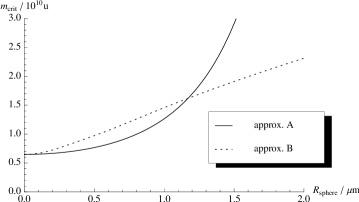
Figure 1: Critical mass for a hollow sphere as indicated by the behaviour of the second moment. We used a wave-packet width of $0.5\,\mu\mathrm{m}$.

In [22] we studied two simple models for the matter density $\rho_{c}$: a solid and a hollow sphere. The solid-sphere suffers from some peculiar divergence issues which we explain in B and is also mathematically slightly more difficult to handle than the hollow sphere whose radial mass distribution is just a $\delta$-function. We therefore use the hollow sphere as a model to compare the two approximation ansätze given above.

While in [12, 2, 13, 22] the expression “collapse mass” was used in a rather loosely defined manner, here we define as critical mass the mass value for which at $t=0$ the second order time derivative of the second moment $Q(t)=\int\rmd^{3}\mathrm{\mathbf{c}}\,|\mathrm{\mathbf{c}}|^{2}|\psi(t;\mathrm{\mathbf{c}})|^{2}$ vanishes, i. e. $\ddot{Q}(t=0)=0$. (Note that for a real-valued initial wave-packet the first order time derivative always vanishes.) For the one-particle Schrödinger-Newton equation and a Gaussian wave packet of $0.5\,\mu\mathrm{m}$ width this yields a critical mass of $6.5\times 10^{9}$ u which fits very well with the numerical results obtained in [13].

For the hollow sphere we then obtain the analytic expression

$$m_{\text{crit}}=\left(\sqrt{\frac{\pi}{2}}\,\frac{3\hbar^{2}}{G\,a\,f(R/a)}\right)^{1/3}\approx 5.153\times 10^{9}\,\mathrm{u}\,\left((a/\mu\mathrm{m})\times f\left(\frac{R}{a}\right)\right)^{-1/3}$$ (40)

for the critical mass. This expression is derived in A. The function $f$ is constantly 1 in case of the one-particle Schrödinger-Newton equation and shows an exponential dependence on $R$ in case of the wide wave-function approximation. In case of the Born-Oppenheimer approximation $f$ is a rather complicated function that can be found in the appendix.

The resulting critical mass for a width of the centre-of-mass wave-function of $0.5\,\mu\mathrm{m}$ is plotted as a function of the hollow-sphere radius in figure 1. The curve that the figure shows for the wide wave-function approximation coincides well with the results we obtained in the purely numerical analysis in [22]. For the Born-Oppenheimer-Type approximation the plot shows a radius dependence of the collapse mass that is almost linear. This is in agreement with the result by Diósi [15] who estimates the width of the ground state for a solid sphere to be proportional to $(R/M)^{3/4}$.

5.3 Narrow wave-functions in the Born-Oppenheimer scheme

With the Born-Oppenheimer-Type approximation scheme just derived we now possess a tool with which we can consider the opposite geometric situation than that in Case A, namely for widths of the centre-of-mass wave-function $\psi$ which are much smaller than the extensions (diameters of the support) of the matter distribution $\rho_{c}$, i. e., for well localised mass centres inside the bulk of matter.

Let us recall that in Newtonian gravitational physics the overall gravitational self-energy of a mass distribution $\widetilde{\rho}$ is given by

$$U_{\rm g}(\widetilde{\rho}):=-\frac{G}{2}\int\,\rmd^{3}\mathrm{\mathbf{x}}\int\,\rmd^{3}\mathrm{\mathbf{x}}^{\prime}\ \frac{\widetilde{\rho}(\mathrm{\mathbf{x}})\widetilde{\rho}(\mathrm{\mathbf{x}}^{\prime})}{\|\mathrm{\mathbf{x}}-\mathrm{\mathbf{x}}^{\prime}\|}\,.$$ (41)

If $\widetilde{\rho}=\rho+\rho^{\prime}$, we have by the simple quadratic dependence on $\widetilde{\rho}$

$$U_{\rm g}(\rho+\rho^{\prime}):=U_{\rm g}(\rho)+U_{\rm g}(\rho^{\prime})+I_{\rm g}(\rho,\rho^{\prime})\,,$$ (42)

where

$$I_{\rm g}(\rho,\rho^{\prime}):=-G\int\,\rmd^{3}\mathrm{\mathbf{x}}\int\,\rmd^{3}\mathrm{\mathbf{x}}^{\prime}\ \frac{\rho(\mathrm{\mathbf{x}})\rho^{\prime}(\mathrm{\mathbf{x}}^{\prime})}{\|\mathrm{\mathbf{x}}-\mathrm{\mathbf{x}}^{\prime}\|}\,.$$ (43)

represents the mutual gravitational interaction of the matter represented by $\rho$ with that represented by $\rho^{\prime}$. In the special case $\rho^{\prime}=T_{\mathrm{\mathbf{d}}}\rho$, where $T_{\mathrm{\mathbf{d}}}$ denotes the operation of translation by the vector $\mathrm{\mathbf{d}}$,

$$\bigl{(}T_{\mathrm{\mathbf{d}}}\rho\bigr{)}(\mathrm{\mathbf{x}}):=\rho(\mathrm{\mathbf{x}}-\mathrm{\mathbf{d}})\,,$$ (44)

we set

$$I_{\rho}(\mathrm{\mathbf{d}}):=I_{\rm g}(\rho,T_{\mathrm{\mathbf{d}}}\rho)\,.$$ (45)

It is immediate from (43) that $I_{\rho}:\mathbb{R}^{3}\rightarrow\mathbb{R}$ has a zero derivative at the origin $\mathrm{\mathbf{0}}\in\mathbb{R}^{3}$,

$$I^{\prime}_{\rho}(\mathrm{\mathbf{0}})=0\,,$$ (46)

and that it satisfies the following equivariance

$$I_{\rho}(R\mathrm{\mathbf{d}})=I_{\rho\circ R}(\mathrm{\mathbf{d}})$$ (47)

for any orthogonal $3\times 3$ matrix $R$. The latter implies the rather obvious result that the function $\mathrm{\mathbf{d}}\mapsto I_{\rho}(\mathrm{\mathbf{d}})$ is rotationally invariant if $\rho$ is a rotationally invariant distribution, i. e., the interaction energy depends only on the modulus of the shift, not its direction.

For example, given that $\rho$ is the matter density of a homogeneous sphere of radius $R$ and mass $M$,

$$\rho(\mathrm{\mathbf{x}})=\begin{cases}\frac{3M}{4\pi R^{3}}&\text{for}\ \|\mathrm{\mathbf{x}}\|\leq R\\ 0&\text{for}\ \|\mathrm{\mathbf{x}}\|>R\,,\end{cases}$$ (48)

the gravitational interaction energy is between two such identical distributions a distance $d:=\|\mathrm{\mathbf{d}}\|$ apart is

$$I_{\rho}(d)=-\frac{GM^{2}}{R}\times\begin{cases}\frac{6}{5}-2\left(\frac{d}{2R}\right)^{2}+\frac{3}{2}\left(\frac{d}{2R}\right)^{3}-\frac{1}{5}\left(\frac{d}{2R}\right)^{5}&\text{for}\ d\leq 2R\,,\\ \frac{R}{d}&\text{for}\ d\geq 2R\,.\end{cases}$$ (49)

The second line is obvious, whereas the first line follows, e. g., from specialising the more general formula (42) of [16] to equal radii ($R_{p}=R_{t}$) and making the appropriate redefinitions in order to translate their electrostatic to our gravitational case. This formula also appears in [24].

Using the definitions (43) and (45), we can rewrite the right-hand side of (5.2) as convolution of $|\psi|^{2}$ with $I_{\rho_{c}}$:

$$V_{\rm g}^{(B)}(t;\mathrm{\mathbf{c}})=\int\,\rmd^{3}\mathrm{\mathbf{c}}^{\prime}\,I_{\rho_{c}}(\mathrm{\mathbf{c}}-\mathrm{\mathbf{c}}^{\prime})\,|\psi(t;\mathrm{\mathbf{c}}^{\prime})|^{2}\,.$$ (50)

Since in equation (3) this potential is multiplied with $\psi(t,\mathrm{\mathbf{c}})$, we see that only those values of $I_{\rho_{c}}(\mathrm{\mathbf{c}}-\mathrm{\mathbf{c}}^{\prime})$ will contribute where $|\psi(t;\mathrm{\mathbf{c}}^{\prime})|^{2}\psi(t;\mathrm{\mathbf{c}})$ appreciably differs from zero. Hence if $\psi$ is concentrated in a region of diameter $D$ then we need to know $I_{\rho_{c}}(\mathrm{\mathbf{c}}-\mathrm{\mathbf{c}}^{\prime})$ only for $\|\mathrm{\mathbf{c}}-\mathrm{\mathbf{c}}^{\prime}\|<D$. Assuming $D$ to be small we expand $I_{\rho_{c}}$ in a Taylor series. Because of (46) there is no linear term, so that up to and including the quadratic terms we have (using that $|\psi(t;\mathrm{\mathbf{c}}^{\prime})|^{2}$ is normalised with respect to the measure $\rmd^{3}\mathrm{\mathbf{c}}^{\prime}$)

$$V_{\rm g}^{(B)}(t;\mathrm{\mathbf{c}})\approx I_{\rho_{c}}(\mathrm{\mathbf{0}})+\tfrac{1}{2}I^{\prime\prime}_{\rho_{c}}(\mathrm{\mathbf{0}})\cdot\Bigl{(}\mathrm{\mathbf{c}}\otimes\mathrm{\mathbf{c}}-2\,\mathrm{\mathbf{c}}\otimes\langle\mathrm{\mathbf{c}}\rangle+\langle\mathrm{\mathbf{c}}\otimes\mathrm{\mathbf{c}}\rangle\Bigr{)}\,.$$ (51)

Here $I^{\prime\prime}_{\rho_{c}}(\mathrm{\mathbf{0}})$ denotes the second derivative of the function $I_{\rho_{c}}:\mathbb{R}^{3}\rightarrow\mathbb{R}$ at $\mathrm{\mathbf{0}}\in\mathbb{R}$ (which is a symmetric bilinear form on $\mathbb{R}^{3}$) and $\langle\,\cdot\,\rangle$ denotes the expectation value with respect to $\psi$. We stress that the non-linearity in $\psi$ is now entirely encoded into this state dependence of the expectation values which appear in the potential. If, for simplicity, we only consider centre-of-mass motions in one dimension, the latter being coordinatised by $c\in\mathbb{R}$, then (51) simplifies to

$$V_{\rm g}^{(B)}(t;c) \,\approx\,I_{\rho_{c}}(0)+\tfrac{1}{2}I^{\prime\prime}_{\rho_{c}}(0)\Bigl{(}c^{2}-2c\,\langle c\rangle+\langle c^{2}\rangle\Bigr{)}$$ (52a)

$$\,=\,I_{\rho_{c}}(0)+\tfrac{1}{2}I^{\prime\prime}_{\rho_{c}}(0)\bigl{(}c-\langle c\rangle\bigr{)}^{2}+\tfrac{1}{2}I^{\prime\prime}_{\rho_{c}}(0)\bigl{(}\langle c^{2}\rangle-\langle c\rangle^{2}\bigr{)}\,.$$ (52b)

The first term, $I_{\rho_{c}}(0)$, just adds a constant to the potential which can be absorbed by adding $-(\mathrm{i}/\hbar)I_{\rho_{c}}(0)t$ to the phase $\psi$. The second term is the crucial one and has been shown in [23] to give rise to interesting and potentially observable for Gaussian states.

More precisely, consider a one-dimensional non-linear Schrödinger evolution of the form (1a) with $V_{\rm g}$ given by the second term in (52) and an additional external harmonic potential for the centre of mass, then we get the following non-linear Schrödinger-Newton equation for the centre-of-mass wave-function,

$$\mathrm{i}\hbar\partial_{t}\psi(t;c)=\left(-\frac{\hbar^{2}}{2M}\frac{\partial^{2}}{\partial c^{2}}+\tfrac{1}{2}M\omega^{2}_{c}c^{2}+\tfrac{1}{2}M\omega^{2}_{\rm SN}\bigl{(}c-\langle c\rangle\bigr{)}^{2}\right)\,\psi(t;c)\,,$$ (53)

where $\omega_{\rm SN}:=\sqrt{I_{\rho_{c}}^{\prime\prime}(0)/M}$ is called the Schrödinger-Newton frequency. This equation has been considered in [23], where the last term on the right-hand side of (52b) has been neglected for a priori no good reason. Note that $\langle c^{2}\rangle$ and $\langle c\rangle^{2}$ contain the wave function and hence are therefore not constant (in time). Now, in the context of [23] the consequences of interest were the evolution equations for the first and second moments in the canonical phase-space variables, and it shows that for them only spatial derivatives of the potential contribute. As a consequence, the term in question makes no difference. The relevant steps in the computation are displayed in C.

Based on the observation that equation (53) evolves Gaussian states into Gaussian states, it has then been shown that the covariance ellipse of the Gaussian state rotates at frequency $\omega_{q}:=\sqrt{\omega_{c}^{2}+\omega^{2}_{\rm SN}}$ whereas the centre of the ellipse orbits the origin in phase with frequency $\omega_{c}$. This asynchrony results from a difference between first- and second-moment evolution and is a genuine effect of self gravity. It has been suggested that it may be observable via the output spectra of optomechanical systems [23].

6 Conclusions and outlook

Although the many-particle Schrödinger-Newton equation (5) does not exactly separate into centre-of-mass and relative motion, we could show that for some well-motivated approximations such a separation is possible. As long as the extent of an object is negligible in comparison to the uncertainty in localisation of its centre of mass the one-particle equation (3) is a good model in both approximation schemes considered.

In the opposite case of a well localised object, i. e. one that has a narrow wave-function compared to its extent, the gravitational potential takes the form (52) which yields a closed system of equations for the first and second moments and therefore the effects described in [23]. The non-linear Schrödinger equation resulting from the potential (52) is also considered in [24], where it is used for comparison of Schrödinger-Newton dynamics with models of quantum state reduction and decoherence.

The modification (38) provides a valid correction of the one-particle Schrödinger-Newton equation for objects of finite but small radii. This equation was considered in [25] and studied numerically in [22]. It remains unclear for which ratio of the object’s extent to the width of the wave-function the Born-Oppenheimer-Type approximation (5.2) starts to be superior to the wide wave-function approximation. It may even be the better approximation throughout the whole range of possible object sizes and wave-functions since a Born-Oppenheimer like approximation is implicitly assumed also for the wide wave-function when the mass density is taken to be that of a solid object.

In passing we make the final technical remark that the analysis of the critical mass for the hollow sphere shows that this mass increases linearly with the radius $R$ of the sphere. Given a fixed mass, this implies that the width of the stationary solution increases like $R^{3/4}$, a relation already found by Diósi [15].

The interface between Quantum Mechanics and gravity theory remains one of the most interesting and profound challenges with hopefully revealing experimental consequences, which we are only beginning to explore. In this context one should also mention that non-linear one-particle Schrödinger equations are of course also considered for Einstein-Bose condensates, in which case inclusion of self gravity adds a Schrödinger-Newton term in addition to that non-linear term obtained from the effective potential within the Hartree-Fock approximation (Gross-Pitaevskii-Newton equation). Such equations are derivable for particle numbers $N\rightarrow\infty$ without further hypotheses and may open up the possibility to test self-gravity effects on large quantum systems. Recent experiments have demonstrated the high potential of atom interferometry on freely falling Einstein-Bose condensates [26] and it seems an interesting question whether this may be used to see self-gravity effects on such systems.

Appendix A Comparison of approximations for spherically symmetric mass distributions

For both the wide wave-function approximation (38) and the Born-Oppenheimer-Type approximation (5.2) one must solve integrals of the type

$$I(\mathrm{\mathbf{a}})=\int\rmd^{3}\mathrm{\mathbf{r}}\;\frac{\rho_{c}(\mathrm{\mathbf{r}})}{\|\mathrm{\mathbf{r}}-\mathrm{\mathbf{a}}\|}\,.$$ (54)

In a spherically symmetric situation these take the form

$$I(a) =\int_{0}^{\infty}r^{2}\,\rmd r\int_{-1}^{1}\rmd\cos\theta\int_{0}^{2\pi}\rmd\varphi\,\frac{\rho_{c}(r)}{\sqrt{r^{2}+a^{2}-2ra\cos\theta}}$$

$$=\frac{4\pi}{a}\int_{0}^{a}\rmd r\,r^{2}\,\rho_{c}(r)+4\pi\int_{a}^{\infty}\rmd r\,r\,\rho_{c}(r)\,,$$ (55)

where we write $a$ for the absolute value $|\mathrm{\mathbf{a}}|$, etc. If now we assume that $\rho_{c}$ is the mass density of a hollow sphere of radius $R$, i. e.

$$\rho_{c}(r)=\frac{M}{4\pi\,r^{2}}\,\delta(r-R)\,,$$ (56)

these integrals simplify to

$$I_{R}(a)=\begin{cases}\frac{M}{R}&\mbox{if }a<R\\ \frac{M}{a}&\mbox{if }a\geq R\end{cases}\,.$$ (57)

With this the wide wave-function approximation (38) results in

$$V_{\rm g}^{(A)}(t;c;R)=-GM\int\rmd^{3}\mathrm{\mathbf{c}}^{\prime}\,|\psi(t;\mathrm{\mathbf{c}}^{\prime})|^{2}\,I_{R}(\|\mathrm{\mathbf{c}}-\mathrm{\mathbf{c}}^{\prime}\|)\,.$$ (58)

On the other hand, the Born-Oppenheimer approximation (5.2) leads to

$$V_{\rm g}^{(B)}(t;c;R)=-G\int\rmd^{3}\mathrm{\mathbf{c}}^{\prime}\,|\psi(t;\mathrm{\mathbf{c}}^{\prime})|^{2}\int\rmd^{3}\mathrm{\mathbf{r}}^{\prime}\,\rho_{c}(\mathrm{\mathbf{r}}^{\prime})\,I_{R}(\|\mathrm{\mathbf{c}}-\mathrm{\mathbf{c}}^{\prime}-\mathrm{\mathbf{r}}^{\prime}\|)\,.$$ (59)

In order to be able to obtain an analytical result we consider the initial Gaussian wave packet

$$\psi(t=0;\mathrm{\mathbf{c}})=(\pi a^{2})^{-3/4}\,\exp\left(-\frac{c^{2}}{2a^{2}}\right)\,,$$ (60)

for which these potentials take the form

$$V_{A}^{0}(c;R) =-\frac{GM^{2}}{2}\Bigg{\{}\frac{a}{\sqrt{\pi}\,c\,R}\left[\exp\left(-\frac{(c+R)^{2}}{a^{2}}\right)-\exp\left(-\frac{(c-R)^{2}}{a^{2}}\right)\right]$$

$$\mathrel{\phantom{=}}+\frac{1}{c}\left[\mathrm{erf}\left(\frac{c+R}{a}\right)+\mathrm{erf}\left(\frac{c-R}{a}\right)\right]$$

$$\mathrel{\phantom{=}}+\frac{1}{R}\left[\mathrm{erf}\left(\frac{c+R}{a}\right)-\mathrm{erf}\left(\frac{c-R}{a}\right)\right]\Bigg{\}}$$ (61)

$$V_{B}^{0}(c;R) =-\frac{GM^{2}}{2}\Bigg{\{}\frac{a}{\sqrt{\pi}\,c}\left(\frac{1}{R}+\frac{8R}{3a^{2}}\right)\exp\left(-\frac{(c+2R)^{2}}{a^{2}}\right)$$

$$\mathrel{\phantom{=}}+\frac{a}{\sqrt{\pi}\,R}\left(\frac{1}{2c}-\frac{1}{4R}\right)\left[\exp\left(-\frac{(c+2R)^{2}}{a^{2}}\right)-\exp\left(-\frac{(c-2R)^{2}}{a^{2}}\right)\right]$$

$$\mathrel{\phantom{=}}+\frac{1}{c}\left[\mathrm{erf}\left(\frac{c+2R}{a}\right)+\mathrm{erf}\left(\frac{c-2R}{a}\right)\right]$$

$$\mathrel{\phantom{=}}+\frac{1}{R}\left(1-\frac{c}{4R}-\frac{a^{2}}{8cR}\right)\left[\mathrm{erf}\left(\frac{c+2R}{a}\right)-\mathrm{erf}\left(\frac{c-2R}{a}\right)\right]\Bigg{\}}\,.$$ (62)

Note that both potentials agree in the limits

$$\lim_{R\to 0}V_{A,B}^{0}(c;R)=-\frac{GM^{2}}{c}\,\mathrm{erf}\left(\frac{c}{a}\right)\quad\text{and}\quad\lim_{R\to\infty}V_{A,B}^{0}(c;R)=0\,.$$ (63)

As a measure to compare these potentials with each other and the one-particle Schrödinger-Newton equation  we use the second moment $Q(t)=\int\rmd^{3}\mathrm{\mathbf{c}}\,|\mathrm{\mathbf{c}}|^{2}|\psi(t;\mathrm{\mathbf{c}})|^{2}$. For a real wave packet its first order time derivative can be shown to vanish. Therefore the sign of the second order time derivative $\ddot{Q}$ at $t=0$ determines if a wave packet initially shrinks or increases in width. In general the second order time derivative is

$$\ddot{Q}(t)=\int\rmd^{3}\mathrm{\mathbf{c}}\left(\frac{2\hbar^{2}}{M^{2}}|\mathrm{\mathbf{\nabla}}\psi(t;\mathrm{\mathbf{c}})|^{2}+\frac{2}{M}V_{\rm g}(t;\mathrm{\mathbf{c}})\left(3\,|\psi(t;\mathrm{\mathbf{c}})|^{2}+\mathrm{\mathbf{c}}\cdot\mathrm{\mathbf{\nabla}}|\psi(t;\mathrm{\mathbf{c}})|^{2}\right)\right)$$ (64)

which for the spherically symmetric gaussian state (60) takes the form

$$\ddot{Q}(t=0) =\frac{3\hbar^{2}}{M^{2}a^{2}}+\frac{8}{\sqrt{\pi}\,M\,a^{5}}\int_{0}^{\infty}\rmd c\,\exp\left(-\frac{c^{2}}{a^{2}}\right)\,V^{0}(c)\,\left(3a^{2}c^{2}-2c^{4}\right)$$ (65)

$$=\frac{3\hbar^{2}}{M^{2}a^{2}}-\sqrt{\frac{2}{\pi}}\frac{G\,M}{a}\,f\left(\frac{R}{a}\right)\,.$$ (66)

The critical mass defined by $\ddot{Q}(t=0)=0$ is then given by

$$m_{\text{crit}}=\left(\sqrt{\frac{\pi}{2}}\,\frac{3\hbar^{2}}{G\,a\,f(R/a)}\right)^{1/3}\approx 5.153\times 10^{9}\,\mathrm{u}\,\left((a/\mu\mathrm{m})\times f\left(\frac{R}{a}\right)\right)^{-1/3}\,.$$ (67)

The function $f$ is $f\equiv 1$ for the one-particle Schrödinger-Newton equation. For the hollow sphere potential in the wide wave-function and Born-Oppenheimer-Type approximations, (A) and (A), respectively, this function can be calculated as

$$f_{A}\left(\frac{R}{a}\right) =\exp\left(-\frac{R^{2}}{2a^{2}}\right)$$ (68)

$$f_{B}\left(\frac{R}{a}\right) =\frac{2}{3}\sqrt{\frac{2}{\pi}}\exp\left(-\frac{4R^{2}}{a^{2}}\right)\frac{R}{a}\left(1-\left(\frac{2R}{a}\right)^{2}\right)$$

$$\mathrel{\phantom{=}}+\exp\left(-\frac{2R^{2}}{a^{2}}\right)\left(1-\mathrm{erf}\left(\sqrt{2}\frac{R}{a}\right)\right)\left(1+\frac{1}{3}\left(\frac{2R}{a}\right)^{4}\right)$$

$$\mathrel{\phantom{=}}+\frac{a^{2}}{2R^{2}}\left(\frac{1}{\sqrt{2}}\mathrm{erf}\left(2\frac{R}{a}\right)-\exp\left(-\frac{2R^{2}}{a^{2}}\right)\mathrm{erf}\left(\sqrt{2}\frac{R}{a}\right)\right)\,.$$ (69)

Appendix B Divergence of the solid-sphere potential in the wide wave-function approximation

Given a spherically symmetric situation the wide wave-function approximation (38) takes the form

$$V(c)=(|\psi|^{2}*\Phi)(c)=4\pi\;\int_{0}^{\infty}\rmd c^{\prime}\;c^{\prime 2}\,|\psi(c^{\prime})|^{2}\,\Phi(|c-c^{\prime}|)\,,$$ (70)

where for the potential $\Phi$ we want to consider the following three cases:

• Coulomb potential (i. e. the case of the Schrödinger-Newton equation (3)):

  $$\Phi_{c}(c)=-\frac{1}{c}\,,$$ (71)

• hollow sphere of radius $R$:

  $$\Phi_{h}(c)=\begin{cases}-\frac{1}{R}&\mbox{if }c<R\\ \Phi_{c}(c)&\mbox{if }c\geq R\end{cases}\,,$$ (72)

• solid sphere of radius $R$:

  $$\Phi_{s}(c)=\begin{cases}-\frac{3}{2R}+\frac{c^{2}}{2R^{3}}&\mbox{if }c<R\\ \Phi_{c}(c)&\mbox{if }c\geq R\end{cases}\,.$$ (73)

First we want to study the behaviour of $V_{0}=V(c=0)$ for a Gaussian wave packet $|\psi(c)|^{2}=\frac{1}{4\pi}\exp(-c^{2})$. For convenience we omit all pre-factors. Equation (70) then reads:

$$V_{0} =\int_{0}^{\infty}\rmd c\;c^{2}\,\exp(-c^{2})\,\Phi(c)$$ (74)

$$=\int_{0}^{R}\rmd c\;c^{2}\,\exp(-c^{2})\,\Phi(c)+\int_{R}^{\infty}\rmd c\;c^{2}\,\exp(-c^{2})\,\Phi_{c}(c)$$ (75)

$$=\int_{0}^{R}\rmd c\;c^{2}\,\exp(-c^{2})\,\Phi(c)-\frac{\exp(-R^{2})}{2}\,.$$ (76)

For the three different potentials one obtains

$$V_{0,c} =\int_{0}^{R}\rmd c\;c^{2}\,\exp(-c^{2})\,\Phi_{c}(c)-\frac{\exp(-R^{2})}{2}$$

$$=-\frac{1}{2}+\frac{\exp(-R^{2})}{2}-\frac{\exp(-R^{2})}{2}$$

$$=-\frac{1}{2}$$ (77)

$$V_{0,h} =\int_{0}^{R}\rmd c\;c^{2}\,\exp(-c^{2})\,\Phi_{h}(c)-\frac{\exp(-R^{2})}{2}$$

$$=\frac{\exp(-R^{2})}{2}-\frac{\sqrt{\pi}}{4R}\mathrm{erf}(R)-\frac{\exp(-R^{2})}{2}$$

$$=-\frac{\sqrt{\pi}}{4R}\mathrm{erf}(R)$$ (78)

$$V_{0,s} =\frac{3}{2}\int_{0}^{R}\rmd c\;c^{2}\,\exp(-c^{2})\,\Phi_{h}(c)$$

$$\mathrel{\phantom{=}}+\frac{1}{2R^{3}}\int_{0}^{R}\rmd c\;c^{4}\exp(-c^{2})-\frac{\exp(-R^{2})}{2}$$

$$=-\frac{3\sqrt{\pi}}{8R}\mathrm{erf}(R)-\frac{3}{8R^{2}}\exp(-R^{2})-\frac{3\sqrt{\pi}}{16R^{2}}\mathrm{erf}(R)$$ (79)

In the limit $R\to 0$ the function $\mathrm{erf}(R)/R$ converges to $2/\sqrt{\pi}$. Thus, (78) converges to $-1/2$ and yields the same value as one gets for $\Phi_{c}$. For (79) both the second and third term diverge but the sum of both terms converges and altogether $V_{0,s}$ also converges to the value of $-1/2$. So everything seems fine.

But now consider the behaviour of $V(c)$ in a small neighbourhood of $c=0$, i. e. $V_{\varepsilon}=V(c=\varepsilon)$. For the hollow sphere this changes nothing of course, since the potential is constant within radius $R$. The potentials $\Phi_{c}$ and $\Phi_{s}$ can be expanded around $\varepsilon=0$ and yield

$$\Phi_{c}(c+\varepsilon) =\Phi_{c}(c)+\varepsilon\,\frac{1}{c^{2}}+\mathcal{O}(\varepsilon^{2})$$ (80)

$$\Phi_{s}(c+\varepsilon) =\Phi_{s}(c)+\varepsilon\,\frac{c}{R^{3}}+\mathcal{O}(\varepsilon^{2})\,.$$ (81)

This gives the additional contributions

$$V_{\varepsilon,c} =V_{0,c}+\varepsilon\,\int_{0}^{R}\rmd c\;\exp(-c^{2})$$ (82)

$$=V_{0,c}+\varepsilon\,\frac{\sqrt{\pi}}{2}\,\mathrm{erf}(R)$$ (83)

$$V_{\varepsilon,s} =V_{0,s}+\frac{\varepsilon}{R^{3}}\,\int_{0}^{R}\rmd c\;c^{3}\,\exp(-c^{2})$$ (84)

$$=V_{0,s}-\varepsilon\,\frac{1+R^{2}}{2}\,\exp(-R^{2})+\frac{\varepsilon}{2R^{3}}$$ (85)

to the potentials. For the Coulomb potential everything is fine since $\mathrm{erf}(R)\to 0$ for $R\to 0$. Hence, both the Coulomb and the hollow sphere potential obtain no further contributions at this order and it can be easily checked that this also holds for all higher orders in $\varepsilon$.

For the solid sphere potential, however, things are not fine at all. Not only does the term proportional to $\exp(-R^{2})$ in the limit $R\to 0$ yield a contribution $-\varepsilon/2$ which already makes it differ from the Coulomb potential. The last term is even worse because it diverges in this limit. Therefore, we cannot take this model seriously for small radii of the solid sphere and we are better off taking the hollow sphere potential as a toy model for the density of a molecule.

Appendix C Evolution equations for first and second moments in the narrow wave-function limit

Here we will explicitly derive the self-contained system of evolution equations for the first and second moments given in [23]. It has been noted there that since this system is closed, Gaussian states will remain Gaussian under evolution. We will show that the difference of our equation (52) to equation (53) given in [23] has no influence on this set of equations.

For this we consider the Schrödinger equation

$$\mathrm{i}\dot{\psi}=\frac{p^{2}}{2M}\psi+H_{1}\psi\,,$$ (86)

where

$$H_{1} =\frac{k}{2}\mathrm{\mathbf{x^{2}}}-k_{\text{SN}}\mathrm{\mathbf{x}}\cdot\langle\mathrm{\mathbf{x}}\rangle+\alpha\langle\mathrm{\mathbf{x}}\rangle^{2}+\beta\langle\mathrm{\mathbf{x}}^{2}\rangle$$

$$p_{i} =-\mathrm{i}\partial_{i}$$

$$k =k_{\text{CM}}+k_{\text{SN}}=M\omega_{\text{CM}}^{2}+M\omega_{\text{SN}}^{2}\,.$$

In principle, in the case of equation (52) we have $\alpha=0$, $\beta=k_{\text{SN}}/2$, while in the case of equation (53) $\alpha=k_{\text{SN}}/2$, $\beta=0$. But note that

$$\partial_{i}\langle\mathrm{\mathbf{x}}\rangle_{j} =0$$ (87a)

$$\partial_{i}\langle\mathrm{\mathbf{x}}^{2}\rangle =0\,.$$ (87b)

Therefore, independent of the choice of $\alpha$ and $\beta$ the derivatives of $H_{1}$ are

$$\partial_{i}H_{1} =kx_{i}-k_{\text{SN}}\langle\mathrm{\mathbf{x}}\rangle_{i}$$ (88a)

$$\Delta H_{1} =3k\,.$$ (88b)

We will see that $H_{1}$ will enter into the evolution equations for the first and second moments only through these derivatives. Thus, for the different equations (52) and (53) we obtain the same evolution equations for the first and second moments, which are:

$$\partial_{t}\langle\mathrm{\mathbf{x}}\rangle_{i} =\int\rmd^{3}x\,x_{i}\left(\psi^{*}\dot{\psi}+\psi\dot{\psi}^{*}\right)=\frac{\mathrm{i}}{2M}\int\rmd^{3}x\,x_{i}\left(\psi^{*}\Delta\psi-\psi\Delta\psi^{*}\right)$$ (89a)

$$=\frac{\mathrm{i}}{2M}\int\rmd^{3}x\left(-(\partial_{j}\psi)\partial_{j}(x_{i}\psi^{*})+(\partial_{j}\psi^{*})\partial_{j}(x_{i}\psi)\right)$$ (89b)

$$=\frac{\mathrm{i}}{2M}\int\rmd^{3}x\left(-\psi^{*}\partial_{i}\psi+\psi\partial_{i}\psi^{*}\right)=\frac{1}{M}\int\rmd^{3}x\,{\psi^{*}(-\mathrm{i}\partial_{i})\psi}$$ (89c)

$$=\frac{\langle\mathrm{\mathbf{p}}\rangle_{i}}{M}$$ (89d)

$$\partial_{t}\langle\mathrm{\mathbf{p}}\rangle_{i} =-\mathrm{i}\int\rmd^{3}x\left(\dot{\psi}^{*}\partial_{i}\psi+\psi^{*}\partial_{i}\dot{\psi}\right)$$ (90a)

$$=\frac{1}{2M}\int\rmd^{3}x\left(-(\Delta\psi^{*})\partial_{i}\psi+\psi^{*}\partial_{i}\Delta\psi\right)-\langle\partial_{i}H_{1}\rangle$$ (90b)

$$=\frac{1}{2M}\int\rmd^{3}x\left((\partial_{j}\psi^{*})\partial_{i}\partial_{j}\psi+\psi^{*}\partial_{i}\Delta\psi\right)-\langle\partial_{i}H_{1}\rangle$$ (90c)

$$=\frac{1}{2M}\int\rmd^{3}x\left(-\psi^{*}\partial_{i}\Delta\psi+\psi^{*}\partial_{i}\Delta\psi\right)-\langle\partial_{i}H_{1}\rangle$$ (90d)

$$=-k\langle\mathrm{\mathbf{x}}\rangle_{i}+k_{\text{SN}}\langle\mathrm{\mathbf{x}}\rangle_{i}$$ (90e)

$$=-k_{\text{CM}}\langle\mathrm{\mathbf{x}}\rangle_{i}$$ (90f)

$$\partial_{t}\langle\mathrm{\mathbf{x}}^{2}\rangle =\int\rmd^{3}x\,\mathrm{\mathbf{x}}^{2}\left(\psi^{*}\dot{\psi}+\psi\dot{\psi}^{*}\right)=\frac{\mathrm{i}}{2M}\int\rmd^{3}x\,\mathrm{\mathbf{x}}^{2}\left(\psi^{*}\Delta\psi-\psi\Delta\psi^{*}\right)$$ (91a)

$$=\frac{\mathrm{i}}{2M}\int\rmd^{3}x\left(-(\partial_{j}\psi)\partial_{j}(x_{i}x_{i}\psi^{*})+(\partial_{j}\psi^{*})\partial_{j}(x_{i}x_{i}\psi)\right)$$ (91b)

$$=\frac{\mathrm{i}}{M}\int\rmd^{3}x\left(-x_{i}\psi^{*}\partial_{i}\psi+x_{i}\psi\partial_{i}\psi^{*}\right)$$ (91c)

$$=\frac{1}{M}\int\rmd^{3}x\left(\psi^{*}x_{i}(-\mathrm{i}\partial_{i})\psi+\psi^{*}(-\mathrm{i}\partial_{i})(x_{i}\psi)\right)$$ (91d)

$$=\frac{1}{M}\left(\langle\mathrm{\mathbf{x}}\cdot\mathrm{\mathbf{p}}\rangle+\langle\mathrm{\mathbf{p}}\cdot\mathrm{\mathbf{x}}\rangle\right)$$ (91e)

$$\partial_{t}\langle\mathrm{\mathbf{p}}^{2}\rangle =-\int\rmd^{3}x\left(\dot{\psi}^{*}\Delta\psi+\psi^{*}\Delta\dot{\psi}\right)=\frac{\mathrm{i}}{2M}\int\rmd^{3}x\left((\Delta\psi^{*})\Delta\psi-\psi^{*}\Delta\Delta\psi\right)$$

$$\hskip 140.00021pt+2\mathrm{i}\int\rmd^{3}x\,\psi^{*}(\partial_{i}H_{1})\partial_{i}\psi+\mathrm{i}\langle\Delta H_{1}\rangle$$ (92a)

$$=2\mathrm{i}\int\rmd^{3}x\,\psi^{*}\left(kx_{i}-k_{\text{SN}}\langle\mathrm{\mathbf{x}}\rangle_{i}\right)\partial_{i}\psi+3\mathrm{i}k$$ (92b)

$$=-2k\int\rmd^{3}x\,\psi^{*}x_{i}(-\mathrm{i}\partial_{i})\psi+2k_{\text{SN}}\langle\mathrm{\mathbf{x}}\rangle_{i}\int\rmd^{3}x\,\psi^{*}(-\mathrm{i}\partial_{i})\psi+3\mathrm{i}k$$ (92c)

$$=-2k\langle\mathrm{\mathbf{x}}\cdot\mathrm{\mathbf{p}}\rangle+2k_{\text{SN}}\langle\mathrm{\mathbf{x}}\rangle\cdot\langle\mathrm{\mathbf{p}}\rangle+k\langle\mathrm{\mathbf{x}}\cdot\mathrm{\mathbf{p}}\rangle-k\langle\mathrm{\mathbf{p}}\cdot\mathrm{\mathbf{x}}\rangle$$ (92d)

$$=-k\left(\langle\mathrm{\mathbf{x}}\cdot\mathrm{\mathbf{p}}\rangle+\langle\mathrm{\mathbf{p}}\cdot\mathrm{\mathbf{x}}\rangle\right)+2k_{\text{SN}}\langle\mathrm{\mathbf{x}}\rangle\cdot\langle\mathrm{\mathbf{p}}\rangle$$ (92e)

$$\partial_{t}\langle\mathrm{\mathbf{x}}\cdot\mathrm{\mathbf{p}}\rangle =\partial_{t}\langle\mathrm{\mathbf{p}}\cdot\mathrm{\mathbf{x}}\rangle=\int\rmd^{3}x\left(\dot{\psi}^{*}x_{i}(-\mathrm{i}\partial_{i})\psi+\psi^{*}x_{i}(-\mathrm{i}\partial_{i})\dot{\psi}\right)$$ (93a)

$$=-\frac{1}{2M}\int\rmd^{3}x\,x_{i}\left((\Delta\psi^{*})\partial_{i}\psi-\psi^{*}\partial_{i}\Delta\psi\right)-\langle x_{i}\partial_{i}H_{1}\rangle$$ (93b)

$$=\frac{1}{2M}\int\rmd^{3}x\,(\partial_{j}\psi^{*})\partial_{j}(x_{i}\partial_{i}\psi)+\frac{1}{2M}\int\rmd^{3}x\,x_{i}\psi^{*}\partial_{i}\Delta\psi-\langle x_{i}\partial_{i}H_{1}\rangle$$ (93c)

$$=\frac{1}{2M}\int\rmd^{3}x\left((\partial_{i}\psi^{*})\partial_{i}\psi+x_{i}(\partial_{j}\psi^{*})\partial_{i}\partial_{j}\psi+x_{i}\psi^{*}\partial_{i}\Delta\psi\right)-\langle x_{i}\partial_{i}H_{1}\rangle$$ (93d)

$$=\frac{1}{2M}\int\rmd^{3}x\left(-\psi^{*}\Delta\psi-\psi^{*}\partial_{j}(x_{i}\partial_{i}\partial_{j}\psi)+x_{i}\psi^{*}\partial_{i}\Delta\psi\right)-\langle x_{i}\partial_{i}H_{1}\rangle$$ (93e)

$$=-\frac{1}{M}\int\rmd^{3}x\,\psi^{*}\Delta\psi-\langle x_{i}\partial_{i}H_{1}\rangle$$ (93f)

$$=\frac{\langle\mathrm{\mathbf{p}}^{2}\rangle}{M}-k\langle\mathrm{\mathbf{x}}^{2}\rangle+k_{\text{SN}}\langle\mathrm{\mathbf{x}}\rangle^{2}$$ (93g)

The same evolution equations are obtained by operators $\mathrm{\mathbf{x}}$ and $\mathrm{\mathbf{p}}$ that in the Heisenberg picture fulfil

$$\partial_{t}\mathrm{\mathbf{x}} =\frac{\mathrm{\mathbf{p}}}{M}$$ (94a)

$$\partial_{t}\mathrm{\mathbf{p}} =-k_{\text{CM}}\mathrm{\mathbf{x}}-k_{\text{SN}}(\mathrm{\mathbf{x}}-\langle\mathrm{\mathbf{x}}\rangle)\,.$$ (94b)

This was used in [23] to describe the effect of the Schrödinger-Newton equation on Gaussian states.

References

References

• [1] Rosenfeld L 1963 Nuclear Physics 40 353–356
• [2] Carlip S 2008 Classical and Quantum Gravity 25 154010 (6 pages)
• [3] Giulini D and Großardt A 2012 Classical and Quantum Gravity 29 215010 (25 pages)
• [4] Wald R M 1994 Quantum Field Theory in Curved Spacetime and Black Hole Thermodynamics Chicago Lectures in Physics (Chicago: The University of Chicago Press)
• [5] Anastopoulos C and Hu B L 2014 Problems with the Newton-Schrödinger equations arXiv:1403.4921
• [6] Anastopoulos C and Hu B L 2014 Newton-Schrödinger equations are not derivable from General Relativity + Quantum Field Theory arXiv:1402.3813
• [7] Page D N and Geilker C 1981 Physical Review Letters 47 979–982
• [8] Eppely K and Hannah E 1977 Foundations of Physics 7 51–68
• [9] Mattingly J 2005 Is quantum gravity necessary? Einstein Studies Volume 11. The Universe of General Relativity Einstein Studies ed Kox A J and Eisenstaedt J (Boston: Birkhäuser) chap 17, pp 327–338
• [10] Mattingly J 2006 Physical Review D 73 064025 (8 pages)
• [11] Albers M, Kiefer C and Reginatto M 2008 Physical Review D 78 064051 (17 pages)
• [12] Salzman P J and Carlip S A possible experimental test of quantized gravity arXiv:gr-qc/0606120 based on the Ph.D. thesis of P. Salzman: “Investigation of the Time Dependent Schrödinger-Newton Equation”, Univ. of California at Davis, 2005
• [13] Giulini D and Großardt A 2011 Classical and Quantum Gravity 28 195026 (17 pages)
• [14] Hornberger K, Gerlich S, Haslinger P, Nimmrichter S and Arndt M 2012 Reviews of Modern Physics 84 157–173
• [15] Diósi L 1984 Physics Letters A 105 199–202
• [16] Iwe H 182 Zeitschrift für Physik A: Atoms and Nuclei 304 347–361
• [17] Grawert G 1977 Quantenmechanik 3rd ed (Wiesbaden, Germany: Akademische Verlagsgesellschaft)
• [18] Heisenberg W 1949 The Physical Principles of the Quantum Theory (Mineola, New York: Dover Publications). Lectures delivered 1929 at the Univerity of Chicago
• [19] Christian J 1997 Physical Review D 56 4844–4877
• [20] Adler S L 2007 Journal of Physics A: Mathematical and Theoretical 40 755–763
• [21] Schrödinger E 1927 Annalen der Physik (Vierte Folge) 82 265–272
• [22] Giulini D and Großardt A 2013 Classical and Quantum Gravity 30 155018 (9 pages)
• [23] Yang H, Miao H, Lee D S, Helou B and Chen Y 2013 Physical Review Letters 110 170401 (5 pages)
• [24] Colin S, Durt T and Willox R 2014 Crucial tests of macrorealist and semi-classical gravity models with freely falling mesoscopic nanospheres arXiv:1402.5653 [quant-ph]
• [25] Jääskeläinen M 2012 Physical Review A 86 052105 (5 pages)
• [26] Müntinga H, Ahlers H, Krutzik M, Wenzlawski A, Arnold S, Becker D, Bongs K, Dittus H, Duncker H, Gaaloul N, Gherasim C, Giese E, Grzeschik C, Hänsch T W, Hellmig O, Herr W, Herrmann S, Kajari E, Kleinert S, Lämmerzahl C, Lewoczko-Adamczyk W, Malcolm J, Meyer N, Nolte R, Peters A, Popp M, Reichel J, Roura A, Rudolph J, Schiemangk M, Schneider M, Seidel S T, Sengstock K, Tamma V, Valenzuela T, Vogel A, Walser R, Wendrich T, Windpassinger P, Zeller W, van Zoest T, Ertmer W, Schleich W P and Rasel E M 2013 Physical Review Letters 110 093602 (5 pages)