Random local attraction driven metal-superconductor transitions

Abstract

In this paper, we investigate the disordered attractive Hubbard model by combining dynamical mean field theory, coherent potential approximation and iterated perturbation theory for superconductivity as an impurity solver. Disorder is introduced in the local attraction $U$. We assume that $U$ is distributed according to a bimodal probability distribution, wherein an $x$ fraction of sites are pairing centers ($U\neq 0$) and $(1-x)$ fraction of sites are non-interacting ($U=0$). It is found that beyond a critical $x=x_{c}$, a first order metal-superconductor phase transition leads to superconductivity being induced in the interacting as well as non-interacting sites.

1 Introduction

The combined effect of disorder and correlations on the superconducting state has been extensively studied since many decades but a complete picture has not emerged yet [1, 2]. A scenario of randomly located pairing centers leading to $s$-wave superconductivity may not be far-fetched and might be appropriate for real systems such as Tl-doped PbTe. The semiconducting PbTe, when doped with Tl (Pb_1-xTl_xTe), exhibits a superconducting ground state [3, 4] beyond a critical concentration ($x=x_{c}=0.3\%$) of Tl. The consensus regarding the origin of such doping induced superconductivity is that the Tl dopants represent spatially inhomogeneous centers of negative attractive interactions ($-U$), which nucleate Cooper pairing, and hence lead to superconductivity [5]. It was found  [3, 4] that the transition temperature, $T_{c}$, increases with increasing $x$ thus supporting the idea that Tl-dopants nucleate superconductivity.

A spatial distribution of attractive interaction centers may be mathematically represented by the attractive Hubbard model (AHM), with random attractive Hubbard interactions. We use the framework of dynamical mean field theory (DMFT) [6, 7, 8] combined with coherent potential approximation (CPA) [9, 10] to investigate this model. We employ two impurity solvers within DMFT: iterated perturbation theory for superconducting case (IPTSC) [11] and static mean-field theory [12, 13]. The random interaction is taken to be distributed according to a bimodal probability distribution. While $x$ fraction of sites have an attractive interaction, $-U$, $1-x$ fraction of sites are non-interacting. It is observed that beyond a critical $x=x_{c}$ the system is superconducting, but for large $U$ values, a small value of $x$ is sufficient to make whole system superconducting. The clean limit of the AHM has been extensively studied using Bogoliubov-de Gennes type mean field (BdGMF) theories and more recently using iterated perturbation theory with superconducting bath (IPTSC) [11, 14, 15], numerical renormalization group (NRG) [16] and continuous time quantum Monte Carlo (CTQMC) [17] within DMFT. The main issue that has been focused upon is the BCS-BEC crossover for different fillings and interaction strengths. The IPTSC method is known to benchmark excellently when compared to results from numerical renormalization group for the bulk AHM [16]. In this paper, we carry out a detailed study of the AHM with inhomogeneous interaction by combining CPA with DMFT and iterated perturbation theory for superconductivity(IPTSC). To distinguish between dynamical and static effects, we have also carried out BdGMF studies within CPA+DMFT. This paper is structured as follows: In the following section, we outline the model and the formalism used. Next, we present our results for the local order parameter, spectra and disorder induced phase transitions. We conclude in the final section.

2 Model and Method

We consider the single band attractive Hubbard model(AHM), which is given by the following Hamiltonian,

$${\cal H}=\sum_{i\sigma}\epsilon c^{\dagger}_{i\sigma}c^{\phantom{\dagger}}_{i\sigma}-t\sum_{\langle ij\sigma\rangle}\left(c^{\dagger}_{i\sigma}c^{\phantom{\dagger}}_{j\sigma}+h.c\right)-$$

$$\sum_{i}|U_{i}|\left(n_{i\uparrow}-\frac{1}{2}\right)\left(n_{i\downarrow}-\frac{1}{2}\right)-\mu\sum_{i\sigma}c^{\dagger}_{i\sigma}c^{\phantom{\dagger}}_{i\sigma}$$ (1)

Where ${c}_{i\sigma}$ annihilates an electron on $i^{\rm th}$ lattice site with spin $\sigma$, and ${n}_{i\sigma}=c^{\dagger}_{i\sigma}c^{\phantom{{\dagger}}}_{i\sigma}$, t is nearest neighbour hopping matrix, ${\epsilon}$ is onsite energy, and $\mu$ is chemical potential. The local disorder is given by random attractive Hubbard interaction, which is distributed according to the bimodal probability distribution function $P_{U}(U_{i})$

$${P_{U}(U_{i})}=(1-x)\delta(U_{i})+x\delta(U_{i}+U)\,,$$ (2)

where $1-x$ and $x$ are fractions of lattice sites with interaction $U_{i}=0$ and $U_{i}=-U$, respectively. Within DMFT, the lattice model is mapped onto a single-impurity model embedded in a self-consistently determined bath. For the present problem, the effective medium is in a superconducting state, hence the Nambu formalism must be used. The effective action [6, 18] for a given site $i$ within DMFT in Nambu formalism is given by

$$\hat{S}_{eff}(i)=-\int_{0}^{\beta}\ d\tau_{1}\int_{0}^{\beta}\ d\tau_{2}\Psi^{\dagger}_{i}(\tau_{1})\hat{\cal G}^{-1}(\tau_{1}-\tau_{2})\Psi_{i}(\tau_{2})-$$

$$|U_{i}|\int_{0}^{\beta}d\tau n_{i\uparrow}(\tau)n_{i\downarrow}(\tau)$$

where $\Psi_{i}(\tau)$, the two component Nambu’s spinor and $\hat{\cal G}(\tau)$, the host Green’s function in Nambu formalism are given by

$$\Psi_{i}(\tau)=\left[\begin{array}[]{ll}{c_{i\uparrow}(\tau)}\\ {c^{\dagger}_{i\downarrow}}(\tau)\end{array}\right]$$

and

$${\hat{\cal G}}(\omega)=\left[\begin{array}[]{ll}{\omega^{+}-\epsilon+\mu-\Delta_{11}(\omega)}&{-\Delta_{12}(\omega)}\\ {-\Delta_{21}(\omega)}&{\omega^{+}+\epsilon-\mu-\Delta_{22}(\omega)}\end{array}\right]^{-1}$$

Where ${\omega}^{+}={\omega}+i\eta$, and $\eta\rightarrow 0^{+}$. The impurity Green’s function in Nambu formalism is given as

$$\hat{G}^{i}(\tau)=-\langle T_{\tau}\Psi_{i}(\tau)\Psi^{\dagger}_{i}(0)\rangle$$

To discuss how disorder affects superconductivity, we use CPA with DMFT. The impurity Green’s function in Nambu formalism is given as

$${\hat{G}^{i}}(\omega)=\left[\begin{array}[]{ll}{\xi_{11}({\omega})-\Sigma_{i}(\omega)}&{-\Delta_{12}(\omega)-S_{i}(\omega)}\\ {-\Delta_{21}(\omega)-S_{i}(\omega)}&{\xi_{22}({\omega})+\Sigma^{*}_{i}(-\omega)}\end{array}\right]^{-1}$$ (6)

where, $\xi_{11}({\omega})=\omega^{+}+\mu-\epsilon-\Delta_{11}(\omega)$,  $\xi_{22}({\omega})=\omega^{+}-\mu+\epsilon-\Delta_{22}(\omega)$, $\Delta_{11}({\omega}),\ \Delta_{12}({\omega}),\ \Delta_{21}({\omega})$ and $\Delta_{22}({\omega})$ are components of the hybridisation function matrix $\hat{\Delta}({\omega})$, and $\Sigma_{i}({\omega})$ and $S_{i}({\omega})$ are normal and anomalous self-energies respectively. Now, by doing an arithmetic averaging over Hubbard interaction, the average local Green’s function is given as

$$\hat{G}^{CPA}(\omega)=\int d{U_{i}}\hat{G_{i}}(\omega)P_{U}({U_{i}})$$ (7)

From equations (2, 6, and 7) $\hat{G}^{CPA}(\omega)$ is given by:,

$$\hat{G}^{CPA}(\omega)=(1-x)\hat{G}^{0}(\omega)+x\hat{G}^{U}(\omega)$$ (8)

where $\hat{G}^{0}(\omega)$ and $\hat{G}^{U}(\omega)$ are given by

$${\hat{G}^{0}}(\omega)=\left[\begin{array}[]{ll}{\omega^{+}+\mu-\epsilon-\Delta_{11}(\omega)}&{-\Delta_{12}(\omega)}\\ {-\Delta_{21}(\omega)}&{\omega^{+}-\mu+\epsilon-\Delta_{22}(\omega)}\end{array}\right]^{-1}$$ (9)

$${\hat{G}^{U}}(\omega)=\left[\begin{array}[]{ll}{\xi_{11}(\omega)-\Sigma(\omega)}&{-\Delta_{12}(\omega)-S(\omega)}\\ {-\Delta_{21}(\omega)-S(\omega)}&{\xi_{22}(\omega)+\Sigma^{*}(-\omega)}\end{array}\right]^{-1}$$ (12)

To calculate $\Sigma(\omega)$ and $S(\omega)$ we employ IPTSC [11] as an impurity solver. These self-energies are given by:

$$\Sigma(\omega)=-U\frac{n}{2}+A\Sigma^{(2)}(\omega)$$ (13)

$$S(\omega)=-U\Phi+AS^{(2)}(\omega)$$ (14)

$$\Sigma^{(2)}(\omega)=U^{2}\int_{-\infty}^{\infty}\prod_{i=1}^{3}d\epsilon_{i}\frac{g_{1}(\epsilon_{1},\epsilon_{2},\epsilon_{3})N(\epsilon_{1},\epsilon_{2},\epsilon_{3})}{\omega^{+}-\epsilon_{1}+\epsilon_{2}-\epsilon_{3}}$$ (15)

$$S^{(2)}(\omega)=U^{2}\int_{-\infty}^{\infty}\prod_{i=1}^{3}d\epsilon_{i}\frac{g_{2}(\epsilon_{1},\epsilon_{2},\epsilon_{3})N(\epsilon_{1},\epsilon_{2},\epsilon_{3})}{\omega^{+}-\epsilon_{1}+\epsilon_{2}-\epsilon_{3}}$$ (16)

$${\hat{\cal{G}}^{U}}(\omega)=\left[\begin{array}[]{ll}{\xi_{11}({\omega})+U\frac{n}{2}}&{-\Delta_{12}(\omega)+U\Phi}\\ {-\Delta_{21}(\omega)+U\Phi}&\xi_{22}({\omega})-U\frac{n}{2}\end{array}\right]^{-1}$$ (19)

$$-\rm{Im}\frac{\hat{\cal{G}}^{U}(\omega)}{\pi}=\left[\begin{array}[]{ll}{\tilde{\rho}_{11}(\omega)}&{\tilde{\rho}_{12}(\omega)}\\ {\tilde{\rho}_{21}(\omega)}&{\tilde{\rho}_{22}(\omega)}\end{array}\right]$$ (20)

$$N(\epsilon_{1},\epsilon_{2},\epsilon_{3})=f(\epsilon_{1})f(-\epsilon_{2})f(\epsilon_{3})+f(-\epsilon_{1})f(\epsilon_{2})f(-\epsilon_{3})$$ (21)

$$g_{1}(\epsilon_{1},\epsilon_{2},\epsilon_{3})=\tilde{\rho}_{11}(\epsilon_{1})\tilde{\rho}_{22}(\epsilon_{2})\tilde{\rho}_{22}(\epsilon_{3})-\tilde{\rho}_{12}(\epsilon_{1})\tilde{\rho}_{22}(\epsilon_{2})\tilde{\rho}_{12}(\epsilon_{3})$$ (22)

$$g_{2}(\epsilon_{1},\epsilon_{2},\epsilon_{3})=\tilde{\rho}_{12}(\epsilon_{1})\tilde{\rho}_{12}(\epsilon_{2})\tilde{\rho}_{12}(\epsilon_{3})-\tilde{\rho}_{11}(\epsilon_{1})\tilde{\rho}_{12}(\epsilon_{2})\tilde{\rho}_{22}(\epsilon_{3})$$ (23)

$$A=\frac{\frac{n}{2}(1-\frac{n}{2})-\Phi^{2}}{{\frac{n_{0}}{2}(1-\frac{n_{0}}{2})-\Phi_{0}^{2}}}$$ (24)

where $\Phi$, $\Phi_{0}$, $n$ and $n_{0}$ are given by :,

$$\Phi=\int_{-\infty}^{\infty}d\omega\frac{-{\rm{Im}(G^{U}_{12}}(\omega))}{\pi}f(\omega)$$ (25)

$$\Phi_{0}=\int_{-\infty}^{\infty}d\omega\tilde{\rho}_{12}(\omega)f(\omega)$$ (26)

$$n=2\int_{-\infty}^{\infty}d\omega\frac{-{\rm{Im}(G^{U}_{11}}(\omega))}{\pi}f(\omega)$$ (27)

$$n_{0}=2\int_{-\infty}^{\infty}d\omega\tilde{\rho}_{11}(\omega)f(\omega)$$ (28)

The CPA Green’s function in term of average self-energy is given by

$$\hat{G}^{CPA}(\omega)=\left[\begin{array}[]{ll}{\xi_{11}(\omega)-\Sigma_{11}^{CPA}(\omega)}&{-\Delta_{12}(\omega)-\Sigma_{12}^{CPA}(\omega)}\\ {-\Delta_{21}(\omega)-\Sigma_{21}^{CPA}(\omega)}&\xi_{22}(\omega)-\Sigma_{22}^{CPA}(\omega)\end{array}\right]^{-1}$$ (31)

The lattice Green’s function is given by:

$$\hat{G}{(\vec{k},\omega)}=\left[\begin{array}[]{ll}{\bar{\omega}_{1}-\epsilon{(\vec{k})}}&{-\Sigma_{12}^{CPA}(\omega)}\\ {-\Sigma_{21}^{CPA}(\omega)}&{\bar{\omega}_{2}+\epsilon{(\vec{k})}}\end{array}\right]^{-1}$$ (34)

where $\bar{\omega}_{1}=\omega^{+}-\epsilon+\mu-\Sigma_{11}^{CPA}(\omega)$ and $\bar{\omega}_{2}=\omega^{+}+\epsilon-\mu-\Sigma_{22}^{CPA}(\omega)$. Finally, the CPA self-consistency is achieved by equating the local Green’s function to average impurity Green’s function :,

$$\frac{1}{N_{s}}\sum_{\vec{k}}\hat{G}{(\vec{k},\omega)}=\hat{G}^{CPA}(\omega)$$

$$\hat{G}^{CPA}(\omega)=\int^{\infty}_{-\infty}d\epsilon\rho_{0}(\epsilon)\hat{G}{(\epsilon,\omega)}$$ (35)

Where, $N_{s}$ is the number of lattice sites and $\rho_{0}(\epsilon)$ is the non-interacting density of states. We have used a semi-elliptic $\rho_{0}(\epsilon)$, given by $\rho_{0}(\epsilon)=2/\pi\sqrt{(1-\epsilon^{2})}$, $\epsilon\in[-1,1]$.

3 Numerical Algorithm

In practice, we follow the steps outlined below to obtain the converged order parameter and spectra.

1. Guess a hybridization matrix $\hat{\Delta}(\omega)$ for interacting and non-interacting site and $n,\Phi$ for interacting sites. In practice, we choose either a previously converged solution or the non-interacting $\hat{\Delta}(\omega)$ with $n=1$ and $\Phi=1/2$.

2. Given a hybridization, occupancy and order parameter, use equation (19) to calculate the host Green’s function matrix ${\hat{\cal{G}}}^{U}(\omega)$.

3. From equations (28 and 26), calculate pseudo-occupancy and pseudo-order parameter $n_{0}$ and $\Phi_{0}$.

4. Now, by using equations (13, 14, 15, 16, and 24), calculate the regular and anomalous self-energies $\Sigma(\omega)$ and $S(\omega)$.

5. Then, by using equations (9, 12, 13 and 14 ), calculate impurity Green’s function $\hat{G}^{0}(\omega)$, $\hat{G}^{U}(\omega)$, $n$ and $\Phi$ .

6. The disorder-averaged Green’s function, $\hat{G}^{\scriptscriptstyle CPA}(\omega)$ is obtained using equation (8).

7. We consider the AHM on Bethe lattice of infinite connectivity at half filling, which is achieved by setting $\mu=0,\epsilon=0$. For Bethe lattice the self-consistency condition is simply given by :,

   $$\hat{\Delta}(\omega)=\frac{t^{2}\sigma_{z}\hat{G}^{\scriptscriptstyle CPA}(\omega)\sigma_{z}}{4}$$ (36)

   where $\sigma_{z}$ is z component of Pauli’s matrix. Using equation (36), a new hybridization matrix $\hat{\Delta}({\omega})$ is obtained.

8. If the hybridization matrix $\hat{\Delta}(\omega)$ from step 7 and $n,\Phi$ from step 5 are equal (within a desired numerical tolerance) to the guess hybridization matrix $\hat{\Delta}(\omega)$, $n$ and $\Phi$ from step 1, then the iterations may be stopped, else the iterations continue until the desired convergence is achieved.

The results obtained using the above-mentioned procedure will be denoted as IPTSC. We have also carried out mean-field calculations by ‘turning off’ the dynamical self-energies in equations 13 and 14. These results will be denoted as BdGMF.

4 Results and Discussion

In this paper, we have considered $1-x$ fraction of the sites to be non-interacting ($U=0$), and $x$ fraction to be interacting ($U\neq 0$). The unit of energy is the hopping integral $t=1$. We have done all the calculations at half filling ($\langle n\rangle=1$), which is fixed by taking $\mu=\epsilon=0$.

4.1 Spectral functions

In figure 1, the 11 and 12 components of local spectral functions as a function of frequency are shown for different values of $x$ at $U=1.5$. The panel (a) and (b) represent the 11 and 12 components of spectral function of interacting site respectively. $\rho^{U}_{11}(\omega)$, $\rho^{U}_{12}(\omega)$, $\rho^{0}_{11}(\omega)$, and $\rho^{0}_{12}(\omega)$ represent the 11 and 12 components of local spectral function of the interacting and non-interacting sites respectively. For a $U=1.5$, we find that, beyond a critical value of $x\sim 0.70$ the $\rho^{U}_{11}(\omega)$ becomes gapped, and the gap increases with increasing $x$. The spectral function has coherence peaks at the gap edges, and the weight of the coherence peak increases with increasing $x$. Concomitantly, beyond $x\sim 0.70$, the off-diagonal spectrum, $\rho^{U}_{12}(\omega)$ develops finite spectral weight, which increases with increasing $x$. This also implies that the local superconducting order parameter, $\Phi$, given by integration of $\rho^{U}_{12}(\omega)$ upto the Fermi level, increases with increasing $x$. Thus we conclude that the spectral gap of figure 1(a) is superconducting in nature. We find that the non-interacting sites also develop superconductivity. This is seen from the evolution of the local spectral functions corresponding to the non-interacting sites, which are shown in the two lower panel of figure 1. This is natural because the host in which the interacting and non-interacting sites are embedded, characterized by $\hat{\Delta}({\omega})$, becomes superconducting.

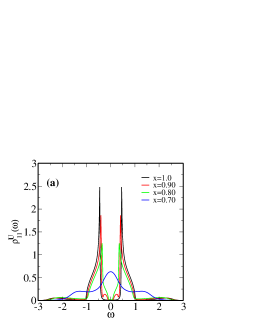
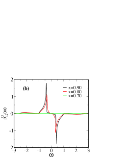
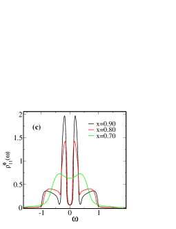
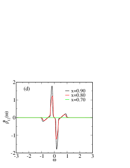
Figure 1: Diagonal (a,c) and off-diagonal (b,d) spectral function as a function of frequency for interacting and non-interacting site respectively at U=1.5.

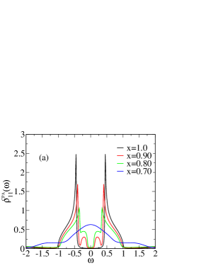
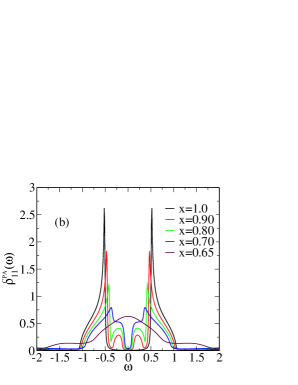
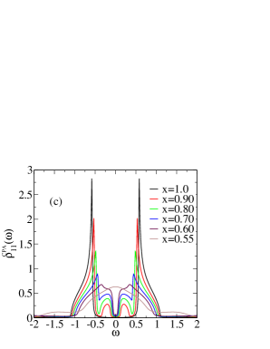
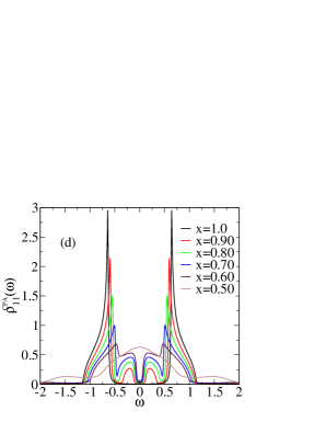
Figure 2: Diagonal component of CPA spectral function as a function of frequency for (a) U=1.5 (b) U=1.6 (c) U=1.7 (d) U=1.8.

In figure 2 the 11 component of disorder averaged spectral function is shown for various values of $x$ computed with $U=1.5,1.6,1.7$ and, $1.8$. It is seen all the spectra are gapped at $x=1.0$. With increasing $x$, the gap increases, and finally a metal to superconductor transition occurs at a critical $x_{c}$. The nature of this transition and the dependence of $x_{c}$ on $U$ will be discussed next.

4.2 Metal-superconductor transition

The results in the previous sections suggest the following scenario: For $x=0$, there are no sites with $-U$, and the system is a metal. With increasing $x$, the system develops superconductivity beyond a critical $x_{c}$. The disorder averaged superconducting order parameter $(\Phi^{CPA})$, calculated by using the expression,

$$\Phi^{CPA}=\int_{-\infty}^{\infty}d\omega\frac{-\rm{Im}(G^{CPA}_{12}(\omega))f(\omega)}{\pi}\,,$$ (37)

is shown in upper panel of figure 3 as a function of $x$ for different values of $U$.

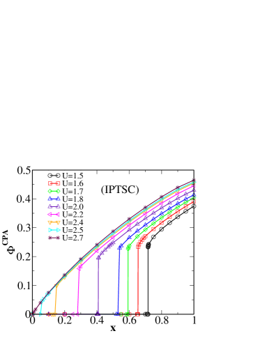
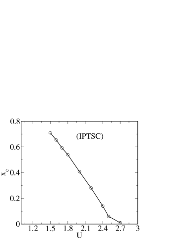
Figure 3: Upper panel: Disorder averaged superconducting order $(\Phi^{CPA})$ as a function of $x$ for different values of $U$. Lower Panel : The critical fraction of interacting sites, $x_{c}$ vs $U$.

For all $U\lesssim 2.7$, a finite $x_{c}$ is needed before the superconducting order develops. The transition from metal to superconductor is seen to be first order. The critical $x_{c}$ decreases sharply with increasing $U$ as seen in the lower panel. For all $U\geqslant 2.7$, the transition becomes continuous and the critical $x_{c}$ needed to generate superconductivity is nearly zero. This indicates that the interaction stabilises the superconducting phase despite the presence of disorder. The $x_{c}\rightarrow 0$ for $U\gtrsim 2.7$ is most likely an artefact of the infinite coordination number within dynamical mean field theory. Including non-local dynamical correlations through quantum cluster theories [19] would most likely lead to an asymptotic decay of $x_{c}$ with increasing $U$.

4.3 Comparison of IPTSC and BdGMF results

We would like to understand the precise effect of incorporating dynamics beyond static mean field solutions. Hence we compare a few representative results from IPTSC with those from BdGMF. Figure 4 depicts this comparison. The $\Phi^{CPA}$ computed with BdGMF and IPTSC are shown in panels (a) and (b) respectively. As seen, the BdGMF $\Phi^{CPA}$ increases continuously with increasing $x$, while the DMFT calculation, using IPTSC as the solver, shows a first order transition. Thus, incorporating dynamics changes the qualitative nature of the metal-superconductor transition.

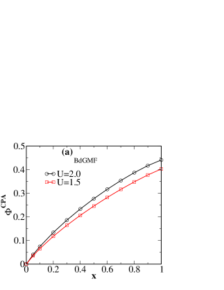
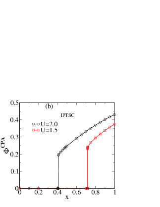
Figure 4: The disorder-averaged superconducting order parameter, $\Phi^{CPA}$, as a function of disorder, $x$ computed within BdGMF (upper panel) and IPTSC (lower panel).

5 Conclusions

In this paper, a disordered attractive Hubbard model with spatially random interaction sites is investigated by combining DMFT, CPA and IPTSC as an impurity solver at half filling. We have computed local quantities such as diagonal and off diagonal spectral function for different values of U and $x$. By using local off diagonal spectral functions, we have computed superconducting order parameter. We find a doping (disorder) induced metal to superconductor transition. The transition is first order for low interaction strengths, but becomes continuous for $U>U_{c}$. The critical disorder needed to achieve superconductivity becomes nearly zero beyond $U>U_{c}$. The experiments on Tl doped PbTe, mentioned in the introduction, show that [3, 4] superconductivity is induced with just 0.3% concentration of Tl. From our figure 3, we would then conclude that the local attraction strength at the Tl-sites is quite larger than the bandwidth. To highlight the effects of dynamical fluctuations beyond static mean-field, we have calculated the superconducting order parameter in IPTSC and BdGMF frameworks. In parallel to the IPTSC scenario described above, the BdGMF approach shows a metal to superconductor transition, however the transition is always continuous for all attractive interaction strengths.

Authors thank CSIR, India and JNCASR, India for funding the research.

References

- [1] P. A. Lee and T. V. Ramakrishnan: Rev. Mod. Phys. 57 (1985) 287.
- [2] D. Belitz and T. R. Kirkpatrick: Rev. Mod. Phys. 66 (1994) 261.
- [3] Y. Matsushita, H. Bluhm, T. H. Geballe, and I. R. Fisher: Phys. Rev. Lett. 94 (2005) 157002.
- [4] Y. Matsushita, P. A. Wianecki, A. T. Sommer, T. H. Geballe, and I. R. Fisher: Phys. Rev. B 74 (2006) 134512.
- [5] R. Micnas, J. Ranninger, and S. Robaszkiewicz: Rev. Mod. Phys. 62 (1990) 113.
- [6] A. Georges, G. Kotliar, W. Krauth, and M. Rozenberg J: Rev. Mod. Phys. 68 (1996) 13.
- [7] G. Kotliar and D. Vollhardt: Physics Today 57 (2004) 53-59.
- [8] D. Vollhardt: AIP Conference Proceedings 1297 (2010) 339.
- [9] R. J. Elliott, J. A. Krumhansl, and P. L. Leath: Rev. Mod. Phys. 46 (1974) 465.
- [10] V. Janis and D. Vollhardt : Phys. Rev. B 46 (1992) 15712.
- [11] A. Garg, H. R. Krishnamurthy, and M. Randeria: Phys. Rev. B 72 (2005) 024517.
- [12] V. B. Shenoy: Phys. Rev. B 78 (2008) 134503.
- [13] G. Litak and B. L. Gyrffy: Phys. Rev. B 62 (1999) 6629.
- [14] Naushad Ahmad Kamar and N. S. Vidhyadhiraja: J. Phys. Condens. Matter (2014) 26 095701.
- [15] Naushad Ahmad Kamar and N. S. Vidhyadhiraja: arXiv:1403.1972 (2014).
- [16] J. Bauer, A. C. Hewson, and N. Dupuis: Phys. Rev. B 79 (2009) 214518.
- [17] Akihisa Koga and Philipp Werner: Phys. Rev. A 84 (2011) 023638.
- [18] Naushad Ahmad Kamar: M. S.(Engg.) Thesis, Theoretical Sciences Unit, JNCASR, Bangalore, India (2013).
- [19] Thomas Maier et. al : Rev. Mod. Phys. 77 (2005) 1027.